Denoising IMU Gyroscopes with Deep Learning for Open-Loop Attitude Estimation

Abstract

This paper proposes a learning method for denoising gyroscopes of Inertial Measurement Units (IMUs) using ground truth data, and estimating in real time the orientation (attitude) of a robot in dead reckoning. The obtained algorithm outperforms the state-of-the-art on the (unseen) test sequences. The obtained performances are achieved thanks to a well-chosen model, a proper loss function for orientation increments, and through the identification of key points when training with high-frequency inertial data. Our approach builds upon a neural network based on dilated convolutions, without requiring any recurrent neural network. We demonstrate how efficient our strategy is for 3D attitude estimation on the EuRoC and TUM-VI datasets. Interestingly, we observe our dead reckoning algorithm manages to beat top-ranked visual-inertial odometry systems in terms of attitude estimation although it does not use vision sensors. We believe this paper offers new perspectives for visual-inertial localization and constitutes a step toward more efficient learning methods involving IMUs. Our open-source implementation is available at https://github.com/mbrossar/denoise-imu-gyro.

I Introduction

IInertial Measurement Units (IMUs) consist of gyroscopes that measure angular velocities, i.e. the rate of change of the sensor’s orientation, and accelerometers that measure proper accelerations [1]. IMUs allow estimating a robot’s trajectory relative to its starting position, a task called odometry [2].

Small and cheap IMUs are ubiquitous in smartphones, industrial and robotics applications, but suffer from difficulties to estimate sources of error, such as axis-misalignment, scale factors and time-varying offsets [3, 4]. Hence, IMU signals are not only noisy, but they are biased. In the present paper, we propose to leverage deep learning for denoising the gyroscopes (gyros) of an IMU, that is, reduce noise and biases. As a byproduct, we obtain accurate attitude (i.e. orientation) estimates simply by open-loop integration of the obtained noise-free gyro measurements.

I-A Links and Differences with Existing Literature

IMUs are generally coupled with complementary sensors to obtain robust pose estimates in sensor-fusion systems [5], where the supplementary information is provided by either cameras in Visual-Inertial Odometry (VIO) [6, 7, 8], LiDAR, GNSS, or may step from side information about the model [9, 10, 11, 12]. To obtain accurate pose estimates, a proper IMU calibration is required, see e.g. the widely used Kalibr library [13, 3], which computes offline the underlying IMU intrinsic calibration parameters, and extrinsic parameters between the camera and IMU. Our approach, which is recapped in Figure 1, is applicable to any system equipped with an IMU. It estimates offline the IMU calibration parameters and extends methods such as [13, 3] to time-varying signal corrections.

Machine learning (more specifically deep learning) has been recently leveraged to perform LiDAR, visual-inertial, and purely inertial localization, where methods are divided into supervised [14, 15, 16, 17] and unsupervised [18]. Most works extract relevant features in the sensors’ signals which are propagated in time through recurrent neural networks, whereas [19] proposes convolutional neural networks for pedestrian inertial navigation. A related approach [20] applies reinforcement learning for guiding the user to properly calibrate visual-inertial rigs. Our method is supervised (we require ground truth poses for training), leverages convolutions rather than recurrent architectures, and outperforms the latter approach. We obtain excellent results while requiring considerably fewer data and less time. Finally, the reference [17] estimates orientation with an IMU and recurrent neural networks, but our approach proves simpler.

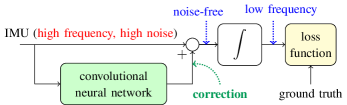
Figure 1: Schematic illustration of the proposed method. The convolutional neural network computes gyro corrections (based on past IMU measurements) that filter undesirable errors in the raw IMU signals. We then perform open-loop time integration on the noise-free measurements for regressing low frequency errors between ground truth and estimated orientation increments.

I-B Contributions

Our main contributions are as follows:

• detailed modelling of the problem of learning orientation increments from low-cost IMUs;

• the convolutional neural network which regresses gyro corrections and whose features are carefully selected;

• the training procedure which involves a trackable loss function for estimating relative orientation increments;

• the approach evaluation on datasets acquired by a drone and a hand-held device [21, 22], where our method outperforms [17] and competes with VIO methods [6, 7] although it does not use vision;

• perspectives towards more efficient VIO and IMU based learning methods;

• a publicly available open-sourced code, where training is done in 5 minutes per dataset.

II Kinematic & Low-Cost IMU Models

We detail in this section our model.

II-A Kinematic Model based on Orientation Increments

The 3D orientation of a rigid platform is obtained by integrating orientation increments, that is, gyro outputs of an IMU, through

$$\mathbf{R}_{n}=\mathbf{R}_{n-1}\exp\left(\bm{\omega}_{n}dt\right),$$ (1)

where the rotation matrix $\mathbf{R}_{n}\in SO(3)$ at timestamp $n$ maps the IMU frame to the global frame, the angular velocity $\bm{\omega}_{n}\in\mathbb{R}^{3}$ is averaged during $dt$, and with $\exp(\cdot)$ the $SO(3)$ exponential map. The model (1) successively integrates in open-loop $\bm{\omega}_{n}$ and propagates estimation errors. Indeed, let $\hat{\mathbf{R}}_{n}$ denotes an estimate of $\mathbf{R}_{n}$. The error present in $\hat{\mathbf{R}}_{n-1}$ is propagated in $\hat{\mathbf{R}}_{n}$ through (1).

II-B Low-Cost Inertial Measurement Unit (IMU) Sensor Model

The IMU provides noisy and biased measurements of angular rate $\bm{\omega}_{n}$ and specific acceleration $\mathbf{a}_{n}$ at high frequency ($200\text{\,}\mathrm{H}\mathrm{z}$ in our experiments) as, see [4, 3],

$$\mathbf{u}_{n}^{\mathrm{\textsc{imu}}}=\begin{bmatrix}\bm{\omega}_{n}^{\mathrm{\textsc{imu}}}\\ \mathbf{a}_{n}^{\mathrm{\textsc{imu}}}\end{bmatrix} =\mathbf{C}\begin{bmatrix}\bm{\omega}_{n}\\ \mathbf{a}_{n}\end{bmatrix}+\mathbf{b}_{n}+\bm{\eta}_{n},$$ (2)

where $\mathbf{b}_{n}\in\mathbb{R}^{6}$ are quasi-constant biases, $\bm{\eta}_{n}\in\mathbb{R}^{6}$ are commonly assumed zero-mean white Gaussian noises, and

$$\mathbf{a}_{n}=\mathbf{R}_{n-1}^{T}\left(\left(\mathbf{v}_{n}-\mathbf{v}_{n-1}\right)/dt-\mathbf{g}\right)\in\mathbb{R}^{3}$$ (3)

is the acceleration in the IMU frame without the effects of gravity $\mathbf{g}$, with $\mathbf{v}_{n}\in\mathbb{R}^{3}$ the IMU velocity expressed in the global frame. The intrinsic calibration matrix

$$\mathbf{C}=\begin{bmatrix}\mathbf{S}_{\bm{\omega}}\mathbf{M}_{\bm{\omega}}&\mathbf{A}\\ \mathbf{0}_{3\times 3}&\mathbf{S}_{\mathbf{a}}\mathbf{M}_{\mathbf{a}}\end{bmatrix}\approx\mathbf{I}_{6}$$ (4)

contains the information for correcting signals: axis misalignments (matrices $\mathbf{M}_{\bm{\omega}}\approx\mathbf{I}_{3}$ and $\mathbf{M}_{\mathbf{a}}\approx\mathbf{I}_{3}$); scale factors (diagonal matrices $\mathbf{S}_{\bm{\omega}}\approx\mathbf{I}_{3}$ and $\mathbf{S}_{\mathbf{a}}\approx\mathbf{I}_{3}$); and linear accelerations on gyro measurements, a.k.a. g-sensitivity (matrix $\mathbf{A}\approx\mathbf{0}_{3\times 3}$). Remaining intrinsic parameters, e.g. level-arm between gyro and accelerometer, can be found in [4, 3].

We now make three remarks regarding (1)-(4):

1. equations (2)-(4) represent a model that approximates reality. Indeed, calibration parameters $\mathbf{C}$ and biases $\mathbf{b}_{n}$ should both depend on time as they vary with temperature and stress [1, 4], but are difficult to estimate in real-time. Then, vibrations and platform excitations due to, e.g. rotors, make Gaussian noise $\bm{\eta}_{n}$ colored in practice [23], albeit commonly assumed white;

2. substituting actual measurements $\bm{\omega}_{n}^{\mathrm{\textsc{imu}}}$ in place of true value $\bm{\omega}_{n}$ in (1) leads generally to quick drift (in a few seconds) and poor orientation estimates;

3. in terms of method evaluation, one should always compare the learning method with respect to results obtained with a properly calibrated IMU as a proper estimation of the parameters $\mathbf{C}$ and $\mathbf{b}_{n}$ in (2) actually leads to surprisingly precise results, see Section IV.

III Learning Method for Denoising the IMU

We describe in this section our approach for regression of noise-free gyro increments $\hat{\bm{\omega}}_{n}$ in (2) in order to obtain accurate orientation estimates by integration of $\hat{\bm{\omega}}_{n}$ in (1). Our goal thus boils down to estimating $\mathbf{b}_{n}$, $\bm{\eta}_{n}$, and correcting the misknown $\mathbf{C}$.

III-A Proposed Gyro Correction Model

Leveraging the analysis of Section II, we compute the noise-free increments as

$$\hat{\bm{\omega}}_{n}=\hat{\mathbf{C}}_{\bm{\omega}}\bm{\omega}_{n}^{\mathrm{\textsc{imu}}}+\tilde{\bm{\omega}}_{n},$$ (5)

with $\hat{\mathbf{C}}_{\bm{\omega}}=\hat{\mathbf{S}}_{\bm{\omega}}\hat{\mathbf{M}}_{\bm{\omega}}\in\mathbb{R}^{3\times 3}$ the intrinsic parameters that account for gyro axis-misalignment and scale factors, and where the gyro bias is included in the gyro correction $\tilde{\bm{\omega}}_{n}=\hat{\mathbf{c}}_{n}+\hat{\mathbf{b}}$, where $\hat{\mathbf{c}}_{n}$ is time-varying and $\hat{\mathbf{b}}$ is the static bias. Explicitly considering the small accelerometer influence $\mathbf{A}$, see (2)-(4), does not affect the results so it is ignored.

CNN layer #	1	2	3	4	5
kernel dim.	7	7	7	7	1
dilatation gap	1	4	16	64	1
channel dim.	16	32	64	128	1

Figure 2: Proposed neural network structure which computes gyro correction $\tilde{\bm{\omega}}_{n}$ in (5) from the $N$ past IMU measurements. We set the Convolutional Neural Networks (CNNs) as indicated in the table, and define between two convolutional layers a batchnorm layer [24] and a smooth GELU activation function [25] (magenta arrows). The adopted structure defines the window size $N=\max\left(\text{kernel dim.}\times\text{dilation gap}\right)=7\times 64=448$, corresponding to $2.24\text{\,}\mathrm{s}$ of past information, and has been found after trial-and-error on datasets [21, 22].

We now search to compute $\tilde{\bm{\omega}}_{n}$ and $\hat{\mathbf{C}}_{\bm{\omega}}$. The neural network described in Section III-B computes $\tilde{\bm{\omega}}_{n}$ by leveraging information present in a past local window of size $N$ around $\bm{\omega}_{n}^{\mathrm{\textsc{imu}}}$. In contrast, we let $\hat{\mathbf{C}}_{\bm{\omega}}$ be static parameters initialized at $\mathbf{I}_{3}$ and optimized during training since each considered dataset uses one IMU. The learning problem involving a time varying $\hat{\mathbf{C}}_{\bm{\omega}}$ and/or multiple IMUs is let for future works.

The consequences of opting for the model (5) and the proposed network structure are as follows. First, the corrected gyro is initialized on the original gyro $\hat{\bm{\omega}}_{n}\approx\bm{\omega}_{n}^{\mathrm{\textsc{imu}}}$, with $\hat{\mathbf{C}}_{\bm{\omega}}=\mathbf{I}_{3}$ and $\tilde{\bm{\omega}}_{n}\approx\mathbf{0}_{3}$ before training. This way, the method improves the estimates as soon as the first training epoch. Then, our method is intrinsically robust to overfitting as measurements outside the local window, i.e. whose timestamps are less than $n-N$ or greater than $n$, see Figure 2, do not participate in infering $\tilde{\bm{\omega}}_{n}$. This allows to train the method with 8 or less minutes of data, see Section IV-A.

III-B Dilated Convolutional Neural Network Structure

We define here the neural network structure which infers the gyro correction as

$$\tilde{\bm{\omega}}_{n}=f(\mathbf{u}_{n-N}^{\mathrm{\textsc{imu}}},\ldots,\mathbf{u}_{n}^{\mathrm{\textsc{imu}}}),$$ (6)

where $f(\cdot)$ is the function defined by the neural network. The network should extract information at temporal multi-scales and compute smooth corrections. Note that, the input of the network consists of IMU data, that is, gyros naturally, but also accelerometers signals. Indeed, from (3), if the velocity varies slowly between successive increments we have

$$\mathbf{a}_{n+1}-\mathbf{a}_{n} \approx-(\mathbf{R}_{n}-\mathbf{R}_{n-1})^{T}\mathbf{g}$$

$$\approx-(\exp\left(-\bm{\omega}_{n}dt\right)-\mathbf{I}_{3})\mathbf{R}_{n-1}^{T}\mathbf{g},$$ (7)

which also provides information about angular velocity. This illustrates how $\mathbf{a}_{n}$ can be used, albeit the neural network does not assume small velocity variation.

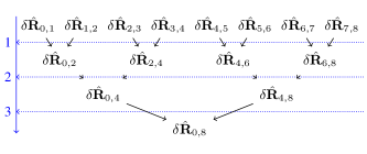
Figure 3: Time efficient computation of the loss (9) by viewing the orientation integration (8) as a tree of matrix multiplications. Computation for length $j$ requires $\log_{2}(j)$ “batch” operations as denoted by the blue vertical arrow on the left. We see we need 3 batches of parallel operations for $j=8$ on the chart above. In the same way, we only need 5 operations for $j=32$.

We leverage dilated convolutions that infer a correction based on a local window of $N=448$ previous measurements, which represents $2.24\text{\,}\mathrm{s}$ of information before timestamp $n$ in our experiments. Dilated convolutions are a method based on convolutions applied to input with defined dilatation gap, see [26], which: $i$) supports exponential expansion of the receptive field, i.e., $N$, without loss of resolution or coverage; $ii$) is computationally efficient with few memory consumption; and $iii$) maintains the temporal ordering of data. We thus expect the network to detect and correct various features such as rotor vibrations that are not modeled in (2). Our configuration given in Figure 2 requires learning $77\,052$ parameters, which is extremely low and contrasts with recent (visual-)inertial learning methods, see e.g. [18] Figure 2, where IMU processing only requires more than $2\,600\,000$ parameters.

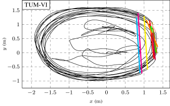
Figure 4: Horizontal ground truth trajectory for the sequence room 1 of [22]. Ground truth is periodically absent due to occlusions of the hand-held device from the motion capture system, see the color lines on the right of the figure.

III-C Loss Function based on Integrated Gyro Increments

Defining a loss function directly based on errors $\bm{\omega}_{n}-\hat{\bm{\omega}}_{n}$ requires having a ground truth $\bm{\omega}_{n}$ at IMU frequency ($200\text{\,}\mathrm{H}\mathrm{z}$), which is not feasible in practice as the best tracking systems are accurate at $20$-$120\text{\,}\mathrm{H}\mathrm{z}$. In place, we suggest defining a loss based on the following integrated increments

$$\delta\mathbf{R}_{i,i+j} =\mathbf{R}_{i}^{T}\mathbf{R}_{i+j}=\prod_{k=i}^{i+j-1}\exp\left(\bm{\omega}_{k}\right),$$ (8)

i.e., where the IMU frequency is reduced by a factor $j$. We then compute the loss for a given $j$ as

$$\mathcal{L}_{j} =\sum_{i}\rho\left(\log\left(\delta\mathbf{R}_{i,i+j}\delta\hat{\mathbf{R}}_{i,i+j}^{T}\right)\right),$$ (9)

where $\log(\cdot)$ is the $SO(3)$ logarithm map, and $\rho(\cdot)$ is the Huber loss function. We set in our experiments the Huber loss parameter to 0.005, and define our loss function as

$$\mathcal{L}=\mathcal{L}_{16}+\mathcal{L}_{32}.$$ (10)

The motivations for (9)-(10) are as follows:

• the choice of Huber loss $\rho(\cdot)$ yields robustness to ground truth outliers;

• (8) is invariant to rotations which suits well IMUs, whose gyro and accelerometer measurements are respectively invariant to rotations and yaw changes [2, 27], i.e., left shifting $\mathbf{R}_{n}\leftarrow\delta\mathbf{R}\mathbf{R}_{n}$ and $\hat{\mathbf{R}}_{n}\leftarrow\delta\mathbf{R}\hat{\mathbf{R}}_{n}$ with $\delta\mathbf{R}_{n}\in SO(3)$ leaves (9) unchanged;

• the choice of (10) corresponds to error increments at $200/16\approx$12\text{\,}\mathrm{H}\mathrm{z}$$ and $200/32\approx$6\text{\,}\mathrm{H}\mathrm{z}$$, which is barely slower than ground truth. Setting too high a $j$, or in the extreme case using a loss based on the overall orientation error $\mathbf{R}_{n}^{T}\hat{\mathbf{R}}_{n}$, would make the algorithm prone to overfitting, and hence makes the method too sensitive to specific trajectory patterns of training data.

dataset	sequence	VINS-	VINS-Mono	Open-	Open-VINS	zero	raw	OriNet	calibrated IMU	proposed
		Mono [7]	(loop-closure)	VINS [6]	(proposed)	motion	IMU	[17]	(proposed)	IMU
	MH 02 easy	1.34/1.32	0.57/0.50	1.11/1.05	1.21/1.12	44.4/43.7	146/130	5.75/0.51	7.09/1.49	1.39/0.85
	MH 04 difficult	1.44/1.40	1.06/1.00	1.60/1.16	1.40/0.89	42.3/41.9	130/77.9	8.85/7.27	5.64/2.53	1.40/0.25
EuRoC	V1 01 easy	0.97/0.90	0.57/0.44	0.80/0.67	0.80/0.67	114/76	71.3/71.2	6.36/2.09	6.65/3.95	1.13/0.49
[21]	V1 03 difficult	4.72/4.68	4.06/4.00	2.32/2.27	2.25/2.20	81.4/80.5	119/84.9	14.7/11.5	3.56/2.04	2.70/0.96
	V2 02 medium	2.58/2.41	1.83/1.61	1.85/1.61	1.81/1.57	93.9/93.5	117/86	11.7/6.03	4.63/2.30	3.85/2.25
	average	2.21/2.14	1.62/1.52	1.55/1.37	1.50/1.30	66.1/66.1	125/89.0	9.46/5.48	5.51/2.46	2.10/0.96
	room 2	0.60/0.45	0.69/0.50	2.47/2.36	1.95/1.84	91.8/90.4	118/88.1	–/–	10.6/10.5	1.31/1.18
TUM-VI	room 4	0.76/0.63	0.66/0.51	0.97/0.88	0.93/0.83	107/103	74.1/48.2	–/–	2.43/2.30	1.48/0.85
[22]	room 6	0.58/0.38	0.54/0.33	0.63/0.51	0.60/0.51	138/131	94.0/76.1	–/–	4.39/4.31	1.04/0.57
	average	0.66/0.49	0.63/0.45	1.33/1.25	1.12/1.05	112/108	95.7/70.8	–/–	5.82/5.72	1.28/0.82

Table 1: Absolute Orientation Error (AOE) in terms of 3D orientation/yaw, in degree, on the test sequences. We see our approach competes with VIO (while entirely based on IMU signals) and outperforms other inertial methods. Results from OriNet are unavailable on the TUM-VI dataset.

III-D Efficient Computation of (8)-(10)

First, note that thanks to parallelization applying e.g. $\exp(\cdot)$, to one or parallelly to many $\hat{\bm{\omega}}_{n}$ takes similar execution time on a GPU (we found experimentally that one operation takes $5\text{\,}\mathrm{m}\mathrm{s}$ whereas 10 million operations in parallel takes $70\text{\,}\mathrm{m}\mathrm{s}$, that is, the time per operation drops to $7\text{\,}\mathrm{n}\mathrm{s}$). We call an operation that is parallelly applied to many instances a batch operation. That said, an apparent drawback of (8) is to require $j$ matrix multiplications, i.e. $j$ operations. However, first, we may compute ground truth $\delta\mathbf{R}_{i,i+j}$ only once, store it, and then we only need to compute $\delta\hat{\mathbf{R}}_{i,i+j}$ multiple times. Second, by viewing (8) as a tree of matrix multiplications, see Figure 3, we reduce the computation to $\log_{2}(j)$ batch GPU operations only. We finally apply sub-sampling and take one $i$ every $j$ timestamps to avoid counting multiple times the same increment. Training speed is thus increased by a factor $32/\log_{2}(32)\approx 6$.

III-E Training with Data Augmentation

Data augmentation is a way to significantly increase the diversity of data available for training without actually collecting new data, to avoid overfitting. This may be done for the IMU model of Section II by adding Gaussian noise $\bm{\eta}_{n}$, adding static bias $\mathbf{b}_{n}$, uncalibrating the IMU, and shifting the orientation of the IMU in the accelerometer measurement. The two first points were noted in [17], whereas the two latter are to the best of our knowledge novel.

Although each point may increase the diversity of data, we found they do not necessarily improve the results. We opted for addition of a Gaussian noise (only), during each training epoch, whose standard deviation is the half the standard deviation that the dataset provides ($0.01\text{\,}\mathrm{d}\mathrm{e}\mathrm{g}\mathrm{/}\mathrm{s}$).

IV Experiments

We evaluate the method in terms of 3D orientation and yaw estimates, as the latter are more critical regarding long-term odometry estimation [28, 2].

IV-A Dataset Descriptions

We divide data into training, validation, and test sets, defined as follows, see Chapter I.5.3 of [29]. We optimize the neural network and calibration parameters on the training set. Validation set intervenes when training is over, and provides a biased evaluation, as the validation set is used for training (data are seen, although never used for “learning”). The test set is the gold standard to provide an unbiased evaluation. It is only used once training (using the training and validation sets) is terminated. The datasets we use are as follows.

IV-A1 EuRoC

the dataset [21] contains image and inertial data at $200\text{\,}\mathrm{H}\mathrm{z}$ from a micro aerial vehicle divided into 11 flight trajectories of 2-3 minutes in two environments. The ADIS16448 IMU is uncalibrated and we note ground truth from laser tracker and motion capture system is accurately time-synchronized with the IMU, although dynamic motions deteriorate the measurement accuracy. As yet noticed in [6], ground truth for the sequence V1 01 easy needs to be recomputed. The sequences MH and V1 were acquired in two consecutive days, and the sequences V2 more than three months latter. Thus the network should adapt to varying bias.

We define the train set as the first $50\text{\,}\mathrm{s}$ of the six sequences MH{01,03,05}, V1{02}, V2{01,03}, the validation set as the remaining ending parts of these sequences, and we constitute the test set as the five remaining sequences. We show in Section IV-E that using only 8 minutes of accurate data for training - the beginning and end of each trajectory are the most accurately measured - is sufficient to obtain relevant results.

IV-A2 TUM-VI

the recent dataset [22] consists of visual-inertial sequences in different scenes from an hand-held device. The cheap BMI160 IMU logs data at $200\text{\,}\mathrm{H}\mathrm{z}$ and was properly calibrated. Ground truth is accurately time-synchronized with the IMU, although each sequence contains periodic instants of duration $0.2\text{\,}\mathrm{s}$ where ground truth is unavailable as the acquisition platform was hidden from the motion capture system, see Figure 4. We take the 6 room sequences, which are the sequences having longest ground truth (2-3 minutes each).

We define the train set as the first $50\text{\,}\mathrm{s}$ of the sequences room 1, room 3, and room 5, the validation set as the remaining ending parts of these sequences, and we set the test set as the 3 other room sequences. This slipt corresponds to $45\,000$ training data points ($90\,000$ for EuRoC) which is in the same order as the number of optimized parameters, $77\,052$, and requires regularization techniques such as weight decay and dropout during training.

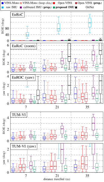
Fig. 5: Relative Orientation Error (ROE) in terms of 3D orientation and yaw errors on the test sequences. Our method outperforms calibrated IMU and competes with VIO methods albeit based only on IMU signals. Raw IMU is way off and results from OriNet on TUM-VI are unavailable.

IV-B Method Implementation & Training

Our open-source method is implemented based on PyTorch 1.5, where we configure the training hyperparameters as follows. We set weight decay with parameter 0.1, and dropout with 0.1 the probability of an element to be set equal to zero. Both techniques reduce overfitting.

We choose the ADAM optimizer [30] with cosines warning restart scheduler [31] where learning rate is initialized at 0.01. We train for $1800$ epochs, which is is very fast as it takes less than 5 minutes for each dataset with a GTX 1080 GPU device.

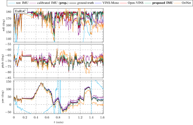
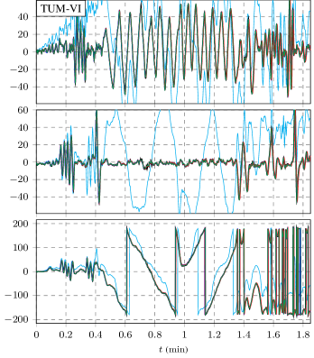
Fig. 6: Orientation estimates on the test sequence MH 04 difficult of [21] (left), and room 4 of [22] (right). Our method removes errors of the calibrated IMU and competes with VIO algorithms.

IV-C Compared Methods

We compare a set of methods based on camera and/or IMU.

IV-C1 Methods Based on the IMU Only

we compare the following approaches:

• raw IMU, that is an uncalibrated IMU. It refers also to the proposed method once initialized but not trained;

• OriNet [17], which is based on recurrent neural networks, and whose training and test sets correspond to ours;

• calibrated IMU, that is, our method where the 12 parameters $\hat{\mathbf{C}}_{\bm{\omega}}$ and $\tilde{\bm{\omega}}_{n}$ are constant, nonzero, and optimized. This can be seen by enforcing to zero the network inputs, i.e. setting the IMU gyros and accelerometers in (6) as $\mathbf{u}_{n}=\mathbf{0}_{6}$, both during training and evaluation;

• proposed IMU, which is our learning based method described in Section III.

IV-C2 Methods Based on Camera and the IMU

we run each of the following method with the same setting, ten times to then average results, and on a Dell Precision Tower 7910 workstation desktop, i.e., without deterioration due to computational limitations [28]. We compare:

• VINS-Mono [7], a monocular VIO framework with notable performances on the EuRoC benchmark [28];

• VINS-Mono (loop closure), which is the original VINS-Mono [7] reinforced with loop-closure ability;

• Open-VINS [6], a versatile filter-based visual-inertial estimator for which we choose the stereo configuration, and that is top-ranked on the drone dataset of [32];

• Open-VINS (proposed), which is Open-VINS of [6] but where gyro inputs are the proposed corrected gyro measurements (5) outputted by our method (trained on sequences that are of course different from those used for evaluation).

IV-D Evaluation Metrics

We evaluate the above methods using the following metrics that we compute with the toolbox of [6].

IV-D1 Absolute Orientation Error (AOE)

which computes the mean square error between the ground truth and estimates for a given sequence as

$$\mathrm{AOE}=\sqrt{\sum_{n=1}^{M}\frac{1}{M}\|\log\left(\mathbf{R}_{n}^{T}\hat{\mathbf{R}}_{n}\right)\|_{2}^{2}},$$ (11)

with $M$ the sequence length, $\log(\cdot)$ the $SO(3)$ logarithm map, and where the estimated trajectory has been aligned on the ground truth at the first instant $n=0$.

IV-D2 Relative Orientation Error (ROE)

which is computed as [27]

$$\mathrm{ROE}=\|\log\left(\delta\mathbf{R}_{n,g(n)}^{T}\delta\hat{\mathbf{R}}_{n,g(n)}\right)\|_{2},$$ (12)

for each pair of timestamps $\left(n,g(n)\right)$ representing an IMU displacement of 7, 21 or 35 meters. Collecting the error (12) for all the pairs of sub-trajectories generates a collection of errors where informative statistics such as the median and percentiles are calculated. As [27, 28, 6], we strongly recommend ROE for comparing odometry estimation methods since AOE is highly sensitive to the time when the estimation error occurs. We finally consider slight variants of (11)-(12) when considering yaw (only) errors, and note that errors of visual methods generally scale with distance travelled whereas errors of inertial only methods scales with time. We provide in the present paper errors w.r.t. distance travelled to favor comparison with benchmarks such as [28], and same conclusions hold when computing ROE as function of different times.

IV-E Results

Results are given in term of AOE and ROE respectively in Table 1 and Figure 5. Figure 6 illustrates roll, pitch and yaw estimates for a test sequence of each dataset, and Figure 7 shows orientation errors. We note that:

IV-E1 Uncalibrated IMU is Unreliable

raw IMU estimates deviate from ground truth in less than $10\text{\,}\mathrm{s}$, see Figure 6.

IV-E2 Calibrated IMU Outperforms OriNet

only calibrating an IMU (via our optimization method) leads to surprisingly accurate results, see e.g., Figure 6 (right) where it is difficult to distinguish it from ground truth. This evidences cheap sensors can provide very accurate information once they are correctly calibrated.

IV-E3 The Proposed Method Outperforms Inertial Methods

OriNet [17] is outperformed. Moreover, our method improves accurate calibrated IMU by a factor 2 to 4. Our approach notably obtains as low as a median error of $1.34\text{\,}\deg\mathrm{/}\mathrm{m}\mathrm{i}\mathrm{n}$ and $0.68\text{\,}\deg\mathrm{/}\mathrm{m}\mathrm{i}\mathrm{n}$ on respectively EuRoC and TUM-VI datasets.

IV-E4 The Proposed Method Competes with VIO

our IMU only method is accurate even on the high motion dynamics present in both datasets, see Figure 6, and competes with VINS-Mono and Open-VINS, although trained with only a few minutes of data.

Finally, as the performance of each method depends on the dataset and the algorithm setting, see Figure 5, it is difficult to conclude which VIO algorithm is the best.

IV-F Further Results and Comments

We provide a few more comments, supported by further experimental results.

IV-F1 Small Corrections Might Lead to Large Improvement

the calibrated and corrected gyro signals are visually undistinguishable: differences between them rely in corrections $\tilde{\bm{\omega}}_{n}$ of few $\mathrm{d}\mathrm{e}\mathrm{g}\mathrm{/}\mathrm{s}$, as shown in Figure 8. However, they bring drastic improvement in the estimates. This confirms the interest of leveraging neural networks for model correction (2)-(4).

IV-F2 The Proposed Method is Well Suited to Yaw Estimation

according to Table 1 and Figure 5, we see yaw estimates are particularly accurate. Indeed, VIO methods are able to recover at any time roll and pitch thanks to accelerometers, but the yaw estimates drift with time. In contrast our dead-reckoning method never has access to information allowing to recover roll and pitch during testing, and nor does it use “future” information such as VINS-Mono with loop-closure ability. We finally note that accurate yaw estimates could be fruitful for yaw-independent VIO methods such as [8].

IV-F3 Correcting Gyro Slightly Improves Open-VINS [6]

both methods based on Open-VINS perform similarly, which is not surprising as camera alone already provides accurate orientation estimates and the gyro assists stereo cameras.

IV-F4 Our Method Requires few Computational Ressources

each VIO method performs here at its best while resorting to high computational requirements, and we expect our method - once trained - is very attractive when running onboard with limited resources. Note that, the proposed method performs e.g. 3 times better in terms of yaw estimates than a slightly restricted VINS-Mono, see Figure 3 of [28].

V Discussion

We now provide the community with feedback regarding the method and its implementation. Notably, we emphasize a few points that seem key to a successful implementation when working with a low-cost high frequency IMU.

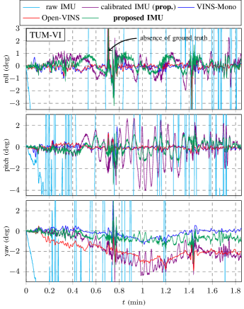
Fig. 7: Orientation errors on the sequence room 4 of [22]. Our method removes errors of the calibrated IMU and competes with VIO algorithms.

V-A Key Points Regarding the Dataset

One should be careful regarding the quality of data, especially when IMU is sampled at high-frequency. This concerns:

V-A1 IMU Signal

the IMU signal acquisition should be correct with constant sampling time.

V-A2 Ground Truth Pose Accuracy

we note that the EuRoC ground truth accuracy is better at the beginning of the trajectory. As such, training with only this part of data (the first $50\text{\,}\mathrm{s}$ of the training sequences) is sufficient (and best) to succeed.

V-A3 Ground Truth Time-Alignement

the time alignment between ground truth and IMU is significant for success, otherwise the method is prone to learn a time delay.

We admit that our approach requires a proper dataset, which is what constitutes its main limitation.

V-B Key Points Regarding the Neural Network

Our conclusions about the neural network are as follows.

V-B1 Activation Function

the GELU and other smooth activation functions [25], such as ELU, perform well, whereas ReLU based network is more prone to overfit. We believe ReLU activation function favors sharp corrections which does not make sense when dealing with physical signals.

V-B2 Neural Network Hyperparameters

increasing the depth, channel and/or kernel sizes of the network, see Figure 2, does not systematically lead to better results. We tuned these hyperparameters with random search, although more sophisticated methods such as [33] exist.

V-B3 Normalization Layer

batchnorm layer improves both training speed and accuracy [24], and is highly recommended.

V-B4 Accelerometers are Relevant

we test our approach without accelerometer, a.k.a. ablation study experiment, where the neural network obtains 50 % more errors than proposed IMU in term of ROE. It indicates how accelerometer are useful, see an instinctive reason in Section III-B.

V-B5 Reccurent Neural Network obtains Higher Errors

we also compare our same approach where LSTM replaces the dilated convolutions in the network structure. This type of neural network obtains around 40 % more errors than proposed IMU in term of ROE, while requiring also more time to be trained.

V-C Key Points Regarding Training

As in any machine learning application, the neural network architecture is a key component among others [29]. Our comments regarding training are as follows:

V-C1 Optimizer

the ADAM optimizer [30] performs well.

V-C2 Learning Rate Scheduler

adopting a learning rate policy with cosinus warning restart [31] leads to substantial improvement and helps to find a correct learning rate.

V-C3 Regularization

dropout and weight decay hyperparameters are crucial to avoid overfitting. Each has a range of ideal values which is quickly tuned with basic grid-search.

Fig. 8: Gyro correction $\tilde{\bm{\omega}}_{n}$ on the sequence room 4 of [22]. We see we manage to divide orientation errors by a factor at least 2 w.r.t. calibrated IMU applying corrections whose amplitude is as low as $1\text{\,}\mathrm{d}\mathrm{e}\mathrm{g}\mathrm{/}\mathrm{s}$ (max).

V-D Remaining Key Points

We finally outline two points that we consider useful to the practitioner:

V-D1 Orientation Implementation

we did not find any difference between rotation matrix or quaternion loss function implementation once numerical issues are solved, e.g., by enforcing quaternion unit norm. Both implementations result in similar accuracy performance and execution time.

V-D2 Generalization and Transfert Learning

it may prove useful to assess to what extent a learning method is generalizable. The extension of the method, trained on one dataset, to another device or to the same device on another platform is considered as challenging, though, and left for future work.

VI Conclusion

This paper proposes a deep-learning method for denoising IMU gyroscopes and obtains remarkable accurate attitude estimates with only a low-cost IMU, that outperforms state-of-the-art [17]. The core of the approach is based on a careful design and feature selection of a dilated convolutional network, and an appropriate loss function leveraged for training on orientation increment at the ground truth frequency. This leads to a method robust to overfitting, efficient and fast to train, which serves as offline IMU calibration and may enhance it. As a remarkable byproduct, the method competes with state-of-the-art visual-inertial methods in term of attitude estimates on a drone and hand-held device datasets, where we simply integrate noise-free gyro measurements.

We believe the present paper offers new perspectives for (visual-)inertial learning methods. Future work will address new challenges in three directions: learning from multiple IMUs (the current method is reserved for one IMU only which serves for training and testing); learning from moderately accurate ground truth that can be output of visual-inertial localization systems; and denoising accelerometers based on relative increments from preintegration theory [5, 34].

References

- [1] M. Kok, J. D. Hol, and T. B. Schön, “Using Inertial Sensors for Position and Orientation Estimation,” Foundations and Trends® in Signal Processing, vol. 11, no. 1-2, pp. 1–153, 2017.
- [2] D. Scaramuzza and Z. Zhang, “Visual-Inertial Odometry of Aerial Robots,” Encyclopedia of Robotics, 2019.
- [3] J. Rehder, J. Nikolic, T. Schneider, T. Hinzmann, and R. Siegwart, “Extending Kalibr: Calibrating the Extrinsics of Multiple IMUs and of Individual Axes,” in ICRA. IEEE, 2016, pp. 4304–4311.
- [4] J. Rohac, M. Sipos, and J. Simanek, “Calibration of Low-cost Triaxial Inertial Sensors,” IEEE I&M Magazine, vol. 18, no. 6, pp. 32–38, 2015.
- [5] C. Forster, L. Carlone, F. Dellaert, and D. Scaramuzza, “On-Manifold Preintegration for Real-Time Visual-Inertial Odometry,” IEEE T-RO, vol. 33, no. 1, pp. 1–21, 2017.
- [6] P. Geneva, K. Eckenhoff, W. Lee, Y. Yang, and G. Huang, “OpenVINS: A Research Platform for Visual-Inertial Estimation,” in IROS, 2019.
- [7] T. Qin, P. Li, and S. Shen, “VINS-Mono: A Robust and Versatile Monocular Visual-Inertial State Estimator,” IEEE T-RO, vol. 34, no. 4, pp. 1004–1020, 2018.
- [8] J. Svacha, G. Loianno, and V. Kumar, “Inertial Yaw-Independent Velocity and Attitude Estimation for High-Speed Quadrotor Flight,” IEEE RA-L, vol. 4, no. 2, pp. 1109–1116, 2019.
- [9] M. Brossard, A. Barrau, and S. Bonnabel, “RINS-W: Robust Inertial Navigation System on Wheels,” in IROS. IEEE, 2019.
- [10] ——, “AI-IMU Dead-Reckoning,” IEEE T-IV, 2020.
- [11] S. Madgwick, A. Harrison, and R. Vaidyanathan, “Estimation of IMU and MARG Orientation using a Gradient Descent Algorithm,” in ICORR. IEEE, 2011, pp. 1–7.
- [12] A. Solin, S. Cortes, E. Rahtu, and J. Kannala, “Inertial Odometry on Handheld Smartphones,” in FUSION, 2018.
- [13] P. Furgale, J. Rehder, and R. Siegwart, “Unified Temporal and Spatial Calibration for Multi-Sensor Systems,” in IROS. IEEE, 2013, pp. 1280–1286.
- [14] C. Chen, X. Lu, A. Markham, and N. Trigoni, “IONet: Learning to Cure the Curse of Drift in Inertial Odometry,” in AAAI, 2018.
- [15] R. Clark, S. Wang, H. Wen, A. Markham, and N. Trigoni, “VINet: Visual-Inertial Odometry as a Sequence-to-Sequence Learning Problem,” AAAI, 2017.
- [16] H. Yan, Q. Shan, and Y. Furukawa, “RIDI: Robust IMU Double Integration,” in ECCV, 2018.
- [17] M. A. Esfahani, H. Wang, K. Wu, and S. Yuan, “OriNet: Robust 3-D Orientation Estimation With a Single Particular IMU,” IEEE RA-L, vol. 5, no. 2, pp. 399–406, 2020.
- [18] Y. Almalioglu, M. Turan, A. E. Sari, M. R. U. Saputra, P. P. B. de Gusmão, A. Markham, and N. Trigoni, “SelfVIO: Self-Supervised Deep Monocular Visual-Inertial Odometry and Depth Estimation,” arXiv, 2019.
- [19] H. Yan, S. Herath, and Y. Furukawa, “RoNIN: Robust Neural Inertial Navigation in the Wild: Benchmark, Evaluations, and New Methods,” arXiv, 2019.
- [20] F. Nobre and C. Heckman, “Learning to Calibrate: Reinforcement Learning for Guided Calibration of Visual–Inertial Rigs,” IJRR, vol. 38, no. 12-13, pp. 1388–1402, 2019.
- [21] M. Burri, J. Nikolic, P. Gohl, T. Schneider, J. Rehder, S. Omari, M. W. Achtelik, and R. Siegwart, “The EuRoC Micro Aerial Vehicle Datasets,” IJRR, vol. 35, no. 10, pp. 1157–1163, 2016.
- [22] D. Schubert, T. Goll, N. Demmel, V. Usenko, J. Stuckler, and D. Cremers, “The TUM VI Benchmark for Evaluating Visual-Inertial Odometry,” in IROS. IEEE, 2018, pp. 1680–1687.
- [23] G. Lu and F. Zhang, “IMU-Based Attitude Estimation in the Presence of Narrow-Band Noise,” IEEE/ASME Transactions on Mechatronics, vol. 24, no. 2, pp. 841–852, 2019.
- [24] S. Ioffe and C. Szegedy, “Batch Normalization: Accelerating Deep Network Training by Reducing Internal Covariate Shift,” in ICLR, vol. 37, 2015.
- [25] P. Ramachandran, B. Zoph, and Q. V. Le, “Searching for Activation Functions,” ICLR, 2018.
- [26] F. Yu and V. Koltun, “Multi-Scale Context Aggregation by Dilated Convolutions,” ICLR, 2016.
- [27] Z. Zhang and D. Scaramuzza, “A Tutorial on Quantitative Trajectory Evaluation for Visual(-Inertial) Odometry,” in IROS. IEEE, 2018, pp. 7244–7251.
- [28] J. Delmerico and D. Scaramuzza, “A Benchmark Comparison of Monocular Visual-Inertial Odometry Algorithms for Flying Robots,” in ICRA. IEEE, 2018, pp. 2502–2509.
- [29] I. Goodfellow, Y. Bengio, and A. Courville, Deep Learning. The MIT press, 2016.
- [30] D. P. Kingma and J. Ba, “ADAM: A Method for Stochastic Optimization,” in ICLR, 2014.
- [31] I. Loshchilov and F. Hutter, “SGDR: Stochastic Gradient Descent with Warm Restarts,” ICLR, 2016.
- [32] J. Delmerico, T. Cieslewski, H. Rebecq, M. Faessler, and D. Scaramuzza, “Are We Ready for Autonomous Drone Racing? The UZH-FPV Drone Racing Dataset,” in ICRA. IEEE, 2019, pp. 6713–6719.
- [33] L. Li, K. Jamieson, G. DeSalvo, A. Rostamizadeh, and A. Talwalkar, “Hyperband: A Novel Bandit-Based Approach to Hyperparameter Optimization,” JMLR, vol. 18, no. 1, pp. 6765–6816, 2017.
- [34] A. Barrau and S. Bonnabel, “A Mathematical Framework for IMU Error Propagation with Applications to Preintegration,” in ICRA. IEEE, 2020.