A Decomposition Method by Interaction Prediction for the Optimization of Maintenance Scheduling

Abstract

Optimizing maintenance scheduling is a major issue to improve the performance of hydropower plants. We study a system of several physical components of the same family: either a set of turbines, a set of transformers or a set of generators. The components share a common stock of spare parts and experience random failures that occur according to known failure distributions. We seek a deterministic preventive maintenance strategy that minimizes an expected cost depending on maintenance and forced outages of the system. The Auxiliary Problem Principle is used to decompose the original large-scale optimization problem into a sequence of independent subproblems of smaller dimension while ensuring their coordination. Each subproblem consists in optimizing the maintenance on a single component. Decomposition-coordination techniques are based on variational techniques but the maintenance optimization problem is a mixed-integer problem. Therefore, we relax the dynamics and the cost functions of the system. The resulting algorithm iteratively solves the subproblems on the relaxed system with a blackbox method and coordinates the components. Relaxation parameters have an important influence on the optimization and must be appropriately chosen. An admissible maintenance strategy is then derived from the resolution of the relaxed problem. We apply the decomposition algorithm on a system with 80 components. It outperforms the reference blackbox method applied directly on the original problem.

1 Introduction

In industry, maintenance aims at improving the availability of physical assets and therefore impacts the overall performance of a system. There exists two main kinds of maintenance: corrective and preventive. Corrective maintenance (CM) is performed in reaction to a breakdown. Preventive maintenance (PM) is a planned operation that consists in repairing or replacing a component before a failure. Maintenance policies have an important economic impact and are therefore studied in various areas such as the electricity sector [19], the manufacturing industry [17] or civil engineering [36]. In the electricity sector, maintenance optimization plays a major role in ensuring a reliable and competitive electricity production.

In this work, we consider components of hydroelectric power plants that can be either turbines, transformers or generators. The system of interest gathers only components of the same family sharing a common stock of spare parts. This means that we consider either a system with turbines, a system with transformers or a system with generators. The time horizon is $40$ years. Over time, components experience random failures that occur according to known failure distributions. Thus, the dynamics of the system is stochastic. A preventive strategy consists in choosing the dates of replacement for each component of the system. The goal is to find a preventive strategy that minimizes an expected cost depending on maintenance and on the occurrences of forced outages of the system. The numerical experiments should involve systems constituted of up to $80$ components in order to model the most demanding industrial case. This leads to optimization problems in high dimension that are numerically challenging.

The framework of this paper is close to [29] where a stochastic opportunistic replacement problem with a maintenance decision at each time step is studied. Here, the focus is to take into account the couplings that are induced by a common stock of spare parts and the cost due to the forced outages of the system. Some features make our problem singular:

1. We consider cutting-edge components for which there is a non-negligible delay between the order of a spare part and its arrival in the stock (several months, or even years).

2. Operational constraints impose to only look for deterministic maintenance strategies. This means that the dates of PM are chosen at the beginning of the time horizon with only a statistical knowledge of the future dates of failure: this is referred as an open-loop strategy. This differs from condition-based maintenance [28, 30] where maintenance decisions are taken given the degradation state of the components. Indeed, as the decisions depend on online observations, a condition-based maintenance strategy is stochastic.

3. Many studies consider periodic [32, 34] or age-based [11, 31] maintenance policies. Such strategies are only defined with one decision variable per component: either the periodicity of maintenance or the age at which a component is replaced. In this paper, more general strategies are considered as we can decide whether or not to perform a PM at each time step for each component. Suppose that there are $T$ time steps and $n$ components, then our maintenance strategy is defined by $nT$ decision variables instead of $n$ variables for time-based or age-based strategies. The effort is justified as we consider a system on a long-term horizon where the costs incurred by forced outages are of the order of millions of euros. Then, even a minor improvement in the maintenance strategy generates important savings.

Reviews on optimal maintenance scheduling [3, 12, 25] give a summary of the optimization techniques used for maintenance problems in the literature. They can be split in two main categories: mathematical programming and heuristic methods [19]. Heuristic methods can easily deal with non-linear objectives and contraints that arise when modeling complex industrial systems. They include genetic algorithms [2], particle swarm optimization [35] and simulated annealing [18]. However, these methods are known to be subject of the curse of dimensionality and cannot be used for our large-scale optimization problem. For high-dimensional problems, a frontal resolution is impracticable, and resorting to decomposition methods is relevant [19]. In [20], mixed integer programming is used to model a periodic maintenance optimization problem. A linear relaxation of the problem is then solved using a column generation technique. Column generation consists in iteratively solving a constrained master problem on a subset of variables and an unconstrained subproblem on the whole set of variables. The subproblem indicates which variables are to be considered in the master problem. In [23], a shutdown planning for the refueling of nuclear power plants is designed with a Benders decomposition coupled with various heuristics. Benders decomposition relies on a fixed splitting of the variables and consists in iteratively solving a master problem on the first subset of variables with initially few constraints and a subproblem on the remaining variables while the first variables are fixed to the value given by the master. The subproblems are easy to solve and generate additional constraints (Benders cuts) for the master problem that is solved again. Column generation and Benders decomposition are efficient when the problem exhibits some particular structure, but which does not appear in our study.

This is why we investigate decomposition-coordination methods [10]. Originated from the work of [5, 22, 24, 37], these decomposition schemes are based on variational techniques and consist in the iterative resolution of auxiliary problems whose solutions converge to the solution of the original problem. The auxiliary problems are designed so that they are decomposable into independent subproblems of smaller size. Different types of decomposition-coordination schemes can be implemented, by prices, by quantities or by prediction. They have been unified within the Auxiliary Problem Principle [13]. The types of decomposition differ in the way the auxiliary problems are designed and interpreted. In price decomposition, we aim at finding the saddle-point of the Lagrangian of the original problem. At each iteration, the auxiliary problem is the inner minimization of the Lagrangian, followed by an update of the multiplier using a projected gradient step. Price decomposition is the most commonly used decomposition-coordination method, and is applied in [27] for a power scheduling problem, in [16] for supply chain management or in [21] for maintenance scheduling. The decomposition by prediction introduced by Mesarovic [24] is often used when explicit constraints on the system dynamics are considered, which corresponds to the framework of this paper. The resolution uses a fixed-point algorithm that is more efficient than the gradient-based algorithm used in price decomposition. This scheme has been used for the optimal control of robot manipulators [33] or to solve an optimal power flow problem [26]. However, to our knowledge, it has never been applied to maintenance scheduling problems, which makes the originality of this work.

The industrial maintenance scheduling problem is modelled as a non-linear mixed integer program. We use a continuous relaxation of the system and decompose the large-scale optimization problem into several subproblems that consist in optimizing the maintenance on a single component. The decomposition algorithm iteratively solves the subproblems with the blackbox algorithm MADS [7] and coordinates the components in order to find an efficient maintenance strategy at the scale of the whole system. Then, we use the solution of the relaxed problem to design an admissible maintenance strategy for the original mixed integer problem. The aim of the paper is to show that the decomposition method can efficiently tackle maintenance problems with a large number of components, therefore it is applied on a system with $80$ components. The relaxation parameters have an important influence on the optimization and must be appropriately chosen. On the test case, the decomposition method outperforms the blackbox algorithm applied directly on the original problem.

The paper is organized as follows: in Section 2, we describe the industrial system and formulate the maintenance optimization problem. The Auxiliary Problem Principle and the decomposition by prediction are introduced in Section 3. The application of the decomposition method to the maintenance optimization problem and the continuous relaxation of the system are presented in Section 4. Section 5 contains numerical results showing the efficiency of the method in high dimension. Finally, in Section 6, we conclude and give directions for future research.

2 System modeling and maintenance optimization problem

In this section, we describe the model of the studied industrial system and formulate the maintenance optimization problem. For any vector $v=(v_{1},\ldots,v_{n})$, we denote the first $k$ components of $v$ by:

$$v_{1:k}=(v_{1},\ldots,v_{k})\;.$$ (2.1)

The notation $\left\langle\cdot\>,\cdot\right\rangle$ represents the inner product in a Hilbert space and $\left\|\cdot\right\|$ is the induced norm. Random variables are defined on a given probability space $(\Omega,\mathscr{F},\mathbb{P})$ and are denoted with capital bold letters. For a set $\mathcal{A}\subset\mathbb{R}^{p}$, we denote by $\mathbf{1}_{\mathcal{A}}$ the indicator function of the set $\mathcal{A}$, i.e. for $x\in\mathbb{R}^{p}$:

$$\mathbf{1}_{\mathcal{A}}(x)=\left\{\begin{aligned} 1&\text{ if }x\in\mathcal{A}\;,\\ 0&\text{ if }x\notin\mathcal{A}\;.\\ \end{aligned}\right.$$ (2.2)

2.1 Description of the system

This work is motivated by an industrial maintenance scheduling problem for components from hydroelectric power plants. In this paper, a system gathers several components of the same family: we consider either a set of turbines, a set of transformers or a set of generators. The system also comprises a common stock of spare parts. All components belong to the same production unit and they must all be in their nominal state for the unit to produce electricity (series system). The components can either be healthy or broken, no degradation state is considered. Over time, failures occur according to known failure distributions. To replace a failed component, we perform a CM using a part from the common stock. As soon as a failure occurs, we order a new spare part. We consider complex cutting-edge components that are critical for the electricity production and for which the manufacturing and the qualification processes require several months or even years. Therefore the time of replenishment of the stock is important. If several components fail at close moments in time, it may happen that no spare part is available. In this case, some components cannot be replaced and no electricity is produced: the system is in forced outage. We can also perform PMs to replace healthy components in order to prevent a future failure. For a PM, we order a spare part so that it arrives just on time for the maintenance operation, therefore a PM does not use a part from the stock. A PM must be planned several years in advance as it requires the planning of the budget, the anticipation of the manufacturing of the part and involves highly specialized teams that operate all around the country and must be booked several years in advance. Hence, the dates of PMs are chosen at the initial time of the horizon based only on the statistical knowledge of the future dates of failures. We assume that PMs and CMs are performed in negligible time and that they are perfect operations meaning that a component is as good as new after a maintenance. As PMs are planned operations, they are cheaper than unpredictable CMs which require the unplanned requisition of highly specialized teams and induce a modification of their working schedules. PM and CM costs take into account all the costs generated by the maintenance operation (labor cost, cost of the new part, logistic cost, set up cost). Forced outage costs are much larger than that of a PM or a CM. No holding cost is considered for the stock of spare parts.

We denote by $n\in\mathbb{N}^{\star}$ the number of physical components in the system. The horizon of study is denoted by $T\in\mathbb{N}^{\star}$. In the sequel, $i\in\mathbb{I}=\{1,\ldots,n\}$ denotes a component index, $t\in\mathbb{T}=\{0,\ldots,T\}$ denotes a time step and we use the notation $\mathbb{T}_{-1}$ for the set $\{0,\ldots,T-1\}$. A sketch of the system with $n=2$ components is represented in Fig. 1. The variables $\boldsymbol{S^{\textstyle\text{\unboldmath$\scriptstyle$}}_{\textstyle\text{\unboldmath$\scriptstyle t$}}}$, $\boldsymbol{X^{\textstyle\text{\unboldmath$\scriptstyle$}}_{\textstyle\text{\unboldmath$\scriptstyle 1,t$}}}$ and $\boldsymbol{X^{\textstyle\text{\unboldmath$\scriptstyle$}}_{\textstyle\text{\unboldmath$\scriptstyle 2,t$}}}$ describe respectively the state of the stock and of the components. They are defined in §2.1.1. The variable $u_{i,t}$ represents the PM decision and is defined precisely in §2.1.2. Finally $j^{P}_{i,t}$, $j^{C}_{i,t}$ and $j^{F}_{i,t}$ represent the cost generated by a PM, a CM and a forced outage respectively, they are defined in §2.3. An example of the dynamics of a system with two components and a stock with initially one spare part is given in Fig. 2.

Figure 1: System of two components from a single unit sharing the same stock of spare parts. The right part of the figure is a copy of the system at time $t+D$. It emphasizes the coupling between time $t$ and $t+D$ through the supply in spare parts.

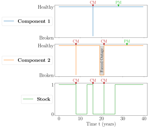
Figure 2: Illustration of the dynamics of a system with two components. When a failure occurs, if a spare part is available, a CM is performed immediately. The stock is then empty until the arrival of a new part (ordered at the time of the previous failure). If a failure occurs and the stock is empty, there is a forced outage until the arrival of a spare part. Some PMs can be performed to avoid failures, they do not use parts from the stock as they can be scheduled in advance.

The model intends to represent the following real situations:

1. In a single production unit, we consider a system with a unique family of components from the plant (either turbines, transformers or generators). In this case, any failure of a component induces a failure of the system (series system). In a real situation, the number of components in this case can be up to $10$.

2. We can also consider a system with components across several production units, still with one common stock. This time, a failure of a given component will only induce a failure of its own production unit and not of the whole system. Our methodology remains applicable to this system with the only difference that there is one forced outage cost for each unit. In this case the number of components can be up to $80$.

3. Finally, the developed methodology is also easily applicable to a system with several families of components and one separate stock of spares for each family. The components can be either in a single production unit or distributed across several units.

The primary goal of our work is to show that we are able to tackle maintenance scheduling problems with a large number of components (up to $80$). This is why, we design a model that is a proxy for the aforementioned cases. In Section 5, we explain how our model can be used to represent each of the three real situations described above.

2.1.1 Characterization of the stock and the components

The stock over time is characterized by the sequence of random variables

$$\boldsymbol{S^{\textstyle\text{\unboldmath$\scriptstyle$}}_{\textstyle\text{\unboldmath$\scriptstyle$}}}=(\boldsymbol{S^{\textstyle\text{\unboldmath$\scriptstyle$}}_{\textstyle\text{\unboldmath$\scriptstyle 0$}}},\ldots,\boldsymbol{S^{\textstyle\text{\unboldmath$\scriptstyle$}}_{\textstyle\text{\unboldmath$\scriptstyle T$}}})\in\mathcal{S}\;,$$ (2.3)

where $\boldsymbol{S^{\textstyle\text{\unboldmath$\scriptstyle$}}_{\textstyle\text{\unboldmath$\scriptstyle t$}}}:\Omega\rightarrow\{0,\ldots,s\}$ is the random variable representing the number of available spare parts at time $t$ and $\mathcal{S}$ is the set of all random variables taking values in $\{0,\ldots,s\}^{T+1}$. The parameter $s\in\mathbb{N}$ is the maximum number of spare parts. The value of the initial stock is set to $\boldsymbol{S^{\textstyle\text{\unboldmath$\scriptstyle$}}_{\textstyle\text{\unboldmath$\scriptstyle 0$}}}=s$. The replenishment delay for the parts, that is, the time from order to delivery of a part, is known and denoted by $D\in\mathbb{N}$.

At time $t$, component $i$ is characterized by random variables representing:

• its regime

  $$\boldsymbol{E^{\textstyle\text{\unboldmath$\scriptstyle$}}_{\textstyle\text{\unboldmath$\scriptstyle i,t$}}}=\left\{\begin{aligned} 0&\text{ if the component is broken},\\ 1&\text{ if the component is healthy}.\end{aligned}\right.$$ (2.4)

  A component has only two regimes: in the healthy regime, it runs in its nominal operating point. In the broken regime, it stops working completely. Initially all components are healthy i.e. $\boldsymbol{E^{\textstyle\text{\unboldmath$\scriptstyle$}}_{\textstyle\text{\unboldmath$\scriptstyle i,0$}}}=1$ for all $i\in\mathbb{I}$.

• its age (if healthy) or the time for which it has failed (if broken) denoted by the real-valued random variable $\boldsymbol{A^{\textstyle\text{\unboldmath$\scriptstyle$}}_{\textstyle\text{\unboldmath$\scriptstyle i,t$}}}$. Initially the components are new i.e. $\boldsymbol{A^{\textstyle\text{\unboldmath$\scriptstyle$}}_{\textstyle\text{\unboldmath$\scriptstyle i,0$}}}=0$ for all $i\in\mathbb{I}$.

• the time elapsed since its last $D$ failures

  $$\boldsymbol{P^{\textstyle\text{\unboldmath$\scriptstyle$}}_{\textstyle\text{\unboldmath$\scriptstyle i,t$}}}=(\boldsymbol{P^{\textstyle\text{\unboldmath$\scriptstyle 1$}}_{\textstyle\text{\unboldmath$\scriptstyle i,t$}}},\ldots,\boldsymbol{P^{\textstyle\text{\unboldmath$\scriptstyle D$}}_{\textstyle\text{\unboldmath$\scriptstyle i,t$}}})\;,$$ (2.5)

  where $D$ is the number of time steps for the supply of spare parts. For $d\in\{1,\ldots,D\},\ \boldsymbol{P^{\textstyle\text{\unboldmath$\scriptstyle d$}}_{\textstyle\text{\unboldmath$\scriptstyle i,t$}}}$ is the number of time steps elapsed since the $d$-th undiscarded failure of component $i$. $\boldsymbol{P^{\textstyle\text{\unboldmath$\scriptstyle d$}}_{\textstyle\text{\unboldmath$\scriptstyle i,t$}}}$ takes a default value $\delta$ if the component has failed fewer than $d$ times. Hence, $\boldsymbol{P^{\textstyle\text{\unboldmath$\scriptstyle d$}}_{\textstyle\text{\unboldmath$\scriptstyle i,t$}}}$ takes values in $\{\delta\}\cup\mathbb{R}_{+}$ and $\boldsymbol{P^{\textstyle\text{\unboldmath$\scriptstyle$}}_{\textstyle\text{\unboldmath$\scriptstyle i,0$}}}=(\delta,\ldots,\delta)$. The random vector $\boldsymbol{P^{\textstyle\text{\unboldmath$\scriptstyle$}}_{\textstyle\text{\unboldmath$\scriptstyle i,t$}}}$ is useful to compute the dates of replenishment of the stock. It is enough to store at most the dates of the last $D$ failures to describe the supply of the stock. More details are given in §2.2.1.

The characteristics of component $i$ at time $t$ are gathered in:

$$\boldsymbol{X^{\textstyle\text{\unboldmath$\scriptstyle$}}_{\textstyle\text{\unboldmath$\scriptstyle i,t$}}}=(\boldsymbol{E^{\textstyle\text{\unboldmath$\scriptstyle$}}_{\textstyle\text{\unboldmath$\scriptstyle i,t$}}},\boldsymbol{A^{\textstyle\text{\unboldmath$\scriptstyle$}}_{\textstyle\text{\unboldmath$\scriptstyle i,t$}}},\boldsymbol{P^{\textstyle\text{\unboldmath$\scriptstyle$}}_{\textstyle\text{\unboldmath$\scriptstyle i,t$}}})\in\mathcal{X}_{i,t}\;,$$ (2.6)

where $\mathcal{X}_{i,t}$ is the set of all random variables defined on $\Omega$ taking values in $\{0,1\}\times\mathbb{R}_{+}\times\left(\{\delta\}\cup\mathbb{R}_{+}\right)^{D}$. The state of the system is then described at $t$ by $(\boldsymbol{X^{\textstyle\text{\unboldmath$\scriptstyle$}}_{\textstyle\text{\unboldmath$\scriptstyle 1,t$}}},\ldots,\boldsymbol{X^{\textstyle\text{\unboldmath$\scriptstyle$}}_{\textstyle\text{\unboldmath$\scriptstyle n,t$}}},\boldsymbol{S^{\textstyle\text{\unboldmath$\scriptstyle$}}_{\textstyle\text{\unboldmath$\scriptstyle t$}}})$. Finally, to describe the components over the whole study period we introduce:

$$\boldsymbol{X^{\textstyle\text{\unboldmath$\scriptstyle$}}_{\textstyle\text{\unboldmath$\scriptstyle$}}}=(\boldsymbol{X^{\textstyle\text{\unboldmath$\scriptstyle$}}_{\textstyle\text{\unboldmath$\scriptstyle 1$}}},\ldots,\boldsymbol{X^{\textstyle\text{\unboldmath$\scriptstyle$}}_{\textstyle\text{\unboldmath$\scriptstyle n$}}})=((\boldsymbol{X^{\textstyle\text{\unboldmath$\scriptstyle$}}_{\textstyle\text{\unboldmath$\scriptstyle 1,0$}}},\ldots,\boldsymbol{X^{\textstyle\text{\unboldmath$\scriptstyle$}}_{\textstyle\text{\unboldmath$\scriptstyle 1,T$}}}),\ldots,(\boldsymbol{X^{\textstyle\text{\unboldmath$\scriptstyle$}}_{\textstyle\text{\unboldmath$\scriptstyle n,0$}}},\ldots,\boldsymbol{X^{\textstyle\text{\unboldmath$\scriptstyle$}}_{\textstyle\text{\unboldmath$\scriptstyle n,T$}}}))\in\mathcal{X}\;,$$ (2.7)

where $\mathcal{X}=\prod_{i=1}^{n}\mathcal{X}_{i}$ and $\mathcal{X}_{i}=\prod_{t=0}^{T}\mathcal{X}_{i,t}$, for all $i\in\mathbb{I}$. In order to emphasize that $\boldsymbol{X^{\textstyle\text{\unboldmath$\scriptstyle$}}_{\textstyle\text{\unboldmath$\scriptstyle$}}}$ depends on all the components of the system, we sometimes use the notation $\boldsymbol{X^{\textstyle\text{\unboldmath$\scriptstyle$}}_{\textstyle\text{\unboldmath$\scriptstyle 1:n$}}}$ instead of $\boldsymbol{X^{\textstyle\text{\unboldmath$\scriptstyle$}}_{\textstyle\text{\unboldmath$\scriptstyle$}}}$.

2.1.2 Preventive maintenance strategy

A PM consists in repairing a component although it is in the healthy regime. The dates of PM can be different for each component. They define the preventive maintenance strategy of the system. Operational constraints impose to look for deterministic strategies. This means that the dates of PM are chosen without any knowledge on the state of the system after the beginning of the time horizon and cannot be changed during the study. The maintenance strategy is defined by a vector

$$u=(u_{1},\ldots,u_{n})=((u_{1,0},\ldots,u_{1,T-1}),\ldots,(u_{n,0},\ldots,u_{n,T-1}))\in\mathbb{U}=[0,1]^{nT}\;,$$ (2.8)

where $u_{i,t}$ characterizes the PM for component $i$ at time $t$. More precisely, we set a threshold $0<\nu<1$: a control $u_{i,t}\geq\nu$ corresponds to a rejuvenation of the component proportional to $u_{i,t}$ and a value $u_{i,t}<\nu$ corresponds to not performing a maintenance. We consider that the duration of the maintenance operation is negligible. Moreover, a PM does not use parts from the stock as it is planned in advance and the parts are ordered so that they arrive just on time for the maintenance. Note that the modeling of the PM strategy uses a continuous decision variable $u$, this choice is justified in §2.5.

2.1.3 Failures of the components

In our study, the distribution of the time to failure for component $i$ is a known Weibull distribution with cumulative distribution function denoted by $F_{i}$. If component $i$ is healthy at time $t$ and has age $a\geq 0$ , its probability of failure at time $t+\Delta t$ is given by:

$$p_{i}(a)=\frac{F_{i}(a+\Delta t)-F_{i}(a)}{1-F_{i}(a)}\;.$$ (2.9)

We introduce the random sequence:

$$\boldsymbol{W^{\textstyle\text{\unboldmath$\scriptstyle$}}_{\textstyle\text{\unboldmath$\scriptstyle$}}}=(\boldsymbol{W^{\textstyle\text{\unboldmath$\scriptstyle$}}_{\textstyle\text{\unboldmath$\scriptstyle 1$}}},\ldots,\boldsymbol{W^{\textstyle\text{\unboldmath$\scriptstyle$}}_{\textstyle\text{\unboldmath$\scriptstyle n$}}})=((\boldsymbol{W^{\textstyle\text{\unboldmath$\scriptstyle$}}_{\textstyle\text{\unboldmath$\scriptstyle 1,1$}}},\ldots,\boldsymbol{W^{\textstyle\text{\unboldmath$\scriptstyle$}}_{\textstyle\text{\unboldmath$\scriptstyle 1,T$}}}),\ldots,(\boldsymbol{W^{\textstyle\text{\unboldmath$\scriptstyle$}}_{\textstyle\text{\unboldmath$\scriptstyle n,1$}}},\ldots,\boldsymbol{W^{\textstyle\text{\unboldmath$\scriptstyle$}}_{\textstyle\text{\unboldmath$\scriptstyle n,T$}}}))\in\mathcal{W}\;,$$ (2.10)

where $\mathcal{W}$ is the set of all random variables defined on $\Omega$ taking values in $[0,1]^{nT}$. The random process $\boldsymbol{W^{\textstyle\text{\unboldmath$\scriptstyle$}}_{\textstyle\text{\unboldmath$\scriptstyle$}}}$ is an exogenous noise that affects the dynamics of the regime $\boldsymbol{E^{\textstyle\text{\unboldmath$\scriptstyle$}}_{\textstyle\text{\unboldmath$\scriptstyle$}}}$ and the age $\boldsymbol{A^{\textstyle\text{\unboldmath$\scriptstyle$}}_{\textstyle\text{\unboldmath$\scriptstyle$}}}$. We assume that all $\boldsymbol{W^{\textstyle\text{\unboldmath$\scriptstyle$}}_{\textstyle\text{\unboldmath$\scriptstyle i,t$}}}$ are independent random variables and follow a uniform distribution on $[0,1]$. At time step $t$, component $i$ has age $\boldsymbol{A^{\textstyle\text{\unboldmath$\scriptstyle$}}_{\textstyle\text{\unboldmath$\scriptstyle i,t$}}}$. If $\boldsymbol{W^{\textstyle\text{\unboldmath$\scriptstyle$}}_{\textstyle\text{\unboldmath$\scriptstyle i,t+1$}}}<p_{i}(\boldsymbol{A^{\textstyle\text{\unboldmath$\scriptstyle$}}_{\textstyle\text{\unboldmath$\scriptstyle i,t$}}})$, component $i$ fails at $t+1$, otherwise no failure occurs.

2.2 Dynamics of the system

Now, we describe the dynamics of the system, that is, we explain how the variables characterizing the system evolve between two time steps.

2.2.1 Dynamics of a component

Let $i\in\mathbb{I}$ and $t\in\mathbb{T}_{-1}$. The dynamics of component $i$ between $t$ and $t+1$ is described as follows.

1. If component $i$ is healthy i.e. $\boldsymbol{E^{\textstyle\text{\unboldmath$\scriptstyle$}}_{\textstyle\text{\unboldmath$\scriptstyle i,t$}}}=1$:

   1. If $u_{i,t}\geq\nu$, then a PM is performed. After a PM, component $i$ stays healthy and is rejuvenated so that:

      $$(\boldsymbol{E^{\textstyle\text{\unboldmath$\scriptstyle$}}_{\textstyle\text{\unboldmath$\scriptstyle i,t+1$}}},\boldsymbol{A^{\textstyle\text{\unboldmath$\scriptstyle$}}_{\textstyle\text{\unboldmath$\scriptstyle i,t+1$}}})=(1,(1-u_{i,t})\boldsymbol{A^{\textstyle\text{\unboldmath$\scriptstyle$}}_{\textstyle\text{\unboldmath$\scriptstyle i,t$}}}+1)\;.$$ (2.11)

      The PM is performed instantaneously at time $t$, so after the maintenance (still at time $t$) its age is $(1-u_{i,t})\boldsymbol{A^{\textstyle\text{\unboldmath$\scriptstyle$}}_{\textstyle\text{\unboldmath$\scriptstyle i,t$}}}$. Therefore, the age is $(1-u_{i,t})\boldsymbol{A^{\textstyle\text{\unboldmath$\scriptstyle$}}_{\textstyle\text{\unboldmath$\scriptstyle i,t$}}}+1$ at time $t+1$. Note that $u_{i,t}=1$ makes the component as good as new: in this case we have $\boldsymbol{A^{\textstyle\text{\unboldmath$\scriptstyle$}}_{\textstyle\text{\unboldmath$\scriptstyle i,t+1$}}}=1$.

   2. If $u_{i,t}<\nu$, then no PM is performed. Component $i$ fails with probability $p_{i}(\boldsymbol{A^{\textstyle\text{\unboldmath$\scriptstyle$}}_{\textstyle\text{\unboldmath$\scriptstyle i,t$}}})$:

      $$(\boldsymbol{E^{\textstyle\text{\unboldmath$\scriptstyle$}}_{\textstyle\text{\unboldmath$\scriptstyle i,t+1$}}},\boldsymbol{A^{\textstyle\text{\unboldmath$\scriptstyle$}}_{\textstyle\text{\unboldmath$\scriptstyle i,t+1$}}})=\left\{\begin{aligned} &(0,0)&&\text{ if }\boldsymbol{W^{\textstyle\text{\unboldmath$\scriptstyle$}}_{\textstyle\text{\unboldmath$\scriptstyle i,t+1$}}}<p_{i}(\boldsymbol{A^{\textstyle\text{\unboldmath$\scriptstyle$}}_{\textstyle\text{\unboldmath$\scriptstyle i,t$}}})\;,\\ &(1,\boldsymbol{A^{\textstyle\text{\unboldmath$\scriptstyle$}}_{\textstyle\text{\unboldmath$\scriptstyle i,t$}}}+1)&&\text{ otherwise}\;.\end{aligned}\right.$$ (2.12)

2. If component $i$ is broken i.e. $\boldsymbol{E^{\textstyle\text{\unboldmath$\scriptstyle$}}_{\textstyle\text{\unboldmath$\scriptstyle i,t$}}}=0$:

   1. If a spare is available in the stock, a CM is performed to replace the component. We assume that the CM is an identical replacement, which implies that the component becomes as good as new. We get:

      $$(\boldsymbol{E^{\textstyle\text{\unboldmath$\scriptstyle$}}_{\textstyle\text{\unboldmath$\scriptstyle i,t+1$}}},\boldsymbol{A^{\textstyle\text{\unboldmath$\scriptstyle$}}_{\textstyle\text{\unboldmath$\scriptstyle i,t+1$}}})=(1,1)\;.$$ (2.13)

      A CM is performed instantaneously at time $t$, so the age of the component is $0$ after the CM, therefore it has age $1$ at time $t+1$.

   2. If no spare part is available, the defective component stays in the broken regime:

      $$(\boldsymbol{E^{\textstyle\text{\unboldmath$\scriptstyle$}}_{\textstyle\text{\unboldmath$\scriptstyle i,t+1$}}},\boldsymbol{A^{\textstyle\text{\unboldmath$\scriptstyle$}}_{\textstyle\text{\unboldmath$\scriptstyle i,t+1$}}})=(0,\boldsymbol{A^{\textstyle\text{\unboldmath$\scriptstyle$}}_{\textstyle\text{\unboldmath$\scriptstyle i,t$}}}+1)\;.$$ (2.14)

      As all components belong to the same power plant, when at least one component is broken, the unit is shut down until the arrival of a spare part and the execution of the CM. Such a situation is a forced outage. During the shut down no electricity is produced.

We have to express formally that a spare part is available for the replacement of component $i$. At time $t$, suppose that the stock has $\boldsymbol{S^{\textstyle\text{\unboldmath$\scriptstyle$}}_{\textstyle\text{\unboldmath$\scriptstyle t$}}}=r$ parts and that $m$ components are broken. If $r\geq m$, then all components can be replaced immediately. When $r<m$, we must choose which components to replace. Our modeling choice is to replace the broken components following the order of their index: if $i_{1}\leq\ldots\leq i_{r}\leq\ldots\leq i_{m}$ are the indices of the broken components, we replace only the components with index $i_{1},\ldots,i_{r}$, the others stay in the broken regime and wait for new available parts. Using this choice, the availability of a spare part for component $i$ corresponds to the condition:

$$\boldsymbol{S^{\textstyle\text{\unboldmath$\scriptstyle$}}_{\textstyle\text{\unboldmath$\scriptstyle t$}}}\geq\sum_{j=1}^{i}\mathbf{1}_{\{0\}}(\boldsymbol{E^{\textstyle\text{\unboldmath$\scriptstyle$}}_{\textstyle\text{\unboldmath$\scriptstyle j,t$}}})\;.$$ (2.15)

The right hand side of (2.15) simply counts the number of broken components with index smaller or equal than $i$.

To completely describe the dynamics of a component, we have to specify the dynamics of the vector $\boldsymbol{P^{\textstyle\text{\unboldmath$\scriptstyle$}}_{\textstyle\text{\unboldmath$\scriptstyle i,t$}}}$. It has been introduced in §2.1.1 to store the dates of failures of the component and compute the dates for the replenishment of the stock.

• If $\boldsymbol{P^{\textstyle\text{\unboldmath$\scriptstyle$}}_{\textstyle\text{\unboldmath$\scriptstyle i,t$}}}=(t_{1},\ldots,t_{d},\delta,\ldots,\delta)$ with $t_{1},\ldots,t_{d}\geq 0$, meaning that component $i$ has undergone $d<D$ failures so far, then:

  $$(t_{1}+1,\ldots,t_{d}+1,0,\delta,\ldots,\delta) \text{if failure at $t+1$}\;,$$ (2.16a)

  $$(t_{1}+1,\ldots,t_{d}+1,\delta,\delta,\ldots,\delta) \text{otherwise}\;.$$ (2.16b)

• If $\boldsymbol{P^{\textstyle\text{\unboldmath$\scriptstyle$}}_{\textstyle\text{\unboldmath$\scriptstyle i,t$}}}=(t_{1},\ldots,t_{D})$ with $t_{1},\ldots,t_{D}\geq 0$, meaning that component $i$ has undergone at least $D$ failures so far, then:

  $$(t_{2}+1,\ldots,t_{D}+1,0) \text{if failure at $t+1$}\;,$$ (2.17a)

  $$(t_{1}+1,\ldots,t_{D}+1) \text{otherwise}\;.$$ (2.17b)

  In (2.17a), note that $t_{1}$ is discarded. As $\boldsymbol{P^{\textstyle\text{\unboldmath$\scriptstyle$}}_{\textstyle\text{\unboldmath$\scriptstyle i,t$}}}=(t_{1},\ldots,t_{D})$ and $t_{1}>\ldots>t_{D}\geq 0$, we get that $t_{1}\geq D-1$. At time step $t+1$, the part ordered from the failure at $t_{1}$ has arrived. Then, storing $t_{1}$ is not useful anymore. So if a failure occurs at $t+1$, we can discard $t_{1}$ to make room for the new date of failure. This proves that it is enough to have $\boldsymbol{P^{\textstyle\text{\unboldmath$\scriptstyle$}}_{\textstyle\text{\unboldmath$\scriptstyle i,t$}}}$ of size $D$ to compute the replenishment of the stock as stated in §2.1.1. Note that the dates are not discarded if there is no failure (see (2.17b)), so it is possible to have $t_{d}>D$ for some $d\in\{1,\ldots,D\}$. Such variables have no influence on the dynamics of the system.

Figure 3: Dynamics of component $i$.

In Fig. 3, we summarize the dynamics of component $i$ from $t$ to $t+1$. Recall that we have $\boldsymbol{X^{\textstyle\text{\unboldmath$\scriptstyle$}}_{\textstyle\text{\unboldmath$\scriptstyle i,t$}}}=(\boldsymbol{E^{\textstyle\text{\unboldmath$\scriptstyle$}}_{\textstyle\text{\unboldmath$\scriptstyle i,t$}}},\boldsymbol{A^{\textstyle\text{\unboldmath$\scriptstyle$}}_{\textstyle\text{\unboldmath$\scriptstyle i,t$}}},\boldsymbol{P^{\textstyle\text{\unboldmath$\scriptstyle$}}_{\textstyle\text{\unboldmath$\scriptstyle i,t$}}})$. We write the dynamics of component $i$ on the whole time horizon as:

$$\Theta_{i}(\boldsymbol{X^{\textstyle\text{\unboldmath$\scriptstyle$}}_{\textstyle\text{\unboldmath$\scriptstyle 1:i$}}},\boldsymbol{S^{\textstyle\text{\unboldmath$\scriptstyle$}}_{\textstyle\text{\unboldmath$\scriptstyle$}}},u_{i},\boldsymbol{W^{\textstyle\text{\unboldmath$\scriptstyle$}}_{\textstyle\text{\unboldmath$\scriptstyle i$}}})=0\;,$$ (2.18)

where $\Theta_{i}=\{\Theta_{i,t}\}_{t\in\mathbb{T}}$ is such that:

$$\left\{\begin{aligned} \Theta_{i,t+1}(\boldsymbol{X^{\textstyle\text{\unboldmath$\scriptstyle$}}_{\textstyle\text{\unboldmath$\scriptstyle 1:i$}}},\boldsymbol{S^{\textstyle\text{\unboldmath$\scriptstyle$}}_{\textstyle\text{\unboldmath$\scriptstyle$}}},u_{i},\boldsymbol{W^{\textstyle\text{\unboldmath$\scriptstyle$}}_{\textstyle\text{\unboldmath$\scriptstyle i$}}})&=\boldsymbol{X^{\textstyle\text{\unboldmath$\scriptstyle$}}_{\textstyle\text{\unboldmath$\scriptstyle i,t+1$}}}-f_{i}(\boldsymbol{X^{\textstyle\text{\unboldmath$\scriptstyle$}}_{\textstyle\text{\unboldmath$\scriptstyle 1:i,t$}}},\boldsymbol{S^{\textstyle\text{\unboldmath$\scriptstyle$}}_{\textstyle\text{\unboldmath$\scriptstyle t$}}},u_{i,t},\boldsymbol{W^{\textstyle\text{\unboldmath$\scriptstyle$}}_{\textstyle\text{\unboldmath$\scriptstyle i,t+1$}}}),\quad t\in\mathbb{T}_{-1}\;,\\ \Theta_{i,0}(\boldsymbol{X^{\textstyle\text{\unboldmath$\scriptstyle$}}_{\textstyle\text{\unboldmath$\scriptstyle 1:i$}}},\boldsymbol{S^{\textstyle\text{\unboldmath$\scriptstyle$}}_{\textstyle\text{\unboldmath$\scriptstyle$}}},u_{i},\boldsymbol{W^{\textstyle\text{\unboldmath$\scriptstyle$}}_{\textstyle\text{\unboldmath$\scriptstyle i$}}})&=\boldsymbol{X^{\textstyle\text{\unboldmath$\scriptstyle$}}_{\textstyle\text{\unboldmath$\scriptstyle i,0$}}}-x_{i}\;,\enspace\end{aligned}\right.$$ (2.19)

with $x_{i}=(1,0,\delta,\ldots,\delta)^{\top}$ and $f_{i}$ represents the dynamics we just described for component $i$. An explicit expression of $f_{i}$ is given in Appendix A.

Note that there is a coupling between the dynamics of component $i$ and the stock. There is also a coupling with components $j<i$. This is due to the choice (2.15) of replacing the broken components with the smallest indices first if there are not enough spare parts.

2.2.2 Dynamics of the stock

For the stock, the initial number of spare parts is $\boldsymbol{S^{\textstyle\text{\unboldmath$\scriptstyle$}}_{\textstyle\text{\unboldmath$\scriptstyle 0$}}}=s$. As PMs can be anticipated, we consider that the required spares are ordered so that they arrive just on time for the scheduled maintenance. Therefore, they do not appear in the dynamics of the stock. A part is used for each CM and a new part is ordered only after the failure of a component. The number of time steps for the supply of a part is $D$. Hence, the part ordered after the $d$-th undiscarded failure of component $i$ arrives in the stock at $t+1$ if $\boldsymbol{P^{\textstyle\text{\unboldmath$\scriptstyle d$}}_{\textstyle\text{\unboldmath$\scriptstyle i,t+1$}}}=D$. This is equivalent to $\boldsymbol{P^{\textstyle\text{\unboldmath$\scriptstyle d$}}_{\textstyle\text{\unboldmath$\scriptstyle i,t$}}}=D-1$. On the other hand, the number of broken components is $\sum_{i=1}^{n}\mathbf{1}_{\{0\}}(\boldsymbol{E^{\textstyle\text{\unboldmath$\scriptstyle$}}_{\textstyle\text{\unboldmath$\scriptstyle i,t$}}})$ and we replace as many of them as possible given the current level of stock $\boldsymbol{S^{\textstyle\text{\unboldmath$\scriptstyle$}}_{\textstyle\text{\unboldmath$\scriptstyle t$}}}$. Thus, we have:

$$\boldsymbol{S^{\textstyle\text{\unboldmath$\scriptstyle$}}_{\textstyle\text{\unboldmath$\scriptstyle t+1$}}}=\boldsymbol{S^{\textstyle\text{\unboldmath$\scriptstyle$}}_{\textstyle\text{\unboldmath$\scriptstyle t$}}}+\sum_{i=1}^{n}\sum_{d=1}^{D}\mathbf{1}_{\{D-1\}}(\boldsymbol{P^{\textstyle\text{\unboldmath$\scriptstyle d$}}_{\textstyle\text{\unboldmath$\scriptstyle i,t$}}})-\min\left\{\boldsymbol{S^{\textstyle\text{\unboldmath$\scriptstyle$}}_{\textstyle\text{\unboldmath$\scriptstyle t$}}},\ \sum_{i=1}^{n}\mathbf{1}_{\{0\}}(\boldsymbol{E^{\textstyle\text{\unboldmath$\scriptstyle$}}_{\textstyle\text{\unboldmath$\scriptstyle i,t$}}})\right\},\quad t\in\mathbb{T}_{-1}\;.$$ (2.20)

We write the dynamics of the stock in compact form as:

$$\Theta_{\boldsymbol{S^{\textstyle\text{\unboldmath$\scriptstyle$}}_{\textstyle\text{\unboldmath$\scriptstyle$}}}}(\boldsymbol{X^{\textstyle\text{\unboldmath$\scriptstyle$}}_{\textstyle\text{\unboldmath$\scriptstyle 1:n$}}},\boldsymbol{S^{\textstyle\text{\unboldmath$\scriptstyle$}}_{\textstyle\text{\unboldmath$\scriptstyle$}}})=0\;,$$ (2.21)

where $\Theta_{\boldsymbol{S^{\textstyle\text{\unboldmath$\scriptstyle$}}_{\textstyle\text{\unboldmath$\scriptstyle$}}}}=\{\Theta_{\boldsymbol{S^{\textstyle\text{\unboldmath$\scriptstyle$}}_{\textstyle\text{\unboldmath$\scriptstyle$}}},t}\}_{t\in\mathbb{T}}$ is such that:

$$\left\{\begin{aligned} \Theta_{\boldsymbol{S^{\textstyle\text{\unboldmath$\scriptstyle$}}_{\textstyle\text{\unboldmath$\scriptstyle$}}},t+1}(\boldsymbol{X^{\textstyle\text{\unboldmath$\scriptstyle$}}_{\textstyle\text{\unboldmath$\scriptstyle 1:n$}}},\boldsymbol{S^{\textstyle\text{\unboldmath$\scriptstyle$}}_{\textstyle\text{\unboldmath$\scriptstyle$}}})&=\boldsymbol{S^{\textstyle\text{\unboldmath$\scriptstyle$}}_{\textstyle\text{\unboldmath$\scriptstyle t+1$}}}-f_{\boldsymbol{S^{\textstyle\text{\unboldmath$\scriptstyle$}}_{\textstyle\text{\unboldmath$\scriptstyle$}}}}(\boldsymbol{X^{\textstyle\text{\unboldmath$\scriptstyle$}}_{\textstyle\text{\unboldmath$\scriptstyle 1:n,t$}}},\boldsymbol{S^{\textstyle\text{\unboldmath$\scriptstyle$}}_{\textstyle\text{\unboldmath$\scriptstyle t$}}}),\quad t\in\mathbb{T}_{-1}\;,\\ \Theta_{\boldsymbol{S^{\textstyle\text{\unboldmath$\scriptstyle$}}_{\textstyle\text{\unboldmath$\scriptstyle$}}},0}(\boldsymbol{X^{\textstyle\text{\unboldmath$\scriptstyle$}}_{\textstyle\text{\unboldmath$\scriptstyle 1:n$}}},\boldsymbol{S^{\textstyle\text{\unboldmath$\scriptstyle$}}_{\textstyle\text{\unboldmath$\scriptstyle$}}})&=\boldsymbol{S^{\textstyle\text{\unboldmath$\scriptstyle$}}_{\textstyle\text{\unboldmath$\scriptstyle 0$}}}-s\;,\enspace\end{aligned}\right.$$

with $f_{S}$ corresponding to the right-hand side of (2.20). Note that $\boldsymbol{S^{\textstyle\text{\unboldmath$\scriptstyle$}}_{\textstyle\text{\unboldmath$\scriptstyle t+1$}}}$ depends on on the current level of stock $\boldsymbol{S^{\textstyle\text{\unboldmath$\scriptstyle$}}_{\textstyle\text{\unboldmath$\scriptstyle t$}}}$ but also on $\boldsymbol{X^{\textstyle\text{\unboldmath$\scriptstyle$}}_{\textstyle\text{\unboldmath$\scriptstyle i,t$}}}$ for all $i\in\mathbb{I}$. The stock is coupling all the components of the system.

Finally, the dynamics of the whole system is summarized by the almost sure equality constraint $\Theta(\boldsymbol{X^{\textstyle\text{\unboldmath$\scriptstyle$}}_{\textstyle\text{\unboldmath$\scriptstyle$}}},\boldsymbol{S^{\textstyle\text{\unboldmath$\scriptstyle$}}_{\textstyle\text{\unboldmath$\scriptstyle$}}},u,\boldsymbol{W^{\textstyle\text{\unboldmath$\scriptstyle$}}_{\textstyle\text{\unboldmath$\scriptstyle$}}})=0$, where we have $\Theta:\mathcal{X}\times\mathcal{S}\times\mathbb{U}\times\mathcal{W}\rightarrow\mathcal{L}$, with $\Theta=\big{\{}\{\Theta_{i}\}_{i\in\mathbb{I}},\Theta_{\boldsymbol{S^{\textstyle\text{\unboldmath$\scriptstyle$}}_{\textstyle\text{\unboldmath$\scriptstyle$}}}}\big{\}}$ and $\mathcal{L}=\left(\prod_{i=1}^{n}\mathcal{L}_{i}\right)\times\mathcal{L}_{\boldsymbol{S^{\textstyle\text{\unboldmath$\scriptstyle$}}_{\textstyle\text{\unboldmath$\scriptstyle$}}}}$ where $\mathcal{L}_{i}$ is the set of random variables with range in $\mathbb{R}^{(D+2)(T+1)}$ and $\mathcal{L}_{\boldsymbol{S^{\textstyle\text{\unboldmath$\scriptstyle$}}_{\textstyle\text{\unboldmath$\scriptstyle$}}}}$ is the set of random variables with range in $\mathbb{R}^{(T+1)}$.

We have now completely described the dynamics of the system. In the next part we specify the costs associated to the system.

2.3 Costs generated by the system

The costs generated by the system are due to PMs, CMs and forced outages of the unit. In practice as PMs are scheduled in advance, they are cheaper than unpredictable CMs. A forced outage of the unit induces a loss of production. It is characterized by a yearly cost which is higher than that of a PM or a CM. We consider a discount rate $\tau$ meaning that a cost $c$ occurring at time $t$ will be valued $\eta_{t}c$ with the discount factor $\eta_{t}:=\frac{1}{(1+\tau)^{t}}.$ We introduce the following notations:

• $j^{P}_{i,t}(u_{i,t})$ is the PM cost incurred at time $t$ for component $i$. Let $C^{P}_{i}$ be the cost of a PM operation on component $i$. We set:

  $$j^{P}_{i,t}(u_{i,t})=\eta_{t}C^{P}_{i}u_{i,t}^{2}\;.$$ (2.22)

  We use a quadratic cost as it is strongly convex and should favor numerical convergence. In particular, in the case where $0<u_{i,t}<\nu$, which models a situation where no PM is performed, we have $j^{P}_{i,t}(u_{i,t})>0$.

• $j^{C}_{i,t}(\boldsymbol{X^{\textstyle\text{\unboldmath$\scriptstyle$}}_{\textstyle\text{\unboldmath$\scriptstyle i,t$}}})$ is the CM cost. It is due at the time of the failure of a component, even if there is no spare part to perform the operation immediately. Hence it only occurs when $(\boldsymbol{E^{\textstyle\text{\unboldmath$\scriptstyle$}}_{\textstyle\text{\unboldmath$\scriptstyle i,t$}}},\boldsymbol{A^{\textstyle\text{\unboldmath$\scriptstyle$}}_{\textstyle\text{\unboldmath$\scriptstyle i,t$}}})=(0,0)$. Let $C^{C}_{i}$ be the cost of a CM operation on component $i$. We have:

  $$j^{C}_{i,t}(\boldsymbol{X^{\textstyle\text{\unboldmath$\scriptstyle$}}_{\textstyle\text{\unboldmath$\scriptstyle i,t$}}})=\eta_{t}C^{C}_{i}\mathbf{1}_{\{0\}}(\boldsymbol{E^{\textstyle\text{\unboldmath$\scriptstyle$}}_{\textstyle\text{\unboldmath$\scriptstyle i,t$}}})\mathbf{1}_{\{0\}}(\boldsymbol{A^{\textstyle\text{\unboldmath$\scriptstyle$}}_{\textstyle\text{\unboldmath$\scriptstyle i,t$}}})\;.$$ (2.23)

• $j^{F}_{t}(\boldsymbol{X^{\textstyle\text{\unboldmath$\scriptstyle$}}_{\textstyle\text{\unboldmath$\scriptstyle 1:n,t$}}})$ is the forced outage cost. As all components belong to the same production unit, a forced outage occurs when at least one component is in a failed state and the CM has not been performed immediately because of a lack of spare part. Let $C^{F}$ be the forced outage cost per time unit. We have:

  $$j^{F}_{t}(\boldsymbol{X^{\textstyle\text{\unboldmath$\scriptstyle$}}_{\textstyle\text{\unboldmath$\scriptstyle 1:n,t$}}})=\eta_{t}C^{F}\min\left\{1,\ \sum_{i=1}^{n}\mathbf{1}_{\{0\}}(\boldsymbol{E^{\textstyle\text{\unboldmath$\scriptstyle$}}_{\textstyle\text{\unboldmath$\scriptstyle i,t$}}})\mathbf{1}_{\mathbb{R}_{+}^{*}}(\boldsymbol{A^{\textstyle\text{\unboldmath$\scriptstyle$}}_{\textstyle\text{\unboldmath$\scriptstyle i,t$}}})\right\}\;.$$ (2.24)

In order to consider the previous costs over the whole study period we introduce:

• the total maintenance cost (preventive and corrective) generated by component $i\in\mathbb{I}$ on the studied period:

  $$j_{i}(\boldsymbol{X^{\textstyle\text{\unboldmath$\scriptstyle$}}_{\textstyle\text{\unboldmath$\scriptstyle i$}}},u_{i})=\sum_{t=0}^{T-1}j^{P}_{i,t}(u_{i,t})+\sum_{t=0}^{T}j^{C}_{i,t}(\boldsymbol{X^{\textstyle\text{\unboldmath$\scriptstyle$}}_{\textstyle\text{\unboldmath$\scriptstyle i,t$}}})\;,\enspace$$ (2.25)

• the total forced outage cost generated by the system during the studied period:

  $$j^{F}(\boldsymbol{X^{\textstyle\text{\unboldmath$\scriptstyle$}}_{\textstyle\text{\unboldmath$\scriptstyle 1:n$}}})=\sum_{t=0}^{T}j^{F}_{t}(\boldsymbol{X^{\textstyle\text{\unboldmath$\scriptstyle$}}_{\textstyle\text{\unboldmath$\scriptstyle 1:n,t$}}})\;,\enspace$$ (2.26)

2.4 Formulation of the maintenance optimization problem

The dynamics of the system is stochastic as it depends on the failure of the components, modelled by the random vector $\boldsymbol{W^{\textstyle\text{\unboldmath$\scriptstyle$}}_{\textstyle\text{\unboldmath$\scriptstyle$}}}$. The cost function is then stochastic as well. The objective is to find the deterministic maintenance strategy $u\in\mathbb{U}$ that minimizes the expected cost generated by the system over all failure scenarios. Hence, the industrial optimal maintenance scheduling problem is formulated as follows:

$$\min_{(\boldsymbol{X^{\textstyle\text{\unboldmath$\scriptstyle$}}_{\textstyle\text{\unboldmath$\scriptstyle$}}},\boldsymbol{S^{\textstyle\text{\unboldmath$\scriptstyle$}}_{\textstyle\text{\unboldmath$\scriptstyle$}}},u)\in\mathcal{X}\times\mathcal{S}\times\mathbb{U}} \ \mathbb{E}\Big{(}\sum_{i=1}^{n}j_{i}(\boldsymbol{X^{\textstyle\text{\unboldmath$\scriptstyle$}}_{\textstyle\text{\unboldmath$\scriptstyle i$}}},u_{i})+j^{F}(\boldsymbol{X^{\textstyle\text{\unboldmath$\scriptstyle$}}_{\textstyle\text{\unboldmath$\scriptstyle 1:n$}}})\Big{)}$$ (2.27)

$$\mathrm{s.t.} \ \Theta(\boldsymbol{X^{\textstyle\text{\unboldmath$\scriptstyle$}}_{\textstyle\text{\unboldmath$\scriptstyle$}}},\boldsymbol{S^{\textstyle\text{\unboldmath$\scriptstyle$}}_{\textstyle\text{\unboldmath$\scriptstyle$}}},u,\boldsymbol{W^{\textstyle\text{\unboldmath$\scriptstyle$}}_{\textstyle\text{\unboldmath$\scriptstyle$}}})=0\;,\quad\text{$\mathbb{P}$-}\text{a.s.}\;.$$

The term $\mathbb{E}(\sum_{i=1}^{n}j_{i}(\boldsymbol{X^{\textstyle\text{\unboldmath$\scriptstyle$}}_{\textstyle\text{\unboldmath$\scriptstyle i$}}},u_{i}))=\sum_{i=1}^{n}\mathbb{E}(j_{i}(\boldsymbol{X^{\textstyle\text{\unboldmath$\scriptstyle$}}_{\textstyle\text{\unboldmath$\scriptstyle i$}}},u_{i}))$ is additive with respect to the components whereas $\mathbb{E}(j^{F}(\boldsymbol{X^{\textstyle\text{\unboldmath$\scriptstyle$}}_{\textstyle\text{\unboldmath$\scriptstyle 1:n$}}}))$ induces a non-additive coupling between the components. In the theoretical part on the Auxiliary Problem Principle (Section 3), we will see that these two terms are treated in a different way for the design of a decomposition-coordination algorithm.

2.5 Complexity of the problem and limits of a direct approach

For maintenance scheduling problems that involve systems that are similar to the one considered in this paper, the algorithm MADS (Mesh Adaptive Direct Search) [7] can be used. In particular, MADS has been successfully applied for periodic maintenance problems in [4] and for a system with $4$ components and monthly maintenance decisions in [1]. However, the problem considered here with $80$ components and general maintenance strategies is more challenging than the two previous ones.

The industrial maintenance problem (2.27) is a non-smooth non-convex optimization problem. The number of components $n$ in the system can be up to $80$ and $T$ is $40$ years so $\mathbb{U}$ has dimension up to $nT=3200$ as we have one maintenance decision each year for each component. In §2.2, the dynamics is modelled with the vector $\Theta$, taking values in $\mathcal{L}=\mathbb{R}^{(n(D+2)+1)(T+1)}$. Hence, there are $(n(D+2)+1)(T+1)$ constraints in Problem (2.27) i.e. $13161$ contraints for the systems studied in Section 5 with a delay $D=2$ years for the supply in spare parts. However, any maintenance strategy $u\in\mathbb{U}$ is feasible, as we can always choose whether or not to do a PM for each component at each time step. The dynamics $\Theta$ then allows to compute the value of $\boldsymbol{X^{\textstyle\text{\unboldmath$\scriptstyle$}}_{\textstyle\text{\unboldmath$\scriptstyle$}}}$ and $\boldsymbol{S^{\textstyle\text{\unboldmath$\scriptstyle$}}_{\textstyle\text{\unboldmath$\scriptstyle$}}}$ given the strategy $u$ and the occurrences of failures modelled by $\boldsymbol{W^{\textstyle\text{\unboldmath$\scriptstyle$}}_{\textstyle\text{\unboldmath$\scriptstyle$}}}$.

As the problem is non-smooth, non-convex and in high dimension, it is challenging for any frontal resolution approach, including the algorithm MADS. MADS is a blackbox algorithm, meaning that evaluation points are chosen iteratively without using the gradients of the objective function, which may not even be defined. This feature is particularly appealing as the cost function is not differentiable. The algorithm has been initially designed for continuous optimization, therefore it uses the modeling of §2.1 and the cost functions described in §2.3. In particular, the PM strategies are modelled with a continuous decision variable. When the number of components is not too large, say $n<10$, the maintenance problem (2.27) is solved efficiently by MADS: the algorithm converges in around a minute. When the number of components is large, MADS needs more iterations to explore the high-dimensional space of solutions. As the volume of the search space grows exponentially with the number of components, MADS may not be able to find an effective maintenance strategy in reasonable time (less than a day) for the most demanding case with $80$ components.

To overcome the difficulty of MADS when dealing with large systems, we implement a decomposition of Problem (2.27) component by component.

3 The Auxiliary Problem Principle for decomposition

When performing optimization on a large scale system, that is, a system which is described by a large number of variables or constraints, the computation is often highly expensive either in time or in memory requirement (or both). The idea of decomposition is to formulate subproblems involving only smaller subsystems of the original large system. Each subproblem is easier to solve than the global optimization problem and provides its “local” solution. Then the goal of coordination is to ensure that gathering the local solutions leads to a global solution. Decomposition-coordination methods usually result in an iterative process alternating an optimization step on the subsystems and a coordination step that updates the subproblems.

The main advantage of decomposition is that the resolution of the small subproblems is faster than the original problem. More than that, the computational complexity of an optimization problem is often superlinear or even exponential in the size of the problem. Hence, the sum of the computational efforts required for the resolution of all subproblems will be lower than for the global problem, even if the resolution of the subproblems must be carried out multiple times. Another feature of decomposition methods is that they are naturally adapted to parallelization as each subproblem is independent. This leads to a reduction of computation time.

In this section, we introduce the general framework of the Auxiliary Problem Principle (APP) that allows us to formulate a decomposition-coordination scheme for the optimization problem (2.27). The APP has first been introduced in [13] as a unified framework for decomposition methods but also for other classical iterative algorithms. This principle casts the resolution of an optimization problem into the resolution of a sequence of auxiliary problems whose solutions converge to the solution of the original problem. Appropriate choices for the auxiliary problems lead to decomposition-coordination schemes.

Based on [10], we present the main ideas of the APP. Consider the following problem, which we call the master problem:

$$\min_{u\in U^{\mathrm{ad}}}J_{\Sigma}(u)+J_{\Delta}(u)\ \text{ such that }\ \Theta(u)\in-C\;,$$ (3.1)

where:

• $U^{\mathrm{ad}}$ is a non-empty, closed, convex subset of a Hilbert space $\mathbb{U}=\mathbb{U}_{1}\times\ldots\times\mathbb{U}_{N}$ and is decomposable as $U^{\mathrm{ad}}=U^{\mathrm{ad}}_{1}\times\cdots\times U^{\mathrm{ad}}_{N}$ where for all $i\in\mathbb{I},\ U^{\mathrm{ad}}_{i}\subset\mathbb{U}_{i}$ is a closed convex set;

• $C$ is a pointed closed convex cone of a Hilbert space $\mathscr{C}=\mathscr{C}_{1}\times\cdots\times\mathscr{C}_{N}$ and is decomposable as $C={C}_{1}\times\cdots\times{C}_{N}$ where for all $i\in\mathbb{I},\ C_{i}\subset\mathscr{C}_{i}$ is a closed convex cone;

• $J_{\Sigma}:\mathbb{U}\rightarrow\mathbb{R}$ and $J_{\Delta}:\mathbb{U}\rightarrow\mathbb{R}$ are convex and lower semi-continuous (l.s.c.). The function $J_{\Sigma}+J_{\Delta}$ is coercive on $U^{\mathrm{ad}}$. Moreover, $J_{\Delta}$ is differentiable and $J_{\Sigma}$ is additive with respect to the decomposition of the admissible space, so that we have for $u=(u_{1},\ldots,u_{N})\in U^{\mathrm{ad}}$ with $u_{i}\in U^{\mathrm{ad}}_{i}$ for all $i\in\mathbb{I}$:

  $$J_{\Sigma}(u)=\sum_{i=1}^{N}J_{\Sigma,i}(u_{i})\;;$$ (3.2)

  where $J_{\Sigma,i}:\mathbb{U}_{i}\rightarrow\mathbb{R}$.

• $\Theta:\mathbb{U}\rightarrow\mathscr{C}$ is differentiable and $C$-convex, meaning that:

  $$\forall u,v\in\mathbb{U},\forall\rho\in[0,1],\rho\Theta(u)+(1-\rho)\Theta(v)-\Theta(\rho u+(1-\rho)v)\in C\;.$$ (3.3)

  We write $\Theta(u)=(\Theta_{1}(u),\ldots,\Theta_{N}(u))$ with $\Theta_{i}:\mathbb{U}\rightarrow\mathscr{C}_{i}$ for $i\in\mathbb{I}$.

The goal of the APP is to turn the resolution of the master problem on $U^{\mathrm{ad}}$ into the resolution of subproblems on the sets $U^{\mathrm{ad}}_{i}$. In the master problem, there is a non-additive coupling in the cost due to $J_{\Delta}$ and a coupling in the constraint $\Theta$.

We present the APP for the special case of the decomposition by prediction. The construction of a decomposable auxiliary problem relies on the following points:

1. The decomposition of the admissible space $U^{\mathrm{ad}}=U^{\mathrm{ad}}_{1}\times\cdots\times U^{\mathrm{ad}}_{N}$ defines the subspace on which each subproblem is solved.

2. The decomposition of the cone $C={C}_{1}\times\cdots\times{C}_{N}$ specifies which part of the constraint is assigned to each subproblem.

Let $\bar{u}=(\bar{u}_{1},\ldots,\bar{u}_{N})\in\mathbb{U}$ and $\bar{\lambda}=(\bar{\lambda}_{1},\ldots,\bar{\lambda}_{N})\in C^{\star}$ the dual cone of $C$. We recall that:

$$C^{\star}=\{\lambda\in\mathscr{C}^{\star},\left\langle\lambda\>,\mu\right\rangle\geq 0\text{ for all }\mu\in\mathscr{C}\}\;,$$ (3.4)

with $\mathscr{C}^{\star}$ being the dual space of $\mathscr{C}$. Let $K$ be an auxiliary cost and $\Phi$ be an auxiliary dynamics satisfying the following properties:

• $K:\mathbb{U}\rightarrow\mathbb{R}$ is convex, l.s.c., differentiable and additive: $\displaystyle K(u)=\sum_{i=1}^{N}K_{i}(u_{i})$;

• $\Phi:\mathbb{U}\rightarrow\mathscr{C}$ is differentiable and block-diagonal: $\Phi(u)=\big{(}\Phi_{1}(u_{1}),\ldots,\Phi_{N}(u_{N})\big{)}$.

The auxiliary problem for the master problem (3.1) arising from the choice of $K$ and $\Phi$ is given by:

$$\min_{u\in U^{\mathrm{ad}}} K(u)+J_{\Sigma}(u)+\left\langle\nabla J_{\Delta}(\bar{u})-\nabla K(\bar{u})\>,u\right\rangle+\left\langle\bar{\lambda}\>,\big{(}\Theta^{\prime}(\bar{u})-\Phi^{\prime}(\bar{u})\big{)}\cdot u\right\rangle$$ (3.5)

$$\mathrm{s.t.}\ \Phi(u)-\Phi(\bar{u})+\Theta(\bar{u})\in-C\;.$$

Choosing $K$ additive and $\Phi$ block-diagonal ensures that Problem (3.5) decomposes in $N$ independent subproblems that can be solved in parallel. For $i\in\mathbb{I}$, the $i$-th subproblem is given by:

$$\min_{u_{i}\in U^{\mathrm{ad}}_{i}} \begin{multlined}K_{i}(u_{i})+J_{\Sigma,i}(u_{i})+\left\langle\nabla_{u_{i}}J_{\Delta}(\bar{u})-\nabla K_{i}(\bar{u}_{i})\>,u_{i}\right\rangle\\ -\left\langle\bar{\lambda}_{i}\>,\Phi_{i}^{\prime}(\bar{u}_{i})\cdot u_{i}\right\rangle+\sum_{j=1}^{N}\left\langle\bar{\lambda}_{j}\>,\partial_{u_{i}}\Theta_{j}(\bar{u})\cdot u_{i}\right\rangle\end{multlined}K_{i}(u_{i})+J_{\Sigma,i}(u_{i})+\left\langle\nabla_{u_{i}}J_{\Delta}(\bar{u})-\nabla K_{i}(\bar{u}_{i})\>,u_{i}\right\rangle\\ -\left\langle\bar{\lambda}_{i}\>,\Phi_{i}^{\prime}(\bar{u}_{i})\cdot u_{i}\right\rangle+\sum_{j=1}^{N}\left\langle\bar{\lambda}_{j}\>,\partial_{u_{i}}\Theta_{j}(\bar{u})\cdot u_{i}\right\rangle$$ (3.6)

$$\mathrm{s.t.}\ \Phi_{i}(u_{i})-\Phi_{i}(\bar{u}_{i})+\Theta_{i}(\bar{u})\in-C_{i}\;.$$

This subproblem only depends on $u_{i}\in U^{\mathrm{ad}}_{i}$ and inherits only the $i$-th component of the constraint.

Example 3.1.

Let $\bar{u}\in\mathbb{U}$. A canonical choice for the additive auxiliary cost function $K$ is:

$$K(u)=\sum_{i=1}^{N}K_{i}(u_{i})\ \text{ with }\ K_{i}(u_{i})=J_{\Delta}(\bar{u}_{1:i-1},u_{i},\bar{u}_{i+1:n})\;.$$ (3.7)

where $u_{i:j}=(u_{i},\ldots,u_{j})$ for $i\leq j$ and the convention that $u_{i:j}$ is empty if $j>i$. Similarly, a canonical choice for the block-diagonal auxiliary dynamics $\Phi$ is:

$$\Phi(u)=(\Phi_{1}(u_{1}),\ldots,\Phi_{N}(u_{N}))\ \text{ with }\ \Phi_{i}(u_{i})=\Theta_{i}(\bar{u}_{1:i-1},u_{i},\bar{u}_{i+1:n})\;.$$ (3.8)

The general idea is to construct the $i$-th term of the auxiliary function from the original function where only the $i$-th component is allowed to vary.

The following statement is the fundamental lemma for the theory of the APP.

Lemma 3.2.

Let $u^{\sharp}$ be a solution of the auxiliary problem (3.5) and $\lambda^{\sharp}$ be an optimal multiplier for its constraint. If $(u^{\sharp},\lambda^{\sharp})=(\bar{u},\bar{\lambda})$, then $u^{\sharp}$ is a solution of the master problem (3.1) and $\lambda^{\sharp}$ is an optimal multiplier for its constraint.

The proof consists in checking that if $(u^{\sharp},\lambda^{\sharp})=(\bar{u},\bar{\lambda})$, then $(u^{\sharp},\lambda^{\sharp})$ solves the variational inequalities that are satisfied by an optimal solution and an optimal multiplier of the master problem (3.1). More details can be found in [10, Section 4]. Lemma 3.2 suggests to use the APP fixed-point Algorithm 1.

1:0Let $(\bar{u},\bar{\lambda})=(u^{0},\lambda^{0})\in U^{\mathrm{ad}}\times C^{\star}$ and set $k=0$.

2:-1At iteration $k+1$:

• Solve the auxiliary problem (3.5). Let $u^{k+1}$ be a solution and $\lambda^{k+1}$ be an optimal multiplier for its constraint.

• Set $(\bar{u},\bar{\lambda})=(u^{k+1},\lambda^{k+1})$.

3:-2If the maximum number of iterations is reached or $\left\|u^{k+1}-u^{k}\right\|$ + $\left\|\lambda^{k+1}-\lambda^{k}\right\|$ is sufficiently small then stop, else $k\leftarrow k+1$ and go back to step 2.

Algorithm 1 APP fixed-point algorithm

A convergence result for Algorithm 1, is given in [14].

Theorem 3.3.

[14, Theorem 5.1 with $\epsilon=1$] Assume that:

• The admissible space $U^{\mathrm{ad}}$ is equal to the whole space $\mathbb{U}$,

• The constraints are equality constraints, that is $C=\{0\}$,

• $K(u)=\frac{1}{2}\left\langle u\>,\mathsf{K}u\right\rangle,\ J_{\Sigma}(u)=0,\ J_{\Delta}(u)=\frac{1}{2}\left\langle u\>,\mathsf{J}u\right\rangle+\left\langle\mathsf{j}\>,u\right\rangle$ where $\mathsf{K}$ and $\mathsf{J}$ are linear self-adjoint strongly monotone and Lipschitz continuous operators, $\mathsf{j}$ is a vector in $\mathbb{U}$, and $2\mathsf{K}-\mathsf{J}$ is assumed to be strongly monotone,

• $\Phi(u)=\mathsf{O}u,\ \Theta(u)=\mathsf{T}u+\mathsf{t}$ where the operators $\mathsf{O}$ and $\mathsf{T}$ are linear and surjective and $\mathsf{t}$ is a vector in $\mathscr{C}$,

• (Geometric condition) The operator $2\left(\mathsf{T}\mathsf{J}^{-1}\mathsf{O}^{\top}+\mathsf{O}\mathsf{J}^{-1}\mathsf{T}^{\top}\right)-\mathsf{T}\mathsf{J}^{-1}(2\mathsf{K}+\mathsf{J})\mathsf{J}^{-1}\mathsf{T}^{\top}$ is strongly monotone.

Then, the sequence $\big{\{}(u^{k},\lambda^{k})\big{\}}_{k\in\mathbb{N}}$ generated by the APP fixed-point algorithm converges strongly to the unique optimal solution $(u^{\sharp},\lambda^{\sharp})$ of the original problem (3.1).

In this section, we have studied a master optimization problem with couplings coming both from the part $J_{\Delta}$ of the cost function and the constraint $\Theta$. The APP allows to turn the resolution of the master problem into the iterative resolution of an auxiliary problem that is decomposable into independent subproblems of smaller size. In the next section, we present the application of the APP to solve the maintenance optimization problem described in Section 2.

4 Application of the APP for the industrial maintenance problem

The application of the APP to Problem (2.27) is done as follows:

1. We specify a decomposition of the admissible space and of the space of contraints (§4.1).

2. We construct an auxiliary problem that is adapted to the proposed decomposition using a suitable auxiliary cost and auxiliary dynamics (§4.2).

3. The industrial system involves integer variables whereas the APP is based on variational techniques. Therefore, we proceed to a continuous relaxation of the system in order to compute the gradients of the dynamics that appear in the auxiliary problem (§4.3).

4. We give the explicit formulation of the independent subproblems that arise from the decomposition of the auxiliary problem (§4.4).

5. We see that the subproblem on the stock is easy to solve numerically. We take advantage of this feature to design an efficient implementation of the APP fixed-point algorithm mixing a parallel and sequential strategy for the resolution of the subproblems (§4.5).

The APP fixed-point algorithm presented in §4.5 is then applied to numerical test cases in Section 5.

4.1 Decomposition of the space by component

We start by specifying the decomposition of the admissible space and of the cone of constraints that is considered for the design of the decomposition by component.

Considering the physical nature of the industrial system composed of $n$ components and a stock, we choose to decompose the problem in $n+1$ subproblems and call this decomposition a decomposition by component. More precisely, for $i\in\mathbb{I}$, the $i$-th subproblem is called subproblem on component $i$ since it is solved on $\mathcal{X}_{i}\times\mathbb{U}_{i}$ and only involves the dynamics of component $i$. The $(n+1)$-th subproblem is called subproblem on the stock since it is solved on $\mathcal{S}$ and only involves the dynamics of the stock. This means that the admissible space $\mathcal{X}\times\mathcal{S}\times\mathbb{U}$ of Problem (2.27) is decomposed as a product of a $n+1$ subspaces:

$$\mathcal{X}\times\mathcal{S}\times\mathbb{U}=(\mathcal{X}_{1}\times\mathbb{U}_{1})\times\ldots\times(\mathcal{X}_{n}\times\mathbb{U}_{n})\times\mathcal{S}\;,$$ (4.1)

where, for $(\boldsymbol{X^{\textstyle\text{\unboldmath$\scriptstyle$}}_{\textstyle\text{\unboldmath$\scriptstyle$}}},\boldsymbol{S^{\textstyle\text{\unboldmath$\scriptstyle$}}_{\textstyle\text{\unboldmath$\scriptstyle$}}},u)=((\boldsymbol{X^{\textstyle\text{\unboldmath$\scriptstyle$}}_{\textstyle\text{\unboldmath$\scriptstyle 1$}}},\ldots,\boldsymbol{X^{\textstyle\text{\unboldmath$\scriptstyle$}}_{\textstyle\text{\unboldmath$\scriptstyle n$}}}),\boldsymbol{S^{\textstyle\text{\unboldmath$\scriptstyle$}}_{\textstyle\text{\unboldmath$\scriptstyle$}}},(u_{1},\ldots,u_{n}))\in\mathcal{X}\times\mathcal{S}\times\mathbb{U}$, we have

$$(\boldsymbol{X^{\textstyle\text{\unboldmath$\scriptstyle$}}_{\textstyle\text{\unboldmath$\scriptstyle i$}}},u_{i})\in\mathcal{X}_{i}\times\mathbb{U}_{i}\text{ for all }i\in\mathbb{I}\text{ and }\boldsymbol{S^{\textstyle\text{\unboldmath$\scriptstyle$}}_{\textstyle\text{\unboldmath$\scriptstyle$}}}\in\mathcal{S}\;.$$ (4.2)

The constraints in Problem (2.27), that is $\Theta(\boldsymbol{X^{\textstyle\text{\unboldmath$\scriptstyle$}}_{\textstyle\text{\unboldmath$\scriptstyle$}}},\boldsymbol{S^{\textstyle\text{\unboldmath$\scriptstyle$}}_{\textstyle\text{\unboldmath$\scriptstyle$}}},u,\boldsymbol{W^{\textstyle\text{\unboldmath$\scriptstyle$}}_{\textstyle\text{\unboldmath$\scriptstyle$}}})\in-C$ with $C=\{0\}_{\mathcal{L}}$ is decomposed through the following cone decomposition:

$$C=\{0\}_{\mathcal{L}}=\{0\}_{\mathcal{L}_{1}}\times\ldots\times\{0\}_{\mathcal{L}_{n}}\times\{0\}_{\mathcal{L}_{\boldsymbol{S^{\textstyle\text{\unboldmath$\scriptstyle$}}_{\textstyle\text{\unboldmath$\scriptstyle$}}}}}=C_{1}\times\ldots C_{n}\times C_{\boldsymbol{S^{\textstyle\text{\unboldmath$\scriptstyle$}}_{\textstyle\text{\unboldmath$\scriptstyle$}}}}\;,$$ (4.3)

where for $i\in\mathbb{I},\ \{0\}_{\mathcal{L}_{i}},\{0\}_{\mathcal{L}_{\boldsymbol{S^{\textstyle\text{\unboldmath$\scriptstyle$}}_{\textstyle\text{\unboldmath$\scriptstyle$}}}}}$ and $\{0\}_{\mathcal{L}}$ denote the null function of $\mathcal{L}_{i},\mathcal{L}_{\boldsymbol{S^{\textstyle\text{\unboldmath$\scriptstyle$}}_{\textstyle\text{\unboldmath$\scriptstyle$}}}}$ and $\mathcal{L}$ respectively. We recall that $\Theta_{i}$ takes values in $\mathcal{L}_{i}$ and $\Theta_{\boldsymbol{S^{\textstyle\text{\unboldmath$\scriptstyle$}}_{\textstyle\text{\unboldmath$\scriptstyle$}}}}$ takes values in $\mathcal{L}_{\boldsymbol{S^{\textstyle\text{\unboldmath$\scriptstyle$}}_{\textstyle\text{\unboldmath$\scriptstyle$}}}}$.

4.2 Construction of an auxiliary problem

In this section, we choose the auxiliary functions that lead to the construction of a decomposable auxiliary problem.

Problem (2.27) is not directly decomposable by component because of couplings, highlighted in Section 2, that we recall now.

• The expected maintenance cost $\mathbb{E}(\sum_{i=1}^{n}j_{i}(\boldsymbol{X^{\textstyle\text{\unboldmath$\scriptstyle$}}_{\textstyle\text{\unboldmath$\scriptstyle i$}}},u_{i}))$ is additive with respect to the decomposition by component and can be identified with $J_{\Sigma}$ in Section 3.

• The forced outage cost $j^{F}$ induces a non-additive coupling between the components. The expected forced outage cost $\mathbb{E}(j^{F}(\boldsymbol{X^{\textstyle\text{\unboldmath$\scriptstyle$}}_{\textstyle\text{\unboldmath${}_{1:n}$}}}))$ can be identified with $J_{\Delta}$ in Section 3.

• The dynamics $\Theta_{i}$ of component $i$ induces a coupling with the stock and all components with index $j<i$. The stock dynamics, $\Theta_{\boldsymbol{S^{\textstyle\text{\unboldmath$\scriptstyle$}}_{\textstyle\text{\unboldmath$\scriptstyle$}}}}$, is coupling the stock with all components.

In order to obtain a decomposition of Problem (2.27) by component, we use the canonical technique from Example 3.8. We define an additive mapping $K$ and a block diagonal mapping $\Phi$ so that the resulting auxiliary problem is decomposable. We also choose to augment the auxiliary cost $K$ with a strongly convex term in order to ease the numerical convergence of the method. Let $\bar{\boldsymbol{X^{\textstyle\text{\unboldmath$\scriptstyle$}}_{\textstyle\text{\unboldmath$\scriptstyle$}}}}=(\bar{\boldsymbol{X^{\textstyle\text{\unboldmath$\scriptstyle$}}_{\textstyle\text{\unboldmath$\scriptstyle$}}}}_{1},\ldots,\bar{\boldsymbol{X^{\textstyle\text{\unboldmath$\scriptstyle$}}_{\textstyle\text{\unboldmath$\scriptstyle$}}}}_{n})\in\mathcal{X}$, $\bar{\boldsymbol{S^{\textstyle\text{\unboldmath$\scriptstyle$}}_{\textstyle\text{\unboldmath$\scriptstyle$}}}}\in\mathcal{S}$, $\bar{u}\in\mathbb{U}$, $\bar{\boldsymbol{\Lambda^{\textstyle\text{\unboldmath$\scriptstyle$}}_{\textstyle\text{\unboldmath$\scriptstyle$}}}}\in C^{\star}$ and $\gamma_{x},\gamma_{s},\gamma_{u}>0$. We consider:

• An additive auxiliary cost function $K:\mathcal{X}\times\mathcal{S}\times\mathbb{U}\rightarrow\mathbb{R}$:

  $$K(\boldsymbol{X^{\textstyle\text{\unboldmath$\scriptstyle$}}_{\textstyle\text{\unboldmath$\scriptstyle$}}},\boldsymbol{S^{\textstyle\text{\unboldmath$\scriptstyle$}}_{\textstyle\text{\unboldmath$\scriptstyle$}}},u)=\sum_{i=1}^{n}K_{i}(\boldsymbol{X^{\textstyle\text{\unboldmath$\scriptstyle$}}_{\textstyle\text{\unboldmath$\scriptstyle i$}}},u_{i})+K_{\boldsymbol{S^{\textstyle\text{\unboldmath$\scriptstyle$}}_{\textstyle\text{\unboldmath$\scriptstyle$}}}}(\boldsymbol{S^{\textstyle\text{\unboldmath$\scriptstyle$}}_{\textstyle\text{\unboldmath$\scriptstyle$}}})\;,$$ (4.4)

  with:

  $$K_{i}(\boldsymbol{X^{\textstyle\text{\unboldmath$\scriptstyle$}}_{\textstyle\text{\unboldmath$\scriptstyle i$}}},u_{i}) =\mathbb{E}\Big{(}j^{F}(\bar{\boldsymbol{X^{\textstyle\text{\unboldmath$\scriptstyle$}}_{\textstyle\text{\unboldmath$\scriptstyle$}}}}_{1:i-1},\boldsymbol{X^{\textstyle\text{\unboldmath$\scriptstyle$}}_{\textstyle\text{\unboldmath$\scriptstyle i$}}},\bar{\boldsymbol{X^{\textstyle\text{\unboldmath$\scriptstyle$}}_{\textstyle\text{\unboldmath$\scriptstyle$}}}}_{i+1:n})+\frac{\gamma_{x}}{2}\left\|\boldsymbol{X^{\textstyle\text{\unboldmath$\scriptstyle$}}_{\textstyle\text{\unboldmath$\scriptstyle i$}}}\right\|^{2}+\frac{\gamma_{u}}{2}\left\|u_{i}\right\|^{2}\Big{)},\quad i\in\mathbb{I}\;,$$ (4.5)

  $$K_{\boldsymbol{S^{\textstyle\text{\unboldmath$\scriptstyle$}}_{\textstyle\text{\unboldmath$\scriptstyle$}}}}(\boldsymbol{S^{\textstyle\text{\unboldmath$\scriptstyle$}}_{\textstyle\text{\unboldmath$\scriptstyle$}}}) =\mathbb{E}\Big{(}\frac{\gamma_{s}}{2}\left\|\boldsymbol{S^{\textstyle\text{\unboldmath$\scriptstyle$}}_{\textstyle\text{\unboldmath$\scriptstyle$}}}\right\|^{2}\Big{)}\;,$$

• A block-diagonal auxiliary dynamics mapping $\Phi:\mathcal{X}\times\mathcal{S}\times\mathbb{U}\times\mathcal{W}\rightarrow\mathcal{L}$:

  $$\Phi(\boldsymbol{X^{\textstyle\text{\unboldmath$\scriptstyle$}}_{\textstyle\text{\unboldmath$\scriptstyle$}}},\boldsymbol{S^{\textstyle\text{\unboldmath$\scriptstyle$}}_{\textstyle\text{\unboldmath$\scriptstyle$}}},u,\boldsymbol{W^{\textstyle\text{\unboldmath$\scriptstyle$}}_{\textstyle\text{\unboldmath$\scriptstyle$}}})=(\Phi_{1}(\boldsymbol{X^{\textstyle\text{\unboldmath$\scriptstyle$}}_{\textstyle\text{\unboldmath$\scriptstyle 1$}}},u_{1},\boldsymbol{W^{\textstyle\text{\unboldmath$\scriptstyle$}}_{\textstyle\text{\unboldmath$\scriptstyle 1$}}}),\ldots,\Phi_{n}(\boldsymbol{X^{\textstyle\text{\unboldmath$\scriptstyle$}}_{\textstyle\text{\unboldmath$\scriptstyle n$}}},u_{n},\boldsymbol{W^{\textstyle\text{\unboldmath$\scriptstyle$}}_{\textstyle\text{\unboldmath$\scriptstyle n$}}}),\Phi_{\boldsymbol{S^{\textstyle\text{\unboldmath$\scriptstyle$}}_{\textstyle\text{\unboldmath$\scriptstyle$}}}}(\boldsymbol{S^{\textstyle\text{\unboldmath$\scriptstyle$}}_{\textstyle\text{\unboldmath$\scriptstyle$}}}))\;,$$ (4.6)

  with:

  $$\Phi_{i}(\boldsymbol{X^{\textstyle\text{\unboldmath$\scriptstyle$}}_{\textstyle\text{\unboldmath$\scriptstyle i$}}},u_{i},\boldsymbol{W^{\textstyle\text{\unboldmath$\scriptstyle$}}_{\textstyle\text{\unboldmath$\scriptstyle i$}}}) =\Theta_{i}(\bar{\boldsymbol{X^{\textstyle\text{\unboldmath$\scriptstyle$}}_{\textstyle\text{\unboldmath$\scriptstyle$}}}}_{1:i-1},\boldsymbol{X^{\textstyle\text{\unboldmath$\scriptstyle$}}_{\textstyle\text{\unboldmath$\scriptstyle i$}}},\bar{\boldsymbol{S^{\textstyle\text{\unboldmath$\scriptstyle$}}_{\textstyle\text{\unboldmath$\scriptstyle$}}}},u_{i},\boldsymbol{W^{\textstyle\text{\unboldmath$\scriptstyle$}}_{\textstyle\text{\unboldmath$\scriptstyle i$}}}),\quad i\in\mathbb{I}\;,$$ (4.7)

  $$\Phi_{\boldsymbol{S^{\textstyle\text{\unboldmath$\scriptstyle$}}_{\textstyle\text{\unboldmath$\scriptstyle$}}}}(\boldsymbol{S^{\textstyle\text{\unboldmath$\scriptstyle$}}_{\textstyle\text{\unboldmath$\scriptstyle$}}}) =\Theta_{\boldsymbol{S^{\textstyle\text{\unboldmath$\scriptstyle$}}_{\textstyle\text{\unboldmath$\scriptstyle$}}}}(\bar{\boldsymbol{X^{\textstyle\text{\unboldmath$\scriptstyle$}}_{\textstyle\text{\unboldmath$\scriptstyle$}}}}_{1:n},\boldsymbol{S^{\textstyle\text{\unboldmath$\scriptstyle$}}_{\textstyle\text{\unboldmath$\scriptstyle$}}})\;,$$

  with $\bar{\boldsymbol{X^{\textstyle\text{\unboldmath$\scriptstyle$}}_{\textstyle\text{\unboldmath$\scriptstyle$}}}}_{1:0}$ being by convention an empty vector.

We can now write an auxiliary problem for (2.27). Assume that the dynamics $\Theta$ is differentiable. In this case, $\Phi$ is differentiable and the auxiliary problem writes:

$$\min_{(\boldsymbol{X^{\textstyle\text{\unboldmath$\scriptstyle$}}_{\textstyle\text{\unboldmath$\scriptstyle$}}},\boldsymbol{S^{\textstyle\text{\unboldmath$\scriptstyle$}}_{\textstyle\text{\unboldmath$\scriptstyle$}}},u)\in\mathcal{X}\times\mathcal{S}\times\mathbb{U}} \ \begin{multlined}\mathbb{E}\bigg{(}\sum_{i=1}^{n}\left(j_{i}(\boldsymbol{X^{\textstyle\text{\unboldmath$\scriptstyle$}}_{\textstyle\text{\unboldmath$\scriptstyle i$}}},u_{i})+j^{F}(\bar{\boldsymbol{X^{\textstyle\text{\unboldmath$\scriptstyle$}}_{\textstyle\text{\unboldmath$\scriptstyle$}}}}_{1:i-1},\boldsymbol{X^{\textstyle\text{\unboldmath$\scriptstyle$}}_{\textstyle\text{\unboldmath$\scriptstyle i$}}},\bar{\boldsymbol{X^{\textstyle\text{\unboldmath$\scriptstyle$}}_{\textstyle\text{\unboldmath$\scriptstyle$}}}}_{i+1:n})\right)\\ +\frac{\gamma_{x}}{2}\left\|\boldsymbol{X^{\textstyle\text{\unboldmath$\scriptstyle$}}_{\textstyle\text{\unboldmath$\scriptstyle$}}}-\bar{\boldsymbol{X^{\textstyle\text{\unboldmath$\scriptstyle$}}_{\textstyle\text{\unboldmath$\scriptstyle$}}}}\right\|^{2}+\frac{\gamma_{s}}{2}\left\|\boldsymbol{S^{\textstyle\text{\unboldmath$\scriptstyle$}}_{\textstyle\text{\unboldmath$\scriptstyle$}}}-\bar{\boldsymbol{S^{\textstyle\text{\unboldmath$\scriptstyle$}}_{\textstyle\text{\unboldmath$\scriptstyle$}}}}\right\|^{2}+\frac{\gamma_{u}}{2}\left\|u-\bar{u}\right\|^{2}\\ +\left\langle\bar{\boldsymbol{\Lambda^{\textstyle\text{\unboldmath$\scriptstyle$}}_{\textstyle\text{\unboldmath$\scriptstyle$}}}}\>,(\Theta^{\prime}(\bar{\boldsymbol{X^{\textstyle\text{\unboldmath$\scriptstyle$}}_{\textstyle\text{\unboldmath$\scriptstyle$}}}},\bar{\boldsymbol{S^{\textstyle\text{\unboldmath$\scriptstyle$}}_{\textstyle\text{\unboldmath$\scriptstyle$}}}},\bar{u},\boldsymbol{W^{\textstyle\text{\unboldmath$\scriptstyle$}}_{\textstyle\text{\unboldmath$\scriptstyle$}}})-\Phi^{\prime}(\bar{\boldsymbol{X^{\textstyle\text{\unboldmath$\scriptstyle$}}_{\textstyle\text{\unboldmath$\scriptstyle$}}}},\bar{\boldsymbol{S^{\textstyle\text{\unboldmath$\scriptstyle$}}_{\textstyle\text{\unboldmath$\scriptstyle$}}}},\bar{u},\boldsymbol{W^{\textstyle\text{\unboldmath$\scriptstyle$}}_{\textstyle\text{\unboldmath$\scriptstyle$}}}))\cdot(\boldsymbol{X^{\textstyle\text{\unboldmath$\scriptstyle$}}_{\textstyle\text{\unboldmath$\scriptstyle$}}},\boldsymbol{S^{\textstyle\text{\unboldmath$\scriptstyle$}}_{\textstyle\text{\unboldmath$\scriptstyle$}}},u)\right\rangle\bigg{)}\end{multlined}\mathbb{E}\bigg{(}\sum_{i=1}^{n}\left(j_{i}(\boldsymbol{X^{\textstyle\text{\unboldmath$\scriptstyle$}}_{\textstyle\text{\unboldmath$\scriptstyle i$}}},u_{i})+j^{F}(\bar{\boldsymbol{X^{\textstyle\text{\unboldmath$\scriptstyle$}}_{\textstyle\text{\unboldmath$\scriptstyle$}}}}_{1:i-1},\boldsymbol{X^{\textstyle\text{\unboldmath$\scriptstyle$}}_{\textstyle\text{\unboldmath$\scriptstyle i$}}},\bar{\boldsymbol{X^{\textstyle\text{\unboldmath$\scriptstyle$}}_{\textstyle\text{\unboldmath$\scriptstyle$}}}}_{i+1:n})\right)\\ +\frac{\gamma_{x}}{2}\left\|\boldsymbol{X^{\textstyle\text{\unboldmath$\scriptstyle$}}_{\textstyle\text{\unboldmath$\scriptstyle$}}}-\bar{\boldsymbol{X^{\textstyle\text{\unboldmath$\scriptstyle$}}_{\textstyle\text{\unboldmath$\scriptstyle$}}}}\right\|^{2}+\frac{\gamma_{s}}{2}\left\|\boldsymbol{S^{\textstyle\text{\unboldmath$\scriptstyle$}}_{\textstyle\text{\unboldmath$\scriptstyle$}}}-\bar{\boldsymbol{S^{\textstyle\text{\unboldmath$\scriptstyle$}}_{\textstyle\text{\unboldmath$\scriptstyle$}}}}\right\|^{2}+\frac{\gamma_{u}}{2}\left\|u-\bar{u}\right\|^{2}\\ +\left\langle\bar{\boldsymbol{\Lambda^{\textstyle\text{\unboldmath$\scriptstyle$}}_{\textstyle\text{\unboldmath$\scriptstyle$}}}}\>,(\Theta^{\prime}(\bar{\boldsymbol{X^{\textstyle\text{\unboldmath$\scriptstyle$}}_{\textstyle\text{\unboldmath$\scriptstyle$}}}},\bar{\boldsymbol{S^{\textstyle\text{\unboldmath$\scriptstyle$}}_{\textstyle\text{\unboldmath$\scriptstyle$}}}},\bar{u},\boldsymbol{W^{\textstyle\text{\unboldmath$\scriptstyle$}}_{\textstyle\text{\unboldmath$\scriptstyle$}}})-\Phi^{\prime}(\bar{\boldsymbol{X^{\textstyle\text{\unboldmath$\scriptstyle$}}_{\textstyle\text{\unboldmath$\scriptstyle$}}}},\bar{\boldsymbol{S^{\textstyle\text{\unboldmath$\scriptstyle$}}_{\textstyle\text{\unboldmath$\scriptstyle$}}}},\bar{u},\boldsymbol{W^{\textstyle\text{\unboldmath$\scriptstyle$}}_{\textstyle\text{\unboldmath$\scriptstyle$}}}))\cdot(\boldsymbol{X^{\textstyle\text{\unboldmath$\scriptstyle$}}_{\textstyle\text{\unboldmath$\scriptstyle$}}},\boldsymbol{S^{\textstyle\text{\unboldmath$\scriptstyle$}}_{\textstyle\text{\unboldmath$\scriptstyle$}}},u)\right\rangle\bigg{)}$$ (4.8)

$$\mathrm{s.t.} \ \Phi(\boldsymbol{X^{\textstyle\text{\unboldmath$\scriptstyle$}}_{\textstyle\text{\unboldmath$\scriptstyle$}}},\boldsymbol{S^{\textstyle\text{\unboldmath$\scriptstyle$}}_{\textstyle\text{\unboldmath$\scriptstyle$}}},u,\boldsymbol{W^{\textstyle\text{\unboldmath$\scriptstyle$}}_{\textstyle\text{\unboldmath$\scriptstyle$}}})=0\;.$$

By construction, the auxiliary problem (4.8) is decomposable with respect to the decompositions (4.1) and (4.3).

4.3 Relaxation of the system

In the industrial case, the assumptions of Theorem 3.3 are far from being satisfied: the forced outage cost $j^{F}$ is not quadratic, nor even convex, the dynamics $\Theta$ is not linear, and it is hard to check if the geometric condition is satisfied. Moreover, the APP relies on variational techniques and requires the mappings $\Theta$ and $\Phi$ to be differentiable as the derivatives $\Theta^{\prime}$ and $\Phi^{\prime}$ appear in Problem (4.8). However, the dynamics $\Theta$ in Problem (2.27) involves integer variables so $\Theta^{\prime}$ is not defined. To overcome this difficulty, we propose a continuous relaxation of the system with relaxed cost and dynamics that are differentiable almost everywhere. It is possible to use a differentiable relaxation of the system but this requires more implementation efforts. As we are far from the conditions of convergence of the algorithm, nothing ensures that a differentiable relaxation would give better results than the simple one that is defined below.

4.3.1 State variable relaxation

Let $i\in\mathbb{I}$ and $t\in\mathbb{T}$. Recall from §2.1 that:

• $\boldsymbol{X^{\textstyle\text{\unboldmath$\scriptstyle$}}_{\textstyle\text{\unboldmath$\scriptstyle i,t$}}}=(\boldsymbol{E^{\textstyle\text{\unboldmath$\scriptstyle$}}_{\textstyle\text{\unboldmath$\scriptstyle i,t$}}},\boldsymbol{A^{\textstyle\text{\unboldmath$\scriptstyle$}}_{\textstyle\text{\unboldmath$\scriptstyle i,t$}}},\boldsymbol{P^{\textstyle\text{\unboldmath$\scriptstyle$}}_{\textstyle\text{\unboldmath$\scriptstyle i,t$}}})$ takes values in $\left\{0,1\right\}\times\mathbb{R}\times(\{\delta\}\cup\mathbb{R}_{+})^{D}$,

• $\boldsymbol{S^{\textstyle\text{\unboldmath$\scriptstyle$}}_{\textstyle\text{\unboldmath$\scriptstyle t$}}}$ takes values in $\mathbb{N}$.

We relax the integrity constraint on $\boldsymbol{E^{\textstyle\text{\unboldmath$\scriptstyle$}}_{\textstyle\text{\unboldmath$\scriptstyle i,t$}}}$ and $\boldsymbol{S^{\textstyle\text{\unboldmath$\scriptstyle$}}_{\textstyle\text{\unboldmath$\scriptstyle t$}}}$, so we allow:

• $\boldsymbol{X^{\textstyle\text{\unboldmath$\scriptstyle$}}_{\textstyle\text{\unboldmath$\scriptstyle i,t$}}}=(\boldsymbol{E^{\textstyle\text{\unboldmath$\scriptstyle$}}_{\textstyle\text{\unboldmath$\scriptstyle i,t$}}},\boldsymbol{A^{\textstyle\text{\unboldmath$\scriptstyle$}}_{\textstyle\text{\unboldmath$\scriptstyle i,t$}}},\boldsymbol{P^{\textstyle\text{\unboldmath$\scriptstyle$}}_{\textstyle\text{\unboldmath$\scriptstyle i,t$}}})$ to take values in $[0,1]\times\mathbb{R}\times(\{\delta\}\cup\mathbb{R}_{+})^{D}$,

• $\boldsymbol{S^{\textstyle\text{\unboldmath$\scriptstyle$}}_{\textstyle\text{\unboldmath$\scriptstyle t$}}}$ to take values in $\mathbb{R}$.

Remark 4.1.

We lose the physical interpretation of the relaxed variables.

• If $0<\boldsymbol{E^{\textstyle\text{\unboldmath$\scriptstyle$}}_{\textstyle\text{\unboldmath$\scriptstyle i,t$}}}<1$, we could think that component $i$ is in a degraded regime where the closer $\boldsymbol{E^{\textstyle\text{\unboldmath$\scriptstyle$}}_{\textstyle\text{\unboldmath$\scriptstyle i,t$}}}$ is to $1$ the healthier it is. This interpretation is however not exact as the health of a component is only characterized by its age $\boldsymbol{A^{\textstyle\text{\unboldmath$\scriptstyle$}}_{\textstyle\text{\unboldmath$\scriptstyle i,t$}}}$. The probability of failure of a component is indeed only a function of $\boldsymbol{A^{\textstyle\text{\unboldmath$\scriptstyle$}}_{\textstyle\text{\unboldmath$\scriptstyle i,t$}}}$.

• A value $\boldsymbol{S^{\textstyle\text{\unboldmath$\scriptstyle$}}_{\textstyle\text{\unboldmath$\scriptstyle t$}}}\in\mathbb{R}$ means that there can be a non-integer number of parts in the stock.  $\Diamond$

4.3.2 Relaxation of the dynamics

The dynamics of the original system has been described in §2.2 and an explicit expression is given in Appendix A. This expression involves indicator functions $\mathbf{1}_{\mathcal{A}}$ for some set $\mathcal{A}$. The dynamics is then non-continuous. Replacing the original indicator function $\mathbf{1}_{\mathcal{A}}$ with a continuous relaxed version allows to define a relaxed dynamics for the system.

Definition 4.2.

Let $\mathcal{A}\subset\mathbb{R}^{p},\ x\in\mathbb{R}^{p}$ and $\alpha>0$. We define a continuous relaxation $\mathbf{1}_{\mathcal{A}}^{\alpha}$ with parameter $\alpha$ of the indicator function $\mathbf{1}_{\mathcal{A}}$ as:

$$\mathbf{1}_{\mathcal{A}}^{\alpha}(x)=\left\{\begin{aligned} &1-2\alpha\times\mathrm{dist}(x,\mathcal{A})&&\quad\text{if }\mathrm{dist}(x,\mathcal{A})\leq\frac{1}{2\alpha}\;,\enspace\\ &0&&\quad\text{if }\mathrm{dist}(x,\mathcal{A})>\frac{1}{2\alpha}\;,\enspace\\ \end{aligned}\right.$$ (4.9)

where $\mathrm{dist}(x,\mathcal{A})$ is the Euclidean distance between $x$ and the set $\mathcal{A}$.

The relaxation of the indicator function is illustrated on Fig. 4.

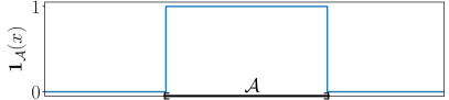
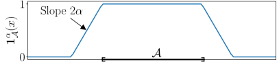
Figure 4: Illustration of the relaxation of the indicator function.

The parameter $\alpha$ quantifies the stiffness of the relaxation. As $\alpha\to+\infty$, the relaxed indicator $\mathbf{1}_{\mathcal{A}}^{\alpha}$ converges pointwise towards the original indicator function $\mathbf{1}_{\mathcal{A}}$. As $\alpha\to 0$, the relaxed indicator $\mathbf{1}_{\mathcal{A}}^{\alpha}$ converges pointwise towards the constant function $1$. Note that for all $\alpha>0$, the relaxed indicator $\mathbf{1}_{\mathcal{A}}^{\alpha}$ is continuous and differentiable almost everywhere.

A continuous relaxation of the system dynamics of parameter $\alpha$ is obtained by replacing the occurrences of the indicator function by its relaxed version. For instance, the relaxed dynamics of the stock is obtained from (2.20):

$$\boldsymbol{S^{\textstyle\text{\unboldmath$\scriptstyle$}}_{\textstyle\text{\unboldmath$\scriptstyle t+1$}}}=\boldsymbol{S^{\textstyle\text{\unboldmath$\scriptstyle$}}_{\textstyle\text{\unboldmath$\scriptstyle t$}}}+\sum_{i=1}^{n}\sum_{d=1}^{D}\mathbf{1}_{\{D-1\}}^{\alpha}(\boldsymbol{P^{\textstyle\text{\unboldmath$\scriptstyle d$}}_{\textstyle\text{\unboldmath$\scriptstyle i,t$}}})-\min\Big{(}\boldsymbol{S^{\textstyle\text{\unboldmath$\scriptstyle$}}_{\textstyle\text{\unboldmath$\scriptstyle t$}}},\ \sum_{i=1}^{n}\mathbf{1}_{\{0\}}^{\alpha}(\boldsymbol{E^{\textstyle\text{\unboldmath$\scriptstyle$}}_{\textstyle\text{\unboldmath$\scriptstyle i,t$}}})\Big{)}\;.$$ (4.10)

Additional technical details and an explicit expression for the relaxed dynamics of the components are given in Appendix B. The relaxed dynamics and relaxed auxiliary dynamics are denoted by $\Theta^{\alpha}$ and $\Phi^{\alpha}$ respectively.

4.3.3 Cost relaxation

The relaxation of the maintenance cost and forced outage cost is constructed using the same technique as for the dynamics. Let $i\in\mathbb{I}$, $t\in\mathbb{T}$ and $\alpha>0$ be given.

• The relaxed maintenance cost for component $i$ at time $t$ with parameter $\alpha$ is defined as:

  $$\left\{\begin{aligned} j^{\alpha}_{i,t}(\boldsymbol{X^{\textstyle\text{\unboldmath$\scriptstyle$}}_{\textstyle\text{\unboldmath$\scriptstyle i,t$}}},u_{i,t})&=\eta_{t}C^{P}_{i}u_{i,t}^{2}+\eta_{t}C^{C}_{i}\mathbf{1}_{\{0\}}^{\alpha}(\boldsymbol{E^{\textstyle\text{\unboldmath$\scriptstyle$}}_{\textstyle\text{\unboldmath$\scriptstyle i,t$}}})\mathbf{1}_{\{0\}}^{\alpha}(\boldsymbol{A^{\textstyle\text{\unboldmath$\scriptstyle$}}_{\textstyle\text{\unboldmath$\scriptstyle i,t$}}}),\quad t\in\mathbb{T}_{-1}\;,\\ j^{\alpha}_{i,T}(\boldsymbol{X^{\textstyle\text{\unboldmath$\scriptstyle$}}_{\textstyle\text{\unboldmath$\scriptstyle i,T$}}})&=\eta_{T}C^{C}_{i}\mathbf{1}_{\{0\}}^{\alpha}(\boldsymbol{E^{\textstyle\text{\unboldmath$\scriptstyle$}}_{\textstyle\text{\unboldmath$\scriptstyle i,T$}}})\mathbf{1}_{\{0\}}^{\alpha}(\boldsymbol{A^{\textstyle\text{\unboldmath$\scriptstyle$}}_{\textstyle\text{\unboldmath$\scriptstyle i,T$}}})\;.\end{aligned}\right.$$ (4.11)

• The relaxed forced outage cost at time $t$ with parameter $\alpha$ is defined as:

  $$j^{F,\alpha}_{t}(\boldsymbol{X^{\textstyle\text{\unboldmath$\scriptstyle$}}_{\textstyle\text{\unboldmath$\scriptstyle 1:n,t$}}})=\eta_{t}C^{F}\min\left\{1,\ \sum_{i=1}^{n}\mathbf{1}_{\{0\}}^{\alpha}(\boldsymbol{E^{\textstyle\text{\unboldmath$\scriptstyle$}}_{\textstyle\text{\unboldmath$\scriptstyle i,t$}}})\mathbf{1}_{\mathbb{R}_{+}^{*}}^{\alpha}(\boldsymbol{A^{\textstyle\text{\unboldmath$\scriptstyle$}}_{\textstyle\text{\unboldmath$\scriptstyle i,t$}}})\right\}\;.$$ (4.12)

Similarly, as in (2.25) and (2.26), we set:

$$j^{\alpha}_{i}(\boldsymbol{X^{\textstyle\text{\unboldmath$\scriptstyle$}}_{\textstyle\text{\unboldmath$\scriptstyle i$}}},u_{i})=\sum_{t=0}^{T-1}j^{\alpha}_{i,t}(\boldsymbol{X^{\textstyle\text{\unboldmath$\scriptstyle$}}_{\textstyle\text{\unboldmath$\scriptstyle i,t$}}},u_{i,t})+j^{\alpha}_{i,T}(\boldsymbol{X^{\textstyle\text{\unboldmath$\scriptstyle$}}_{\textstyle\text{\unboldmath$\scriptstyle i,T$}}})\quad\text{and}\quad j^{F,\alpha}(\boldsymbol{X^{\textstyle\text{\unboldmath$\scriptstyle$}}_{\textstyle\text{\unboldmath$\scriptstyle 1:n$}}})=\sum_{t=0}^{T}j^{F,\alpha}_{t}(\boldsymbol{X^{\textstyle\text{\unboldmath$\scriptstyle$}}_{\textstyle\text{\unboldmath$\scriptstyle 1:n,t$}}})\;.$$ (4.13)

We use the relaxed version of the dynamics $\Theta^{\alpha}$, of the auxiliary dynamics $\Phi^{\alpha}$, and of the costs $j^{\alpha}_{i}$ and $j^{F,\alpha}$ in the auxiliary problem (4.8). Hence, the objective function and the dynamics are continuous and differentiable almost everywhere with respect to $(\boldsymbol{X^{\textstyle\text{\unboldmath$\scriptstyle$}}_{\textstyle\text{\unboldmath$\scriptstyle$}}},\boldsymbol{S^{\textstyle\text{\unboldmath$\scriptstyle$}}_{\textstyle\text{\unboldmath$\scriptstyle$}}},u)$. Note that the choice of the relaxation parameter $\alpha$ plays an important role. We can guess that choosing a low value for $\alpha$ leads to a problem that may be easier to solve numerically than with a larger value of $\alpha$. However, with a low value of $\alpha$ the relaxed dynamics and cost do not represent well the industrial problem whereas with a large $\alpha$ the original and relaxed dynamics are close. More details on the influence of the parameter $\alpha$ and how it is chosen in practice are given in §5.1.

4.4 Explicit expression of the subproblems

By construction, the auxiliary problem (4.8) can be decomposed into $n$ independent subproblems on the components and a subproblem on the stock. In this section, we provide the explicit expression of these subproblems. The APP fixed-point algorithm will be applied on the relaxed system, so we use the relaxed dynamics and cost in the writing of the subproblems. Formally, the gradients of $\Theta^{\alpha}$ and $\Phi^{\alpha}$ are not defined everywhere. By abuse of notation, the subproblems are given as if $\Theta^{\alpha}$ and $\Phi^{\alpha}$ were differentiable. Appendix D gives details on how we handle the points where the relaxed indicator is not differentiable.

The subproblem on component $i\in\mathbb{I}$ is:

$$\min_{(\boldsymbol{X^{\textstyle\text{\unboldmath$\scriptstyle$}}_{\textstyle\text{\unboldmath$\scriptstyle i$}}},u_{i})\in\mathcal{X}_{i}\times\mathbb{U}_{i}} \ \begin{multlined}\mathbb{E}\bigg{(}j^{\alpha}_{i}(\boldsymbol{X^{\textstyle\text{\unboldmath$\scriptstyle$}}_{\textstyle\text{\unboldmath$\scriptstyle i$}}},u_{i})+j^{F,\alpha}(\bar{\boldsymbol{X^{\textstyle\text{\unboldmath$\scriptstyle$}}_{\textstyle\text{\unboldmath$\scriptstyle$}}}}_{1:i-1},\boldsymbol{X^{\textstyle\text{\unboldmath$\scriptstyle$}}_{\textstyle\text{\unboldmath$\scriptstyle i$}}},\bar{\boldsymbol{X^{\textstyle\text{\unboldmath$\scriptstyle$}}_{\textstyle\text{\unboldmath$\scriptstyle$}}}}_{i+1:n})\\ +\frac{\gamma_{x}}{2}\left\|\boldsymbol{X^{\textstyle\text{\unboldmath$\scriptstyle$}}_{\textstyle\text{\unboldmath$\scriptstyle i$}}}-\bar{\boldsymbol{X^{\textstyle\text{\unboldmath$\scriptstyle$}}_{\textstyle\text{\unboldmath$\scriptstyle$}}}}_{i}\right\|^{2}+\frac{\gamma_{u}}{2}\left\|u_{i}-\bar{u}_{i}\right\|^{2}\\ +\left\langle\bar{\boldsymbol{\Lambda^{\textstyle\text{\unboldmath$\scriptstyle$}}_{\textstyle\text{\unboldmath$\scriptstyle$}}}}_{\boldsymbol{S^{\textstyle\text{\unboldmath$\scriptstyle$}}_{\textstyle\text{\unboldmath$\scriptstyle$}}}}\>,\partial_{\boldsymbol{X^{\textstyle\text{\unboldmath$\scriptstyle$}}_{\textstyle\text{\unboldmath$\scriptstyle i$}}}}\Theta_{\boldsymbol{S^{\textstyle\text{\unboldmath$\scriptstyle$}}_{\textstyle\text{\unboldmath$\scriptstyle$}}}}^{\alpha}(\bar{\boldsymbol{X^{\textstyle\text{\unboldmath$\scriptstyle$}}_{\textstyle\text{\unboldmath$\scriptstyle$}}}}_{1:n},\bar{\boldsymbol{S^{\textstyle\text{\unboldmath$\scriptstyle$}}_{\textstyle\text{\unboldmath$\scriptstyle$}}}})\cdot\boldsymbol{X^{\textstyle\text{\unboldmath$\scriptstyle$}}_{\textstyle\text{\unboldmath$\scriptstyle i$}}}\right\rangle\\ +\sum_{j=i+1}^{n}\left\langle\bar{\boldsymbol{\Lambda^{\textstyle\text{\unboldmath$\scriptstyle$}}_{\textstyle\text{\unboldmath$\scriptstyle$}}}}_{j}\>,\partial_{\boldsymbol{X^{\textstyle\text{\unboldmath$\scriptstyle$}}_{\textstyle\text{\unboldmath$\scriptstyle i$}}}}\Theta_{j}^{\alpha}(\bar{\boldsymbol{X^{\textstyle\text{\unboldmath$\scriptstyle$}}_{\textstyle\text{\unboldmath$\scriptstyle$}}}}_{1:j},\bar{\boldsymbol{S^{\textstyle\text{\unboldmath$\scriptstyle$}}_{\textstyle\text{\unboldmath$\scriptstyle$}}}},\bar{u}_{j},\boldsymbol{W^{\textstyle\text{\unboldmath$\scriptstyle$}}_{\textstyle\text{\unboldmath$\scriptstyle j$}}})\cdot\boldsymbol{X^{\textstyle\text{\unboldmath$\scriptstyle$}}_{\textstyle\text{\unboldmath$\scriptstyle i$}}}\right\rangle\bigg{)}\end{multlined}\mathbb{E}\bigg{(}j^{\alpha}_{i}(\boldsymbol{X^{\textstyle\text{\unboldmath$\scriptstyle$}}_{\textstyle\text{\unboldmath$\scriptstyle i$}}},u_{i})+j^{F,\alpha}(\bar{\boldsymbol{X^{\textstyle\text{\unboldmath$\scriptstyle$}}_{\textstyle\text{\unboldmath$\scriptstyle$}}}}_{1:i-1},\boldsymbol{X^{\textstyle\text{\unboldmath$\scriptstyle$}}_{\textstyle\text{\unboldmath$\scriptstyle i$}}},\bar{\boldsymbol{X^{\textstyle\text{\unboldmath$\scriptstyle$}}_{\textstyle\text{\unboldmath$\scriptstyle$}}}}_{i+1:n})\\ +\frac{\gamma_{x}}{2}\left\|\boldsymbol{X^{\textstyle\text{\unboldmath$\scriptstyle$}}_{\textstyle\text{\unboldmath$\scriptstyle i$}}}-\bar{\boldsymbol{X^{\textstyle\text{\unboldmath$\scriptstyle$}}_{\textstyle\text{\unboldmath$\scriptstyle$}}}}_{i}\right\|^{2}+\frac{\gamma_{u}}{2}\left\|u_{i}-\bar{u}_{i}\right\|^{2}\\ +\left\langle\bar{\boldsymbol{\Lambda^{\textstyle\text{\unboldmath$\scriptstyle$}}_{\textstyle\text{\unboldmath$\scriptstyle$}}}}_{\boldsymbol{S^{\textstyle\text{\unboldmath$\scriptstyle$}}_{\textstyle\text{\unboldmath$\scriptstyle$}}}}\>,\partial_{\boldsymbol{X^{\textstyle\text{\unboldmath$\scriptstyle$}}_{\textstyle\text{\unboldmath$\scriptstyle i$}}}}\Theta_{\boldsymbol{S^{\textstyle\text{\unboldmath$\scriptstyle$}}_{\textstyle\text{\unboldmath$\scriptstyle$}}}}^{\alpha}(\bar{\boldsymbol{X^{\textstyle\text{\unboldmath$\scriptstyle$}}_{\textstyle\text{\unboldmath$\scriptstyle$}}}}_{1:n},\bar{\boldsymbol{S^{\textstyle\text{\unboldmath$\scriptstyle$}}_{\textstyle\text{\unboldmath$\scriptstyle$}}}})\cdot\boldsymbol{X^{\textstyle\text{\unboldmath$\scriptstyle$}}_{\textstyle\text{\unboldmath$\scriptstyle i$}}}\right\rangle\\ +\sum_{j=i+1}^{n}\left\langle\bar{\boldsymbol{\Lambda^{\textstyle\text{\unboldmath$\scriptstyle$}}_{\textstyle\text{\unboldmath$\scriptstyle$}}}}_{j}\>,\partial_{\boldsymbol{X^{\textstyle\text{\unboldmath$\scriptstyle$}}_{\textstyle\text{\unboldmath$\scriptstyle i$}}}}\Theta_{j}^{\alpha}(\bar{\boldsymbol{X^{\textstyle\text{\unboldmath$\scriptstyle$}}_{\textstyle\text{\unboldmath$\scriptstyle$}}}}_{1:j},\bar{\boldsymbol{S^{\textstyle\text{\unboldmath$\scriptstyle$}}_{\textstyle\text{\unboldmath$\scriptstyle$}}}},\bar{u}_{j},\boldsymbol{W^{\textstyle\text{\unboldmath$\scriptstyle$}}_{\textstyle\text{\unboldmath$\scriptstyle j$}}})\cdot\boldsymbol{X^{\textstyle\text{\unboldmath$\scriptstyle$}}_{\textstyle\text{\unboldmath$\scriptstyle i$}}}\right\rangle\bigg{)}$$ (4.14)

$$\mathrm{s.t.} \ \Phi_{i}^{\alpha}(\boldsymbol{X^{\textstyle\text{\unboldmath$\scriptstyle$}}_{\textstyle\text{\unboldmath$\scriptstyle i$}}},u_{i},\boldsymbol{W^{\textstyle\text{\unboldmath$\scriptstyle$}}_{\textstyle\text{\unboldmath$\scriptstyle i$}}})=0\;.$$

The subproblem on the stock is:

$$\min_{\boldsymbol{S^{\textstyle\text{\unboldmath$\scriptstyle$}}_{\textstyle\text{\unboldmath$\scriptstyle$}}}\in\mathcal{S}} \ \mathbb{E}\left(\frac{\gamma_{s}}{2}\left\|\boldsymbol{S^{\textstyle\text{\unboldmath$\scriptstyle$}}_{\textstyle\text{\unboldmath$\scriptstyle$}}}-\bar{\boldsymbol{S^{\textstyle\text{\unboldmath$\scriptstyle$}}_{\textstyle\text{\unboldmath$\scriptstyle$}}}}\right\|^{2}+\sum_{i=1}^{n}\left\langle\bar{\boldsymbol{\Lambda^{\textstyle\text{\unboldmath$\scriptstyle$}}_{\textstyle\text{\unboldmath$\scriptstyle$}}}}_{i}\>,\partial_{\boldsymbol{S^{\textstyle\text{\unboldmath$\scriptstyle$}}_{\textstyle\text{\unboldmath$\scriptstyle$}}}}\Theta_{i}^{\alpha}(\bar{\boldsymbol{X^{\textstyle\text{\unboldmath$\scriptstyle$}}_{\textstyle\text{\unboldmath$\scriptstyle$}}}}_{1:i},\bar{\boldsymbol{S^{\textstyle\text{\unboldmath$\scriptstyle$}}_{\textstyle\text{\unboldmath$\scriptstyle$}}}},\bar{u}_{i},\boldsymbol{W^{\textstyle\text{\unboldmath$\scriptstyle$}}_{\textstyle\text{\unboldmath$\scriptstyle i$}}})\cdot\boldsymbol{S^{\textstyle\text{\unboldmath$\scriptstyle$}}_{\textstyle\text{\unboldmath$\scriptstyle$}}}\right\rangle\right)$$ (4.15)

$$\mathrm{s.t.} \ \Phi_{\boldsymbol{S^{\textstyle\text{\unboldmath$\scriptstyle$}}_{\textstyle\text{\unboldmath$\scriptstyle$}}}}^{\alpha}(\boldsymbol{S^{\textstyle\text{\unboldmath$\scriptstyle$}}_{\textstyle\text{\unboldmath$\scriptstyle$}}})=0\;.$$

4.5 The APP fixed-point algorithm for the industrial system

We can now solve the original maintenance optimization problem (2.27) using the fixed-point algorithm 1. In this section, we give details on the practical implementation of the algorithm and present an efficient mixed parallel and sequential strategy for the resolution of the subproblems, that is tailored for the industrial optimization problem.

At each iteration, we solve the auxiliary problem (4.8). In a fully parallel version of the APP fixed-point algorithm, solving the auxiliary problem (4.8) boils down to the parallel resolution of the $n+1$ independent subproblems defined by (4.14)–(4.15).

1. The subproblems on the components (4.14) are solved with the blackbox algorithm MADS [7]. At iteration $k$, we solve subproblem $i\in\mathbb{I}$ with:

   $$(\bar{\boldsymbol{X^{\textstyle\text{\unboldmath$\scriptstyle$}}_{\textstyle\text{\unboldmath$\scriptstyle$}}}},\bar{\boldsymbol{S^{\textstyle\text{\unboldmath$\scriptstyle$}}_{\textstyle\text{\unboldmath$\scriptstyle$}}}},\bar{u})=(\boldsymbol{X^{\textstyle\text{\unboldmath$\scriptstyle k$}}_{\textstyle\text{\unboldmath$\scriptstyle$}}},\boldsymbol{S^{\textstyle\text{\unboldmath$\scriptstyle k$}}_{\textstyle\text{\unboldmath$\scriptstyle$}}},u^{k})\quad\text{and}\quad\bar{\boldsymbol{\Lambda^{\textstyle\text{\unboldmath$\scriptstyle$}}_{\textstyle\text{\unboldmath$\scriptstyle$}}}}=\boldsymbol{\Lambda^{\textstyle\text{\unboldmath$\scriptstyle k$}}_{\textstyle\text{\unboldmath$\scriptstyle$}}}\;.$$ (4.16)

   MADS outputs a primal solution $(\boldsymbol{X^{\textstyle\text{\unboldmath$\scriptstyle k+1$}}_{\textstyle\text{\unboldmath$\scriptstyle i$}}},u_{i}^{k+1})$. The optimal multiplier $\boldsymbol{\Lambda^{\textstyle\text{\unboldmath$\scriptstyle k+1$}}_{\textstyle\text{\unboldmath$\scriptstyle i$}}}$ is computed afterwards using the adjoint state. The full derivation of the backward recursion for the multipliers in the industrial case is carried out in Appendix C.

2. The subproblem on the stock (4.15) is very easy to solve numerically. At iteration $k$ of the fully parallel APP fixed-point algorithm, we use:

   $$(\bar{\boldsymbol{X^{\textstyle\text{\unboldmath$\scriptstyle$}}_{\textstyle\text{\unboldmath$\scriptstyle$}}}},\bar{\boldsymbol{S^{\textstyle\text{\unboldmath$\scriptstyle$}}_{\textstyle\text{\unboldmath$\scriptstyle$}}}},\bar{u})=(\boldsymbol{X^{\textstyle\text{\unboldmath$\scriptstyle k$}}_{\textstyle\text{\unboldmath$\scriptstyle$}}},\boldsymbol{S^{\textstyle\text{\unboldmath$\scriptstyle k$}}_{\textstyle\text{\unboldmath$\scriptstyle$}}},u^{k})\quad\text{and}\quad\bar{\boldsymbol{\Lambda^{\textstyle\text{\unboldmath$\scriptstyle$}}_{\textstyle\text{\unboldmath$\scriptstyle$}}}}=\boldsymbol{\Lambda^{\textstyle\text{\unboldmath$\scriptstyle k$}}_{\textstyle\text{\unboldmath$\scriptstyle$}}}\;.$$ (4.17)

   The constraint $\Phi_{\boldsymbol{S^{\textstyle\text{\unboldmath$\scriptstyle$}}_{\textstyle\text{\unboldmath$\scriptstyle$}}}}^{\alpha}(\boldsymbol{S^{\textstyle\text{\unboldmath$\scriptstyle$}}_{\textstyle\text{\unboldmath$\scriptstyle$}}})=0$ represents the dynamics of the stock with $\bar{\boldsymbol{X^{\textstyle\text{\unboldmath$\scriptstyle$}}_{\textstyle\text{\unboldmath$\scriptstyle$}}}}=\boldsymbol{X^{\textstyle\text{\unboldmath$\scriptstyle k$}}_{\textstyle\text{\unboldmath$\scriptstyle$}}}$ being fixed. The value of $\bar{\boldsymbol{X^{\textstyle\text{\unboldmath$\scriptstyle$}}_{\textstyle\text{\unboldmath$\scriptstyle$}}}}$ completely determines the dynamics of the stock. Hence, solving the subproblem on the stock just boils down to simulate its dynamics, we get a primal solution $\boldsymbol{S^{\textstyle\text{\unboldmath$\scriptstyle k+1$}}_{\textstyle\text{\unboldmath$\scriptstyle$}}}$. The optimal multiplier $\boldsymbol{\Lambda^{\textstyle\text{\unboldmath$\scriptstyle k+1$}}_{\textstyle\text{\unboldmath$\scriptstyle\boldsymbol{S^{\textstyle\text{\unboldmath$\scriptstyle$}}_{\textstyle\text{\unboldmath$\scriptstyle$}}}$}}}$ is also computed using the adjoint state, see Appendix C.

The features of the subproblem on the stock suggest to change the fully parallel strategy into a mixed parallel/sequential strategy.

1. At iteration $k$, the $n$ subproblems on the components are still solved in parallel using:

   $$(\bar{\boldsymbol{X^{\textstyle\text{\unboldmath$\scriptstyle$}}_{\textstyle\text{\unboldmath$\scriptstyle$}}}},\bar{\boldsymbol{S^{\textstyle\text{\unboldmath$\scriptstyle$}}_{\textstyle\text{\unboldmath$\scriptstyle$}}}},\bar{u})=(\boldsymbol{X^{\textstyle\text{\unboldmath$\scriptstyle k$}}_{\textstyle\text{\unboldmath$\scriptstyle$}}},\boldsymbol{S^{\textstyle\text{\unboldmath$\scriptstyle k$}}_{\textstyle\text{\unboldmath$\scriptstyle$}}},u^{k})\quad\text{and}\quad\bar{\boldsymbol{\Lambda^{\textstyle\text{\unboldmath$\scriptstyle$}}_{\textstyle\text{\unboldmath$\scriptstyle$}}}}=\boldsymbol{\Lambda^{\textstyle\text{\unboldmath$\scriptstyle k$}}_{\textstyle\text{\unboldmath$\scriptstyle$}}}\;.$$ (4.18)

   This yields a solution $(\boldsymbol{X^{\textstyle\text{\unboldmath$\scriptstyle k+1$}}_{\textstyle\text{\unboldmath$\scriptstyle i$}}},u_{i}^{k+1},\boldsymbol{\Lambda^{\textstyle\text{\unboldmath$\scriptstyle k+1$}}_{\textstyle\text{\unboldmath$\scriptstyle i$}}})$ for each subproblem $i\in\mathbb{I}$.

2. The difference arises for the subproblem on the stock. At iteration $k$, we immediately use the output of the subproblems on the components. This means that we set before solving the subproblem on the stock at iteration $k$:

   $$(\bar{\boldsymbol{X^{\textstyle\text{\unboldmath$\scriptstyle$}}_{\textstyle\text{\unboldmath$\scriptstyle$}}}},\bar{u})=(\boldsymbol{X^{\textstyle\text{\unboldmath$\scriptstyle k+1$}}_{\textstyle\text{\unboldmath$\scriptstyle$}}},u^{k+1})\quad\text{and}\quad(\bar{\boldsymbol{\Lambda^{\textstyle\text{\unboldmath$\scriptstyle$}}_{\textstyle\text{\unboldmath$\scriptstyle$}}}}_{1},\ldots,\bar{\boldsymbol{\Lambda^{\textstyle\text{\unboldmath$\scriptstyle$}}_{\textstyle\text{\unboldmath$\scriptstyle$}}}}_{n}) =(\boldsymbol{\Lambda^{\textstyle\text{\unboldmath$\scriptstyle k+1$}}_{\textstyle\text{\unboldmath$\scriptstyle 1$}}},\ldots,\boldsymbol{\Lambda^{\textstyle\text{\unboldmath$\scriptstyle k+1$}}_{\textstyle\text{\unboldmath$\scriptstyle n$}}})\;.$$ (4.19)

   This implies that the subproblem on the stock at iteration $k$ can be solved only after all subproblems on the components have been solved.

With this strategy, we see experimentally that the number of iterations for convergence is reduced without penalizing the computation time per iteration as the subproblem on the stock can be solved in negligible time. This results in an overall speed up of the algorithm. The APP fixed-point algorithm with the mixed parallel/sequential strategy is presented in Algorithm 2. The termination criterion is a maximum number of iterations $M\in\mathbb{N}$. This is the version that is used for the numerical experiments.

1:0Start with $(\bar{\boldsymbol{X^{\textstyle\text{\unboldmath$\scriptstyle$}}_{\textstyle\text{\unboldmath$\scriptstyle$}}}},\bar{\boldsymbol{S^{\textstyle\text{\unboldmath$\scriptstyle$}}_{\textstyle\text{\unboldmath$\scriptstyle$}}}},\bar{u})=(\boldsymbol{X^{\textstyle\text{\unboldmath$\scriptstyle 0$}}_{\textstyle\text{\unboldmath$\scriptstyle$}}},\boldsymbol{S^{\textstyle\text{\unboldmath$\scriptstyle 0$}}_{\textstyle\text{\unboldmath$\scriptstyle$}}},u^{0})$, $\bar{\boldsymbol{\Lambda^{\textstyle\text{\unboldmath$\scriptstyle$}}_{\textstyle\text{\unboldmath$\scriptstyle$}}}}=\boldsymbol{\Lambda^{\textstyle\text{\unboldmath$\scriptstyle 0$}}_{\textstyle\text{\unboldmath$\scriptstyle$}}}$

2:-1$k=0,\ldots,M-1$

3:-2$i\in\{1,\ldots,n\}$

4:-3Solve the subproblem (4.14) on component $i$.

5:-4Let $(\boldsymbol{X^{\textstyle\text{\unboldmath$\scriptstyle k+1$}}_{\textstyle\text{\unboldmath$\scriptstyle i$}}},u_{i}^{k+1})$ be a solution and $\boldsymbol{\Lambda^{\textstyle\text{\unboldmath$\scriptstyle k+1$}}_{\textstyle\text{\unboldmath$\scriptstyle i$}}}$ be an optimal multiplier.

6:-5

7:-6Set $(\bar{\boldsymbol{X^{\textstyle\text{\unboldmath$\scriptstyle$}}_{\textstyle\text{\unboldmath$\scriptstyle$}}}},\bar{u})=((\boldsymbol{X^{\textstyle\text{\unboldmath$\scriptstyle k+1$}}_{\textstyle\text{\unboldmath$\scriptstyle 1$}}},\ldots,\boldsymbol{X^{\textstyle\text{\unboldmath$\scriptstyle k+1$}}_{\textstyle\text{\unboldmath$\scriptstyle n$}}}),(u_{1}^{k+1},\ldots,u_{n}^{k+1}))$

8:-7Set $(\bar{\boldsymbol{\Lambda^{\textstyle\text{\unboldmath$\scriptstyle$}}_{\textstyle\text{\unboldmath$\scriptstyle$}}}}_{1},\ldots,\bar{\boldsymbol{\Lambda^{\textstyle\text{\unboldmath$\scriptstyle$}}_{\textstyle\text{\unboldmath$\scriptstyle$}}}}_{n})=(\boldsymbol{\Lambda^{\textstyle\text{\unboldmath$\scriptstyle k+1$}}_{\textstyle\text{\unboldmath$\scriptstyle 1$}}},\ldots,\boldsymbol{\Lambda^{\textstyle\text{\unboldmath$\scriptstyle k+1$}}_{\textstyle\text{\unboldmath$\scriptstyle n$}}})$

9:-8Solve the subproblem (4.15) on the stock.

10:-9Let $\boldsymbol{S^{\textstyle\text{\unboldmath$\scriptstyle k+1$}}_{\textstyle\text{\unboldmath$\scriptstyle$}}}$ be a solution and $\boldsymbol{\Lambda^{\textstyle\text{\unboldmath$\scriptstyle k+1$}}_{\textstyle\text{\unboldmath$\scriptstyle\boldsymbol{S^{\textstyle\text{\unboldmath$\scriptstyle$}}_{\textstyle\text{\unboldmath$\scriptstyle$}}}$}}}$ be an optimal multiplier.

11:-10Set $\bar{\boldsymbol{S^{\textstyle\text{\unboldmath$\scriptstyle$}}_{\textstyle\text{\unboldmath$\scriptstyle$}}}}=\boldsymbol{S^{\textstyle\text{\unboldmath$\scriptstyle k+1$}}_{\textstyle\text{\unboldmath$\scriptstyle$}}}$ and $\bar{\boldsymbol{\Lambda^{\textstyle\text{\unboldmath$\scriptstyle$}}_{\textstyle\text{\unboldmath$\scriptstyle$}}}}_{\boldsymbol{S^{\textstyle\text{\unboldmath$\scriptstyle$}}_{\textstyle\text{\unboldmath$\scriptstyle$}}}}=\boldsymbol{\Lambda^{\textstyle\text{\unboldmath$\scriptstyle k+1$}}_{\textstyle\text{\unboldmath$\scriptstyle\boldsymbol{S^{\textstyle\text{\unboldmath$\scriptstyle$}}_{\textstyle\text{\unboldmath$\scriptstyle$}}}$}}}$

12:-11

13:-12return the maintenance strategy $u^{M}$

Algorithm 2 APP fixed-point algorithm with a mixed parallel/sequential strategy

5 Numerical results

In this part, we present the results of the decomposition methodology applied to Problem (2.27). The expectation in (2.27) cannot be evaluated exactly, so we solve a Monte-Carlo approximation of the problem with $Q$ fixed failure scenarios $\omega_{1},\ldots,\omega_{Q}\in\Omega$:

$$\min_{(\boldsymbol{X^{\textstyle\text{\unboldmath$\scriptstyle$}}_{\textstyle\text{\unboldmath$\scriptstyle$}}},\boldsymbol{S^{\textstyle\text{\unboldmath$\scriptstyle$}}_{\textstyle\text{\unboldmath$\scriptstyle$}}},u)\in\mathcal{X}\times\mathcal{S}\times\mathbb{U}} \frac{1}{Q}\sum_{q=1}^{Q}\left(\sum_{i=1}^{n}j_{i}\left(\boldsymbol{X^{\textstyle\text{\unboldmath$\scriptstyle$}}_{\textstyle\text{\unboldmath$\scriptstyle i$}}}(\omega_{q}\right),u_{i})+j^{F}\left(\boldsymbol{X^{\textstyle\text{\unboldmath$\scriptstyle$}}_{\textstyle\text{\unboldmath$\scriptstyle 1:n$}}}(\omega_{q})\right)\right)$$ (5.1)

$$\mathrm{s.t.} \Theta\left(\boldsymbol{X^{\textstyle\text{\unboldmath$\scriptstyle$}}_{\textstyle\text{\unboldmath$\scriptstyle$}}}(\omega_{q}),\boldsymbol{S^{\textstyle\text{\unboldmath$\scriptstyle$}}_{\textstyle\text{\unboldmath$\scriptstyle$}}}(\omega_{q}),u,\boldsymbol{W^{\textstyle\text{\unboldmath$\scriptstyle$}}_{\textstyle\text{\unboldmath$\scriptstyle$}}}(\omega_{q})\right)=0,\quad q\in\{1,\ldots,Q\}\;.$$

The aim of this work is to show that the decomposition by prediction can efficiently solve a maintenance problem with a large number of components. We consider two test cases with the characteristics given in Table 1. As a maintenance strategy is parametrized by the vector $u\in\mathbb{U}$ given in (2.8), the optimization problem for the $80$-component case involves $nT=80\times 40=3200$ variables.

The synthetic systems described in Table 1 do not exactly represent a real situation but are meant to be a proxy for the real cases presented at the beginning of §2.1:

1. The situation where we consider turbines of the same production unit is simpler than the synthetic systems as it has fewer components (up to $10$ for the real case and $80$ in the synthetic case).

2. On the other hand, the situation where we consider turbines across several production units is slightly more complicated than the synthetic systems: in our model all components belong to the same unit, therefore the forced outage cost is simpler than in reality. However, the decomposition methodology can be applied to this real case exactly as for the synthetic cases.

3. For the case of a system with several families of components with a stock of spare parts for each family, the decomposition methodology is still applicable and will result in an additional subproblem for each stock. However, we have seen in §4.5 that these subproblems are solved in negligible time as they just amount to the simulation of the dynamics of the corresponding stock. Hence, these additional subproblems do not slow down the method compared to the synthetic cases. The expression of the forced outage cost may also be slightly more complicated than for the synthetic cases.

The costs and the failure distributions used in Table 1 are of the same order of magnitude as what is encountered in practice. In the first test case, the failure distributions are chosen so that the mean time to failure of the components is in the lower limit of the real cases, which induces a large number of failures in the system. This is the situation where the PM strategy has the most significant influence on the economic performance of the system. In the second test case, we consider components with a longer lifespan but the stock has fewer parts than in the first case. This induces a strong coupling between the stock and the components. These cases can be considered to be stress tests for the optimization algorithms.

Parameter	Case 1	Case 2
Number of components $n$	$80$	$80$
Initial number of spare parts $\boldsymbol{S^{\textstyle\text{\unboldmath$\scriptstyle$}}_{\textstyle\text{\unboldmath$\scriptstyle 0$}}}$	$\mathbf{16}$	$\mathbf{5}$
Horizon $T$	$40$ years	$40$ years
Time step $\Delta t$	$1$ year	$1$ year
Number of time steps for supply $D$	$2$	$2$
Discount rate $\tau$	$0.08$	$0.08$
Maintenance threshold $\nu$	$0.9$	$0.9$
Yearly forced outage cost $C^{F}$	$10000$ k€/ year	$10000$ k€/ year
Number of failure scenarios $Q$	$\mathbf{100}$	$\mathbf{300}$
Components characteristics
PM cost $C^{P}$	$50$ k€	$50$ k€
CM cost $C^{C}$	$200$ k€	$200$ k€
Failure distribution	$\mathbf{\mathrm{\textbf{Weib}}(3,10)}$	$\mathbf{\mathrm{\textbf{Weib}}(3,20)}$
Mean time to failure	$\mathbf{8.93}$ years	$\mathbf{17.86}$ years

Table 1: Characteristics of the test cases. Bold data represent the features that differ between the two cases.

5.1 Parameter tuning

Several parameters have to be tuned in order to apply the APP fixed-point algorithm. The parameters $\gamma_{x},\gamma_{s},\gamma_{u}$ appear in the auxiliary problem and $\alpha$ characterizes the relaxation of the system. These parameters are used in the APP fixed-point algorithm but not in the reference algorithm as the latter uses the original dynamics of the system to perform the optimization.

As the maintenance threshold $\nu$ is used both in the reference algorithm and the decomposition method, it is fixed to a value giving good performance with the reference algorithm. The same value of $\nu$ is used in the APP fixed-point algorithm. We do not consider changing the value of $\nu$ as it would mean that the reference algorithm changes for each different value of $\nu$, making a fair comparison harder and the results less clear to analyze.

5.1.1 Description of the parameters

In the auxiliary problem (4.8), the value of $\gamma=(\gamma_{x},\gamma_{s},\gamma_{u})$ influences the numerical behavior of the algorithm. We choose to increase the values of $\gamma_{x},\gamma_{s}$ and $\gamma_{u}$ at each iteration of the APP fixed-point algorithm. The insight is that we can use low values of $\gamma$ in the first iterations to get close to a good solution. Then, we use high values of $\gamma$ to avoid oscillations of the solution of the auxiliary problem. Indeed, with a large value of $\gamma$, the solution $(\boldsymbol{X^{\textstyle\text{\unboldmath$\scriptstyle k+1$}}_{\textstyle\text{\unboldmath$\scriptstyle$}}},\boldsymbol{S^{\textstyle\text{\unboldmath$\scriptstyle k+1$}}_{\textstyle\text{\unboldmath$\scriptstyle$}}},u^{k+1})$ of the auxiliary problem at iteration $k+1$ is close to the previous solution $(\boldsymbol{X^{\textstyle\text{\unboldmath$\scriptstyle k$}}_{\textstyle\text{\unboldmath$\scriptstyle$}}},\boldsymbol{S^{\textstyle\text{\unboldmath$\scriptstyle k$}}_{\textstyle\text{\unboldmath$\scriptstyle$}}},u^{k})$. The value of $\gamma_{u}$ evolves from iteration $k$ to $k+1$ of the APP fixed-point algorithm with an additive step $\Delta\gamma>0$, so that:

$$\gamma^{k+1}_{u}=\gamma^{k}_{u}+\Delta\gamma\;.$$ (5.2)

Then, $\gamma_{x}$ and $\gamma_{s}$ are chosen to be proportional to $\gamma_{u}$ with ratios $r_{x}>0$ and $r_{s}>0$ respectively, so that:

$$\gamma_{x}^{k+1}=\gamma_{u}^{k+1}/r_{x}\ \text{ and }\ \gamma_{s}^{k+1}=\gamma_{u}^{k+1}/r_{s}\;.$$ (5.3)

The motivation for this choice is that the vectors $\boldsymbol{X^{\textstyle\text{\unboldmath$\scriptstyle$}}_{\textstyle\text{\unboldmath$\scriptstyle$}}}$, $\boldsymbol{S^{\textstyle\text{\unboldmath$\scriptstyle$}}_{\textstyle\text{\unboldmath$\scriptstyle$}}}$ and $u$ need some rescaling so that their norms are of the same order of magnitude. The parameters $\gamma_{u}^{0},r_{x},r_{s},\Delta\gamma$ have to be tuned.

The other parameter that requires attention is the relaxation parameter $\alpha$. Similarly as for $\gamma$, we choose to increase the value of $\alpha$ at each iteration. A low value of $\alpha$ makes the problem easier to solve numerically but does not represent well the real problem. As $\alpha$ increases, the relaxed problem is closer and closer to the real one but becomes harder to solve. To ease the resolution, we use the solution of the auxiliary problem at iteration $k$ as a warm start in MADS for iteration $k+1$. The value of $\alpha$ varies from iteration $k$ to $k+1$ of the APP fixed-point algorithm with a step $\Delta\alpha>0$ so that:

$$\alpha^{k+1}=\alpha^{k}+\Delta\alpha\;.$$ (5.4)

The values of $\alpha^{0}$ and $\Delta\alpha$ have to be tuned. We denote by:

$$p=(\gamma_{u}^{0},r_{x},r_{s},\Delta\gamma,\alpha^{0},\Delta\alpha)\in\mathbb{R}^{6}\;,$$ (5.5)

the vector of parameters that have to be adjusted for the algorithm.

5.1.2 Tuning methodology

Choosing a good value for $p$ is difficult in practice. We cannot afford to test the fixed-point algorithm with many different values of $p$ directly on the $80$-component case, as one run of the optimization takes more than a day. In order to find an appropriate value for $p$, we rely on a smaller system than the $80$-component case. This small system is designed so that the runs of the fixed-point algorithm take a reasonable amount of time, $4$ hours in our case. The small system consists of $10$ components with $2$ spare parts initially. All the other characteristics of this small system are the same as Case 1 in Table 1. In a way, the $10$-component system can be seen as a downscaling of the $80$-component case of interest.

The idea of the tuning procedure is to run the decomposition method on the $10$-component system several times, but with a different value for $p$ at each run. To do so, we start by defining bounds on the value of the parameters, they are given in Table 2. These bounds are chosen to be wide in order to ensure that they contain good values of the parameters.

Parameter	$\gamma_{u}^{0}$	$r_{x}$	$r_{s}$	$\Delta\gamma$	$\alpha^{0}$	$\Delta\alpha$
Bounds	$[1,100]$	$[1,10^{4}]$	$[1,10^{3}]$	$[0,100]$	$[2,200]$	$[0,200]$

Table 2: Bounds for the parameters of the of the fixed-point algorithm.

Then, $200$ samples of $p$ are drawn with an optimized Latin Hypercube Sampling [15]. We run the fixed-point algorithm with each of the sampled values on the $10$-component system. The value of $p$ which gives the best result on the small system is used for the case with $80$ components. The chosen value is:

$$p=(17.32,\ 7434,\ 815.3,\ 1.360\times 10^{-1},\ 46.51,\ 135.5)\;.$$ (5.6)

We give the value of $p$ with $4$ significant digits to emphasize that the performance of the APP fixed-point algorithm is very sensitive to this value. A sensitivity analysis has been performed using a Morris method [9] but no clear pattern for a good choice of $p$ has been identified. More details on the methodology and results of the sensitivity analysis can be found in [8, §10.7].

5.2 Comparison of the decomposition method with MADS

Now that all the parameters of the fixed-point algorithm 2 are set, we can solve Problem (5.1). The performance of the fixed-point algorithm is compared with a reference algorithm, which is the blackbox algorithm MADS applied directly on Problem (5.1). We consider the systems of $80$ components described in Table 1. Parameters of the computation are given in Table 3. When running the optimization, the reference algorithm uses the original dynamics as it does not use gradient information. The APP fixed-point algorithm runs with the value of $p$ in (5.6) that parametrizes the auxiliary problem and the relaxation of the system.

	Decomposition	MADS
Fixed-point iterations	$50$	/
Cost function calls	$10^{3}$/subproblem/iteration	$10^{6}$
Cost and dynamics	Relaxed	Original
Processor model	Intel® Xeon® Processor E5-2680 v4, $2.4$ GHz

Table 3: Parameters of the computation for the two algorithms.

Remark 5.1.

The APP fixed-point algorithm solves a decomposable auxiliary problem at each iteration, this algorithm is designed to be parallelized. It runs on $80$ processors so that the subproblems on the components are solved in parallel. The reference algorithm MADS runs only on one processor. Note that it is also possible to parallelize MADS [6], although the implementation is not as straightforward as for the decomposition method. The parallel version of MADS has not been tested.

The maintenance strategies returned by the two algorithms are then evaluated on a common set of $10^{5}$ failure scenarios, distinct from those used for the optimization. For the two strategies, the evaluation is done with the original dynamics of the system in order to ensure a fair comparison. The two algorithms return a maintenance strategy with $u_{i,t}\in[0,1]$ for $(i,t)\in\mathbb{I}\times\mathbb{T}_{-1}$. From the operational perspective, PMs make the components as good as new. Hence, for the evaluation of the strategy, the controls are projected on $\{0,1\}$: we consider that if $u_{i,t}\geq\nu$, then the PM makes the component as good as new, otherwise no PM is performed. The comparison between the two maintenance strategies is fair as we use the same procedure for their evaluation.

5.2.1 Results for Case 1

The mean cost is $14509$ k€ with MADS and $12855$ k€ with the decomposition which represents a gain of $12\%$. The values of some quantiles are gathered in Table 4 and the distribution of the cost is represented on Fig. 6.

	$1\%$	$5\%$	$25\%$	$50\%$	$75\%$	$95\%$	$99\%$
Decomposition	$11641$	$11981$	$12469$	$12838$	$13221$	$13788$	$14182$
MADS	$13339$	$13663$	$14138$	$14494$	$14846$	$15406$	$15817$

Table 4: Quantiles of the cost of the two maintenance strategies (k€).

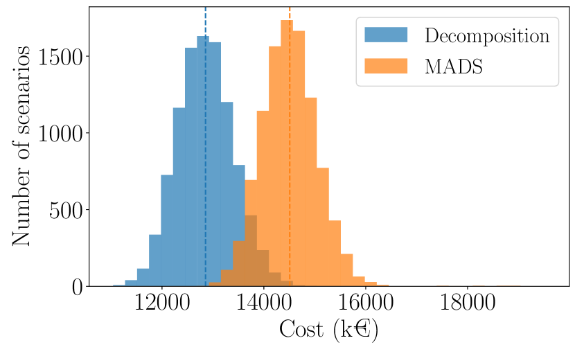
Figure 5: Distribution of the cost for the two maintenance strategies. The dashed lines represent the expected cost for both strategies.

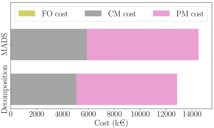
Figure 6: Part of the PM, CM and forced outage cost in the total expected cost.

Figure 6 outlines that both the CM cost and the PM cost are lower with the decomposition strategy. In fact the decomposition strategy performs more PMs than MADS strategy (Table 5) but these PMs occur later in time (Fig. 8). Because of the discount factor, the decomposition strategy is cheaper even if more PMs are performed. The forced outage cost is not visible on Fig. 6 as it represents $8.7$ k€ for MADS strategy and $2.7$ k€ for the decomposition strategy: there are very few scenarios where a forced outage occurs, again with an advantage for the decomposition strategy ($6$ occurrences in $10^{5}$ failure scenarios for the decomposition versus $36$ for MADS). Overall, the decomposition strategy performs PMs more effectively than MADS, both in terms of cost and in terms of number of failures and forced outages of the system.

Table 5 also provides the computation time for both methods. As we design a long term maintenance schedule, the focus is on the performance of the maintenance strategy and not on the running time of the methods that are acceptable for our purpose. The parameters of the algorithms have been tuned to allow similar numbers of function calls for both methods. The decomposition is slower as it uses the relaxed dynamics which is slower to compute than the original dynamics used by MADS.

	Decomposition	MADS
Total number of PMs	$669$	$595$
Mean number of PMs / component	$8.4$	$7.4$
Mean number of failures / component	$1.18$	$1.48$
Number of forced outages / Number of scenarios	$6/10000$	$36/10000$
Computation time	$2$ days, $1$ hour	$1$ day, $7$ hours

Table 5: Number of PMs, failures and forced outages, and computation time for each strategy.

The cumulative number of PMs can be visualized on Fig. 8. A striking feature with the decomposition strategy is that there are almost no PM in the first three years. This exploits the fact that the components are new. The reference algorithm MADS applied directly on the original problem does not detect this feature. In fact, the region of the space corresponding to not doing any PM in first three years jointly for all components is a very small subset of the admissible space of the original problem and is not explored by MADS. On the other hand, the subproblems in the APP fixed-point algorithm act on an individual component, it is then easier to figure out that doing no PM in the first three years is profitable.

On the second half of the period of study, the decomposition strategy performs more PMs than MADS. Because of the discount factor, these PMs are cheaper than PMs performed in the first years. Thus, the decomposition strategy manages to avoid more failures than MADS strategy in the second half of the horizon. We see that the decomposition strategy has a time-dependent behavior which is not the case for MADS strategy that always performs PMs at the same rate. The design of an effective time-dependent strategy is only possible with the decomposition as it solves subproblems of dimension $40$ on individual components. The algorithm MADS applied on the whole problem cannot detect these features as the search space of dimension $3200$ is too large.

Figure 7: Cumulative number of PMs.

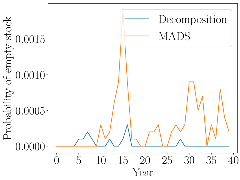
Figure 8: Evolution of the probability of having an empty stock.

Another indicator that is monitored by decision makers is the level of stock. A necessary condition for the occurrence of a forced outage is that the stock is empty. Hence, we look at the probability of having an empty stock. The higher this probability, the higher the probability of forced outage. The probability of having an empty stock is very low on the whole horizon for the decomposition strategy (Fig. 8). For MADS strategy this probability is often higher in particular around year $15$ and after year $30$. This feature again supports that the the decomposition strategy is more robust than MADS strategy.

Overall on this case, the strategy obtained by decomposition is more cost effective than MADS strategy. In the case of extreme events, the decomposition strategy is more robust than MADS strategy, as shown by the $99\%$ quantile in Table 4, the number of failures and of forced outages in Table 5 and the probability of having an empty stock in Fig. 8.

5.2.2 Results for Case 2

In the second case presented in Table 1, the components have a longer lifespan but the stock has fewer parts than in the first case. The coupling between the components and the stock is then more important than in Case 1. The mean cost of the maintenance strategy returned by MADS is $10815$ k€ and it is $9749$ k€ for the strategy returned by the decomposition, which represents a gain of $10\%$. The values of some quantiles are gathered in Table 6 and the distribution of the cost is represented on Fig. 10. The situation is quite different from the first case as the decomposition strategy has a more important variance than MADS strategy and presents several modes.

	$1\%$	$5\%$	$25\%$	$50\%$	$75\%$	$95\%$	$99\%$
Decomposition	$5381$	$5601$	$5999$	$9054$	$13014$	$18421$	$23069$
MADS	$10221$	$10357$	$10568$	$10733$	$10916$	$11266$	$13650$

Table 6: Quantiles of the cost of the two maintenance strategies (k€).

Figure 9: Distribution of the cost for the two maintenance strategies. The dashed lines represent the expected cost for both strategies.

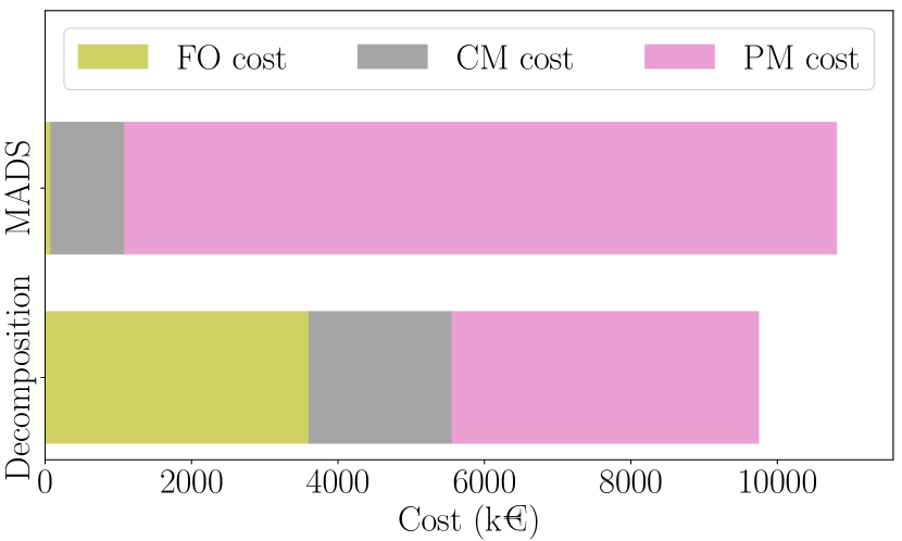
Figure 10: Part of the PM, CM and forced outage cost in the total expected cost.

The repartition of the cost in Fig. 10 confirms that the two maintenance strategies have a different approach. The strategy returned by MADS is similar than in the first case with a high number of PMs, few failures and forced outages, see Table 7. On the other hand, with the decomposition strategy the PM cost is much lower, as fewer PMs are performed (Table 7). The counterpart is a higher CM cost and a notable contribution of the forced outage cost. We see in Table 7 that the number of forced outages is indeed significantly higher with the decomposition strategy, with almost one forced outage per scenario in average. Thus, the approaches of the two maintenance strategies are completely different: the MADS strategy is conservative with a lot of PMs (similarly as in the first case) whereas the decomposition strategy is more risky with fewer PMs and more forced outages.

	Decomposition	MADS
Total number of PMs	$503$	$644$
Mean number of PMs / component	$6.3$	$8.1$
Mean number of failures / component	$0.38$	$0.26$
Number of forced outages / scenario	$0.94$	$0.04$
Computation time	$5$ days, $12$ hours	$3$ days, $12$ hours

Table 7: Number of PMs, failures and forced outages, and computation time for each strategy.

The cumulative number of PMs can be visualized on Fig. 12. Similarly as in the first case, we see a time-dependent behavior of the decomposition strategy with almost no maintenance in the first seven years. In Case 1, the decomposition strategy does not perform PMs in the first three years only but the components have a shorter average lifespan (around $9$ years in Case 1 and $18$ years in Case 2). In the first half of the time horizon, the decomposition strategy performs fewer PMs than MADS strategy, whereas in the second half of the horizon the decomposition performs slightly more PMs than MADS. We see in Fig. 12, that the decomposition strategy results in a high probability of having an empty stock between years $10$ and $15$, where most of the forced outages occur. In the first years and in the second half of the horizon, both strategies present a low risk of having an empty stock.

In Table 7, we see that the computation time are around 3 times larger than in Case 1. This is due to the fact that we have used $Q=300$ scenarios here against $Q=100$ scenarios in Case 1 for the estimation of the expected cost (see Table 1). As the decomposition designs a risky strategy, if $Q$ is kept too low, the maintenance strategy may not perform well when evaluated on the $10^{5}$ validation scenarios as extreme events are not taken into account during the optimization.

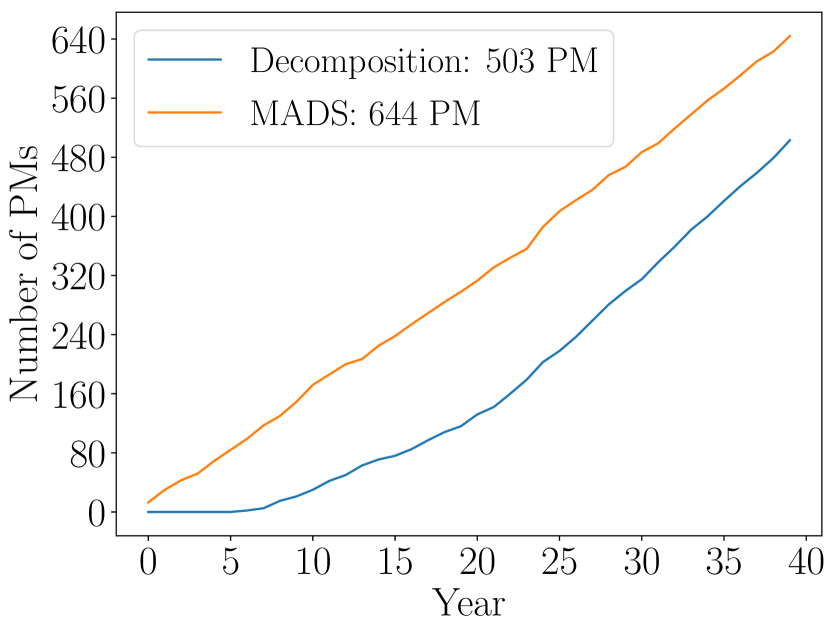
Figure 11: Cumulative number of PMs.

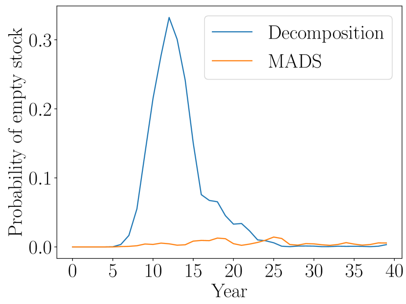
Figure 12: Evolution of the probability of having an empty stock.

Overall for this case, the decomposition strategy performs better in expectation, which is the criterion that the problem has been designed to optimize. However, the decomposition strategy has a higher variance than MADS strategy with an important risk of forced outage. Thus, from an operational point of view, a decision maker will probably choose the MADS strategy. Our work is meant to be a decision support tool and is not design to take the final operational decision. The analysis of Fig. 12 and 12 suggest to investigate a maintenance strategy that is similar to the decomposition strategy in the first years and in the second half of the horizon but with more PMs between years $10$ and $15$ to reduce the number of forced outages. We have the insight that this new strategy could improve the robustness of the decomposition strategy and perform similarly or even better in expectation.

6 Conclusion

In this work we study a maintenance scheduling optimization problem for hydropower plants management. We set up a decomposition method to find a deterministic preventive maintenance strategy for a system of physical components sharing a common stock of spare parts. The decomposition relies on the Auxiliary Problem Principle. We construct a sequence of auxiliary problems that are solved iteratively. The auxiliary problems are decomposable into independent subproblems of smaller dimension that are solved in parallel. Each subproblem involves only one component of the system or the stock. A relaxation of the system is necessary as the gradients of the dynamics and the cost are required to compute the coordination terms. Then, the fixed-point algorithm is implemented with an efficient mixed parallel/sequential strategy. This implementation is particularly adapted to the structure of the industrial problem, for which the subproblem on the stock is easy to solve numerically.

On the two industrial test cases, the decomposition method outperforms in expectation the blackbox algorithm MADS applied directly on the full problem. The reason is that when MADS is used to solve subproblems of small dimension within the decomposition algorithm, it manages to detect features to design an efficient time-dependent PM strategy. These features – such as not replacing components in the first years of the horizon – cannot be detected when MADS is applied directly on the full problem as the corresponding strategies only represent a very small subset of the search space which is not explored by the algorithm.

The approach of the decomposition strategy differs between the two test cases. In the first case the strategy is conservative and robust to extreme events whereas in the second test case, it is more risky as more forced outages can occur. Our work is meant to be a decision support tool and even if it is unlikely that a decision maker chooses a risky maintenance strategy, the results on the second case can give insights for the design of an efficient robust maintenance strategy.

This work proves the interest of the modeling effort needed to apply the decomposition method. Some challenges still remain for an application in an operational context. In order to force the design of a robust maintenance strategy, some risk criteria should be added in the mathematical formulation of the problem, either in the cost function or in the constraint. Another point that must be noticed is that the dynamics is simulated with a time step of one year. A smaller time step must be used for an accurate evaluation of the costs. This will not increase the complexity of the problem as maintenance decisions are always made on a yearly basis, so that the space of admissible maintenance strategies is still of the same dimension. However, the time needed for the evaluation of the cost function will increase. It is also possible to model more complex systems, by adding a control on the time of the order of spare parts or dependence between the failures of the components for instance. We could also consider imperfect preventive maintenance. A balance must be found between the simplicity of the model and its adequation to reality given the industrial application in mind.

Appendix A Explicit expression of the dynamics of the original system

In this part, we give an explicit expression for the dynamics $f_{i}$ of component $i\in\mathbb{I}$ that appears in (2.19). We can write:

$$\boldsymbol{X^{\textstyle\text{\unboldmath$\scriptstyle$}}_{\textstyle\text{\unboldmath$\scriptstyle i,t+1$}}}=\begin{pmatrix}\boldsymbol{E^{\textstyle\text{\unboldmath$\scriptstyle$}}_{\textstyle\text{\unboldmath$\scriptstyle i,t+1$}}}\\ \boldsymbol{A^{\textstyle\text{\unboldmath$\scriptstyle$}}_{\textstyle\text{\unboldmath$\scriptstyle i,t+1$}}}\\ \boldsymbol{P^{\textstyle\text{\unboldmath$\scriptstyle$}}_{\textstyle\text{\unboldmath$\scriptstyle i,t+1$}}}\end{pmatrix}=\begin{pmatrix}f_{i,\boldsymbol{E^{\textstyle\text{\unboldmath$\scriptstyle$}}_{\textstyle\text{\unboldmath$\scriptstyle$}}}}(\boldsymbol{X^{\textstyle\text{\unboldmath$\scriptstyle$}}_{\textstyle\text{\unboldmath$\scriptstyle 1:i,t$}}},\boldsymbol{S^{\textstyle\text{\unboldmath$\scriptstyle$}}_{\textstyle\text{\unboldmath$\scriptstyle t$}}},u_{i,t},\boldsymbol{W^{\textstyle\text{\unboldmath$\scriptstyle$}}_{\textstyle\text{\unboldmath$\scriptstyle i,t+1$}}})\\ f_{i,\boldsymbol{A^{\textstyle\text{\unboldmath$\scriptstyle$}}_{\textstyle\text{\unboldmath$\scriptstyle$}}}}(\boldsymbol{X^{\textstyle\text{\unboldmath$\scriptstyle$}}_{\textstyle\text{\unboldmath$\scriptstyle 1:i,t$}}},\boldsymbol{S^{\textstyle\text{\unboldmath$\scriptstyle$}}_{\textstyle\text{\unboldmath$\scriptstyle t$}}},u_{i,t},\boldsymbol{W^{\textstyle\text{\unboldmath$\scriptstyle$}}_{\textstyle\text{\unboldmath$\scriptstyle i,t+1$}}})\\ f_{i,\boldsymbol{P^{\textstyle\text{\unboldmath$\scriptstyle$}}_{\textstyle\text{\unboldmath$\scriptstyle$}}}}(\boldsymbol{X^{\textstyle\text{\unboldmath$\scriptstyle$}}_{\textstyle\text{\unboldmath$\scriptstyle 1:i,t$}}},\boldsymbol{S^{\textstyle\text{\unboldmath$\scriptstyle$}}_{\textstyle\text{\unboldmath$\scriptstyle t$}}},u_{i,t},\boldsymbol{W^{\textstyle\text{\unboldmath$\scriptstyle$}}_{\textstyle\text{\unboldmath$\scriptstyle i,t+1$}}})\\ \end{pmatrix}\;,$$ (A.1)

so that $f_{i}=(f_{i,\boldsymbol{E^{\textstyle\text{\unboldmath$\scriptstyle$}}_{\textstyle\text{\unboldmath$\scriptstyle$}}}},f_{i,\boldsymbol{A^{\textstyle\text{\unboldmath$\scriptstyle$}}_{\textstyle\text{\unboldmath$\scriptstyle$}}}},f_{i,\boldsymbol{P^{\textstyle\text{\unboldmath$\scriptstyle$}}_{\textstyle\text{\unboldmath$\scriptstyle$}}}})$. We give an explicit formula for $f_{i,\boldsymbol{E^{\textstyle\text{\unboldmath$\scriptstyle$}}_{\textstyle\text{\unboldmath$\scriptstyle$}}}},f_{i,\boldsymbol{A^{\textstyle\text{\unboldmath$\scriptstyle$}}_{\textstyle\text{\unboldmath$\scriptstyle$}}}}$ and $f_{i,\boldsymbol{P^{\textstyle\text{\unboldmath$\scriptstyle$}}_{\textstyle\text{\unboldmath$\scriptstyle$}}}}$.

A.1 Dynamics of the regime $\boldsymbol{E}_{i,t}$

Using Fig. 3, we can write:

$$\boldsymbol{E^{\textstyle\text{\unboldmath$\scriptstyle$}}_{\textstyle\text{\unboldmath$\scriptstyle i,t+1$}}} =f_{i,\boldsymbol{E^{\textstyle\text{\unboldmath$\scriptstyle$}}_{\textstyle\text{\unboldmath$\scriptstyle$}}}}(\boldsymbol{X^{\textstyle\text{\unboldmath$\scriptstyle$}}_{\textstyle\text{\unboldmath$\scriptstyle 1:i,t$}}},\boldsymbol{S^{\textstyle\text{\unboldmath$\scriptstyle$}}_{\textstyle\text{\unboldmath$\scriptstyle t$}}},u_{i,t},\boldsymbol{W^{\textstyle\text{\unboldmath$\scriptstyle$}}_{\textstyle\text{\unboldmath$\scriptstyle i,t+1$}}})$$ (A.2)

$$=\begin{multlined}\mathbf{1}_{\mathbb{R}_{+}}(\boldsymbol{S^{\textstyle\text{\unboldmath$\scriptstyle$}}_{\textstyle\text{\unboldmath$\scriptstyle t$}}}-\sum_{j=1}^{i}\mathbf{1}_{\{0\}}(\boldsymbol{E^{\textstyle\text{\unboldmath$\scriptstyle$}}_{\textstyle\text{\unboldmath$\scriptstyle j,t$}}}))\mathbf{1}_{\{0\}}(\boldsymbol{E^{\textstyle\text{\unboldmath$\scriptstyle$}}_{\textstyle\text{\unboldmath$\scriptstyle i,t$}}})\\ +\big{(}\mathbf{1}_{\mathbb{R}_{+}}(u_{i,t}-\nu)+\mathbf{1}_{\mathbb{R}_{+}}(\boldsymbol{W^{\textstyle\text{\unboldmath$\scriptstyle$}}_{\textstyle\text{\unboldmath$\scriptstyle i,t+1$}}}-p_{i}(\boldsymbol{A^{\textstyle\text{\unboldmath$\scriptstyle$}}_{\textstyle\text{\unboldmath$\scriptstyle i,t$}}}))\mathbf{1}_{\mathbb{R}_{+}^{*}}(\nu-u_{i,t})\big{)}\mathbf{1}_{\{1\}}(\boldsymbol{E^{\textstyle\text{\unboldmath$\scriptstyle$}}_{\textstyle\text{\unboldmath$\scriptstyle i,t$}}})\;.\end{multlined}\mathbf{1}_{\mathbb{R}_{+}}(\boldsymbol{S^{\textstyle\text{\unboldmath$\scriptstyle$}}_{\textstyle\text{\unboldmath$\scriptstyle t$}}}-\sum_{j=1}^{i}\mathbf{1}_{\{0\}}(\boldsymbol{E^{\textstyle\text{\unboldmath$\scriptstyle$}}_{\textstyle\text{\unboldmath$\scriptstyle j,t$}}}))\mathbf{1}_{\{0\}}(\boldsymbol{E^{\textstyle\text{\unboldmath$\scriptstyle$}}_{\textstyle\text{\unboldmath$\scriptstyle i,t$}}})\\ +\big{(}\mathbf{1}_{\mathbb{R}_{+}}(u_{i,t}-\nu)+\mathbf{1}_{\mathbb{R}_{+}}(\boldsymbol{W^{\textstyle\text{\unboldmath$\scriptstyle$}}_{\textstyle\text{\unboldmath$\scriptstyle i,t+1$}}}-p_{i}(\boldsymbol{A^{\textstyle\text{\unboldmath$\scriptstyle$}}_{\textstyle\text{\unboldmath$\scriptstyle i,t$}}}))\mathbf{1}_{\mathbb{R}_{+}^{*}}(\nu-u_{i,t})\big{)}\mathbf{1}_{\{1\}}(\boldsymbol{E^{\textstyle\text{\unboldmath$\scriptstyle$}}_{\textstyle\text{\unboldmath$\scriptstyle i,t$}}})\;.$$

The first part of (A.2) means that if the component is broken at $t$ and we have enough spares to repair it, it is then functioning at $t+1$. The second part means that if the component is functioning at $t$ and we do a PM, it is still functioning at $t+1$. Finally, if we do not do a PM, the regime depends on the occurrence of a failure between $t$ and $t+1$.

A.2 Dynamics of the age $\boldsymbol{A}_{i,t}$

Again using Fig. 3, we can write:

$$\boldsymbol{A^{\textstyle\text{\unboldmath$\scriptstyle$}}_{\textstyle\text{\unboldmath$\scriptstyle i,t+1$}}} =f_{i,\boldsymbol{A^{\textstyle\text{\unboldmath$\scriptstyle$}}_{\textstyle\text{\unboldmath$\scriptstyle$}}}}(\boldsymbol{X^{\textstyle\text{\unboldmath$\scriptstyle$}}_{\textstyle\text{\unboldmath$\scriptstyle 1:i,t$}}},\boldsymbol{S^{\textstyle\text{\unboldmath$\scriptstyle$}}_{\textstyle\text{\unboldmath$\scriptstyle t$}}},u_{i,t},\boldsymbol{W^{\textstyle\text{\unboldmath$\scriptstyle$}}_{\textstyle\text{\unboldmath$\scriptstyle i,t+1$}}})$$ (A.3)

$$=\begin{multlined}(\boldsymbol{A^{\textstyle\text{\unboldmath$\scriptstyle$}}_{\textstyle\text{\unboldmath$\scriptstyle i,t$}}}+1)\bigg{(}\mathbf{1}_{\mathbb{R}_{+}^{*}}(\sum_{j=1}^{i}\mathbf{1}_{\{0\}}(\boldsymbol{E^{\textstyle\text{\unboldmath$\scriptstyle$}}_{\textstyle\text{\unboldmath$\scriptstyle j,t$}}})-\boldsymbol{S^{\textstyle\text{\unboldmath$\scriptstyle$}}_{\textstyle\text{\unboldmath$\scriptstyle t$}}})\mathbf{1}_{\{0\}}(\boldsymbol{E^{\textstyle\text{\unboldmath$\scriptstyle$}}_{\textstyle\text{\unboldmath$\scriptstyle i,t$}}})\\ +\mathbf{1}_{\mathbb{R}_{+}}(\boldsymbol{W^{\textstyle\text{\unboldmath$\scriptstyle$}}_{\textstyle\text{\unboldmath$\scriptstyle i,t+1$}}}-p_{i}(\boldsymbol{A^{\textstyle\text{\unboldmath$\scriptstyle$}}_{\textstyle\text{\unboldmath$\scriptstyle i,t$}}}))\mathbf{1}_{\mathbb{R}_{+}^{*}}(\nu-u_{i,t})\mathbf{1}_{\{1\}}(\boldsymbol{E^{\textstyle\text{\unboldmath$\scriptstyle$}}_{\textstyle\text{\unboldmath$\scriptstyle i,t$}}})\bigg{)}\\ +\mathbf{1}_{\mathbb{R}_{+}}(\boldsymbol{S^{\textstyle\text{\unboldmath$\scriptstyle$}}_{\textstyle\text{\unboldmath$\scriptstyle t$}}}-\sum_{j=1}^{i}\mathbf{1}_{\{0\}}(\boldsymbol{E^{\textstyle\text{\unboldmath$\scriptstyle$}}_{\textstyle\text{\unboldmath$\scriptstyle j,t$}}}))\mathbf{1}_{\{0\}}(\boldsymbol{E^{\textstyle\text{\unboldmath$\scriptstyle$}}_{\textstyle\text{\unboldmath$\scriptstyle i,t$}}})+\left((1-u_{i,t})\boldsymbol{A^{\textstyle\text{\unboldmath$\scriptstyle$}}_{\textstyle\text{\unboldmath$\scriptstyle i,t$}}}+1\right)\mathbf{1}_{\mathbb{R}_{+}}(u_{i,t}-\nu)\mathbf{1}_{\{1\}}(\boldsymbol{E^{\textstyle\text{\unboldmath$\scriptstyle$}}_{\textstyle\text{\unboldmath$\scriptstyle i,t$}}})\;.\end{multlined}(\boldsymbol{A^{\textstyle\text{\unboldmath$\scriptstyle$}}_{\textstyle\text{\unboldmath$\scriptstyle i,t$}}}+1)\bigg{(}\mathbf{1}_{\mathbb{R}_{+}^{*}}(\sum_{j=1}^{i}\mathbf{1}_{\{0\}}(\boldsymbol{E^{\textstyle\text{\unboldmath$\scriptstyle$}}_{\textstyle\text{\unboldmath$\scriptstyle j,t$}}})-\boldsymbol{S^{\textstyle\text{\unboldmath$\scriptstyle$}}_{\textstyle\text{\unboldmath$\scriptstyle t$}}})\mathbf{1}_{\{0\}}(\boldsymbol{E^{\textstyle\text{\unboldmath$\scriptstyle$}}_{\textstyle\text{\unboldmath$\scriptstyle i,t$}}})\\ +\mathbf{1}_{\mathbb{R}_{+}}(\boldsymbol{W^{\textstyle\text{\unboldmath$\scriptstyle$}}_{\textstyle\text{\unboldmath$\scriptstyle i,t+1$}}}-p_{i}(\boldsymbol{A^{\textstyle\text{\unboldmath$\scriptstyle$}}_{\textstyle\text{\unboldmath$\scriptstyle i,t$}}}))\mathbf{1}_{\mathbb{R}_{+}^{*}}(\nu-u_{i,t})\mathbf{1}_{\{1\}}(\boldsymbol{E^{\textstyle\text{\unboldmath$\scriptstyle$}}_{\textstyle\text{\unboldmath$\scriptstyle i,t$}}})\bigg{)}\\ +\mathbf{1}_{\mathbb{R}_{+}}(\boldsymbol{S^{\textstyle\text{\unboldmath$\scriptstyle$}}_{\textstyle\text{\unboldmath$\scriptstyle t$}}}-\sum_{j=1}^{i}\mathbf{1}_{\{0\}}(\boldsymbol{E^{\textstyle\text{\unboldmath$\scriptstyle$}}_{\textstyle\text{\unboldmath$\scriptstyle j,t$}}}))\mathbf{1}_{\{0\}}(\boldsymbol{E^{\textstyle\text{\unboldmath$\scriptstyle$}}_{\textstyle\text{\unboldmath$\scriptstyle i,t$}}})+\left((1-u_{i,t})\boldsymbol{A^{\textstyle\text{\unboldmath$\scriptstyle$}}_{\textstyle\text{\unboldmath$\scriptstyle i,t$}}}+1\right)\mathbf{1}_{\mathbb{R}_{+}}(u_{i,t}-\nu)\mathbf{1}_{\{1\}}(\boldsymbol{E^{\textstyle\text{\unboldmath$\scriptstyle$}}_{\textstyle\text{\unboldmath$\scriptstyle i,t$}}})\;.$$

If the component is broken at $t$, it stays broken if there are not enough spares in the stock (first line of (A.3)). In this case the time $\boldsymbol{A^{\textstyle\text{\unboldmath$\scriptstyle$}}_{\textstyle\text{\unboldmath$\scriptstyle i,t$}}}$ increases by $1$. If the component is healthy at $t$, it ages if no PM is done and no failure occurs (second line of (A.3)). When the component is broken and that there are enough spares (first term in the third line of (A.3)), a CM is performed and we have $\boldsymbol{A^{\textstyle\text{\unboldmath$\scriptstyle$}}_{\textstyle\text{\unboldmath$\scriptstyle i,t+1$}}}=1$. In the case of a PM (second term in the third line of (A.3)), the component is rejuvenated and its age becomes $\boldsymbol{A^{\textstyle\text{\unboldmath$\scriptstyle$}}_{\textstyle\text{\unboldmath$\scriptstyle i,t+1$}}}=(1-u_{i,t})\boldsymbol{A^{\textstyle\text{\unboldmath$\scriptstyle$}}_{\textstyle\text{\unboldmath$\scriptstyle i,t$}}}+1$. If there is a failure, we have $\boldsymbol{A^{\textstyle\text{\unboldmath$\scriptstyle$}}_{\textstyle\text{\unboldmath$\scriptstyle i,t+1$}}}=0$.

A.3 Dynamics of the vector of times since last failures $\boldsymbol{P}_{i,t}$

The expression of the dynamics of $\boldsymbol{P^{\textstyle\text{\unboldmath$\scriptstyle$}}_{\textstyle\text{\unboldmath$\scriptstyle i,t$}}}=(\boldsymbol{P^{\textstyle\text{\unboldmath$\scriptstyle 1$}}_{\textstyle\text{\unboldmath$\scriptstyle i,t$}}},\ldots,\boldsymbol{P^{\textstyle\text{\unboldmath$\scriptstyle D$}}_{\textstyle\text{\unboldmath$\scriptstyle i,t$}}})$ is more complex. We write:

$$\boldsymbol{P^{\textstyle\text{\unboldmath$\scriptstyle$}}_{\textstyle\text{\unboldmath$\scriptstyle i,t+1$}}} =\begin{pmatrix}\boldsymbol{P^{\textstyle\text{\unboldmath$\scriptstyle 1$}}_{\textstyle\text{\unboldmath$\scriptstyle i,t+1$}}}\\ \vdots\\ \boldsymbol{P^{\textstyle\text{\unboldmath$\scriptstyle D$}}_{\textstyle\text{\unboldmath$\scriptstyle i,t+1$}}}\end{pmatrix}=\begin{pmatrix}f_{i,\boldsymbol{P^{\textstyle\text{\unboldmath$\scriptstyle$}}_{\textstyle\text{\unboldmath$\scriptstyle$}}}}^{1}(\boldsymbol{X^{\textstyle\text{\unboldmath$\scriptstyle$}}_{\textstyle\text{\unboldmath$\scriptstyle 1:i,t$}}},\boldsymbol{S^{\textstyle\text{\unboldmath$\scriptstyle$}}_{\textstyle\text{\unboldmath$\scriptstyle t$}}},u_{i,t},\boldsymbol{W^{\textstyle\text{\unboldmath$\scriptstyle$}}_{\textstyle\text{\unboldmath$\scriptstyle i,t+1$}}})\\ \vdots\\ f_{i,\boldsymbol{P^{\textstyle\text{\unboldmath$\scriptstyle$}}_{\textstyle\text{\unboldmath$\scriptstyle$}}}}^{D}(\boldsymbol{X^{\textstyle\text{\unboldmath$\scriptstyle$}}_{\textstyle\text{\unboldmath$\scriptstyle 1:i,t$}}},\boldsymbol{S^{\textstyle\text{\unboldmath$\scriptstyle$}}_{\textstyle\text{\unboldmath$\scriptstyle t$}}},u_{i,t},\boldsymbol{W^{\textstyle\text{\unboldmath$\scriptstyle$}}_{\textstyle\text{\unboldmath$\scriptstyle i,t+1$}}})\end{pmatrix}=f_{i,\boldsymbol{P^{\textstyle\text{\unboldmath$\scriptstyle$}}_{\textstyle\text{\unboldmath$\scriptstyle$}}}}(\boldsymbol{X^{\textstyle\text{\unboldmath$\scriptstyle$}}_{\textstyle\text{\unboldmath$\scriptstyle 1:i,t$}}},\boldsymbol{S^{\textstyle\text{\unboldmath$\scriptstyle$}}_{\textstyle\text{\unboldmath$\scriptstyle t$}}},u_{i,t},\boldsymbol{W^{\textstyle\text{\unboldmath$\scriptstyle$}}_{\textstyle\text{\unboldmath$\scriptstyle i,t+1$}}})\;,$$ (A.4)

so that $$f_{i,\boldsymbol{P^{\textstyle\text{\unboldmath$\scriptstyle$}}_{\textstyle\text{\unboldmath$\scriptstyle$}}}}=(f_{i,\boldsymbol{P^{\textstyle\text{\unboldmath$\scriptstyle$}}_{\textstyle\text{\unboldmath$\scriptstyle$}}}}^{1},\ldots,f_{i,\boldsymbol{P^{\textstyle\text{\unboldmath$\scriptstyle$}}_{\textstyle\text{\unboldmath$\scriptstyle$}}}}^{D}) f_{i,\boldsymbol{P^{\textstyle\text{\unboldmath$\scriptstyle$}}_{\textstyle\text{\unboldmath$\scriptstyle$}}}}^{d} d\in\{1,\ldots,D\}$$. We give the expression of for :

$$\boldsymbol{P^{\textstyle\text{\unboldmath$\scriptstyle d$}}_{\textstyle\text{\unboldmath$\scriptstyle i,t+1$}}} =\begin{multlined}\Big{(}(\boldsymbol{P^{\textstyle\text{\unboldmath$\scriptstyle d$}}_{\textstyle\text{\unboldmath$\scriptstyle i,t$}}}+1)\mathbf{1}_{\mathbb{R}_{+}}(\boldsymbol{P^{\textstyle\text{\unboldmath$\scriptstyle d$}}_{\textstyle\text{\unboldmath$\scriptstyle i,t$}}})+\delta\mathbf{1}_{\{\delta\}}(\boldsymbol{P^{\textstyle\text{\unboldmath$\scriptstyle d$}}_{\textstyle\text{\unboldmath$\scriptstyle i,t$}}})\Big{)}\Big{(}1-\mathbf{1}_{\{1\}}(\boldsymbol{E^{\textstyle\text{\unboldmath$\scriptstyle$}}_{\textstyle\text{\unboldmath$\scriptstyle i,t$}}})\mathbf{1}_{\{0\}}(\boldsymbol{E^{\textstyle\text{\unboldmath$\scriptstyle$}}_{\textstyle\text{\unboldmath$\scriptstyle i,t+1$}}})\Big{)}\\ +\Big{(}(\boldsymbol{P^{\textstyle\text{\unboldmath$\scriptstyle d$}}_{\textstyle\text{\unboldmath$\scriptstyle i,t$}}}+1)\mathbf{1}_{\mathbb{R}_{+}}(\boldsymbol{P^{\textstyle\text{\unboldmath$\scriptstyle d$}}_{\textstyle\text{\unboldmath$\scriptstyle i,t$}}})\mathbf{1}_{\{\delta\}}(\boldsymbol{P^{\textstyle\text{\unboldmath$\scriptstyle D$}}_{\textstyle\text{\unboldmath$\scriptstyle i,t$}}})+\delta\mathbf{1}_{\{\delta\}}(\boldsymbol{P^{\textstyle\text{\unboldmath$\scriptstyle d-1$}}_{\textstyle\text{\unboldmath$\scriptstyle i,t$}}})\mathbf{1}_{[2,D]}(d)\\ +(\boldsymbol{P^{\textstyle\text{\unboldmath$\scriptstyle d+1$}}_{\textstyle\text{\unboldmath$\scriptstyle i,t$}}}+1)\mathbf{1}_{\mathbb{R}_{+}}(\boldsymbol{P^{\textstyle\text{\unboldmath$\scriptstyle D$}}_{\textstyle\text{\unboldmath$\scriptstyle i,t$}}})\mathbf{1}_{[1,D-1]}(d)\Big{)}\mathbf{1}_{\{1\}}(\boldsymbol{E^{\textstyle\text{\unboldmath$\scriptstyle$}}_{\textstyle\text{\unboldmath$\scriptstyle i,t$}}})\mathbf{1}_{\{0\}}(\boldsymbol{E^{\textstyle\text{\unboldmath$\scriptstyle$}}_{\textstyle\text{\unboldmath$\scriptstyle i,t+1$}}})\;.\end{multlined}\Big{(}(\boldsymbol{P^{\textstyle\text{\unboldmath$\scriptstyle d$}}_{\textstyle\text{\unboldmath$\scriptstyle i,t$}}}+1)\mathbf{1}_{\mathbb{R}_{+}}(\boldsymbol{P^{\textstyle\text{\unboldmath$\scriptstyle d$}}_{\textstyle\text{\unboldmath$\scriptstyle i,t$}}})+\delta\mathbf{1}_{\{\delta\}}(\boldsymbol{P^{\textstyle\text{\unboldmath$\scriptstyle d$}}_{\textstyle\text{\unboldmath$\scriptstyle i,t$}}})\Big{)}\Big{(}1-\mathbf{1}_{\{1\}}(\boldsymbol{E^{\textstyle\text{\unboldmath$\scriptstyle$}}_{\textstyle\text{\unboldmath$\scriptstyle i,t$}}})\mathbf{1}_{\{0\}}(\boldsymbol{E^{\textstyle\text{\unboldmath$\scriptstyle$}}_{\textstyle\text{\unboldmath$\scriptstyle i,t+1$}}})\Big{)}\\ +\Big{(}(\boldsymbol{P^{\textstyle\text{\unboldmath$\scriptstyle d$}}_{\textstyle\text{\unboldmath$\scriptstyle i,t$}}}+1)\mathbf{1}_{\mathbb{R}_{+}}(\boldsymbol{P^{\textstyle\text{\unboldmath$\scriptstyle d$}}_{\textstyle\text{\unboldmath$\scriptstyle i,t$}}})\mathbf{1}_{\{\delta\}}(\boldsymbol{P^{\textstyle\text{\unboldmath$\scriptstyle D$}}_{\textstyle\text{\unboldmath$\scriptstyle i,t$}}})+\delta\mathbf{1}_{\{\delta\}}(\boldsymbol{P^{\textstyle\text{\unboldmath$\scriptstyle d-1$}}_{\textstyle\text{\unboldmath$\scriptstyle i,t$}}})\mathbf{1}_{[2,D]}(d)\\ +(\boldsymbol{P^{\textstyle\text{\unboldmath$\scriptstyle d+1$}}_{\textstyle\text{\unboldmath$\scriptstyle i,t$}}}+1)\mathbf{1}_{\mathbb{R}_{+}}(\boldsymbol{P^{\textstyle\text{\unboldmath$\scriptstyle D$}}_{\textstyle\text{\unboldmath$\scriptstyle i,t$}}})\mathbf{1}_{[1,D-1]}(d)\Big{)}\mathbf{1}_{\{1\}}(\boldsymbol{E^{\textstyle\text{\unboldmath$\scriptstyle$}}_{\textstyle\text{\unboldmath$\scriptstyle i,t$}}})\mathbf{1}_{\{0\}}(\boldsymbol{E^{\textstyle\text{\unboldmath$\scriptstyle$}}_{\textstyle\text{\unboldmath$\scriptstyle i,t+1$}}})\;.$$ (A.8)

The first line represents the case where there is no failure. Then $\boldsymbol{P^{\textstyle\text{\unboldmath$\scriptstyle$}}_{\textstyle\text{\unboldmath$\scriptstyle i,t$}}}$ increases by one if it is different from $\delta$, otherwise it keeps the value $\delta$. When there is a failure, if component $i$ has undergone fewer than $D$ failures, the evolution of $\boldsymbol{P^{\textstyle\text{\unboldmath$\scriptstyle$}}_{\textstyle\text{\unboldmath$\scriptstyle i,t$}}}$ is described by (2.16a). This case is represented by the second line of (A.8). When the component has already undergone $D$ failures, the evolution of $\boldsymbol{P^{\textstyle\text{\unboldmath$\scriptstyle$}}_{\textstyle\text{\unboldmath$\scriptstyle i,t$}}}$ is described by (2.17a). This case is represented by the third line of (A.8). Note that this expression of $\boldsymbol{P^{\textstyle\text{\unboldmath$\scriptstyle d$}}_{\textstyle\text{\unboldmath$\scriptstyle i,t+1$}}}$ depends on $\boldsymbol{E^{\textstyle\text{\unboldmath$\scriptstyle$}}_{\textstyle\text{\unboldmath$\scriptstyle i,t+1$}}}$. It is possible to express $\boldsymbol{P^{\textstyle\text{\unboldmath$\scriptstyle d$}}_{\textstyle\text{\unboldmath$\scriptstyle i,t+1$}}}$ only with variables describing component $i$ at time $t$, this can be done by replacing $\boldsymbol{E^{\textstyle\text{\unboldmath$\scriptstyle$}}_{\textstyle\text{\unboldmath$\scriptstyle i,t+1$}}}$ by its expression (A.2).

A.4 Dynamics of the stock $\boldsymbol{S}_{t}$

We recall the explicit dynamics of the stock that is already given in (2.20):

$$\boldsymbol{S^{\textstyle\text{\unboldmath$\scriptstyle$}}_{\textstyle\text{\unboldmath$\scriptstyle t+1$}}}=\boldsymbol{S^{\textstyle\text{\unboldmath$\scriptstyle$}}_{\textstyle\text{\unboldmath$\scriptstyle t$}}}+\sum_{i=1}^{n}\sum_{d=1}^{D}\mathbf{1}_{\{D-1\}}(\boldsymbol{P^{\textstyle\text{\unboldmath$\scriptstyle d$}}_{\textstyle\text{\unboldmath$\scriptstyle i,t$}}})-\min\left\{\boldsymbol{S^{\textstyle\text{\unboldmath$\scriptstyle$}}_{\textstyle\text{\unboldmath$\scriptstyle t$}}},\ \sum_{i=1}^{n}\mathbf{1}_{\{0\}}(\boldsymbol{E^{\textstyle\text{\unboldmath$\scriptstyle$}}_{\textstyle\text{\unboldmath$\scriptstyle i,t$}}})\right\}\;.$$ (A.9)

The dynamics of the whole system has now been explicitly described.

Appendix B Explicit expression of the dynamics of the relaxed system

The expression of the relaxed dynamics of parameter $\alpha$ is obtained from Equations (A.2), (A.3), (A.8) and (A.9) by replacing the indicator function with its relaxed version.

We do not always substitute directly the indicator with its relaxation. The dynamics often involves conditions on complementary events. For example, the condition if the component is broken is represented by $\mathbf{1}_{\{0\}}(\boldsymbol{E^{\textstyle\text{\unboldmath$\scriptstyle$}}_{\textstyle\text{\unboldmath$\scriptstyle i,t$}}})$. On the other hand, the condition if the component is healthy is represented by $\mathbf{1}_{\{1\}}(\boldsymbol{E^{\textstyle\text{\unboldmath$\scriptstyle$}}_{\textstyle\text{\unboldmath$\scriptstyle i,t$}}})$. For the original dynamics as $\boldsymbol{E^{\textstyle\text{\unboldmath$\scriptstyle$}}_{\textstyle\text{\unboldmath$\scriptstyle i,t$}}}\in\{0,1\}$ we always have

$$\mathbf{1}_{\{0\}}(\boldsymbol{E^{\textstyle\text{\unboldmath$\scriptstyle$}}_{\textstyle\text{\unboldmath$\scriptstyle i,t$}}})+\mathbf{1}_{\{1\}}(\boldsymbol{E^{\textstyle\text{\unboldmath$\scriptstyle$}}_{\textstyle\text{\unboldmath$\scriptstyle i,t$}}})=1\;.$$ (B.1)

This relation is not true anymore using directly the relaxed version of the indicator with the relaxed variables. Take for example $\alpha=2$, and suppose $\boldsymbol{E^{\textstyle\text{\unboldmath$\scriptstyle$}}_{\textstyle\text{\unboldmath$\scriptstyle i,t$}}}=\frac{1}{2}$, then

$$\mathbf{1}_{\{0\}}^{\alpha}(\boldsymbol{E^{\textstyle\text{\unboldmath$\scriptstyle$}}_{\textstyle\text{\unboldmath$\scriptstyle i,t$}}})+\mathbf{1}_{\{1\}}^{\alpha}(\boldsymbol{E^{\textstyle\text{\unboldmath$\scriptstyle$}}_{\textstyle\text{\unboldmath$\scriptstyle i,t$}}})=0\;.$$ (B.2)

If we replace directly all indicator functions by their relaxation, the consequence would be in this case that $\boldsymbol{E^{\textstyle\text{\unboldmath$\scriptstyle$}}_{\textstyle\text{\unboldmath$\scriptstyle i,t+1$}}}=0$ no matter the control $u_{i,t}$. This means that even if we do a PM with $u_{i,t}=1$, the component is down at $t+1$. This does not represent the dynamics of the system as we would expect. To design a coherent relaxed dynamics, complementary conditions $\mathbf{1}_{\mathcal{A}}$ and $\mathbf{1}_{\mathcal{A}^{\mathrm{c}}}$ are represented using the relaxed version $\mathbf{1}_{\mathcal{A}}^{\alpha}$ of the indicator function for the first condition and the function $1-\mathbf{1}_{\mathcal{A}}^{\alpha}$ for the complementary condition.

B.1 Relaxed dynamics of the regime $\boldsymbol{E}_{i,t}$

The relaxed dynamics of the regime of parameter $\alpha>0$ is given by:

$$\boldsymbol{E^{\textstyle\text{\unboldmath$\scriptstyle$}}_{\textstyle\text{\unboldmath$\scriptstyle i,t+1$}}} =f_{i,\boldsymbol{E^{\textstyle\text{\unboldmath$\scriptstyle$}}_{\textstyle\text{\unboldmath$\scriptstyle$}}}}^{\alpha}(\boldsymbol{X^{\textstyle\text{\unboldmath$\scriptstyle$}}_{\textstyle\text{\unboldmath$\scriptstyle 1:i,t$}}},\boldsymbol{S^{\textstyle\text{\unboldmath$\scriptstyle$}}_{\textstyle\text{\unboldmath$\scriptstyle t$}}},u_{i,t},\boldsymbol{W^{\textstyle\text{\unboldmath$\scriptstyle$}}_{\textstyle\text{\unboldmath$\scriptstyle i,t+1$}}})$$ (B.3)

$$=\begin{multlined}\mathbf{1}_{\mathbb{R}_{+}}^{\alpha}(\boldsymbol{S^{\textstyle\text{\unboldmath$\scriptstyle$}}_{\textstyle\text{\unboldmath$\scriptstyle t$}}}-\sum_{j=1}^{i}\mathbf{1}_{\{0\}}^{\alpha}(\boldsymbol{E^{\textstyle\text{\unboldmath$\scriptstyle$}}_{\textstyle\text{\unboldmath$\scriptstyle j,t$}}}))\mathbf{1}_{\{0\}}^{\alpha}(\boldsymbol{E^{\textstyle\text{\unboldmath$\scriptstyle$}}_{\textstyle\text{\unboldmath$\scriptstyle i,t$}}})+\Big{(}\mathbf{1}_{\mathbb{R}_{+}}^{\alpha}(u_{i,t}-\nu)\\ +\mathbf{1}_{\mathbb{R}_{+}}^{\alpha}(\boldsymbol{W^{\textstyle\text{\unboldmath$\scriptstyle$}}_{\textstyle\text{\unboldmath$\scriptstyle i,t+1$}}}-p_{i}(\boldsymbol{A^{\textstyle\text{\unboldmath$\scriptstyle$}}_{\textstyle\text{\unboldmath$\scriptstyle i,t$}}}))(1-\mathbf{1}_{\mathbb{R}_{+}}^{\alpha}(u_{i,t}-\nu))\Big{)}\left(1-\mathbf{1}_{\{0\}}^{\alpha}(\boldsymbol{E^{\textstyle\text{\unboldmath$\scriptstyle$}}_{\textstyle\text{\unboldmath$\scriptstyle i,t$}}})\right)\;.\end{multlined}\mathbf{1}_{\mathbb{R}_{+}}^{\alpha}(\boldsymbol{S^{\textstyle\text{\unboldmath$\scriptstyle$}}_{\textstyle\text{\unboldmath$\scriptstyle t$}}}-\sum_{j=1}^{i}\mathbf{1}_{\{0\}}^{\alpha}(\boldsymbol{E^{\textstyle\text{\unboldmath$\scriptstyle$}}_{\textstyle\text{\unboldmath$\scriptstyle j,t$}}}))\mathbf{1}_{\{0\}}^{\alpha}(\boldsymbol{E^{\textstyle\text{\unboldmath$\scriptstyle$}}_{\textstyle\text{\unboldmath$\scriptstyle i,t$}}})+\Big{(}\mathbf{1}_{\mathbb{R}_{+}}^{\alpha}(u_{i,t}-\nu)\\ +\mathbf{1}_{\mathbb{R}_{+}}^{\alpha}(\boldsymbol{W^{\textstyle\text{\unboldmath$\scriptstyle$}}_{\textstyle\text{\unboldmath$\scriptstyle i,t+1$}}}-p_{i}(\boldsymbol{A^{\textstyle\text{\unboldmath$\scriptstyle$}}_{\textstyle\text{\unboldmath$\scriptstyle i,t$}}}))(1-\mathbf{1}_{\mathbb{R}_{+}}^{\alpha}(u_{i,t}-\nu))\Big{)}\left(1-\mathbf{1}_{\{0\}}^{\alpha}(\boldsymbol{E^{\textstyle\text{\unboldmath$\scriptstyle$}}_{\textstyle\text{\unboldmath$\scriptstyle i,t$}}})\right)\;.$$

We use the relaxed version of the indicator for $\mathbf{1}_{\{0\}}(\boldsymbol{E^{\textstyle\text{\unboldmath$\scriptstyle$}}_{\textstyle\text{\unboldmath$\scriptstyle i,t$}}})$ and $\mathbf{1}_{\mathbb{R}_{+}}(u_{i,t}-\nu)$. We relax $\mathbf{1}_{\{1\}}(\boldsymbol{E^{\textstyle\text{\unboldmath$\scriptstyle$}}_{\textstyle\text{\unboldmath$\scriptstyle i,t$}}})$ and $\mathbf{1}_{\mathbb{R}_{+}^{*}}(\nu-u_{i,t})$ as $1-\mathbf{1}_{\{0\}}^{\alpha}(\boldsymbol{E^{\textstyle\text{\unboldmath$\scriptstyle$}}_{\textstyle\text{\unboldmath$\scriptstyle i,t$}}})$ and $1-\mathbf{1}_{\mathbb{R}_{+}}^{\alpha}(u_{i,t}-\nu)$ respectively.

B.2 Relaxed dynamics of the age $\boldsymbol{A}_{i,t}$

The relaxed dynamics of the age of parameter $\alpha>0$ is given by:

$$\boldsymbol{A^{\textstyle\text{\unboldmath$\scriptstyle$}}_{\textstyle\text{\unboldmath$\scriptstyle i,t+1$}}} =f_{i,\boldsymbol{A^{\textstyle\text{\unboldmath$\scriptstyle$}}_{\textstyle\text{\unboldmath$\scriptstyle$}}}}^{\alpha}(\boldsymbol{X^{\textstyle\text{\unboldmath$\scriptstyle$}}_{\textstyle\text{\unboldmath$\scriptstyle 1:i,t$}}},\boldsymbol{S^{\textstyle\text{\unboldmath$\scriptstyle$}}_{\textstyle\text{\unboldmath$\scriptstyle t$}}},u_{i,t},\boldsymbol{W^{\textstyle\text{\unboldmath$\scriptstyle$}}_{\textstyle\text{\unboldmath$\scriptstyle i,t+1$}}})$$ (B.4)

$$=\begin{multlined}(\boldsymbol{A^{\textstyle\text{\unboldmath$\scriptstyle$}}_{\textstyle\text{\unboldmath$\scriptstyle i,t$}}}+1)\bigg{[}\mathbf{1}_{\mathbb{R}_{+}^{*}}^{\alpha}(\sum_{j=1}^{i}\mathbf{1}_{\{0\}}^{\alpha}(\boldsymbol{E^{\textstyle\text{\unboldmath$\scriptstyle$}}_{\textstyle\text{\unboldmath$\scriptstyle j,t$}}})-\boldsymbol{S^{\textstyle\text{\unboldmath$\scriptstyle$}}_{\textstyle\text{\unboldmath$\scriptstyle t$}}})\mathbf{1}_{\{0\}}^{\alpha}(\boldsymbol{E^{\textstyle\text{\unboldmath$\scriptstyle$}}_{\textstyle\text{\unboldmath$\scriptstyle i,t$}}})\\ +\mathbf{1}_{\mathbb{R}_{+}}^{\alpha}(\boldsymbol{W^{\textstyle\text{\unboldmath$\scriptstyle$}}_{\textstyle\text{\unboldmath$\scriptstyle i,t+1$}}}-p_{i}(\boldsymbol{A^{\textstyle\text{\unboldmath$\scriptstyle$}}_{\textstyle\text{\unboldmath$\scriptstyle i,t$}}}))(1-\mathbf{1}_{\mathbb{R}_{+}}^{\alpha}(u_{i,t}-\nu))\big{(}1-\mathbf{1}_{\{0\}}^{\alpha}(\boldsymbol{E^{\textstyle\text{\unboldmath$\scriptstyle$}}_{\textstyle\text{\unboldmath$\scriptstyle i,t$}}})\big{)}\bigg{]}\\ +\big{(}1-\mathbf{1}_{\mathbb{R}_{+}^{*}}^{\alpha}(\sum_{j=1}^{i}\mathbf{1}_{\{0\}}^{\alpha}(\boldsymbol{E^{\textstyle\text{\unboldmath$\scriptstyle$}}_{\textstyle\text{\unboldmath$\scriptstyle j,t$}}})-\boldsymbol{S^{\textstyle\text{\unboldmath$\scriptstyle$}}_{\textstyle\text{\unboldmath$\scriptstyle t$}}})\big{)}\mathbf{1}_{\{0\}}^{\alpha}(\boldsymbol{E^{\textstyle\text{\unboldmath$\scriptstyle$}}_{\textstyle\text{\unboldmath$\scriptstyle i,t$}}})\\ +\left((1-u_{i,t})\boldsymbol{A^{\textstyle\text{\unboldmath$\scriptstyle$}}_{\textstyle\text{\unboldmath$\scriptstyle i,t$}}}+1\right)\mathbf{1}_{\mathbb{R}_{+}}^{\alpha}(u_{i,t}-\nu)\big{(}1-\mathbf{1}_{\{0\}}^{\alpha}(\boldsymbol{E^{\textstyle\text{\unboldmath$\scriptstyle$}}_{\textstyle\text{\unboldmath$\scriptstyle i,t$}}})\big{)}\;.\end{multlined}(\boldsymbol{A^{\textstyle\text{\unboldmath$\scriptstyle$}}_{\textstyle\text{\unboldmath$\scriptstyle i,t$}}}+1)\bigg{[}\mathbf{1}_{\mathbb{R}_{+}^{*}}^{\alpha}(\sum_{j=1}^{i}\mathbf{1}_{\{0\}}^{\alpha}(\boldsymbol{E^{\textstyle\text{\unboldmath$\scriptstyle$}}_{\textstyle\text{\unboldmath$\scriptstyle j,t$}}})-\boldsymbol{S^{\textstyle\text{\unboldmath$\scriptstyle$}}_{\textstyle\text{\unboldmath$\scriptstyle t$}}})\mathbf{1}_{\{0\}}^{\alpha}(\boldsymbol{E^{\textstyle\text{\unboldmath$\scriptstyle$}}_{\textstyle\text{\unboldmath$\scriptstyle i,t$}}})\\ +\mathbf{1}_{\mathbb{R}_{+}}^{\alpha}(\boldsymbol{W^{\textstyle\text{\unboldmath$\scriptstyle$}}_{\textstyle\text{\unboldmath$\scriptstyle i,t+1$}}}-p_{i}(\boldsymbol{A^{\textstyle\text{\unboldmath$\scriptstyle$}}_{\textstyle\text{\unboldmath$\scriptstyle i,t$}}}))(1-\mathbf{1}_{\mathbb{R}_{+}}^{\alpha}(u_{i,t}-\nu))\big{(}1-\mathbf{1}_{\{0\}}^{\alpha}(\boldsymbol{E^{\textstyle\text{\unboldmath$\scriptstyle$}}_{\textstyle\text{\unboldmath$\scriptstyle i,t$}}})\big{)}\bigg{]}\\ +\big{(}1-\mathbf{1}_{\mathbb{R}_{+}^{*}}^{\alpha}(\sum_{j=1}^{i}\mathbf{1}_{\{0\}}^{\alpha}(\boldsymbol{E^{\textstyle\text{\unboldmath$\scriptstyle$}}_{\textstyle\text{\unboldmath$\scriptstyle j,t$}}})-\boldsymbol{S^{\textstyle\text{\unboldmath$\scriptstyle$}}_{\textstyle\text{\unboldmath$\scriptstyle t$}}})\big{)}\mathbf{1}_{\{0\}}^{\alpha}(\boldsymbol{E^{\textstyle\text{\unboldmath$\scriptstyle$}}_{\textstyle\text{\unboldmath$\scriptstyle i,t$}}})\\ +\left((1-u_{i,t})\boldsymbol{A^{\textstyle\text{\unboldmath$\scriptstyle$}}_{\textstyle\text{\unboldmath$\scriptstyle i,t$}}}+1\right)\mathbf{1}_{\mathbb{R}_{+}}^{\alpha}(u_{i,t}-\nu)\big{(}1-\mathbf{1}_{\{0\}}^{\alpha}(\boldsymbol{E^{\textstyle\text{\unboldmath$\scriptstyle$}}_{\textstyle\text{\unboldmath$\scriptstyle i,t$}}})\big{)}\;.$$

B.3 Relaxed dynamics of the vector of last failures $\boldsymbol{P}_{i,t}$

The relaxed dynamics of parameter $\alpha>0$ of the $d$-th element of the vector of last failures is given by:

$$\boldsymbol{P^{\textstyle\text{\unboldmath$\scriptstyle d$}}_{\textstyle\text{\unboldmath$\scriptstyle i,t+1$}}} =f_{i,\boldsymbol{P^{\textstyle\text{\unboldmath$\scriptstyle$}}_{\textstyle\text{\unboldmath$\scriptstyle$}}}}^{d,\alpha}(\boldsymbol{X^{\textstyle\text{\unboldmath$\scriptstyle$}}_{\textstyle\text{\unboldmath$\scriptstyle 1:i,t$}}},\boldsymbol{S^{\textstyle\text{\unboldmath$\scriptstyle$}}_{\textstyle\text{\unboldmath$\scriptstyle t$}}},u_{i,t},\boldsymbol{W^{\textstyle\text{\unboldmath$\scriptstyle$}}_{\textstyle\text{\unboldmath$\scriptstyle i,t+1$}}})$$ (B.5)

$$=\begin{multlined}\Big{(}(\boldsymbol{P^{\textstyle\text{\unboldmath$\scriptstyle d$}}_{\textstyle\text{\unboldmath$\scriptstyle i,t$}}}+1)(1-\mathbf{1}_{\{\delta\}}^{\alpha}(\boldsymbol{P^{\textstyle\text{\unboldmath$\scriptstyle d$}}_{\textstyle\text{\unboldmath$\scriptstyle i,t$}}}))+\delta\mathbf{1}_{\{\delta\}}^{\alpha}(\boldsymbol{P^{\textstyle\text{\unboldmath$\scriptstyle d$}}_{\textstyle\text{\unboldmath$\scriptstyle i,t$}}})\Big{)}\Big{(}1-\mathbf{1}_{\{1\}}^{\alpha}(\boldsymbol{E^{\textstyle\text{\unboldmath$\scriptstyle$}}_{\textstyle\text{\unboldmath$\scriptstyle i,t$}}})\mathbf{1}_{\{0\}}^{\alpha}(\boldsymbol{E^{\textstyle\text{\unboldmath$\scriptstyle$}}_{\textstyle\text{\unboldmath$\scriptstyle i,t+1$}}})\Big{)}\\ +\Big{(}(\boldsymbol{P^{\textstyle\text{\unboldmath$\scriptstyle d$}}_{\textstyle\text{\unboldmath$\scriptstyle i,t$}}}+1)(1-\mathbf{1}_{\{\delta\}}^{\alpha}(\boldsymbol{P^{\textstyle\text{\unboldmath$\scriptstyle d$}}_{\textstyle\text{\unboldmath$\scriptstyle i,t$}}}))\mathbf{1}_{\{\delta\}}^{\alpha}(\boldsymbol{P^{\textstyle\text{\unboldmath$\scriptstyle D$}}_{\textstyle\text{\unboldmath$\scriptstyle i,t$}}})+\delta\mathbf{1}_{\{\delta\}}^{\alpha}(\boldsymbol{P^{\textstyle\text{\unboldmath$\scriptstyle d-1$}}_{\textstyle\text{\unboldmath$\scriptstyle i,t$}}})\mathbf{1}_{[2,D]}(d)\\ +(\boldsymbol{P^{\textstyle\text{\unboldmath$\scriptstyle d+1$}}_{\textstyle\text{\unboldmath$\scriptstyle i,t$}}}+1)(1-\mathbf{1}_{\{\delta\}}^{\alpha}(\boldsymbol{P^{\textstyle\text{\unboldmath$\scriptstyle D$}}_{\textstyle\text{\unboldmath$\scriptstyle i,t$}}}))\mathbf{1}_{[1,D-1]}(d)\Big{)}\mathbf{1}_{\{1\}}^{\alpha}(\boldsymbol{E^{\textstyle\text{\unboldmath$\scriptstyle$}}_{\textstyle\text{\unboldmath$\scriptstyle i,t$}}})\mathbf{1}_{\{0\}}^{\alpha}(\boldsymbol{E^{\textstyle\text{\unboldmath$\scriptstyle$}}_{\textstyle\text{\unboldmath$\scriptstyle i,t+1$}}})\;.\end{multlined}\Big{(}(\boldsymbol{P^{\textstyle\text{\unboldmath$\scriptstyle d$}}_{\textstyle\text{\unboldmath$\scriptstyle i,t$}}}+1)(1-\mathbf{1}_{\{\delta\}}^{\alpha}(\boldsymbol{P^{\textstyle\text{\unboldmath$\scriptstyle d$}}_{\textstyle\text{\unboldmath$\scriptstyle i,t$}}}))+\delta\mathbf{1}_{\{\delta\}}^{\alpha}(\boldsymbol{P^{\textstyle\text{\unboldmath$\scriptstyle d$}}_{\textstyle\text{\unboldmath$\scriptstyle i,t$}}})\Big{)}\Big{(}1-\mathbf{1}_{\{1\}}^{\alpha}(\boldsymbol{E^{\textstyle\text{\unboldmath$\scriptstyle$}}_{\textstyle\text{\unboldmath$\scriptstyle i,t$}}})\mathbf{1}_{\{0\}}^{\alpha}(\boldsymbol{E^{\textstyle\text{\unboldmath$\scriptstyle$}}_{\textstyle\text{\unboldmath$\scriptstyle i,t+1$}}})\Big{)}\\ +\Big{(}(\boldsymbol{P^{\textstyle\text{\unboldmath$\scriptstyle d$}}_{\textstyle\text{\unboldmath$\scriptstyle i,t$}}}+1)(1-\mathbf{1}_{\{\delta\}}^{\alpha}(\boldsymbol{P^{\textstyle\text{\unboldmath$\scriptstyle d$}}_{\textstyle\text{\unboldmath$\scriptstyle i,t$}}}))\mathbf{1}_{\{\delta\}}^{\alpha}(\boldsymbol{P^{\textstyle\text{\unboldmath$\scriptstyle D$}}_{\textstyle\text{\unboldmath$\scriptstyle i,t$}}})+\delta\mathbf{1}_{\{\delta\}}^{\alpha}(\boldsymbol{P^{\textstyle\text{\unboldmath$\scriptstyle d-1$}}_{\textstyle\text{\unboldmath$\scriptstyle i,t$}}})\mathbf{1}_{[2,D]}(d)\\ +(\boldsymbol{P^{\textstyle\text{\unboldmath$\scriptstyle d+1$}}_{\textstyle\text{\unboldmath$\scriptstyle i,t$}}}+1)(1-\mathbf{1}_{\{\delta\}}^{\alpha}(\boldsymbol{P^{\textstyle\text{\unboldmath$\scriptstyle D$}}_{\textstyle\text{\unboldmath$\scriptstyle i,t$}}}))\mathbf{1}_{[1,D-1]}(d)\Big{)}\mathbf{1}_{\{1\}}^{\alpha}(\boldsymbol{E^{\textstyle\text{\unboldmath$\scriptstyle$}}_{\textstyle\text{\unboldmath$\scriptstyle i,t$}}})\mathbf{1}_{\{0\}}^{\alpha}(\boldsymbol{E^{\textstyle\text{\unboldmath$\scriptstyle$}}_{\textstyle\text{\unboldmath$\scriptstyle i,t+1$}}})\;.$$

We do not relax $\mathbf{1}_{[2,D]}(d)$ and $\mathbf{1}_{[1,D-1]}(d)$. The reason is that these indicator functions do not arise from a discontinuity in the original dynamics. They are just used to take into account in the same equation the cases of $\boldsymbol{P^{\textstyle\text{\unboldmath$\scriptstyle 1$}}_{\textstyle\text{\unboldmath$\scriptstyle i,t$}}}$ and $\boldsymbol{P^{\textstyle\text{\unboldmath$\scriptstyle D$}}_{\textstyle\text{\unboldmath$\scriptstyle i,t$}}}$ that have a slightly different expression than $\boldsymbol{P^{\textstyle\text{\unboldmath$\scriptstyle d$}}_{\textstyle\text{\unboldmath$\scriptstyle i,t$}}}$ for $1<d<D$.

B.4 Relaxed dynamics of the stock $\boldsymbol{S}_{t}$

The relaxed dynamics of the stock of parameter $\alpha>0$ is given by:

$$\boldsymbol{S^{\textstyle\text{\unboldmath$\scriptstyle$}}_{\textstyle\text{\unboldmath$\scriptstyle t+1$}}}=\boldsymbol{S^{\textstyle\text{\unboldmath$\scriptstyle$}}_{\textstyle\text{\unboldmath$\scriptstyle t$}}}+\sum_{i=1}^{n}\sum_{d=1}^{D}\mathbf{1}_{\{D-1\}}^{\alpha}(\boldsymbol{P^{\textstyle\text{\unboldmath$\scriptstyle d$}}_{\textstyle\text{\unboldmath$\scriptstyle i,t$}}})-\min\left\{\boldsymbol{S^{\textstyle\text{\unboldmath$\scriptstyle$}}_{\textstyle\text{\unboldmath$\scriptstyle t$}}},\ \sum_{i=1}^{n}\mathbf{1}_{\{0\}}^{\alpha}(\boldsymbol{E^{\textstyle\text{\unboldmath$\scriptstyle$}}_{\textstyle\text{\unboldmath$\scriptstyle i,t$}}})\right\}\;.$$ (B.6)

Appendix C Computation of optimal multipliers

At iteration $k$ of the APP fixed-point algorithm, the subproblem on component $i\in\mathbb{I}$ is solved with the blackbox algorithm MADS [7]. MADS directly solves the constrained problem and outputs a primal solution $(\boldsymbol{X^{\textstyle\text{\unboldmath$\scriptstyle k+1$}}_{\textstyle\text{\unboldmath$\scriptstyle i$}}},u_{i}^{k+1})$. Finding the primal solution $\boldsymbol{S^{\textstyle\text{\unboldmath$\scriptstyle k+1$}}_{\textstyle\text{\unboldmath$\scriptstyle$}}}$ of the subproblem on the stock just requires a simulation of the dynamics. For each subproblem we also have to compute optimal multipliers $\boldsymbol{\Lambda^{\textstyle\text{\unboldmath$\scriptstyle k+1$}}_{\textstyle\text{\unboldmath$\scriptstyle 1$}}},\ldots,\boldsymbol{\Lambda^{\textstyle\text{\unboldmath$\scriptstyle k+1$}}_{\textstyle\text{\unboldmath$\scriptstyle n$}}},\boldsymbol{\Lambda^{\textstyle\text{\unboldmath$\scriptstyle k+1$}}_{\textstyle\text{\unboldmath$\scriptstyle\boldsymbol{S^{\textstyle\text{\unboldmath$\scriptstyle$}}_{\textstyle\text{\unboldmath$\scriptstyle$}}}$}}}$ to update the coordination term at the end of each iteration.

Suppose that the optimal solution and optimal multiplier of the auxiliary problem (4.8) are uniquely defined. As we know the primal solution, we can compute the optimal multiplier using the stationarity of the Lagrangian. In the following computation, we use the relaxed cost and dynamics to be able to compute the different gradients that appear, however for the sake of readability we drop the superscript $\alpha$.

The Lagrangian $L$ of the auxiliary problem (4.8) is given by:

$$L(\boldsymbol{X^{\textstyle\text{\unboldmath$\scriptstyle$}}_{\textstyle\text{\unboldmath$\scriptstyle$}}},\boldsymbol{S^{\textstyle\text{\unboldmath$\scriptstyle$}}_{\textstyle\text{\unboldmath$\scriptstyle$}}},u,\boldsymbol{\Lambda^{\textstyle\text{\unboldmath$\scriptstyle$}}_{\textstyle\text{\unboldmath$\scriptstyle$}}})= \begin{multlined}\ \mathbb{E}\Big{(}\sum_{i=1}^{n}\left(j_{i}(\boldsymbol{X^{\textstyle\text{\unboldmath$\scriptstyle$}}_{\textstyle\text{\unboldmath$\scriptstyle i$}}},u_{i})+j^{F}(\bar{\boldsymbol{X^{\textstyle\text{\unboldmath$\scriptstyle$}}_{\textstyle\text{\unboldmath$\scriptstyle$}}}}_{1:i-1},\boldsymbol{X^{\textstyle\text{\unboldmath$\scriptstyle$}}_{\textstyle\text{\unboldmath$\scriptstyle i$}}},\bar{\boldsymbol{X^{\textstyle\text{\unboldmath$\scriptstyle$}}_{\textstyle\text{\unboldmath$\scriptstyle$}}}}_{i+1:n})\right)\\ +\frac{\gamma_{x}}{2}\left\|\boldsymbol{X^{\textstyle\text{\unboldmath$\scriptstyle$}}_{\textstyle\text{\unboldmath$\scriptstyle$}}}-\bar{\boldsymbol{X^{\textstyle\text{\unboldmath$\scriptstyle$}}_{\textstyle\text{\unboldmath$\scriptstyle$}}}}\right\|^{2}+\frac{\gamma_{s}}{2}\left\|\boldsymbol{S^{\textstyle\text{\unboldmath$\scriptstyle$}}_{\textstyle\text{\unboldmath$\scriptstyle$}}}-\bar{\boldsymbol{S^{\textstyle\text{\unboldmath$\scriptstyle$}}_{\textstyle\text{\unboldmath$\scriptstyle$}}}}\right\|^{2}+\frac{\gamma_{u}}{2}\left\|u-\bar{u}\right\|^{2}\\ \ +\left\langle\bar{\boldsymbol{\Lambda^{\textstyle\text{\unboldmath$\scriptstyle$}}_{\textstyle\text{\unboldmath$\scriptstyle$}}}}\>,(\Theta^{\prime}(\bar{\boldsymbol{X^{\textstyle\text{\unboldmath$\scriptstyle$}}_{\textstyle\text{\unboldmath$\scriptstyle$}}}},\bar{\boldsymbol{S^{\textstyle\text{\unboldmath$\scriptstyle$}}_{\textstyle\text{\unboldmath$\scriptstyle$}}}},\bar{u},\boldsymbol{W^{\textstyle\text{\unboldmath$\scriptstyle$}}_{\textstyle\text{\unboldmath$\scriptstyle$}}})-\Phi^{\prime}(\bar{\boldsymbol{X^{\textstyle\text{\unboldmath$\scriptstyle$}}_{\textstyle\text{\unboldmath$\scriptstyle$}}}},\bar{\boldsymbol{S^{\textstyle\text{\unboldmath$\scriptstyle$}}_{\textstyle\text{\unboldmath$\scriptstyle$}}}},\bar{u},\boldsymbol{W^{\textstyle\text{\unboldmath$\scriptstyle$}}_{\textstyle\text{\unboldmath$\scriptstyle$}}}))\cdot(\boldsymbol{X^{\textstyle\text{\unboldmath$\scriptstyle$}}_{\textstyle\text{\unboldmath$\scriptstyle$}}},\boldsymbol{S^{\textstyle\text{\unboldmath$\scriptstyle$}}_{\textstyle\text{\unboldmath$\scriptstyle$}}},u)\right\rangle\\ +\left\langle\boldsymbol{\Lambda^{\textstyle\text{\unboldmath$\scriptstyle$}}_{\textstyle\text{\unboldmath$\scriptstyle$}}}\>,\Phi(\boldsymbol{X^{\textstyle\text{\unboldmath$\scriptstyle$}}_{\textstyle\text{\unboldmath$\scriptstyle$}}},\boldsymbol{S^{\textstyle\text{\unboldmath$\scriptstyle$}}_{\textstyle\text{\unboldmath$\scriptstyle$}}},u,\boldsymbol{W^{\textstyle\text{\unboldmath$\scriptstyle$}}_{\textstyle\text{\unboldmath$\scriptstyle$}}})\right\rangle\Big{)}\;.\end{multlined}\ \mathbb{E}\Big{(}\sum_{i=1}^{n}\left(j_{i}(\boldsymbol{X^{\textstyle\text{\unboldmath$\scriptstyle$}}_{\textstyle\text{\unboldmath$\scriptstyle i$}}},u_{i})+j^{F}(\bar{\boldsymbol{X^{\textstyle\text{\unboldmath$\scriptstyle$}}_{\textstyle\text{\unboldmath$\scriptstyle$}}}}_{1:i-1},\boldsymbol{X^{\textstyle\text{\unboldmath$\scriptstyle$}}_{\textstyle\text{\unboldmath$\scriptstyle i$}}},\bar{\boldsymbol{X^{\textstyle\text{\unboldmath$\scriptstyle$}}_{\textstyle\text{\unboldmath$\scriptstyle$}}}}_{i+1:n})\right)\\ +\frac{\gamma_{x}}{2}\left\|\boldsymbol{X^{\textstyle\text{\unboldmath$\scriptstyle$}}_{\textstyle\text{\unboldmath$\scriptstyle$}}}-\bar{\boldsymbol{X^{\textstyle\text{\unboldmath$\scriptstyle$}}_{\textstyle\text{\unboldmath$\scriptstyle$}}}}\right\|^{2}+\frac{\gamma_{s}}{2}\left\|\boldsymbol{S^{\textstyle\text{\unboldmath$\scriptstyle$}}_{\textstyle\text{\unboldmath$\scriptstyle$}}}-\bar{\boldsymbol{S^{\textstyle\text{\unboldmath$\scriptstyle$}}_{\textstyle\text{\unboldmath$\scriptstyle$}}}}\right\|^{2}+\frac{\gamma_{u}}{2}\left\|u-\bar{u}\right\|^{2}\\ \ +\left\langle\bar{\boldsymbol{\Lambda^{\textstyle\text{\unboldmath$\scriptstyle$}}_{\textstyle\text{\unboldmath$\scriptstyle$}}}}\>,(\Theta^{\prime}(\bar{\boldsymbol{X^{\textstyle\text{\unboldmath$\scriptstyle$}}_{\textstyle\text{\unboldmath$\scriptstyle$}}}},\bar{\boldsymbol{S^{\textstyle\text{\unboldmath$\scriptstyle$}}_{\textstyle\text{\unboldmath$\scriptstyle$}}}},\bar{u},\boldsymbol{W^{\textstyle\text{\unboldmath$\scriptstyle$}}_{\textstyle\text{\unboldmath$\scriptstyle$}}})-\Phi^{\prime}(\bar{\boldsymbol{X^{\textstyle\text{\unboldmath$\scriptstyle$}}_{\textstyle\text{\unboldmath$\scriptstyle$}}}},\bar{\boldsymbol{S^{\textstyle\text{\unboldmath$\scriptstyle$}}_{\textstyle\text{\unboldmath$\scriptstyle$}}}},\bar{u},\boldsymbol{W^{\textstyle\text{\unboldmath$\scriptstyle$}}_{\textstyle\text{\unboldmath$\scriptstyle$}}}))\cdot(\boldsymbol{X^{\textstyle\text{\unboldmath$\scriptstyle$}}_{\textstyle\text{\unboldmath$\scriptstyle$}}},\boldsymbol{S^{\textstyle\text{\unboldmath$\scriptstyle$}}_{\textstyle\text{\unboldmath$\scriptstyle$}}},u)\right\rangle\\ +\left\langle\boldsymbol{\Lambda^{\textstyle\text{\unboldmath$\scriptstyle$}}_{\textstyle\text{\unboldmath$\scriptstyle$}}}\>,\Phi(\boldsymbol{X^{\textstyle\text{\unboldmath$\scriptstyle$}}_{\textstyle\text{\unboldmath$\scriptstyle$}}},\boldsymbol{S^{\textstyle\text{\unboldmath$\scriptstyle$}}_{\textstyle\text{\unboldmath$\scriptstyle$}}},u,\boldsymbol{W^{\textstyle\text{\unboldmath$\scriptstyle$}}_{\textstyle\text{\unboldmath$\scriptstyle$}}})\right\rangle\Big{)}\;.$$ (C.5)

At the saddle point $(\boldsymbol{X^{\textstyle\text{\unboldmath$\scriptstyle$}}_{\textstyle\text{\unboldmath$\scriptstyle$}}}^{\sharp},\boldsymbol{S^{\textstyle\text{\unboldmath$\scriptstyle$}}_{\textstyle\text{\unboldmath$\scriptstyle$}}}^{\sharp},u^{\sharp},\boldsymbol{\Lambda^{\textstyle\text{\unboldmath$\scriptstyle$}}_{\textstyle\text{\unboldmath$\scriptstyle$}}}^{\sharp})$ of $L$ we have:

$$\nabla L(\boldsymbol{X^{\textstyle\text{\unboldmath$\scriptstyle$}}_{\textstyle\text{\unboldmath$\scriptstyle$}}}^{\sharp},\boldsymbol{S^{\textstyle\text{\unboldmath$\scriptstyle$}}_{\textstyle\text{\unboldmath$\scriptstyle$}}}^{\sharp},u^{\sharp},\boldsymbol{\Lambda^{\textstyle\text{\unboldmath$\scriptstyle$}}_{\textstyle\text{\unboldmath$\scriptstyle$}}}^{\sharp})=0\;.$$ (C.6)

Recall that for $i\in\{1,\ldots,n,\boldsymbol{S^{\textstyle\text{\unboldmath$\scriptstyle$}}_{\textstyle\text{\unboldmath$\scriptstyle$}}}\}$, we have:

$$\boldsymbol{\Lambda^{\textstyle\text{\unboldmath$\scriptstyle k+1$}}_{\textstyle\text{\unboldmath$\scriptstyle i$}}}=(\boldsymbol{\Lambda^{\textstyle\text{\unboldmath$\scriptstyle k+1$}}_{\textstyle\text{\unboldmath$\scriptstyle i,0$}}},\ldots,\boldsymbol{\Lambda^{\textstyle\text{\unboldmath$\scriptstyle k+1$}}_{\textstyle\text{\unboldmath$\scriptstyle i,T$}}})\;.$$ (C.7)

Using (C.6) and knowing the solution $(\boldsymbol{X^{\textstyle\text{\unboldmath$\scriptstyle$}}_{\textstyle\text{\unboldmath$\scriptstyle$}}}^{\sharp},\boldsymbol{S^{\textstyle\text{\unboldmath$\scriptstyle$}}_{\textstyle\text{\unboldmath$\scriptstyle$}}}^{\sharp},u^{\sharp})$ of the auxiliary problem, we can update the multiplier $\boldsymbol{\Lambda^{\textstyle\text{\unboldmath$\scriptstyle$}}_{\textstyle\text{\unboldmath$\scriptstyle$}}}^{\sharp}$ with a backward recursion.

Proposition C.1.

Let $i\in\mathbb{I}$. For the dynamics of component $i$ in the auxiliary problem (4.8), the optimal multiplier $\boldsymbol{\Lambda^{\textstyle\text{\unboldmath$\scriptstyle$}}_{\textstyle\text{\unboldmath$\scriptstyle$}}}^{\sharp}_{i}=(\boldsymbol{\Lambda^{\textstyle\text{\unboldmath$\scriptstyle$}}_{\textstyle\text{\unboldmath$\scriptstyle$}}}^{\sharp}_{i,0},\ldots,\boldsymbol{\Lambda^{\textstyle\text{\unboldmath$\scriptstyle$}}_{\textstyle\text{\unboldmath$\scriptstyle$}}}^{\sharp}_{i,T})$ can be computed with the following backward recursion for $t\in\mathbb{T}$:

$$\boldsymbol{\Lambda^{\textstyle\text{\unboldmath$\scriptstyle$}}_{\textstyle\text{\unboldmath$\scriptstyle$}}}^{\sharp}_{i,T} =\begin{multlined}-\nabla_{\boldsymbol{X^{\textstyle\text{\unboldmath$\scriptstyle$}}_{\textstyle\text{\unboldmath$\scriptstyle i,T$}}}}j_{i,T}(\boldsymbol{X^{\textstyle\text{\unboldmath$\scriptstyle$}}_{\textstyle\text{\unboldmath$\scriptstyle$}}}^{\sharp}_{i,T},u^{\sharp}_{i,T})-\nabla_{\boldsymbol{X^{\textstyle\text{\unboldmath$\scriptstyle$}}_{\textstyle\text{\unboldmath$\scriptstyle i,T$}}}}j^{F}_{T}(\bar{\boldsymbol{X^{\textstyle\text{\unboldmath$\scriptstyle$}}_{\textstyle\text{\unboldmath$\scriptstyle$}}}}_{1:i-1,T},\boldsymbol{X^{\textstyle\text{\unboldmath$\scriptstyle$}}_{\textstyle\text{\unboldmath$\scriptstyle$}}}^{\sharp}_{i,T},\bar{\boldsymbol{X^{\textstyle\text{\unboldmath$\scriptstyle$}}_{\textstyle\text{\unboldmath$\scriptstyle$}}}}_{i+1:n,T})\\ -\gamma_{x}(\boldsymbol{X^{\textstyle\text{\unboldmath$\scriptstyle$}}_{\textstyle\text{\unboldmath$\scriptstyle$}}}^{\sharp}_{i,T}-\bar{\boldsymbol{X^{\textstyle\text{\unboldmath$\scriptstyle$}}_{\textstyle\text{\unboldmath$\scriptstyle$}}}}_{i,T})\;,\end{multlined}-\nabla_{\boldsymbol{X^{\textstyle\text{\unboldmath$\scriptstyle$}}_{\textstyle\text{\unboldmath$\scriptstyle i,T$}}}}j_{i,T}(\boldsymbol{X^{\textstyle\text{\unboldmath$\scriptstyle$}}_{\textstyle\text{\unboldmath$\scriptstyle$}}}^{\sharp}_{i,T},u^{\sharp}_{i,T})-\nabla_{\boldsymbol{X^{\textstyle\text{\unboldmath$\scriptstyle$}}_{\textstyle\text{\unboldmath$\scriptstyle i,T$}}}}j^{F}_{T}(\bar{\boldsymbol{X^{\textstyle\text{\unboldmath$\scriptstyle$}}_{\textstyle\text{\unboldmath$\scriptstyle$}}}}_{1:i-1,T},\boldsymbol{X^{\textstyle\text{\unboldmath$\scriptstyle$}}_{\textstyle\text{\unboldmath$\scriptstyle$}}}^{\sharp}_{i,T},\bar{\boldsymbol{X^{\textstyle\text{\unboldmath$\scriptstyle$}}_{\textstyle\text{\unboldmath$\scriptstyle$}}}}_{i+1:n,T})\\ -\gamma_{x}(\boldsymbol{X^{\textstyle\text{\unboldmath$\scriptstyle$}}_{\textstyle\text{\unboldmath$\scriptstyle$}}}^{\sharp}_{i,T}-\bar{\boldsymbol{X^{\textstyle\text{\unboldmath$\scriptstyle$}}_{\textstyle\text{\unboldmath$\scriptstyle$}}}}_{i,T})\;,$$ (C.8)

$$\boldsymbol{\Lambda^{\textstyle\text{\unboldmath$\scriptstyle$}}_{\textstyle\text{\unboldmath$\scriptstyle$}}}^{\sharp}_{i,t} =\begin{multlined}-\nabla_{\boldsymbol{X^{\textstyle\text{\unboldmath$\scriptstyle$}}_{\textstyle\text{\unboldmath$\scriptstyle i,t$}}}}j_{i,t}(\boldsymbol{X^{\textstyle\text{\unboldmath$\scriptstyle$}}_{\textstyle\text{\unboldmath$\scriptstyle$}}}^{\sharp}_{i,t},u^{\sharp}_{i,t})-\nabla_{\boldsymbol{X^{\textstyle\text{\unboldmath$\scriptstyle$}}_{\textstyle\text{\unboldmath$\scriptstyle i,t$}}}}j^{F}_{t}(\bar{\boldsymbol{X^{\textstyle\text{\unboldmath$\scriptstyle$}}_{\textstyle\text{\unboldmath$\scriptstyle$}}}}_{1:i-1,t},\boldsymbol{X^{\textstyle\text{\unboldmath$\scriptstyle$}}_{\textstyle\text{\unboldmath$\scriptstyle$}}}^{\sharp}_{i,t},\bar{\boldsymbol{X^{\textstyle\text{\unboldmath$\scriptstyle$}}_{\textstyle\text{\unboldmath$\scriptstyle$}}}}_{i+1:n,t})\\ -\gamma_{x}(\boldsymbol{X^{\textstyle\text{\unboldmath$\scriptstyle$}}_{\textstyle\text{\unboldmath$\scriptstyle$}}}^{\sharp}_{i,t}-\bar{\boldsymbol{X^{\textstyle\text{\unboldmath$\scriptstyle$}}_{\textstyle\text{\unboldmath$\scriptstyle$}}}}_{i,t})-\sum_{j=i+1}^{n}\partial_{\boldsymbol{X^{\textstyle\text{\unboldmath$\scriptstyle$}}_{\textstyle\text{\unboldmath$\scriptstyle i,t$}}}}\Theta_{j,t+1}(\bar{\boldsymbol{X^{\textstyle\text{\unboldmath$\scriptstyle$}}_{\textstyle\text{\unboldmath$\scriptstyle$}}}}_{1:j},\bar{\boldsymbol{S^{\textstyle\text{\unboldmath$\scriptstyle$}}_{\textstyle\text{\unboldmath$\scriptstyle$}}}},\bar{u}_{j},\boldsymbol{W^{\textstyle\text{\unboldmath$\scriptstyle$}}_{\textstyle\text{\unboldmath$\scriptstyle j$}}})^{\top}\cdot\bar{\boldsymbol{\Lambda^{\textstyle\text{\unboldmath$\scriptstyle$}}_{\textstyle\text{\unboldmath$\scriptstyle$}}}}_{j,t+1}\\ -\partial_{\boldsymbol{X^{\textstyle\text{\unboldmath$\scriptstyle$}}_{\textstyle\text{\unboldmath$\scriptstyle i,t$}}}}\Theta_{\boldsymbol{S^{\textstyle\text{\unboldmath$\scriptstyle$}}_{\textstyle\text{\unboldmath$\scriptstyle$}}},t+1}(\bar{\boldsymbol{X^{\textstyle\text{\unboldmath$\scriptstyle$}}_{\textstyle\text{\unboldmath$\scriptstyle$}}}}_{1:n},\bar{\boldsymbol{S^{\textstyle\text{\unboldmath$\scriptstyle$}}_{\textstyle\text{\unboldmath$\scriptstyle$}}}})^{\top}\cdot\bar{\boldsymbol{\Lambda^{\textstyle\text{\unboldmath$\scriptstyle$}}_{\textstyle\text{\unboldmath$\scriptstyle$}}}}_{\boldsymbol{S^{\textstyle\text{\unboldmath$\scriptstyle$}}_{\textstyle\text{\unboldmath$\scriptstyle$}}},t+1}-\partial_{\boldsymbol{X^{\textstyle\text{\unboldmath$\scriptstyle$}}_{\textstyle\text{\unboldmath$\scriptstyle i,t$}}}}\Phi_{i,t+1}(\boldsymbol{X^{\textstyle\text{\unboldmath$\scriptstyle$}}_{\textstyle\text{\unboldmath$\scriptstyle$}}}^{\sharp}_{i},u^{\sharp}_{i},\boldsymbol{W^{\textstyle\text{\unboldmath$\scriptstyle$}}_{\textstyle\text{\unboldmath$\scriptstyle i$}}})^{\top}\cdot\boldsymbol{\Lambda^{\textstyle\text{\unboldmath$\scriptstyle$}}_{\textstyle\text{\unboldmath$\scriptstyle$}}}^{\sharp}_{i,t+1}\;.\end{multlined}-\nabla_{\boldsymbol{X^{\textstyle\text{\unboldmath$\scriptstyle$}}_{\textstyle\text{\unboldmath$\scriptstyle i,t$}}}}j_{i,t}(\boldsymbol{X^{\textstyle\text{\unboldmath$\scriptstyle$}}_{\textstyle\text{\unboldmath$\scriptstyle$}}}^{\sharp}_{i,t},u^{\sharp}_{i,t})-\nabla_{\boldsymbol{X^{\textstyle\text{\unboldmath$\scriptstyle$}}_{\textstyle\text{\unboldmath$\scriptstyle i,t$}}}}j^{F}_{t}(\bar{\boldsymbol{X^{\textstyle\text{\unboldmath$\scriptstyle$}}_{\textstyle\text{\unboldmath$\scriptstyle$}}}}_{1:i-1,t},\boldsymbol{X^{\textstyle\text{\unboldmath$\scriptstyle$}}_{\textstyle\text{\unboldmath$\scriptstyle$}}}^{\sharp}_{i,t},\bar{\boldsymbol{X^{\textstyle\text{\unboldmath$\scriptstyle$}}_{\textstyle\text{\unboldmath$\scriptstyle$}}}}_{i+1:n,t})\\ -\gamma_{x}(\boldsymbol{X^{\textstyle\text{\unboldmath$\scriptstyle$}}_{\textstyle\text{\unboldmath$\scriptstyle$}}}^{\sharp}_{i,t}-\bar{\boldsymbol{X^{\textstyle\text{\unboldmath$\scriptstyle$}}_{\textstyle\text{\unboldmath$\scriptstyle$}}}}_{i,t})-\sum_{j=i+1}^{n}\partial_{\boldsymbol{X^{\textstyle\text{\unboldmath$\scriptstyle$}}_{\textstyle\text{\unboldmath$\scriptstyle i,t$}}}}\Theta_{j,t+1}(\bar{\boldsymbol{X^{\textstyle\text{\unboldmath$\scriptstyle$}}_{\textstyle\text{\unboldmath$\scriptstyle$}}}}_{1:j},\bar{\boldsymbol{S^{\textstyle\text{\unboldmath$\scriptstyle$}}_{\textstyle\text{\unboldmath$\scriptstyle$}}}},\bar{u}_{j},\boldsymbol{W^{\textstyle\text{\unboldmath$\scriptstyle$}}_{\textstyle\text{\unboldmath$\scriptstyle j$}}})^{\top}\cdot\bar{\boldsymbol{\Lambda^{\textstyle\text{\unboldmath$\scriptstyle$}}_{\textstyle\text{\unboldmath$\scriptstyle$}}}}_{j,t+1}\\ -\partial_{\boldsymbol{X^{\textstyle\text{\unboldmath$\scriptstyle$}}_{\textstyle\text{\unboldmath$\scriptstyle i,t$}}}}\Theta_{\boldsymbol{S^{\textstyle\text{\unboldmath$\scriptstyle$}}_{\textstyle\text{\unboldmath$\scriptstyle$}}},t+1}(\bar{\boldsymbol{X^{\textstyle\text{\unboldmath$\scriptstyle$}}_{\textstyle\text{\unboldmath$\scriptstyle$}}}}_{1:n},\bar{\boldsymbol{S^{\textstyle\text{\unboldmath$\scriptstyle$}}_{\textstyle\text{\unboldmath$\scriptstyle$}}}})^{\top}\cdot\bar{\boldsymbol{\Lambda^{\textstyle\text{\unboldmath$\scriptstyle$}}_{\textstyle\text{\unboldmath$\scriptstyle$}}}}_{\boldsymbol{S^{\textstyle\text{\unboldmath$\scriptstyle$}}_{\textstyle\text{\unboldmath$\scriptstyle$}}},t+1}-\partial_{\boldsymbol{X^{\textstyle\text{\unboldmath$\scriptstyle$}}_{\textstyle\text{\unboldmath$\scriptstyle i,t$}}}}\Phi_{i,t+1}(\boldsymbol{X^{\textstyle\text{\unboldmath$\scriptstyle$}}_{\textstyle\text{\unboldmath$\scriptstyle$}}}^{\sharp}_{i},u^{\sharp}_{i},\boldsymbol{W^{\textstyle\text{\unboldmath$\scriptstyle$}}_{\textstyle\text{\unboldmath$\scriptstyle i$}}})^{\top}\cdot\boldsymbol{\Lambda^{\textstyle\text{\unboldmath$\scriptstyle$}}_{\textstyle\text{\unboldmath$\scriptstyle$}}}^{\sharp}_{i,t+1}\;.$$

Proof.

The gradient of the Lagrangian $L$ with respect to $\boldsymbol{X^{\textstyle\text{\unboldmath$\scriptstyle$}}_{\textstyle\text{\unboldmath$\scriptstyle i,t$}}},\ t\in\mathbb{T}$ is given by:

$$\nabla_{\boldsymbol{X^{\textstyle\text{\unboldmath$\scriptstyle$}}_{\textstyle\text{\unboldmath$\scriptstyle i,T$}}}}L(\boldsymbol{X^{\textstyle\text{\unboldmath$\scriptstyle$}}_{\textstyle\text{\unboldmath$\scriptstyle$}}}^{\sharp},\boldsymbol{S^{\textstyle\text{\unboldmath$\scriptstyle$}}_{\textstyle\text{\unboldmath$\scriptstyle$}}}^{\sharp},u^{\sharp},\boldsymbol{\Lambda^{\textstyle\text{\unboldmath$\scriptstyle$}}_{\textstyle\text{\unboldmath$\scriptstyle$}}}^{\sharp}) =\begin{multlined}\nabla_{\boldsymbol{X^{\textstyle\text{\unboldmath$\scriptstyle$}}_{\textstyle\text{\unboldmath$\scriptstyle i,T$}}}}j_{i,T}(\boldsymbol{X^{\textstyle\text{\unboldmath$\scriptstyle$}}_{\textstyle\text{\unboldmath$\scriptstyle$}}}^{\sharp}_{i,T},u^{\sharp}_{i,T})\\ +\nabla_{\boldsymbol{X^{\textstyle\text{\unboldmath$\scriptstyle$}}_{\textstyle\text{\unboldmath$\scriptstyle i,T$}}}}j^{F}_{T}(\bar{\boldsymbol{X^{\textstyle\text{\unboldmath$\scriptstyle$}}_{\textstyle\text{\unboldmath$\scriptstyle$}}}}_{1:i-1,T},\boldsymbol{X^{\textstyle\text{\unboldmath$\scriptstyle$}}_{\textstyle\text{\unboldmath$\scriptstyle$}}}^{\sharp}_{i,T},\bar{\boldsymbol{X^{\textstyle\text{\unboldmath$\scriptstyle$}}_{\textstyle\text{\unboldmath$\scriptstyle$}}}}_{i+1:n,T})\\ +\gamma_{x}(\boldsymbol{X^{\textstyle\text{\unboldmath$\scriptstyle$}}_{\textstyle\text{\unboldmath$\scriptstyle$}}}^{\sharp}_{i,T}-\bar{\boldsymbol{X^{\textstyle\text{\unboldmath$\scriptstyle$}}_{\textstyle\text{\unboldmath$\scriptstyle$}}}}_{i,T})+\partial_{\boldsymbol{X^{\textstyle\text{\unboldmath$\scriptstyle$}}_{\textstyle\text{\unboldmath$\scriptstyle i,T$}}}}\Phi_{i,T}(\boldsymbol{X^{\textstyle\text{\unboldmath$\scriptstyle$}}_{\textstyle\text{\unboldmath$\scriptstyle$}}}^{\sharp}_{i},u^{\sharp}_{i},\boldsymbol{W^{\textstyle\text{\unboldmath$\scriptstyle$}}_{\textstyle\text{\unboldmath$\scriptstyle i$}}})^{\top}\cdot\boldsymbol{\Lambda^{\textstyle\text{\unboldmath$\scriptstyle$}}_{\textstyle\text{\unboldmath$\scriptstyle$}}}^{\sharp}_{i,T}\;,\end{multlined}\nabla_{\boldsymbol{X^{\textstyle\text{\unboldmath$\scriptstyle$}}_{\textstyle\text{\unboldmath$\scriptstyle i,T$}}}}j_{i,T}(\boldsymbol{X^{\textstyle\text{\unboldmath$\scriptstyle$}}_{\textstyle\text{\unboldmath$\scriptstyle$}}}^{\sharp}_{i,T},u^{\sharp}_{i,T})\\ +\nabla_{\boldsymbol{X^{\textstyle\text{\unboldmath$\scriptstyle$}}_{\textstyle\text{\unboldmath$\scriptstyle i,T$}}}}j^{F}_{T}(\bar{\boldsymbol{X^{\textstyle\text{\unboldmath$\scriptstyle$}}_{\textstyle\text{\unboldmath$\scriptstyle$}}}}_{1:i-1,T},\boldsymbol{X^{\textstyle\text{\unboldmath$\scriptstyle$}}_{\textstyle\text{\unboldmath$\scriptstyle$}}}^{\sharp}_{i,T},\bar{\boldsymbol{X^{\textstyle\text{\unboldmath$\scriptstyle$}}_{\textstyle\text{\unboldmath$\scriptstyle$}}}}_{i+1:n,T})\\ +\gamma_{x}(\boldsymbol{X^{\textstyle\text{\unboldmath$\scriptstyle$}}_{\textstyle\text{\unboldmath$\scriptstyle$}}}^{\sharp}_{i,T}-\bar{\boldsymbol{X^{\textstyle\text{\unboldmath$\scriptstyle$}}_{\textstyle\text{\unboldmath$\scriptstyle$}}}}_{i,T})+\partial_{\boldsymbol{X^{\textstyle\text{\unboldmath$\scriptstyle$}}_{\textstyle\text{\unboldmath$\scriptstyle i,T$}}}}\Phi_{i,T}(\boldsymbol{X^{\textstyle\text{\unboldmath$\scriptstyle$}}_{\textstyle\text{\unboldmath$\scriptstyle$}}}^{\sharp}_{i},u^{\sharp}_{i},\boldsymbol{W^{\textstyle\text{\unboldmath$\scriptstyle$}}_{\textstyle\text{\unboldmath$\scriptstyle i$}}})^{\top}\cdot\boldsymbol{\Lambda^{\textstyle\text{\unboldmath$\scriptstyle$}}_{\textstyle\text{\unboldmath$\scriptstyle$}}}^{\sharp}_{i,T}\;,$$ (C.9)

$$\nabla_{\boldsymbol{X^{\textstyle\text{\unboldmath$\scriptstyle$}}_{\textstyle\text{\unboldmath$\scriptstyle i,t$}}}}L(\boldsymbol{X^{\textstyle\text{\unboldmath$\scriptstyle$}}_{\textstyle\text{\unboldmath$\scriptstyle$}}}^{\sharp},\boldsymbol{S^{\textstyle\text{\unboldmath$\scriptstyle$}}_{\textstyle\text{\unboldmath$\scriptstyle$}}}^{\sharp},u^{\sharp},\boldsymbol{\Lambda^{\textstyle\text{\unboldmath$\scriptstyle$}}_{\textstyle\text{\unboldmath$\scriptstyle$}}}^{\sharp}) =\begin{multlined}\nabla_{\boldsymbol{X^{\textstyle\text{\unboldmath$\scriptstyle$}}_{\textstyle\text{\unboldmath$\scriptstyle i,t$}}}}j_{i,t}(\boldsymbol{X^{\textstyle\text{\unboldmath$\scriptstyle$}}_{\textstyle\text{\unboldmath$\scriptstyle$}}}^{\sharp}_{i,t},u^{\sharp}_{i,t})+\nabla_{\boldsymbol{X^{\textstyle\text{\unboldmath$\scriptstyle$}}_{\textstyle\text{\unboldmath$\scriptstyle i,t$}}}}j^{F}_{t}(\bar{\boldsymbol{X^{\textstyle\text{\unboldmath$\scriptstyle$}}_{\textstyle\text{\unboldmath$\scriptstyle$}}}}_{1:i-1,t},\boldsymbol{X^{\textstyle\text{\unboldmath$\scriptstyle$}}_{\textstyle\text{\unboldmath$\scriptstyle$}}}^{\sharp}_{i,t},\bar{\boldsymbol{X^{\textstyle\text{\unboldmath$\scriptstyle$}}_{\textstyle\text{\unboldmath$\scriptstyle$}}}}_{i+1:n,t})\\ +\gamma_{x}(\boldsymbol{X^{\textstyle\text{\unboldmath$\scriptstyle$}}_{\textstyle\text{\unboldmath$\scriptstyle$}}}^{\sharp}_{i,t}-\bar{\boldsymbol{X^{\textstyle\text{\unboldmath$\scriptstyle$}}_{\textstyle\text{\unboldmath$\scriptstyle$}}}}_{i,t})+\partial_{\boldsymbol{X^{\textstyle\text{\unboldmath$\scriptstyle$}}_{\textstyle\text{\unboldmath$\scriptstyle i,t$}}}}\Theta_{\boldsymbol{S^{\textstyle\text{\unboldmath$\scriptstyle$}}_{\textstyle\text{\unboldmath$\scriptstyle$}}},t+1}(\bar{\boldsymbol{X^{\textstyle\text{\unboldmath$\scriptstyle$}}_{\textstyle\text{\unboldmath$\scriptstyle$}}}}_{1:n},\bar{\boldsymbol{S^{\textstyle\text{\unboldmath$\scriptstyle$}}_{\textstyle\text{\unboldmath$\scriptstyle$}}}})^{\top}\cdot\bar{\boldsymbol{\Lambda^{\textstyle\text{\unboldmath$\scriptstyle$}}_{\textstyle\text{\unboldmath$\scriptstyle$}}}}_{\boldsymbol{S^{\textstyle\text{\unboldmath$\scriptstyle$}}_{\textstyle\text{\unboldmath$\scriptstyle$}}},t+1}\\ +\sum_{j=i+1}^{n}\partial_{\boldsymbol{X^{\textstyle\text{\unboldmath$\scriptstyle$}}_{\textstyle\text{\unboldmath$\scriptstyle i,t$}}}}\Theta_{j,t+1}(\bar{\boldsymbol{X^{\textstyle\text{\unboldmath$\scriptstyle$}}_{\textstyle\text{\unboldmath$\scriptstyle$}}}}_{1:j},\bar{\boldsymbol{S^{\textstyle\text{\unboldmath$\scriptstyle$}}_{\textstyle\text{\unboldmath$\scriptstyle$}}}},\bar{u}_{j},\boldsymbol{W^{\textstyle\text{\unboldmath$\scriptstyle$}}_{\textstyle\text{\unboldmath$\scriptstyle j$}}})^{\top}\cdot\bar{\boldsymbol{\Lambda^{\textstyle\text{\unboldmath$\scriptstyle$}}_{\textstyle\text{\unboldmath$\scriptstyle$}}}}_{j,t+1}\\ +\partial_{\boldsymbol{X^{\textstyle\text{\unboldmath$\scriptstyle$}}_{\textstyle\text{\unboldmath$\scriptstyle i,t$}}}}\Phi_{i,t}(\boldsymbol{X^{\textstyle\text{\unboldmath$\scriptstyle$}}_{\textstyle\text{\unboldmath$\scriptstyle$}}}^{\sharp}_{i},u^{\sharp}_{i},\boldsymbol{W^{\textstyle\text{\unboldmath$\scriptstyle$}}_{\textstyle\text{\unboldmath$\scriptstyle i$}}})^{\top}\cdot\boldsymbol{\Lambda^{\textstyle\text{\unboldmath$\scriptstyle$}}_{\textstyle\text{\unboldmath$\scriptstyle$}}}^{\sharp}_{i,t}\\ +\partial_{\boldsymbol{X^{\textstyle\text{\unboldmath$\scriptstyle$}}_{\textstyle\text{\unboldmath$\scriptstyle i,t$}}}}\Phi_{i,t+1}(\boldsymbol{X^{\textstyle\text{\unboldmath$\scriptstyle$}}_{\textstyle\text{\unboldmath$\scriptstyle$}}}^{\sharp}_{i},u^{\sharp}_{i},\boldsymbol{W^{\textstyle\text{\unboldmath$\scriptstyle$}}_{\textstyle\text{\unboldmath$\scriptstyle i$}}})^{\top}\cdot\boldsymbol{\Lambda^{\textstyle\text{\unboldmath$\scriptstyle$}}_{\textstyle\text{\unboldmath$\scriptstyle$}}}^{\sharp}_{i,t+1}\;.\end{multlined}\nabla_{\boldsymbol{X^{\textstyle\text{\unboldmath$\scriptstyle$}}_{\textstyle\text{\unboldmath$\scriptstyle i,t$}}}}j_{i,t}(\boldsymbol{X^{\textstyle\text{\unboldmath$\scriptstyle$}}_{\textstyle\text{\unboldmath$\scriptstyle$}}}^{\sharp}_{i,t},u^{\sharp}_{i,t})+\nabla_{\boldsymbol{X^{\textstyle\text{\unboldmath$\scriptstyle$}}_{\textstyle\text{\unboldmath$\scriptstyle i,t$}}}}j^{F}_{t}(\bar{\boldsymbol{X^{\textstyle\text{\unboldmath$\scriptstyle$}}_{\textstyle\text{\unboldmath$\scriptstyle$}}}}_{1:i-1,t},\boldsymbol{X^{\textstyle\text{\unboldmath$\scriptstyle$}}_{\textstyle\text{\unboldmath$\scriptstyle$}}}^{\sharp}_{i,t},\bar{\boldsymbol{X^{\textstyle\text{\unboldmath$\scriptstyle$}}_{\textstyle\text{\unboldmath$\scriptstyle$}}}}_{i+1:n,t})\\ +\gamma_{x}(\boldsymbol{X^{\textstyle\text{\unboldmath$\scriptstyle$}}_{\textstyle\text{\unboldmath$\scriptstyle$}}}^{\sharp}_{i,t}-\bar{\boldsymbol{X^{\textstyle\text{\unboldmath$\scriptstyle$}}_{\textstyle\text{\unboldmath$\scriptstyle$}}}}_{i,t})+\partial_{\boldsymbol{X^{\textstyle\text{\unboldmath$\scriptstyle$}}_{\textstyle\text{\unboldmath$\scriptstyle i,t$}}}}\Theta_{\boldsymbol{S^{\textstyle\text{\unboldmath$\scriptstyle$}}_{\textstyle\text{\unboldmath$\scriptstyle$}}},t+1}(\bar{\boldsymbol{X^{\textstyle\text{\unboldmath$\scriptstyle$}}_{\textstyle\text{\unboldmath$\scriptstyle$}}}}_{1:n},\bar{\boldsymbol{S^{\textstyle\text{\unboldmath$\scriptstyle$}}_{\textstyle\text{\unboldmath$\scriptstyle$}}}})^{\top}\cdot\bar{\boldsymbol{\Lambda^{\textstyle\text{\unboldmath$\scriptstyle$}}_{\textstyle\text{\unboldmath$\scriptstyle$}}}}_{\boldsymbol{S^{\textstyle\text{\unboldmath$\scriptstyle$}}_{\textstyle\text{\unboldmath$\scriptstyle$}}},t+1}\\ +\sum_{j=i+1}^{n}\partial_{\boldsymbol{X^{\textstyle\text{\unboldmath$\scriptstyle$}}_{\textstyle\text{\unboldmath$\scriptstyle i,t$}}}}\Theta_{j,t+1}(\bar{\boldsymbol{X^{\textstyle\text{\unboldmath$\scriptstyle$}}_{\textstyle\text{\unboldmath$\scriptstyle$}}}}_{1:j},\bar{\boldsymbol{S^{\textstyle\text{\unboldmath$\scriptstyle$}}_{\textstyle\text{\unboldmath$\scriptstyle$}}}},\bar{u}_{j},\boldsymbol{W^{\textstyle\text{\unboldmath$\scriptstyle$}}_{\textstyle\text{\unboldmath$\scriptstyle j$}}})^{\top}\cdot\bar{\boldsymbol{\Lambda^{\textstyle\text{\unboldmath$\scriptstyle$}}_{\textstyle\text{\unboldmath$\scriptstyle$}}}}_{j,t+1}\\ +\partial_{\boldsymbol{X^{\textstyle\text{\unboldmath$\scriptstyle$}}_{\textstyle\text{\unboldmath$\scriptstyle i,t$}}}}\Phi_{i,t}(\boldsymbol{X^{\textstyle\text{\unboldmath$\scriptstyle$}}_{\textstyle\text{\unboldmath$\scriptstyle$}}}^{\sharp}_{i},u^{\sharp}_{i},\boldsymbol{W^{\textstyle\text{\unboldmath$\scriptstyle$}}_{\textstyle\text{\unboldmath$\scriptstyle i$}}})^{\top}\cdot\boldsymbol{\Lambda^{\textstyle\text{\unboldmath$\scriptstyle$}}_{\textstyle\text{\unboldmath$\scriptstyle$}}}^{\sharp}_{i,t}\\ +\partial_{\boldsymbol{X^{\textstyle\text{\unboldmath$\scriptstyle$}}_{\textstyle\text{\unboldmath$\scriptstyle i,t$}}}}\Phi_{i,t+1}(\boldsymbol{X^{\textstyle\text{\unboldmath$\scriptstyle$}}_{\textstyle\text{\unboldmath$\scriptstyle$}}}^{\sharp}_{i},u^{\sharp}_{i},\boldsymbol{W^{\textstyle\text{\unboldmath$\scriptstyle$}}_{\textstyle\text{\unboldmath$\scriptstyle i$}}})^{\top}\cdot\boldsymbol{\Lambda^{\textstyle\text{\unboldmath$\scriptstyle$}}_{\textstyle\text{\unboldmath$\scriptstyle$}}}^{\sharp}_{i,t+1}\;.$$

Using

$$\nabla_{\boldsymbol{X^{\textstyle\text{\unboldmath$\scriptstyle$}}_{\textstyle\text{\unboldmath$\scriptstyle i,t$}}}}L(\boldsymbol{X^{\textstyle\text{\unboldmath$\scriptstyle$}}_{\textstyle\text{\unboldmath$\scriptstyle$}}}^{\sharp},\boldsymbol{S^{\textstyle\text{\unboldmath$\scriptstyle$}}_{\textstyle\text{\unboldmath$\scriptstyle$}}}^{\sharp},u^{\sharp},\boldsymbol{\Lambda^{\textstyle\text{\unboldmath$\scriptstyle$}}_{\textstyle\text{\unboldmath$\scriptstyle$}}}^{\sharp}) =0,\quad t\in\mathbb{T}\;,$$ (C.10)

$$\partial_{\boldsymbol{X^{\textstyle\text{\unboldmath$\scriptstyle$}}_{\textstyle\text{\unboldmath$\scriptstyle i,t$}}}}\Phi_{i,t}(\boldsymbol{X^{\textstyle\text{\unboldmath$\scriptstyle$}}_{\textstyle\text{\unboldmath$\scriptstyle$}}}^{\sharp}_{i},u^{\sharp}_{i},\boldsymbol{W^{\textstyle\text{\unboldmath$\scriptstyle$}}_{\textstyle\text{\unboldmath$\scriptstyle i$}}}) =\mathrm{I},\quad t\in\mathbb{T}\;,$$ (C.11)

where $\mathrm{I}$ is the identity matrix of appropriate size, we get the formula (C.8).

Proposition C.2.

The optimal multiplier $\boldsymbol{\Lambda^{\textstyle\text{\unboldmath$\scriptstyle$}}_{\textstyle\text{\unboldmath$\scriptstyle$}}}^{\sharp}_{\boldsymbol{S^{\textstyle\text{\unboldmath$\scriptstyle$}}_{\textstyle\text{\unboldmath$\scriptstyle$}}}}=(\boldsymbol{\Lambda^{\textstyle\text{\unboldmath$\scriptstyle$}}_{\textstyle\text{\unboldmath$\scriptstyle$}}}^{\sharp}_{\boldsymbol{S^{\textstyle\text{\unboldmath$\scriptstyle$}}_{\textstyle\text{\unboldmath$\scriptstyle$}}},0},\ldots,\boldsymbol{\Lambda^{\textstyle\text{\unboldmath$\scriptstyle$}}_{\textstyle\text{\unboldmath$\scriptstyle$}}}^{\sharp}_{\boldsymbol{S^{\textstyle\text{\unboldmath$\scriptstyle$}}_{\textstyle\text{\unboldmath$\scriptstyle$}}},T})$ associated to the dynamics of the stock in the auxiliary problem (4.8) can be computed with the following backward recursion for $t\in\mathbb{T}$:

$$\boldsymbol{\Lambda^{\textstyle\text{\unboldmath$\scriptstyle$}}_{\textstyle\text{\unboldmath$\scriptstyle$}}}^{\sharp}_{\boldsymbol{S^{\textstyle\text{\unboldmath$\scriptstyle$}}_{\textstyle\text{\unboldmath$\scriptstyle$}}},T} =-\gamma_{s}(\boldsymbol{S^{\textstyle\text{\unboldmath$\scriptstyle$}}_{\textstyle\text{\unboldmath$\scriptstyle$}}}^{\sharp}_{T}-\bar{\boldsymbol{S^{\textstyle\text{\unboldmath$\scriptstyle$}}_{\textstyle\text{\unboldmath$\scriptstyle$}}}}_{T})\;,$$ (C.12)

$$\boldsymbol{\Lambda^{\textstyle\text{\unboldmath$\scriptstyle$}}_{\textstyle\text{\unboldmath$\scriptstyle$}}}^{\sharp}_{\boldsymbol{S^{\textstyle\text{\unboldmath$\scriptstyle$}}_{\textstyle\text{\unboldmath$\scriptstyle$}}},t} =\begin{multlined}-\gamma_{s}(\boldsymbol{S^{\textstyle\text{\unboldmath$\scriptstyle$}}_{\textstyle\text{\unboldmath$\scriptstyle$}}}^{\sharp}_{t}-\bar{\boldsymbol{S^{\textstyle\text{\unboldmath$\scriptstyle$}}_{\textstyle\text{\unboldmath$\scriptstyle$}}}}_{t})-\sum_{i=1}^{n}\partial_{\boldsymbol{S^{\textstyle\text{\unboldmath$\scriptstyle$}}_{\textstyle\text{\unboldmath$\scriptstyle t$}}}}\Theta_{i,t+1}(\bar{\boldsymbol{X^{\textstyle\text{\unboldmath$\scriptstyle$}}_{\textstyle\text{\unboldmath$\scriptstyle$}}}}_{1:i},\bar{\boldsymbol{S^{\textstyle\text{\unboldmath$\scriptstyle$}}_{\textstyle\text{\unboldmath$\scriptstyle$}}}},\bar{u}_{i},\boldsymbol{W^{\textstyle\text{\unboldmath$\scriptstyle$}}_{\textstyle\text{\unboldmath$\scriptstyle i$}}})^{\top}\cdot\bar{\boldsymbol{\Lambda^{\textstyle\text{\unboldmath$\scriptstyle$}}_{\textstyle\text{\unboldmath$\scriptstyle$}}}}_{i,t+1}\\ -\partial_{\boldsymbol{S^{\textstyle\text{\unboldmath$\scriptstyle$}}_{\textstyle\text{\unboldmath$\scriptstyle t$}}}}\Phi_{\boldsymbol{S^{\textstyle\text{\unboldmath$\scriptstyle$}}_{\textstyle\text{\unboldmath$\scriptstyle$}}},t+1}(\boldsymbol{S^{\textstyle\text{\unboldmath$\scriptstyle$}}_{\textstyle\text{\unboldmath$\scriptstyle$}}}^{\sharp})^{\top}\cdot\boldsymbol{\Lambda^{\textstyle\text{\unboldmath$\scriptstyle$}}_{\textstyle\text{\unboldmath$\scriptstyle$}}}^{\sharp}_{\boldsymbol{S^{\textstyle\text{\unboldmath$\scriptstyle$}}_{\textstyle\text{\unboldmath$\scriptstyle$}}},t+1}\;.\end{multlined}-\gamma_{s}(\boldsymbol{S^{\textstyle\text{\unboldmath$\scriptstyle$}}_{\textstyle\text{\unboldmath$\scriptstyle$}}}^{\sharp}_{t}-\bar{\boldsymbol{S^{\textstyle\text{\unboldmath$\scriptstyle$}}_{\textstyle\text{\unboldmath$\scriptstyle$}}}}_{t})-\sum_{i=1}^{n}\partial_{\boldsymbol{S^{\textstyle\text{\unboldmath$\scriptstyle$}}_{\textstyle\text{\unboldmath$\scriptstyle t$}}}}\Theta_{i,t+1}(\bar{\boldsymbol{X^{\textstyle\text{\unboldmath$\scriptstyle$}}_{\textstyle\text{\unboldmath$\scriptstyle$}}}}_{1:i},\bar{\boldsymbol{S^{\textstyle\text{\unboldmath$\scriptstyle$}}_{\textstyle\text{\unboldmath$\scriptstyle$}}}},\bar{u}_{i},\boldsymbol{W^{\textstyle\text{\unboldmath$\scriptstyle$}}_{\textstyle\text{\unboldmath$\scriptstyle i$}}})^{\top}\cdot\bar{\boldsymbol{\Lambda^{\textstyle\text{\unboldmath$\scriptstyle$}}_{\textstyle\text{\unboldmath$\scriptstyle$}}}}_{i,t+1}\\ -\partial_{\boldsymbol{S^{\textstyle\text{\unboldmath$\scriptstyle$}}_{\textstyle\text{\unboldmath$\scriptstyle t$}}}}\Phi_{\boldsymbol{S^{\textstyle\text{\unboldmath$\scriptstyle$}}_{\textstyle\text{\unboldmath$\scriptstyle$}}},t+1}(\boldsymbol{S^{\textstyle\text{\unboldmath$\scriptstyle$}}_{\textstyle\text{\unboldmath$\scriptstyle$}}}^{\sharp})^{\top}\cdot\boldsymbol{\Lambda^{\textstyle\text{\unboldmath$\scriptstyle$}}_{\textstyle\text{\unboldmath$\scriptstyle$}}}^{\sharp}_{\boldsymbol{S^{\textstyle\text{\unboldmath$\scriptstyle$}}_{\textstyle\text{\unboldmath$\scriptstyle$}}},t+1}\;.$$

Proof.

The gradient of the Lagrangian $L$ with respect to $\boldsymbol{S^{\textstyle\text{\unboldmath$\scriptstyle$}}_{\textstyle\text{\unboldmath$\scriptstyle t$}}},\ t\in\mathbb{T}$ is given by:

$$\nabla_{\boldsymbol{S^{\textstyle\text{\unboldmath$\scriptstyle$}}_{\textstyle\text{\unboldmath$\scriptstyle T$}}}}L(\boldsymbol{X^{\textstyle\text{\unboldmath$\scriptstyle$}}_{\textstyle\text{\unboldmath$\scriptstyle$}}}^{\sharp},\boldsymbol{S^{\textstyle\text{\unboldmath$\scriptstyle$}}_{\textstyle\text{\unboldmath$\scriptstyle$}}}^{\sharp},u^{\sharp},\boldsymbol{\Lambda^{\textstyle\text{\unboldmath$\scriptstyle$}}_{\textstyle\text{\unboldmath$\scriptstyle$}}}^{\sharp}) =\gamma(\boldsymbol{S^{\textstyle\text{\unboldmath$\scriptstyle$}}_{\textstyle\text{\unboldmath$\scriptstyle$}}}^{\sharp}_{T}-\bar{\boldsymbol{S^{\textstyle\text{\unboldmath$\scriptstyle$}}_{\textstyle\text{\unboldmath$\scriptstyle$}}}}_{T})+\partial_{\boldsymbol{S^{\textstyle\text{\unboldmath$\scriptstyle$}}_{\textstyle\text{\unboldmath$\scriptstyle T$}}}}\Phi_{\boldsymbol{S^{\textstyle\text{\unboldmath$\scriptstyle$}}_{\textstyle\text{\unboldmath$\scriptstyle$}}},T}(\boldsymbol{S^{\textstyle\text{\unboldmath$\scriptstyle$}}_{\textstyle\text{\unboldmath$\scriptstyle$}}}^{\sharp})^{\top}\cdot\boldsymbol{\Lambda^{\textstyle\text{\unboldmath$\scriptstyle$}}_{\textstyle\text{\unboldmath$\scriptstyle$}}}^{\sharp}_{\boldsymbol{S^{\textstyle\text{\unboldmath$\scriptstyle$}}_{\textstyle\text{\unboldmath$\scriptstyle$}}},T}\;,$$ (C.13)

$$\nabla_{\boldsymbol{S^{\textstyle\text{\unboldmath$\scriptstyle$}}_{\textstyle\text{\unboldmath$\scriptstyle t$}}}}L(\boldsymbol{X^{\textstyle\text{\unboldmath$\scriptstyle$}}_{\textstyle\text{\unboldmath$\scriptstyle$}}}^{\sharp},\boldsymbol{S^{\textstyle\text{\unboldmath$\scriptstyle$}}_{\textstyle\text{\unboldmath$\scriptstyle$}}}^{\sharp},u^{\sharp},\boldsymbol{\Lambda^{\textstyle\text{\unboldmath$\scriptstyle$}}_{\textstyle\text{\unboldmath$\scriptstyle$}}}^{\sharp}) =\begin{multlined}\gamma(\boldsymbol{S^{\textstyle\text{\unboldmath$\scriptstyle$}}_{\textstyle\text{\unboldmath$\scriptstyle$}}}^{\sharp}_{t}-\bar{\boldsymbol{S^{\textstyle\text{\unboldmath$\scriptstyle$}}_{\textstyle\text{\unboldmath$\scriptstyle$}}}}_{t})\\ +\sum_{i=1}^{n}\partial_{\boldsymbol{S^{\textstyle\text{\unboldmath$\scriptstyle$}}_{\textstyle\text{\unboldmath$\scriptstyle t$}}}}\Theta_{i,t+1}(\bar{\boldsymbol{X^{\textstyle\text{\unboldmath$\scriptstyle$}}_{\textstyle\text{\unboldmath$\scriptstyle$}}}}_{1:i},\bar{\boldsymbol{S^{\textstyle\text{\unboldmath$\scriptstyle$}}_{\textstyle\text{\unboldmath$\scriptstyle$}}}},\bar{u}_{i},\boldsymbol{W^{\textstyle\text{\unboldmath$\scriptstyle$}}_{\textstyle\text{\unboldmath$\scriptstyle i$}}})^{\top}\cdot\bar{\boldsymbol{\Lambda^{\textstyle\text{\unboldmath$\scriptstyle$}}_{\textstyle\text{\unboldmath$\scriptstyle$}}}}_{i,t+1}\\ +\partial_{\boldsymbol{S^{\textstyle\text{\unboldmath$\scriptstyle$}}_{\textstyle\text{\unboldmath$\scriptstyle t$}}}}\Phi_{\boldsymbol{S^{\textstyle\text{\unboldmath$\scriptstyle$}}_{\textstyle\text{\unboldmath$\scriptstyle$}}},t+1}(\boldsymbol{S^{\textstyle\text{\unboldmath$\scriptstyle$}}_{\textstyle\text{\unboldmath$\scriptstyle$}}}^{\sharp})^{\top}\cdot\boldsymbol{\Lambda^{\textstyle\text{\unboldmath$\scriptstyle$}}_{\textstyle\text{\unboldmath$\scriptstyle$}}}^{\sharp}_{\boldsymbol{S^{\textstyle\text{\unboldmath$\scriptstyle$}}_{\textstyle\text{\unboldmath$\scriptstyle$}}},t+1}+\partial_{\boldsymbol{S^{\textstyle\text{\unboldmath$\scriptstyle$}}_{\textstyle\text{\unboldmath$\scriptstyle t$}}}}\Phi_{\boldsymbol{S^{\textstyle\text{\unboldmath$\scriptstyle$}}_{\textstyle\text{\unboldmath$\scriptstyle$}}},t}(\boldsymbol{S^{\textstyle\text{\unboldmath$\scriptstyle$}}_{\textstyle\text{\unboldmath$\scriptstyle$}}}^{\sharp})^{\top}\cdot\boldsymbol{\Lambda^{\textstyle\text{\unboldmath$\scriptstyle$}}_{\textstyle\text{\unboldmath$\scriptstyle$}}}^{\sharp}_{\boldsymbol{S^{\textstyle\text{\unboldmath$\scriptstyle$}}_{\textstyle\text{\unboldmath$\scriptstyle$}}},t}\;.\end{multlined}\gamma(\boldsymbol{S^{\textstyle\text{\unboldmath$\scriptstyle$}}_{\textstyle\text{\unboldmath$\scriptstyle$}}}^{\sharp}_{t}-\bar{\boldsymbol{S^{\textstyle\text{\unboldmath$\scriptstyle$}}_{\textstyle\text{\unboldmath$\scriptstyle$}}}}_{t})\\ +\sum_{i=1}^{n}\partial_{\boldsymbol{S^{\textstyle\text{\unboldmath$\scriptstyle$}}_{\textstyle\text{\unboldmath$\scriptstyle t$}}}}\Theta_{i,t+1}(\bar{\boldsymbol{X^{\textstyle\text{\unboldmath$\scriptstyle$}}_{\textstyle\text{\unboldmath$\scriptstyle$}}}}_{1:i},\bar{\boldsymbol{S^{\textstyle\text{\unboldmath$\scriptstyle$}}_{\textstyle\text{\unboldmath$\scriptstyle$}}}},\bar{u}_{i},\boldsymbol{W^{\textstyle\text{\unboldmath$\scriptstyle$}}_{\textstyle\text{\unboldmath$\scriptstyle i$}}})^{\top}\cdot\bar{\boldsymbol{\Lambda^{\textstyle\text{\unboldmath$\scriptstyle$}}_{\textstyle\text{\unboldmath$\scriptstyle$}}}}_{i,t+1}\\ +\partial_{\boldsymbol{S^{\textstyle\text{\unboldmath$\scriptstyle$}}_{\textstyle\text{\unboldmath$\scriptstyle t$}}}}\Phi_{\boldsymbol{S^{\textstyle\text{\unboldmath$\scriptstyle$}}_{\textstyle\text{\unboldmath$\scriptstyle$}}},t+1}(\boldsymbol{S^{\textstyle\text{\unboldmath$\scriptstyle$}}_{\textstyle\text{\unboldmath$\scriptstyle$}}}^{\sharp})^{\top}\cdot\boldsymbol{\Lambda^{\textstyle\text{\unboldmath$\scriptstyle$}}_{\textstyle\text{\unboldmath$\scriptstyle$}}}^{\sharp}_{\boldsymbol{S^{\textstyle\text{\unboldmath$\scriptstyle$}}_{\textstyle\text{\unboldmath$\scriptstyle$}}},t+1}+\partial_{\boldsymbol{S^{\textstyle\text{\unboldmath$\scriptstyle$}}_{\textstyle\text{\unboldmath$\scriptstyle t$}}}}\Phi_{\boldsymbol{S^{\textstyle\text{\unboldmath$\scriptstyle$}}_{\textstyle\text{\unboldmath$\scriptstyle$}}},t}(\boldsymbol{S^{\textstyle\text{\unboldmath$\scriptstyle$}}_{\textstyle\text{\unboldmath$\scriptstyle$}}}^{\sharp})^{\top}\cdot\boldsymbol{\Lambda^{\textstyle\text{\unboldmath$\scriptstyle$}}_{\textstyle\text{\unboldmath$\scriptstyle$}}}^{\sharp}_{\boldsymbol{S^{\textstyle\text{\unboldmath$\scriptstyle$}}_{\textstyle\text{\unboldmath$\scriptstyle$}}},t}\;.$$

Using

$$\nabla_{\boldsymbol{S^{\textstyle\text{\unboldmath$\scriptstyle$}}_{\textstyle\text{\unboldmath$\scriptstyle t$}}}}L(\boldsymbol{X^{\textstyle\text{\unboldmath$\scriptstyle$}}_{\textstyle\text{\unboldmath$\scriptstyle$}}}^{\sharp},\boldsymbol{S^{\textstyle\text{\unboldmath$\scriptstyle$}}_{\textstyle\text{\unboldmath$\scriptstyle$}}}^{\sharp},u^{\sharp},\boldsymbol{\Lambda^{\textstyle\text{\unboldmath$\scriptstyle$}}_{\textstyle\text{\unboldmath$\scriptstyle$}}}^{\sharp}) =0,\quad t\in\mathbb{T}\;,$$ (C.14)

$$\partial_{\boldsymbol{S^{\textstyle\text{\unboldmath$\scriptstyle$}}_{\textstyle\text{\unboldmath$\scriptstyle t$}}}}\Phi_{\boldsymbol{S^{\textstyle\text{\unboldmath$\scriptstyle$}}_{\textstyle\text{\unboldmath$\scriptstyle$}}},t}(\boldsymbol{S^{\textstyle\text{\unboldmath$\scriptstyle$}}_{\textstyle\text{\unboldmath$\scriptstyle$}}}^{\sharp}) =1,\quad t\in\mathbb{T}\;,$$ (C.15)

we get the backward recursion (C.12).

Appendix D Derivative of the relaxed indicator function

We give some details about the derivative of the relaxed indicator function. The relaxed indicator function $\mathbf{1}_{\mathcal{A}}^{\alpha}$, where $\alpha>0$, appears in the dynamics and cost with three main cases for the set $\mathcal{A}\subset\mathbb{R}$. Note that $\mathbf{1}_{\mathcal{A}}^{\alpha}$ is not differentiable at $x\in\mathbb{R}$ if $d(\mathcal{A},x)=\frac{1}{2\alpha}$. At such point, the derivative is taken to be $0$. The following situations occur:

1. $\mathcal{A}$ is a singleton $\{a\}$, then for $x\in\mathbb{R}$:

   $$\mathbf{1}_{\{a\}}^{\alpha}(x)=\left\{\begin{aligned} 1-2\alpha|x-a|&\quad\text{if }|x-a|\leq\frac{1}{2\alpha}\;,\\ 0&\quad\text{if }|x-a|>\frac{1}{2\alpha}\;.\\ \end{aligned}\right.$$ (D.1)

   Hence the derivative $\mathbf{1}_{\{a\}}^{{}^{\prime}\alpha}$ is given by:

   $$\mathbf{1}_{\{a\}}^{{}^{\prime}\alpha}(x)=\left\{\begin{aligned} 2\alpha&\quad\text{if }a-\frac{1}{2\alpha}<x<a\;,\\ -2\alpha&\quad\text{if }a<x<a+\frac{1}{2\alpha}\;,\\ 0&\quad\text{otherwise }\;.\\ \end{aligned}\right.$$ (D.2)

2. $\mathcal{A}=\mathbb{R}_{+}$ then for $x\in\mathbb{R}$ we have:

   $$\mathbf{1}_{\mathbb{R}_{+}}^{\alpha}(x)=\left\{\begin{aligned} 2\alpha x+1&\quad\text{if }-\frac{1}{2\alpha}<x<0\;,\\ 1&\quad\text{if }x\geq 0\;,\\ 0&\quad\text{if }x\leq-\frac{1}{2\alpha}\;.\\ \end{aligned}\right.\quad\mathbf{1}_{\mathbb{R}_{+}}^{{}^{\prime}\alpha}(x)=\left\{\begin{aligned} 2\alpha&\quad\text{if }-\frac{1}{2\alpha}<x<0\;,\\ 0&\quad\text{otherwise}\;.\\ \end{aligned}\right.$$ (D.3)

3. $\mathcal{A}=\mathbb{R}_{+}^{*}$: if we strictly apply Definition 4.9, we would have $\mathbf{1}_{\mathbb{R}_{+}^{*}}^{\alpha}=\mathbf{1}_{\mathbb{R}_{+}}^{\alpha}$. However with this definition we would not have pointwise convergence of $\mathbf{1}_{\mathbb{R}_{+}^{*}}^{\alpha}$ towards $\mathbf{1}_{\mathbb{R}_{+}^{*}}$ as $\alpha$ goes to $0$. Indeed, for all $\alpha>0$ we would have $\mathbf{1}_{\mathbb{R}_{+}^{*}}^{\alpha}(0)=1$ but $\mathbf{1}_{\mathbb{R}_{+}^{*}}(0)=0$. To overcome this issue we define $\mathbf{1}_{\mathbb{R}_{+}^{*}}^{\alpha}$ as follows:

   $$\mathbf{1}_{\mathbb{R}_{+}^{*}}^{\alpha}(x)=\left\{\begin{aligned} 2\alpha x&\quad\text{if }0<x<\frac{1}{2\alpha}\;,\\ 1&\quad\text{if }x\geq\frac{1}{2\alpha}\;,\\ 0&\quad\text{if }x\leq 0\;.\\ \end{aligned}\right.\quad\mathbf{1}_{\mathbb{R}_{+}^{*}}^{{}^{\prime}\alpha}(x)=\left\{\begin{aligned} 2\alpha&\quad\text{if }0<x<\frac{1}{2\alpha}\;,\\ 0&\quad\text{otherwise}\;.\\ \end{aligned}\right.$$ (D.4)

Using these formulas for the derivative of the relaxed indicator function and the explicit expressions of the relaxed cost function and relaxed dynamics given in §4.3.3 and Appendix B respectively, all the gradients that appear either in the objective function of the subproblems or in the backward recursion for the multiplier update can be computed.

References

• [1] S. Alarie, C. Audet, P.-Y. Bouchet, and S. L. Digabel, Optimization of noisy blackboxes with adaptive precision, arXiv:1911.05846 [math], (2019). arXiv: 1911.05846.
• [2] A. Almakhlafi and J. Knowles, Benchmarks for maintenance scheduling problems in power generation, in 2012 IEEE Congress on Evolutionary Computation, Brisbane, Australia, June 2012, pp. 1–8.
• [3] A. Alrabghi and A. Tiwari, State of the art in simulation-based optimisation for maintenance systems, Computers & Industrial Engineering, 82 (2015), pp. 167–182.
• [4] H. Aoudjit, Planification de la maintenance d’un parc de turbines-alternateurs par programmation mathématique, PhD thesis, Université de Montréal, 2010.
• [5] K. J. Arrow and L. Hurwicz, Decentralization and Computation in Resource Allocation, Stanford University, Department of Economics, 1960.
• [6] C. Audet, J. E. Dennis, and S. Le Digabel, Parallel Space Decomposition of the Mesh Adaptive Direct Search Algorithm, SIAM Journal on Optimization, 19 (2008), pp. 1150–1170.
• [7] C. Audet and J. E. Dennis, Jr, Mesh Adaptive Direct Search Algorithms for Constrained Optimization, SIAM Journal on Optimization, 17 (2006), pp. 188–217.
• [8] T. Bittar, Stochastic Optimization of Maintenance Scheduling: Blackbox Methods, Decomposition Approaches - Theoretical and Numerical Aspects, PhD thesis, Ecole des Ponts ParisTech, 2021.
• [9] F. Campolongo, J. Cariboni, and A. Saltelli, An effective screening design for sensitivity analysis of large models, Environmental Modelling & Software, 22 (2007), pp. 1509–1518.
• [10] P. Carpentier and G. Cohen, Décomposition-coordination en optimisation déterministe et stochastique, vol. 81 of Mathématiques et Applications, Springer Berlin Heidelberg, Berlin, Heidelberg, 2017.
• [11] M.-C. Chen, C.-M. Hsu, and S.-W. Chen, Optimizing joint maintenance and stock provisioning policy for a multi-echelon spare parts logistics network, Journal of the Chinese Institute of Industrial Engineers, 23 (2006), pp. 289–302.
• [12] D. I. Cho and M. Parlar, A survey of maintenance models for multi-unit systems, European Journal of Operational Research, 51 (1991), pp. 1–23.
• [13] G. Cohen, Optimization by decomposition and coordination: A unified approach, IEEE Transactions on Automatic Control, 23 (1978), pp. 222–232.
• [14] G. Cohen, Auxiliary problem principle and decomposition of optimization problems, Journal of Optimization Theory and Applications, 32 (1980), pp. 277–305.
• [15] G. Damblin, M. Couplet, and B. Iooss, Numerical studies of space-filling designs: optimization of Latin Hypercube Samples and subprojection properties, Journal of Simulation, 7 (2013), pp. 276–289.
• [16] A. Diabat, J.-P. Richard, and C. W. Codrington, A Lagrangian relaxation approach to simultaneous strategic and tactical planning in supply chain design, Annals of Operations Research, 203 (2013), pp. 55–80.
• [17] S.-H. Ding and S. Kamaruddin, Maintenance policy optimization—literature review and directions, The International Journal of Advanced Manufacturing Technology, 76 (2015), pp. 1263–1283.
• [18] M. Fattahi, M. Mahootchi, H. Mosadegh, and F. Fallahi, A new approach for maintenance scheduling of generating units in electrical power systems based on their operational hours, Computers & Operations Research, 50 (2014), pp. 61–79.
• [19] A. Froger, M. Gendreau, J. E. Mendoza, E. Pinson, and L.-M. Rousseau, Maintenance scheduling in the electricity industry: A literature review, European Journal of Operational Research, 251 (2016), pp. 695–706.
• [20] A. Grigoriev, J. van de Klundert, and F. C. Spieksma, Modeling and solving the periodic maintenance problem, European Journal of Operational Research, 172 (2006), pp. 783–797.
• [21] T. Kaihara, N. Fujii, A. Tsujibe, and Y. Nonaka, Proactive maintenance scheduling in a re-entrant flow shop using Lagrangian decomposition coordination method, CIRP Annals, 59 (2010), pp. 453–456.
• [22] L. S. Lasdon and J. D. Schoeffler, A multi-level technique for optimization, Joint Automatic Control Conference, 3 (1965), pp. 85–92.
• [23] R. Lusby, L. F. Muller, and B. Petersen, A solution approach based on Benders decomposition for the preventive maintenance scheduling problem of a stochastic large-scale energy system, Journal of Scheduling, 16 (2013), pp. 605–628.
• [24] M. D. Mesarović, D. Macko, and Y. Takahara, Theory of Hierarchical, Multilevel Systems, vol. 68 of Mathematics in Science and Engineering, Academic Press, 1970.
• [25] R. P. Nicolai and R. Dekker, Optimal Maintenance of Multi-component Systems: A Review, in Complex System Maintenance Handbook, Springer London, 2008, pp. 263–286.
• [26] F. J. Nogales, F. J. Prieto, and A. J. Conejo, A Decomposition Methodology Applied to the Multi-Area Optimal Power Flow Problem, Annals of Operations Research, 120 (2003), pp. 99–116.
• [27] M. P. Nowak and W. Römisch, Stochastic Lagrangian Relaxation Applied to Power Scheduling in a Hydro-Thermal System under Uncertainty, Annals of Operations Research, 100 (2000), pp. 251–272.
• [28] M. C. Olde Keizer, S. D. P. Flapper, and R. H. Teunter, Condition-based maintenance policies for systems with multiple dependent components: A review, European Journal of Operational Research, 261 (2017), pp. 405–420.
• [29] M. Patriksson, A.-B. Strömberg, and A. Wojciechowski, The stochastic opportunistic replacement problem, part II: a two-stage solution approach, Annals of Operations Research, 224 (2015), pp. 51–75.
• [30] S. H. A. Rahmati, A. Ahmadi, and K. Govindan, A novel integrated condition-based maintenance and stochastic flexible job shop scheduling problem: simulation-based optimization approach, Annals of Operations Research, 269 (2018), pp. 583–621.
• [31] N. Rezg, X. Xie, and Y. Mati, Joint optimization of preventive maintenance and inventory control in a production line using simulation, International Journal of Production Research, 42 (2004), pp. 2029–2046.
• [32] O. Roux, M. A. Jamali, D. A. Kadi, and E. Châtelet, Development of simulation and optimization platform to analyse maintenance policies performances for manufacturing systems, International Journal of Computer Integrated Manufacturing, 21 (2008), pp. 407–414.
• [33] N. Sadati and A. Babazadeh, Optimal control of robot manipulators with a new two-level gradient-based approach, Electrical Engineering, 88 (2006), pp. 383–393.
• [34] R. Sarker and A. Haque, Optimization of maintenance and spare provisioning policy using simulation, Applied Mathematical Modelling, 24 (2000), pp. 751–760.
• [35] K. Suresh and N. Kumarappan, Hybrid improved binary particle swarm optimization approach for generation maintenance scheduling problem, Swarm and Evolutionary Computation, 9 (2013), pp. 69–89.
• [36] M. Sánchez-Silva, D. M. Frangopol, J. Padgett, and M. Soliman, Maintenance and Operation of Infrastructure Systems: Review, Journal of Structural Engineering, 142 (2016), p. F4016004.
• [37] Y. Takahara, Multilevel Approach to Dynamic Optimization, Tech. Report SRC-50- C-64-18, Case Western Reserve University, Systems Research Center, 1964.