Abstract

In multiclass classification, the goal is to learn how to predict a random label $Y$, valued in $\mathcal{Y}=\{1,\;\ldots,\;K\}$ with $K\geq 3$, based upon observing a r.v. $X$, taking its values in $\mathbb{R}^{q}$ with $q\geq 1$ say, by means of a classification rule $g:\mathbb{R}^{q}\to\mathcal{Y}$ with minimum probability of error $\mathbb{P}\{Y\neq g(X)\}$. However, in a wide variety of situations, the task targeted may be more ambitious, consisting in sorting all the possible label values $y$ that may be assigned to $X$ by decreasing order of the posterior probability $\eta_{y}(X)=\mathbb{P}\{Y=y\mid X\}$. This article is devoted to the analysis of this statistical learning problem, halfway between multiclass classification and posterior probability estimation (regression) and referred to as label ranking here. We highlight the fact that it can be viewed as a specific variant of ranking median regression (RMR), where, rather than observing a random permutation $\Sigma$ assigned to the input vector $X$ and drawn from a Bradley-Terry-Luce-Plackett model with conditional preference vector $(\eta_{1}(X),\;\ldots,\;\eta_{K}(X))$, the sole information available for training a label ranking rule is the label $Y$ ranked on top, namely $\Sigma^{-1}(1)$. Inspired by recent results in RMR, we prove that under appropriate noise conditions, the One-Versus-One (OVO) approach to multiclassification yields, as a by-product, an optimal ranking of the labels with overwhelming probability. Beyond theoretical guarantees, the relevance of the approach to label ranking promoted in this article is supported by experimental results.

1 INTRODUCTION

In the standard formulation of the multiclass classification problem, $(X,Y)$ is a random pair defined on a probability space $(\Omega,\;\mathcal{F},\;\mathbb{P})$ with unknown joint probability distribution $P$, where $Y$ is a label valued in $\mathcal{Y}=\{1,\;\ldots,\;K\}$ with $K\geq 3$ and the r.v. $X$ takes its values in a possibly high-dimensional Euclidean space, say $\mathbb{R}^{q}$ with $q\geq 1$, and models some input information that is expected to be useful to predict the output variable $Y$. The objective pursued is to build from training data $\mathcal{D}=\{(X_{1},Y_{1}),\;\ldots,\;(X_{n},Y_{n})\}$, supposed to be independent copies of the generic pair $(X,Y)$, a (measurable) classifier $g:\mathbb{R}^{q}\rightarrow\mathcal{Y}$ that nearly minimizes the risk of misclassification

$$L(g)=\mathbb{P}\{Y\neq g(X)\}.$$ (1)

Let $\eta(x)=(\eta_{1}(x),\;\ldots,\;\eta_{K}(x))$ be the vector of posterior probabilities: $\eta_{k}(x)=\mathbb{P}\{Y=k\mid X=x\}$, for $x\in\mathbb{R}^{q}$ and $k\in\{1,\;\ldots,\;K\}$. For simplicity, we assume here that the distribution of the r.v. $\eta(X)$ is continuous, so that the $\eta_{k}(X)$’s are pairwise distinct with probability one. It is well-known that the minimum risk is attained by the Bayes classifier

$$g^{*}(x)=\mathop{\rm arg\,max}_{k\in\{1,\;\ldots,\;K\}}\eta_{k}(x),$$

and is equal to

$$L^{*}=L(g^{*})=1-\mathbb{E}\left[\max_{1\leq k\leq K}\eta_{k}(X)\right].$$

As the distribution $P$ is unknown, a classifier must be built from the training dataset and from the perspective of statistical learning theory, the Empirical Risk Minimization (ERM) paradigm encourages us to replace the risk (1) by a statistical estimate $\widehat{L}_{n}(g)$, typically the empirical version $(1/n)\sum_{i=1}^{n}\mathbb{I}\{Y_{i}\neq g(X_{i})\}$ denoting by $\mathbb{I}\{\mathcal{E}\}$ the indicator function of any event $\mathcal{E}$, and consider solutions $\widehat{g}_{n}$ of the optimization problem

$$\min_{g\in\mathcal{G}}\widehat{L}_{n}(g),$$ (2)

where the infimum is taken over a class $\mathcal{G}$ of classifier candidates, with controlled complexity (e.g. of finite VC dimension), though supposed rich enough to yield a small bias error $\inf_{g\in\mathcal{G}}L(g)-L^{*}$, i.e. to include a reasonable approximation of the Bayes classifier $g^{*}$. Theoretical results assessing the statistical performance of empirical risk minimizers are very well documented in the literature, see e.g. Devroye et al. (1996), and a wide collection of algorithmic approaches has been designed in order to solve possibly smoothed/convexified and/or penalized versions of the minimization problem (2). Denoting by $\mathfrak{S}_{K}$ the symmetric group of order $K$ (i.e. the group of permutations of $\{1,\;\ldots,\;K\}$), another natural statistical learning goal in this setup, halfway between multiclass classification and estimation of the posterior probability function $\eta(x)$ and referred to as label ranking throughout the article, is to learn, from the training data $\mathcal{D}$, a ranking rule $s$, i.e. a measurable mapping $s:\mathbb{R}^{q}\to\mathfrak{S}_{K}$, such that the permutation $s(X)$ sorts, with ’high probability’, all possible label values $k$ in $\mathcal{Y}$ by decreasing order of the posterior probability $\eta_{k}(X)$, that is to say in the same order as the permutation $\sigma^{*}_{X}$ defined by: $\forall x\in\mathbb{R}^{q}$,

$$\eta_{\sigma^{*-1}_{x}(1)}>\eta_{\sigma^{*-1}_{x}(2)}>\ldots>\eta_{\sigma^{*-1}_{x}(K)}.$$ (3)

Equipped with this notation, observe that $g^{*}(x)=\sigma_{x}^{*-1}(1)$ for all $x\in\mathbb{R}^{q}$. Given a loss function $d:\mathfrak{S}_{K}\times\mathfrak{S}_{K}\to\mathbb{R}_{+}$ (i.e. a symmetric measurable mapping s.t. $d(\sigma,\;\sigma)=0$ for all $\sigma\in\mathfrak{S}_{K}$), one may formulate label ranking as the problem of finding a ranking rule $s$ which minimizes the ranking risk

$$\mathcal{R}(s)\overset{def}{=}\mathbb{E}\left[d\left(s(X),\sigma^{*}_{X}\right)\right].$$ (4)

Except when $K=2$ and in the case when the loss function $d$ considered only measures the capacity of the ranking rule to recover the label that is ranked first, that is to say when $d(\sigma,\;\sigma^{\prime})=\mathbb{I}\{\sigma^{-1}(1)\neq\sigma^{\prime-1}(1)\}$ (in this case, $\mathcal{R}(s)=\mathbb{P}\{g^{*}(X)\neq s(X)^{-1}(1)\}$), the nature of the label ranking problem significantly differs from that of multiclass classification. There is no natural empirical counterpart of the risk (4) based on the observations $\mathcal{D}$, which makes the ERM strategy inapplicable in a straightforward fashion. It is the goal of the present paper to show that the label ranking problem can be solved, under appropriate noise conditions, by means of the One-Versus-One (OVO) approach to multiclass classification. The learning strategy proposed is directly inspired from recent advances in consensus ranking and ranking median regression (RMR), see Korba et al. (2017) and Clémençon et al. (2018). In the RMR setup, assigned to the input random vector $X$, one considers an output r.v. $\Sigma$ that takes its values in the group $\mathfrak{S}_{K}$ (in recommending systems, $\Sigma$ may represent the preferences over a set of items indexed by $k\in\{1,\;\ldots,\;K\}$ of a given user, whose profile is described by the features $X$). The goal is to find a ranking rule $s$ that minimizes $\mathbb{E}[d(s(X),\;\Sigma)]$, that is to say, for any $x\in\mathbb{R}^{q}$, a consensus/median ranking $s(x)\in\mathfrak{S}_{K}$ related to the conditional distribution of $\Sigma$ given $X=x$ w.r.t. the metric $d(.,\;.)$. In this paper, by means of a coupling technique we show that the label ranking problem stated above can be viewed as a variant of RMR where the output ranking is very partially observed in the training stage, through the label ranked first solely. Based on this analogy, the main result of the article shows that the OVO method permits to recover the optimal label ranking with high probability, provided that noise conditions are fulfilled for all binary classification subproblems. Incidentally, the analysis carried out provides statistical guarantees in the form of (possibly fast) learning rate bounds for the OVO approach to multiclass classification under the hypotheses stipulated. The theoretical results established in this article are also empirically confirmed by various numerical experiments.

The paper is organized as follows. In section 2, the OVO methodology for multiclass classification is recalled at length, together with recent results in RMR. The main results of the article are stated in section 3: principally, a coupling result connecting label ranking to RMR and statistical guarantees for the OVO approach to label ranking in the form of nonasymptotic probability bounds. Numerical experiments are displayed in section 4, while some concluding remarks are collected in section 5. The proofs are deferred to the Appendix section.

2 PRELIMINARIES

As a first go, we recall the OVO approach for defining a multiclass classifier from binary classifiers. Basic hypotheses and results related to Ranking Median Regression (RMR) are next briefly described.

2.1 From Binary to Multiclass Classification

A classifier $g$ is entirely characterized by the collection of subsets of the feature space $\mathcal{X}$: $(S_{g}(1),\;\ldots,\;S_{g}(K))$, where $S_{g}(k)=\{x\in\mathcal{X}:\;g(x)=k\}$ for $k\in\{1,\;\ldots,\;K\}$. Observe that the $S_{k}$’s are pairwise disjoint and their union is equal to $\mathbb{R}^{q}$. Hence, they form a partition of $\mathbb{R}^{q}$, except that it may happen that a certain subset $S_{k}(g)$ is empty, i.e. a certain label $k$ is never predicted by $g$.

The OVO approach. Partitioning the feature space $\mathbb{R}^{q}$ in more than two subsets may lead to practical difficulties and certain learning algorithms such as Support Vector Machines (SVM’s) are originally tailored to the binary situation (i.e. to the case $K=2$). In this case, a natural way of extending such algorithms, usually referred to as the ’One-Versus-One’ approach to multi-class classification is to run it $K(K-1)/2$ times, for each binary subproblem, see e.g. Hastie and Tibshirani (1998), Moreira and Mayoraz (1998), Allwein et al. (2000), Fürnkranz (2002) or Wu et al. (2004): for any $1\leq k<l\leq K$, based on the fraction of the training data with labels in $\{k,\;l\}$ only,

$$\mathcal{D}_{k,l}=\left\{(X_{i},Y_{i}):\;Y_{i}\in\{k,l\},\;i=1,\;\ldots,\;n\right\},$$

the algorithm outputs a classification rule $g_{k,l}:\mathbb{R}^{q}\rightarrow\{-1,\;+1\}$ with risk

$$L_{k,l}(g_{k,l})\overset{def}{=}\mathbb{P}\{Y_{k,l}\neq g_{k,l}(X)\mid Y\in\{k,l\}\},$$

where $Y_{k,l}=\mathbb{I}\{Y=l\}-\mathbb{I}\{Y=k\}$, as small as possible and combine, for any possible input value $x\in\mathbb{R}^{q}$, the binary predictions $g_{k,l}(x)$ so as to produce a multi-class classifier $\bar{g}:\mathbb{R}^{q}\to\{1,\;\ldots,\;K\}$ with minimum risk $L(\bar{g})$. A possible fashion of combining the results of the $K(K-1)/2$ ’duels’ is to take as predicted label which has won the largest number of duels (and stipulate a rule for breaking possible ties). The rationale behind this OVO approach lies in the fact that

$$g^{*}(x)=\mathop{\rm arg\,max}_{k\in\{1,\;\ldots,\;K\}}N^{*}_{k}(x),$$ (5)

where, for all $(k,x)\in\{1,\;\ldots,\;K\}\times\mathbb{R}^{q}$, $N^{*}_{k}(x)$ denotes the number of duels won by label $k$ with optimal/Bayes classifiers for all binary subproblems, namely

$$N^{*}_{k}(x)=\sum_{l<k}\mathbb{I}\{g_{l,k}^{*}(x)=+1\}+\sum_{k<l}\mathbb{I}\{g_{k,l}^{*}(x)=-1\},$$

where $g^{*}_{l,m}(x)=2\mathbb{I}\{\eta_{m}(x)/(\eta_{m}(x)+\eta_{l}(x))>1/2\}-1$ is the minimizer of the risk $L_{l,m}$ for $l<m$. The proof is straightforward. Indeed, it suffices to observe that, for all $i\in\{1,\;\ldots,\;K\}$, $N^{*}_{\sigma^{*}_{x}(i)}=K-i.$

Remark 1

(One-Versus-All) An alternative to the OVO approach in order to reduce multiclass classification to binary subproblems and apply the SVM methodology consists in comparing each class to all of the others in $K$ two-class duels. A test point is classified as follows: the signed distances from each of the $K$ separating hyperplanes are computed, the winner being simply the class corresponding to the largest signed distance. However, other rules have been proposed in Vapnik (1998) and in Weston and Watkins (1999).

Label Ranking. As underlined in the Introduction section, rather than learning to predict the likeliest label given $X$, it may also be desirable to rank all possible labels according to their conditional likelihood. The goal is then to recover the permutation $\sigma^{*}_{X}$ defined through (3). Practically, this boils down to build a predictive rule $s(x)$ from the training data $(X_{1},Y_{1}),\;\ldots,\;(X_{n},Y_{n})$ that maps $\mathbb{R}^{q}$ to $\mathfrak{S}_{K}$ and minimizes the ranking risk (4), where $d(.,\;.)$ is an appropriate loss function defined on $\mathfrak{S}_{K}\times\mathfrak{S}_{K}$. For instance, one may consider $\mathbb{I}\{\sigma\neq\sigma^{\prime}\}$ or the Hamming distance $\sum_{k=1}^{K}\mathbb{I}\{\sigma(k)\neq\sigma^{\prime}(k)\}$ to measure the dissimilarity between two permutations $\sigma$ and $\sigma^{\prime}$ in $\mathfrak{S}_{K}$. Classic metrics on $\mathfrak{S}_{K}$ (see Deza and Huang (1998)) also provide natural choices for the loss function, including

• the Kendall $\tau$ distance: $\forall(\sigma,\;\sigma^{\prime})\in\mathfrak{S}_{K}^{2}$,

  $$d_{\tau}(\sigma,\;\sigma^{\prime})=\sum_{i<j}\mathbb{I}\{(\sigma(i)-\sigma(j))\cdot(\sigma^{\prime}(i)-\sigma^{\prime}(j))<0\};$$

• the Spearman footrule: $\forall(\sigma,\;\sigma^{\prime})\in\mathfrak{S}_{K}^{2}$,

  $$d_{1}(\sigma,\;\sigma^{\prime})=\sum_{i=1}^{K}\left|\sigma(i)-\sigma^{\prime}(i)\right|;$$

• the Spearman $\rho$ distance: $\forall(\sigma,\;\sigma^{\prime})\in\mathfrak{S}_{K}^{2}$,

  $$d_{2}(\sigma,\;\sigma^{\prime})=\sum_{i=1}^{K}(\sigma(i)-\sigma^{\prime}(i))^{2}.$$

As shall be explained below, the label ranking problem can be viewed as a variant of the standard ranking median regression problem.

2.2 Ranking Median Regression

This problem of minimizing (4) shares some similarity with that referred to as ranking median regression in Clémençon et al. (2018), also called label ranking sometimes, see e.g. Tsoumakas et al. (2009) and Vembu and Gärtner (2010). In this supervised learning problem, the output associated with the input variable $X$ is a random vector $\Sigma$ taking its values in $\mathfrak{S}_{K}$ (expressing the preferences on a set of items indexed by $k\in\{1,\;\ldots,\;K\}$ of a user with a profile characterized by $X$ drawn at random in a certain statistical population) and the goal pursued is to learn from independent copies $(X_{1},\Sigma_{1}),\;\ldots,\;(X_{n},\Sigma_{n})$ of the pair $(X,\Sigma)$ a (measurable) ranking rule $s:\mathcal{X}\to\mathfrak{S}_{K}$ that nearly minimizes

$$R(s)=\mathbb{E}[d(\Sigma,s(X))].$$ (6)

The name ranking median regression arises from the fact that any rule mapping $X$ to a median of $\Sigma$’s conditional distribution given $X$ w.r.t. the metric/loss $d$ (refer to Korba et al. (2017) for a statistical learning formulation of the consensus/median ranking problem) is a minimizer of (6), see Proposition 5 in Clémençon et al. (2018). In certain situations, the minimizer of (6) is unique and a closed analytic form can be given for the latter, based on the pairwise probabilities: $p_{i,j}(x)=\mathbb{P}\{\Sigma(i)<\Sigma(j)\mid X=x\}:=1-p_{j,i}(x)$ for $1\leq i<j\leq K$ and $x\in\mathbb{R}^{q}$.

Assumption 2

For all $x\in\mathbb{R}^{q}$, we have: $\forall(i,k,l)\in\{1,\;\ldots,\;K\}^{3}$, $p_{i,j}(x)\neq 1/2$ and

$$p_{i,j}(x)>1/2\text{ and }p_{j,k}(x)>1/2\;\Rightarrow\;p_{i,k}(x)>1/2.$$ (7)

Indeed, when choosing the Kendall $\tau$ distance $d_{\tau}$ as loss function, it has been shown that, under Assumption 2, referred to as strict stochastic transitivity, the minimizer of (6) is almost-surely unique and given by: $\forall k\in\{1,\;\ldots,\;K\}$, with probability one:

$$s_{X}^{*}(k)=1+\sum_{l\neq k}\mathbb{I}\{p_{k,l}(X)<1/2\}.$$ (8)

Remark 3

(Conditional BTLP model) A Bradley-Terry-Luce-Plackett model for $\Sigma$’s conditional distribution given $X$, $P_{\Sigma\mid X}$, assumes the existence of a hidden preference vector $w(X)=(w_{1}(X),\;\ldots,\;w_{K}(X))$, where $w_{k}(X)>0$ is interpreted as a preference score for item $k$ of a user with profile $X$, see e.g. Bradley and Terry (1952), Luce (1959) or Plackett (1975). The conditional distribution of $\Sigma^{-1}$ given $X$ can be defined sequentially as follows: $\Sigma^{-1}(1)$ is distributed according to a multinomial distribution of size $1$ with support $\mathbf{S}_{1}=\{1,\;\ldots,\;K\}$ and parameters $w_{k}(X)/\sum_{l}w_{l}(X)$ and, for $k>1$, $\Sigma^{-1}(k)$ is distributed according to a multinomial distribution of size $1$ with support $\mathbf{S}_{k}=\mathbf{S}_{1}\setminus\{\Sigma^{-1}(1),\;\ldots,\;\Sigma^{-1}(k-1)\}$ with parameters $w_{l}(X)/\sum_{m\in\mathbf{S}_{k}}w_{m}(X)$, $l\in\mathbf{S}_{k}$. The conditional pairwise probabilities are given by $p_{k,l}(X)=w_{k}(X)/(w_{k}(X)+w_{l}(X))$ and one may easily check that Assumption 2 is fulfilled as soon as the $w_{k}(X)$’s are pairwise distinct with probability one. In this case, $s^{*}(X)$ is the permutation that sorts the $w_{k}(X)$’s in decreasing order.

In Clémençon et al. (2018), certain situations where empirical risk minimizers over classes of ranking rules fulfilling appropriate complexity assumptions can be proved to achieve fast learning rates (i.e. faster than $O_{\mathbb{P}}(1/\sqrt{n})$) have been investigated. More precisely, denoting by ${\rm ess}\inf Z$ the essential infimum of any real valued r.v. $Z$, the following ’noise condition’ related to conditional pairwise probabilities was considered.

Assumption 4

We have:

$$H={\rm ess}\inf\min_{i<j}\left|p_{i,j}(X)-1/2\right|>0.$$ (9)

Precisely, it is shown in Clémençon et al. (2018) (see Proposition 7 therein) that, under Assumptions 2-4, minimizers of the empirical version of (6) over a VC major class of ranking rules with the Kendall $\tau$ distance as loss function achieves a learning rate bound of order $O_{\mathbb{P}}(1/n)$ (without the impact of model bias). Since $\mathbb{P}_{X}\{s(X)\neq s^{*}_{X}\}\leq(1/H)\times(R(s)-R(s^{*}_{.}))$ (cf Eq. $(13)$ in Clémençon et al. (2018)), a bound for the probability that the empirical risk minimizer differs from the optimal ranking rule at a random point $X$ can be immediately derived.

3 LABEL RANKING

We now describe at length the connection between label ranking and RMR and state the main results of the article.

3.1 Label Ranking as RMR

The major difference with label ranking in the multi-class classification context lies in the fact that only the partial information $\sigma_{X}^{*-1}(1)$ is observable in presence of noise, under the form of the random label $Y$ assigned to $X$ ($\sigma_{X}^{*-1}(1)$ being the mode of $Y$’s conditional distribution given $X$), in order to mimic the optimal rule $\sigma^{*}_{X}$.

Lemma 5

Let $(X,Y)$ be a random pair on the probability space $(\Omega,\;\mathcal{F}.\;\mathbb{P})$. One may extend the sample space so as to build a random variable $\Sigma$ that takes its values in $\mathfrak{S}_{K}$ and whose conditional distribution given $X$ is a BTLP model with preference vector $\eta(X)=(\eta_{1}(X),\;\ldots,\;\eta_{K}(X))$ such that

$$Y=\Sigma^{-1}(1)\text{ with probability one}.$$ (10)

See the Appendix section for the technical proof. The noteworthy fact that the probabilities related to the optimal pairwise comparisons $\mathbb{P}\{g^{*}_{k,l}(X)=+1\mid Y\in\{k,\;l\}\}=\eta_{k}(X)/(\eta_{k}(X)+\eta_{l}(X))$ are given by a BTLP model has been pointed out in Hastie and Tibshirani (1998). With the notations introduced in Lemma 5, we have in addition

$$\mathbb{P}\left\{\Sigma(k)<\Sigma(l)\mid X\right\} = \eta_{k}(X)/(\eta_{k}(X)+\eta_{l}(X)),$$

$$:= \eta_{k,l}(X).$$

Eq. (10) can be interpreted as follows: the label ranking problem as defined in subsection 2.1 can be viewed as a specific RMR problem under strict stochastic transitivity (i.e. Assumption 2 is always fulfilled) with incomplete observations

$$\left(X_{1},\;\Sigma_{1}^{-1}(1)\right),\;\ldots,\;\left(X_{n},\;\Sigma_{n}^{-1}(1))\right).$$

Due to the incomplete character of the training data, one cannot recover the optimal ranking rule $\sigma^{*}_{x}$ by minimizing a statistical version of (6) of course. As an alternative, one may attempt to build directly an empirical version of $\sigma^{*}_{X}$ based on the explicit form (8), which only involves pairwise comparisons, in a similar manner as in Korba et al. (2017) for consensus ranking. Indeed, in the specific RMR problem under study, Eq. (8) becomes

$$\sigma^{*}_{X}(k)=1+\sum_{l\neq k}\mathbb{I}\{g^{*}_{k,l}(X)=-1\},$$ (11)

for all $k\in\{1,\;\ldots,\;K\}$. The OVO procedure precisely permits to construct such an empirical version. As shall be shown by the subsequent analysis, in spite of the very partial nature of the statistical information at disposal, the OVO approach permits to recover the optimal RMR rule $\sigma^{*}_{X}$ with high probability provided that $(X,\;\Sigma)$ fulfills (a possibly weakened version of) Assumption 4, combined with classic complexity conditions. Using Korba et al. (2018) or Brinker and Hüllermeier (2019), one can tackle RMR with partial information, but lacks theoretical guarantees.

Remark 6

(On the noise condition) Attention should be paid to the fact that, when applied to the random pair $(X,\Sigma)$ defined in Lemma 5, Assumption 4 simply means that the classic Massart’s noise condition is fulfilled for every binary classification subproblem, see Massart and Nédélec (2006).

3.2 The OVO Approach to Label Ranking

Let $\mathcal{G}$ be a class of decision rules $g:\mathbb{R}^{q}\to\{-1,\;+1\}$. As stated in subsection 2.1, the OVO approach to multiclass classification is implemented as follows. For all $k<l$, compute a minimizer $\widehat{g}_{k,l}$ of the empirical risk

$$\widehat{L}_{k,l}(g)=\frac{1}{n_{k}+n_{l}}\sum_{i:\;Y_{i}\in\{k,\;l\}}\mathbb{I}\{g(X_{i})\neq Y_{k,l,i}\}$$ (12)

over class $\mathcal{G}$, with $Y_{k,l,i}=\mathbb{I}\{Y_{i}=l\}-\mathbb{I}\{Y_{i}=k\}$ for $i\in\{1,\;\ldots,\;n\}$ and the convention that $0/0=0$. We set $\widehat{g}_{l,k}=-\widehat{g}_{k,l}$ for $k<l$ by convention. Equipped with these $\binom{K}{2}$ classifiers, for any test (i.e. input and unlabeled) observation $X$, the $\widehat{g}_{k,l}(X)$’s define a complete directed graph $G_{X}$ with the $K$ labels as vertices: $\forall k<l$, $l\to_{X}k$ if $\widehat{g}_{k,l}(X)=+1$ and $k\to_{X}l$ otherwise. The analysis carried out in the next subsection shows that under appropriate noise conditions, with large probability, the random graph $G_{X}$ is acyclic, meaning that the complete binary relation $l\to_{X}k$ is transitive (i.e. $l\to k$ and $k\to_{X}m$ $\Rightarrow$ $l\to_{X}m$), in other words that the scoring function

$$\widehat{s}(X)(k)=1+\sum_{k\neq l}\mathbb{I}\left\{\widehat{g}_{k,l}(X)=-1\right\},\\ =1+\sum_{k\neq l}\mathbb{I}\left\{k\to_{X}l\right\},\text{ for }k\in\{1,\;\ldots,\;K\}$$ (13)

defines a permutation, which, in addition, coincides with $\sigma^{*}_{X}$, cf Eq. (11). The equivalence between the transitivity of $\to_{X}$, the acyclicity of $G_{X}$ and the membership of $\widehat{s}(X)$ in $\mathfrak{S}_{K}$ is straightforward, details are left to the reader (see e.g. the argument of Theorem 5’s proof in Clémençon et al. (2018)). The quantity (13) can be related to the Copeland score, see Copeland (1951): the score $\widehat{s}(X)(k)$ of label $k$ being equal to $1$ plus the number of duels it has lost, while its Copeland score $C_{X}(k)$ is its number of victories minus its number of defeats, so that

$$\widehat{s}(X)(.)=\left(K+1-C_{X}(.)\right)/2.$$ (14)

OVO Approach to Label Ranking Inputs. Class $\mathcal{G}$ of classifier candidates. Training classification dataset $\mathcal{D}=\{(X_{1},Y_{1}),\;\ldots,\,(X_{n},Y_{n})\}$. Query point $x\in\mathbb{R}^{q}$. 1. (Binary classifiers.) For $k<l$, based on $\mathcal{D}_{k,l}=\{(X_{i},Y_{i}):\;Y_{i}\in\{k,\;l\},\;i=1,\;\ldots,\;n\}$, compute the ERM solution to the binary classification problem: $$\widehat{g}_{k,l}=\mathop{\rm arg\,min}_{g\in\mathcal{G}}\widehat{L}_{k,l}(g).$$ 2. (Scoring.) Compute the predictions $\widehat{g}_{k,l}(x)$ and the score for the query point $x$: $$\widehat{s}(x)(k)=1+\sum_{l\neq k}\mathbb{I}\{\widehat{g}_{k,l}(x)=-1\}.$$ Output. Break arbitrarily possible ties in order to get a prediction $\widehat{\sigma}_{x}$ in $\mathfrak{S}_{K}$ at $x$ from $\widehat{s}(x)$.

Figure 1: Pseudo-code for ’OVO label ranking’

When $G_{X}$ is not transitive, or equivalently when $\widehat{s}(X)\notin\mathfrak{S}_{K}$, one may build a ranking $\widehat{\sigma}_{X}$ from the scoring function (13) by breaking ties in an arbitrary fashion, as proposed below for simplicity. Alternatives could be considered of course. The issue of building a ranking/permutation of the labels in $\{1,\;\ldots,\;K\}$ from (13) can be connected with the feedback set problem for directed graphs, see e.g. Di Battista et al. (1999): for a directed graph, a minimal feedback arcset is a set of edges of smallest cardinality such that a directed acyclic graph is obtained when reversing the edges in it. Refer to e.g. Festa et al. (1999) for algorithms.

3.3 Statistical Guarantees for Label Ranking

It is the purpose of the subsequent analysis to show that, provided that the conditions listed below are fulfilled, the ranking rule $\sigma^{*}_{X}$ can be fully recovered through the OVO approach previously described with high probability. We denote by $\mu$ the marginal distribution of the input variable $X$, by $\mu_{k}$ the conditional distribution of $X$ given $Y=k$ and set $p_{k}=\mathbb{P}\{Y=k\}$ for $k\in\{1,\;\ldots,\;K\}$.

Assumption 7

There exists $\alpha\in[0,1]$ and $B>0$ such that: for all $k<l$ and $t\geq 0$,

$$\mathbb{P}\left\{|2\eta_{k,l}(X)-1|<t\right\}\leq Bt^{\frac{\alpha}{1-\alpha}}.$$

Assumption 8

The class $\mathcal{G}$ is of finite VC dimension $V<+\infty$.

Assumption 9

There exists a constant $\varepsilon>0$, s.t. for all $k\neq l$ in $\{1,\;\ldots,\;K\}$ and $x\in{\cal X}$, $\eta_{k}(x)+\eta_{l}(x)>\varepsilon$.

Assumption 7 means that Assumption 4 is satisfied by the random pair $(X,\Sigma)$ defined in Lemma 5 in the case $\alpha=1$ (notice incidentally that it is void when $\alpha=0$) and reduces to the classic Mammen-Tsybakov noise condition in the binary case $K=2$, see Mammen and Tsybakov (1999). The following result provides nonasymptotic bounds for the ranking risk $\mathcal{R}_{P}(\widehat{\sigma}_{X})$ of the OVO ranking rule in the case where the loss function is $\mathbb{I}\{\sigma\neq\sigma^{\prime}\}$, i.e. for the probability of error. Extension to any other loss function $d(.,\;.)$ is straightforward, insofar as we obviously have $d(\sigma^{*}_{X},\;\widehat{\sigma}_{X})\leq\max_{(\sigma,\sigma^{\prime})\in\mathfrak{S}_{K}^{2}}d(\sigma,\sigma^{\prime})\times\mathbb{I}\{\widehat{\sigma}_{X}\neq\sigma^{*}_{X}\}$ with probability one.

Theorem 10

Suppose that Assumptions 7-9 are fulfilled. Then, for all $\delta\in(0,1)$, we have with probability (w.p.) at least $1-\delta$: $\forall n\geq n_{0}(\delta,\alpha,\epsilon,B,V)$,

$$\mathbb{P}\left\{\widehat{\sigma}_{X}\neq\sigma^{*}_{X}\mid\mathcal{D}\right\}\leq\\ \frac{\beta}{\varepsilon}\left\{\binom{K}{2}r_{n}^{\alpha}\left(\frac{\delta}{\binom{K}{2}}\right)+\sum_{k<l}2\left(\inf_{g\in\mathcal{G}}L_{k,l}(g)-L_{k,l}^{*}\right)^{\alpha}\right\},$$

where $X$ denotes a r.v. drawn from $\mu$, independent from the training data $\mathcal{D}$, $L^{*}_{k,l}=L_{k,l}(g^{*}_{k,l})$, $\beta=\beta(\alpha,B)$ and with $h:=h(B,a,\epsilon)$,

$$r_{n}(\delta)=2\left(1/(nh)\right)^{\frac{1}{2-\alpha}}\times\\ \left[\left(64C^{2}V\log n\right)^{\frac{1}{2-\alpha}}+\left(32\log(2/\delta)\right)^{\frac{1}{2-\alpha}}\right].$$

Refer to the Appendix section for the technical proof.

Remark 11

(On the noise condition (bis)) We point out that the results of this paper can be straightforwardly extended to the situation where the noise exponent $\alpha$ may vary depending on the binary subproblem considered. For the sake of simplicity only, here we restrict the analysis to the homogeneous setup described by Assumption 7.

Hence, for the RMR problem related to the partially observed BTLP model detailed in subsection 3.1, the rate bound achieved by the OVO ranking rule in Theorem 10 is of order $O_{\mathbb{P}}(n^{-\alpha/(2-\alpha)})$, ignoring the bias term and the logarithmic factors. In the case $\alpha=1$, it is exactly the same rate as that attained by minimizers of the ranking risk in the standard RMR setup, as stated in Proposition 7 in Korba et al. (2017). Whereas situations where the OVO multi-class classification may possibly lead to ’inconsistencies’ (i.e. where the binary relationship $\to_{X}$ is not transitive) have been exhibited many times in the literature, no probability bound for the excess of classification risk of the general OVO classifier, built from ERM applied to all binary subproblems, is documented to the best our knowledge. Hence, attention should be paid to the fact that, as a by-product of the argument of Theorem 10’s proof, generalization bounds for the OVO classifier

$$\bar{g}(X)\overset{def}{=}\widehat{\sigma}_{X}^{-1}(1).$$

can be established, as stated in Corollary 13 below. More generally, the statistical performance of the label ranking rule $\widehat{\sigma}_{x}$ produced by the method described in subsection 3.2 can be assessed for other risks. For instance, rather than just comparing the true label $Y$ assigned to $X$ to the label $\widehat{\sigma}_{X}^{-1}(1)$ ranked first, as in OVO classification approach, one could consider $\ell_{k}(Y,\;\widehat{\sigma}_{X})$, with $\ell_{k}(y,\;\sigma)=\mathbb{I}\{y\notin\{\sigma^{-1}(1),\;\ldots,\;\sigma^{-1}(k)\}\}$ for all $(y,\sigma)\in\{1,\;\ldots,\;K\}\times\mathfrak{S}_{K}$, equal to $1$ when $Y$ does not appear in the top $k$ list and to $0$ otherwise, where $k$ is fixed in $\{1,\;\ldots,\;K\}$. For any ranking rule $s:\mathbb{R}^{q}\to\mathfrak{S}_{K}$, the corresponding risk is then

$$W_{k}(s)=\mathbb{E}[\ell_{k}(Y,\;s(X))].$$ (15)

Set $W_{k}^{*}=\min_{s}W_{k}(s)$, where the minimum is taken over the set of all possible ranking rules $s$. As shown in the Appendix section, the argument leading to Theorem 10 can be adapted to prove a rate bound for the risk excess of the OVO ranking rule $\sigma^{*}_{.}:x\in\mathbb{R}^{q}\mapsto\sigma^{*}_{x}$.

Proposition 12

Let $k\in\{1,\;\ldots,\;K\}$ be fixed. Then:

$$W_{k}^{*}=W_{k}(\sigma^{*}_{.}).$$

Suppose in addition that Assumptions 7-9 are fulfilled. Then, for all $\delta\in(0,1)$, we have w.p. $\geq 1-\delta$: $\forall n\geq 1$,

$$W_{k}(\widehat{\sigma}_{.})-W_{k}^{*}\leq\frac{\beta}{\varepsilon}\binom{K}{k}k(K-k)\times\\ \left(r_{n}^{\alpha}\left(\frac{\delta}{\binom{K}{2}}\right)+2\cdot\max_{m\neq l}\left(\inf_{g\in\mathcal{G}}L_{l,m}(g)-L_{l,m}^{*}\right)^{\alpha}\right).$$

Since we have $W_{1}(s)=L(s(.)^{-1}(1))$ for any label ranking rule $s(x)$, in the case $k=1$ the result above provides a generalization bound for the excess of misclassification risk of the OVO classifier $\bar{g}(x)=\widehat{\sigma}_{x}^{-1}(1)$.

Corollary 13

Suppose that Assumptions 7-9 are fulfilled. Then, for all $\delta\in(0,1)$, we have w.p. $\geq 1-\delta$: $\forall n\geq n_{0}(\delta,\alpha,\epsilon,B,V)$,

$$L(\bar{g})-L^{*}\leq\frac{\beta}{\varepsilon}K(K-1)\times\\ \left(r_{n}^{\alpha}\left(\frac{\delta}{\binom{K}{2}}\right)+2\cdot\max_{k\neq l}\left(\inf_{g\in\mathcal{G}}L_{k,l}(g)-L_{k,l}^{*}\right)^{\alpha}\right).$$

4 EXPERIMENTAL RESULTS

This section first illustrates the results of Theorem 10 using simulated datasets, of which distributions satisfy Assumption 7, for certain values of the noise parameter $\alpha$, highlighting the impact/relevance of this condition. In the experiments based on real data next displayed, the OVO approach to top-$k$ classification, cf Eq. (15), is shown to surpass rankings relying on the scores output by multiclass classification algorithms. Due to space limitations, details and comments are postponed to the Supplementary Material.

Synthetic data. In this toy illustrative example, we consider ${\cal X}=[0,1]$, $K=8$ and learn a simple decision stump, i.e. a function of the form $x\mapsto 2{\mathbb{I}}\left\{(x-s)\epsilon\geq 0\right\}-1$ where $s,\epsilon$ are unknown parameters. A representation of the $\eta_{k}$’s for all $k\in\{1,\dots,K\}$ as well as the expected Kendall $\tau$ distance of OVO label ranking models for different values of $n$ are given in Fig. 2. For each value of $n$, the boxplot is computed using $100$ independent trials, representing different learning rates, for $\alpha=0.2$ and $\alpha=0.8$ namely.

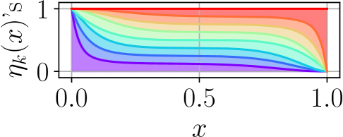
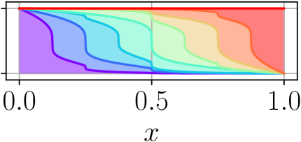
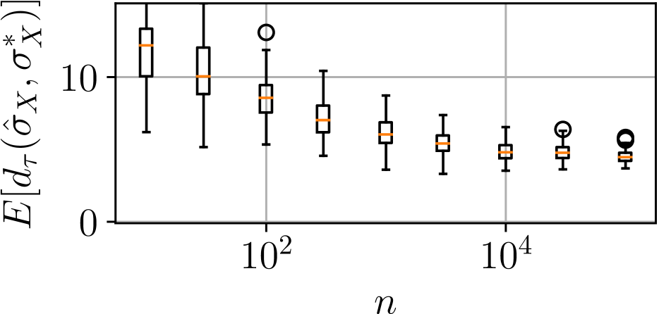
(a) $\alpha=0.2$.

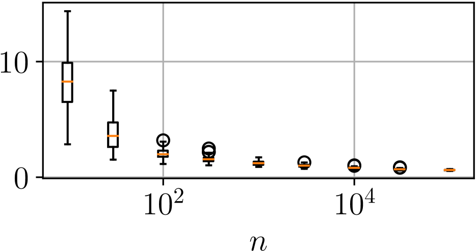
(b) $\alpha=0.8$

Figure 2: Probability of each class on $[0,1]$ for $\alpha\in\{0.2,0.8\}$ and boxplot of 100 independent estimations of $\mathbb{E}\left[d_{\tau}(\hat{\sigma}_{X},\sigma^{*}_{X})\right]$ as a function of $n$.

Real data. Regarding top-$k$ performance, for two popular datasets, MNIST and fashion-MNIST, the OVO label ranking approach is benchmarked against the rankings based on the probability estimates related to a multiclass logistic regression in Table 1.

Table 1: Top-$k$ performance. The time to fit the model is given by the last column.

Dataset	Model	Top-1	Top-5	Fit time
MNIST	LogReg	0.924	0.995	50 min
	OVO	0.943	0.997	40 min
Fashion	LogReg	0.857	0.997	35 min
-MNIST	OVO	0.863	0.997	60 min

5 CONCLUSION

In this paper, a statistical problem halfway between multiclass classification and posterior probability estimation, referred to as label ranking here, is considered. The goal is to design a method to rank, for any test observation $X$, all the labels $y$ that can be possibly assigned to it by decreasing order of magnitude of the (unknown) posterior probability $\mathbb{P}\{Y=y\mid X\}$. Formulated as a specific ranking median regression problem with incomplete observations, this problem is shown to have a solution that takes the form of a Copeland score, involving pairwise comparisons only. Based on this crucial observation, it is proved that the OVO procedure for multiclass classification permits to build, from training classification/labelled data, the optimal ranking with high probability, under appropriate hypotheses. This is also empirically supported by numerical experiments. Remarkably, the analysis carried out here incidentally provides a rate bound for the OVO classifier.

APPENDIX - TECHNICAL DETAILS

Proof of Lemma 5

As a first go, define $\Sigma^{-1}(1)$ as $Y$. Next, given $X$ and $\Sigma^{-1}(1)=Y$, draw $\Sigma^{\prime}$ as a BTLP model on the set $\mathcal{I}=\{1,\;\ldots,\;K\}\setminus\{\Sigma^{-1}(1)\}$ with preference parameters $\eta_{k}(X)$, $k\in\mathcal{I}$. For all $r\in\{1,\;\ldots,\;K-1\}$, set $\Sigma^{-1}(r+1)=\Sigma^{\prime-1}(r)$ and invert the permutation $(\Sigma^{-1}(1),\;\ldots,\;\Sigma^{-1}(K))$ to get a random permutation $\Sigma$ with the desired properties.

Proof of Theorem 10

Fix $\delta\in{0,1}$ and let $1\leq k<l\leq K$. Assumption 7 implies that the Mammen-Tsybakov noise condition is fulfilled for the binary classification problem related to the pair $(X,Y)$ given that $Y\in\{k,\;l\}$. When Assumptions 8-9 are also satisfied, a possibly fast rate bound for the risk excess of the empirical risk minimizer $\widehat{g}_{k,l}$ can be established, as stated in the following lemma.

Lemma 14

Suppose that Assumptions 7-9 are fulfilled. Let $1\leq k<l\leq K$. Then, for all $\delta\in(0,1)$, we have w.p. $\geq 1-\delta$: $\forall n\geq 1$,

$$L_{k,l}(\widehat{g}_{k,l})-L_{k,l}^{*}\leq 2\left(\inf_{g\in\mathcal{G}}L_{k,l}(g)-L_{k,l}^{*}\right)+r_{n}(\delta),$$ (16)

where, for all $n\geq n_{0}(\delta,\alpha,\epsilon,B,V)$ and $\delta\in(0,1)$,

$$r_{n}(\delta)=2\left(1/(nh)\right)^{\frac{1}{2-\alpha}}\times\\ \left[\left(64C^{2}V\log n\right)^{\frac{1}{2-\alpha}}+\left(32\log(2/\delta)\right)^{\frac{1}{2-\alpha}}\right].$$

proof.  The result is a slight variant of that proved in P. Bartlett and Mendelson (2005) (see therein), the sole difference lying in the fact that the empirical risk (and, consequently, its minimizer as well) is built from a random number of training observations (i.e. those with labels in $\{k,\;l\}$). Note that $h=\epsilon^{3-2\alpha}(1-\alpha)^{1-\alpha}\alpha^{\alpha}/B^{1-\alpha}$. Details are given in the Supplementary Material.   

Observe that the probabilities appearing in this proof are conditional probabilities given the training sample $\mathcal{D}$ and, as a consequence, must be considered as random variables. However, to simplify notations, we omit to write the conditioning w.r.t. $\mathcal{D}$ explicitly. Notice first that Assumption 7 implies that, with $\beta=B^{1-\alpha}/(\left(1-\alpha\right)^{1-\alpha}\alpha^{\alpha})$,

$$\mathbb{P}_{X}\left\{\widehat{g}_{k,l}(X)\neq g^{*}_{k,l}(X)\mid Y\in\{k,\;l\}\right\}\leq\\ \beta\left(L_{k,l}(\widehat{g}_{k,l})-L_{k,l}^{*}\right)^{\alpha},$$ (17)

with probability one. Observe in addition that

$$\mathbb{P}_{X}\left\{\widehat{g}_{k,l}(X)\neq g^{*}_{k,l}(X)\mid Y\in\{k,\;l\}\right\}=\\ \mathbb{E}_{X}\left[\frac{d\mu_{k,l}}{d\mu}(X)\times\mathbb{I}\left\{\widehat{g}_{k,l}(X)\neq g^{*}_{k,l}(X)\right\}\right],$$ (18)

denoting by $\mu_{k,l}=(p_{k}\mu_{k}+p_{l}\mu_{l})/(p_{k}+p_{l})$ the conditional distribution of $X$ given that $Y\in\{k,\;l\}$. Under Assumption 9, we almost-surely have:

$$\frac{d\mu_{k,l}}{d\mu}(X)\geq\frac{\varepsilon}{p_{k}+p_{l}}\geq\varepsilon.$$

Hence, from (17) and Lemma 14, we get that

$$\frac{\varepsilon}{\beta}\mathbb{P}_{X}\left\{\widehat{g}_{k,l}(X)\neq g^{*}_{k,l}(X)\right\}\leq\\ \left(L_{k,l}(\widehat{g}_{k,l})-L_{k,l}^{*}\right)^{\alpha}\leq 2\left(\inf_{g\in\mathcal{G}}L_{k,l}(g)-L_{k,l}^{*}\right)^{\alpha}+r_{n}^{\alpha}(\delta),$$ (19)

using Minkowski’s inequality. Since

$$\bigcap_{k<l}\left\{\widehat{g}_{k,l}(X)=g^{*}_{k,l}(X)\right\}\subset\left\{\sigma^{*}_{X}=\widehat{\sigma}_{X}\right\},$$

with probability one, combining the bound above with the union bound, for all $\delta\in(0,1)$, w.p. $\geq 1-\delta$:

$$\mathbb{P}_{X}\left\{\sigma^{*}_{X}\neq\widehat{\sigma}_{X}\right\}\leq\sum_{k<l}\mathbb{P}_{X}\left\{\widehat{g}_{k,l}(X)\neq g^{*}_{k,l}(X)\right\}\leq\\ \frac{\beta}{\varepsilon}\left\{\binom{K}{2}r_{n}^{\alpha}\left(\frac{\delta}{\binom{K}{2}}\right)+\sum_{k<l}2\left(\inf_{g\in\mathcal{G}}L_{k,l}(g)-L_{k,l}^{*}\right)^{\alpha}\right\}.$$

Proof of Proposition 12

Let us first show that $W_{k}^{*}=W_{k}(\sigma^{*}_{.}).$

For any ranking rule $s$ and all $x\in\mathbb{R}^{q}$, we define

$${\rm Top}_{k}(s(x))=\{s(X)^{-1}(1),\;\ldots,\;s(X)^{-1}(k)\},$$

and also set ${\rm Top}_{k}^{*}(x)={\rm Top}_{k}(\sigma^{*}_{x})$. Indeed, for any ranking rule $s$, we can write

$$W_{k}(s)=\mathbb{E}\left[\mathbb{E}\left[\ell_{k}(Y,\;s(X))\mid X\right]\right],$$

and we almost-surely have

$$\mathbb{E}\left[\ell_{k}(Y,\;s(X))\mid X\right]=\\ \sum_{l=1}^{K}\eta_{l}(X)\mathbb{I}\{l\notin{\rm Top}_{k}(s(X))\}.$$ (20)

As $\sigma^{*}_{x}$ is defined through (3), one easily sees that the quantity (20) is minimum for any ranking rule $s(x)$ s.t.

$${\rm Top}_{k}(s(X))={\rm Top}_{k}^{*}(X).$$ (21)

Hence, the collection of optimal ranking rules regarding the risk (15) coincides with the set of ranking rules such that (21) holds true with probability one. Observe that, with probability one,

$$\mathbb{I}\left\{Y\notin{\rm Top}_{k}(s(X))\right\}-\mathbb{I}\left\{Y\notin{\rm Top}_{k}^{*}(X)\right\}\leq\\ \mathbb{I}\left\{{\rm Top}_{k}^{*}(X)\neq{\rm Top}_{k}(s(X))\right\},$$

for any ranking rule $s(x)$, so that

$$W_{k}(s)-W^{*}_{k}\leq\mathbb{P}_{X}\left\{{\rm Top}_{k}(s(X))\neq{\rm Top}_{k}^{*}(X)\right\}.$$

In addition, notice that

$$W_{k}(\widehat{\sigma}_{X})-W_{k}^{*}\leq\mathbb{P}_{X}\left\{{\rm Top}_{k}^{*}(X)\neq{\rm Top}_{k}(\widehat{\sigma}_{X})\right\}=\\ \sum_{\mathcal{L}\subset\mathcal{Y}:\;\#\mathcal{L}=k}\mathbb{P}_{X}\left\{{\rm Top}_{k}^{*}(X)=\mathcal{L},\;{\rm Top}_{k}^{*}(X)\neq{\rm Top}_{k}(\widehat{\sigma}_{X})\right\},\\ \leq\sum_{\mathcal{L}\subset\mathcal{Y}:\;\#\mathcal{L}=k}\sum_{l\in\mathcal{L},\;m\notin\mathcal{L}}\mathbb{P}_{X}\left\{\widehat{g}_{l,m}(X)\neq g^{*}_{l,m}(X)\right\},\qquad\\ \leq\frac{\beta}{\varepsilon}\binom{K}{k}k(K-k)\times\qquad\qquad\qquad\qquad\qquad\qquad\\ \left(r_{n}^{\alpha}\left(\frac{\delta}{\binom{K}{2}}\right)+2\cdot\max_{m\neq l}\left(\inf_{g\in\mathcal{G}}L_{l,m}(g)-L_{l,m}^{*}\right)^{\alpha}\right),$$

using (19).

APPENDIX - SUPPLEMENTARY MATERIAL

5.1 Detailed proof of Lemma 14

As pointed out, the result is a slight variant of that proved in ((Boucheron et al., 2005, pages 342-346)). The sole difference lies in the fact that fact that the empirical risk (and, consequently, its minimizer as well) is built from a random number of training observations (i.e. those with labels in $\{k,\;l\}$). Here, we detail the proof for completion.

The derivation of fast learning speeds for general classes of functions relies on a sensible use of Talagrand’s inequality that exploits the upper bound on the variance of the loss provided by the noise condition, combined with convergence bounds on Rademacher averages, see P. Bartlett and Mendelson ((2005)).

To begin with, we define classes of functions that mirror the ones used by Boucheron et al. ((2005)). Those are specifically introduced for the problem of associating elements of the sample to the label $k$ or $l$, with $k<l,(k,l)\in\{1,\dots,K\}^{2}$ any pair of labels. Given a label $y\in\mathcal{Y}$, it corresponds to solving binary classification for $y_{k,l}={\mathbb{I}}\{y=k\}-{\mathbb{I}}\{y=l\}$ for all of the concerned instances, i.e. those with labels $k$ or $l$. For each binary classifier $g$ in $\mathcal{G}$, we introduce the cost function $c_{k,l}$ and the proportion of concerned instances $h_{k,l}$, such that, for all $x,y\in{\cal X}\times\{1,\dots,K\}$,

$$c_{k,l}(x,y)={\mathbb{I}}\{g(x)\neq y_{k,l},y\in\{k,l\}\}\quad\text{and}\quad h_{k,l}(y)={\mathbb{I}}\{y\in\{k,l\}\}.$$

Denote by $\mathcal{F}_{k,l}$ the regret of each function $c_{k,l}$, formally:

$$\mathcal{F}_{k,l}:=\left\{f_{k,l}:x,y\mapsto{\mathbb{I}}\{y\in\{k,l\}\}\cdot\left(c_{k,l}(x,y)-{\mathbb{I}}\{g_{k,l}^{*}(x)\neq y_{k,l}\}\right)\mid g\in\mathcal{G}\right\}.$$

With $P$ as the expectation over $X,Y$ and $P_{n}$ as the empirical measure, one can rewrite the risk $L_{k,l}$ and empirical risk $\widehat{L}_{k,l}$ as:

$$L_{k,l}(g)=\frac{Pc_{k,l}}{Ph_{k,l}}\quad\text{and}\quad\widehat{L}_{k,l}(g)=\frac{P_{n}c_{k,l}}{P_{n}h_{k,l}}.$$

Unlike $c_{k,l}$ the empirical mean $P_{n}h_{k,l}$ does not depend on an element of $g\in\mathcal{G}$, thus minimizing $\widehat{L}_{k,l}$ is the same problem as minimizing $P_{n}c_{k,l}$. The rest of the proof consists in using ((Boucheron et al., 2005, section 5.3.5 therein)) to derive an upper bound of $Pf$, with $f\in\mathcal{F}_{k,l}$. Talagrand’s inequality is useful because of an upper-bound on the variance of the elements in $\mathcal{F}_{k,l}$.

Assumption 7 induces a control on the variance of the elements of $\mathcal{F}_{k,l}$. ((Bousquet et al., 2004, page 202 therein)) reviewed equivalent formulations of the noise assumption, in the case of binary classification. One of those formulations is similar to the following equation:

$$\mathbb{P}\left\{g(X)\neq g^{*}_{k,l}(X)\right\}\leq\beta(L_{k,l}(g)-L_{k,l}^{*})^{\alpha},$$ (22)

where $\beta=\frac{B^{1-\alpha}}{\epsilon(1-\alpha)^{1-\alpha}\alpha^{\alpha}}$. The proof is the same as that of ((Bousquet et al., 2004, page 202 therein)), but is followed by Assumption 9, see section 5.1.1 for more details.

Set $\beta_{0}=\beta(p_{k}+p_{l})^{\alpha}$, Equation (22) implies, for any $f\in\mathcal{F}_{k,l}$, that, with $T(f)=\sqrt{\beta_{0}}\cdot(Pf)^{\alpha/2}$:

$$\text{Var}(f)\leq\mathbb{P}\left\{g(X)\neq g^{*}_{k,l}(X)\right\}\leq\beta(L_{k,l}(g)-L_{k,l}^{*})^{\alpha}=\beta(p_{k}+p_{l})^{\alpha}\cdot(Pf)^{\alpha}=T^{2}(f).$$ (23)

The function $T(f)$ controls the variance of the elements in $\mathcal{F}_{k,l}$, and is used to reweights its instances before applying Talagrand’s inequality.

The complexity of the proposal family of functions is controlled using the notion of Rademacher average, as in Boucheron et al. ((2005)). Let $\mathcal{F}$ be a class of functions, its Rademacher average $R_{n}(\mathcal{F})$ is defined as:

$$R_{n}(\mathcal{F}):=\mathbb{E}_{\sigma}\sup_{f\in\mathcal{F}}\frac{1}{n}\left\lvert\sum_{i=1}^{n}\sigma_{i}f(X_{i},Y_{i})\right\rvert.$$

Introduce $\mathcal{F}_{k,l}^{*}$ as the star-hull of $\mathcal{F}_{k,l}$, i.e. $\mathcal{F}_{k,l}^{*}=\{\alpha f:\alpha\in[0,1],f\in\mathcal{F}_{k,l}\}$, we define two functions that characterize the properties of the problem of interest, and are required to apply ((Boucheron et al., 2005, Theorem 5.8 therein)):

$$w(r)=\sup_{f\in\mathcal{F}_{k,l}^{*}:Pf\leq r}T(f)\qquad\text{ and }\qquad\psi(r)=\mathbb{E}R_{n}\{f\in\mathcal{F}_{k,l}^{*}:T(f)\leq r\}.$$ (24)

Finally ((Boucheron et al., 2005, Theorem 5.8 therein)) implies that, for all $\delta>0$, with $r^{*}_{0}(\delta)$ the solution of:

$$r=4\psi(w(r))+2w(r)\sqrt{\frac{2\log\frac{2}{\delta}}{n}}+\frac{16\log\frac{2}{\delta}}{3n},$$ (25)

we have that, with probability at least $1-\delta$,

$$L_{k,l}(\hat{g}_{k,l})-L_{k,l}^{*}\leq 2\left(\inf_{g\in\mathcal{G}}L_{k,l}(g)-L_{k,l}^{*}\right)+\frac{r_{0}^{*}(\delta)}{p_{k}+p_{l}}.$$

Now, we can conclude by combining this result with properties of $w$ and $\psi$, that originate from the noise assumption and the control on the complexity of $\mathcal{G}$, respectively. Assumption 8 states that the proposal class $\mathcal{G}$ is of VC-dimension $V$. Permanence properties of VC-classes of functions, see ((van der Vaart and Wellner, 1996, section 2.6.5 therein)), imply that $\mathcal{F}_{k,l}$ is also VC. It follows from P. Bartlett and Mendelson ((2005)) that:

$$\psi(r)\leq Cr\sqrt{\frac{V}{n}\log n}.$$

Plugging this result into Equation 25 gives:

$$r^{*}_{0}(\delta)\leq\frac{2w(r^{*}_{0}(\delta))}{\sqrt{n}}\left[2C\sqrt{V\log n},+\sqrt{2\log\frac{2}{\delta}}\right]+\frac{16\log\frac{2}{\delta}}{3n}.$$

Combining it with the definition of $w$ in (24) and the control on the variance laid forth in (23) yields:

$$r^{*}_{0}(\delta)\leq\left[r^{*}_{0}(\delta)\right]^{\alpha/2}\frac{2\sqrt{\beta_{0}}}{\sqrt{n}}\left[2C\sqrt{V\log n}+\sqrt{2\log\frac{2}{\delta}}\right]+\frac{16\log\frac{2}{\delta}}{3n}.$$ (26)

Equation (26) is a variational inequality, and an upper bound on the solution can be derived directly from ((Zou et al., 2009, Lemma 2 therein)). It writes:

$$r^{*}_{0}(\delta)\leq\max\left\{\left(\frac{16\beta_{0}}{n}\right)^{\frac{1}{2-\alpha}}\left[2C\sqrt{V\log n}+\sqrt{2\log(2/\delta)}\right]^{\frac{2}{2-\alpha}},\frac{32\log(2/\delta)}{3n}\right\}.$$

Using the convexity of $x\mapsto x^{\frac{2}{2-\alpha}}$, the right-hand side of the above inequality can be upper-bounded, which leads to:

$$r^{*}_{0}(\delta)\leq 2\cdot\max\left\{\left(\frac{16\beta_{0}}{n}\right)^{\frac{1}{2-\alpha}}\left[\left(4C^{2}V\log n\right)^{\frac{1}{2-\alpha}}+\left(2\log(2/\delta)\right)^{\frac{1}{2-\alpha}}\right],\frac{32\log(2/\delta)}{3n}\right\}.$$ (27)

Assumption 9 implies that $(p_{k}+p_{l})^{-1}\leq 1/\epsilon$. Introducing $r^{*}(\delta)=(p_{k}+p_{l})^{-1}r_{0}^{*}(\delta)$, Equation (27) combined with the definition of $\beta_{0}$ implies:

$$r^{*}(\delta)\leq 2\cdot\max\left\{\left(\frac{16\beta}{\epsilon^{2-2\alpha}n}\right)^{\frac{1}{2-\alpha}}\left[\left(4C^{2}V\log n\right)^{\frac{1}{2-\alpha}}+\left(2\log(2/\delta)\right)^{\frac{1}{2-\alpha}}\right],\frac{32\log(2/\delta)}{3\epsilon n}\right\}.$$ (28)

Introduce $n_{0}(\delta,\alpha,\epsilon,B,V)$ as the lowest $n$ such that the first term in the maximum in Equation (28) dominates the second term, it satisfies:

$$n_{0}^{\frac{1-\alpha}{2-\alpha}}\left[\left(4C^{2}V\log(n_{0})\right)^{\frac{1}{2-\alpha}}+\left(2\log(2/\delta)\right)^{\frac{1}{2-\alpha}}\right]\geq\frac{32\log(2/\delta)}{3\left[16\beta\epsilon^{\alpha}\right]^{\frac{1}{2-\alpha}}}.$$ (29)

and so does any $n\geq n_{0}$.

To conclude, we have proven that for any $\delta\in(0,1)$, for any $n\geq n_{0}(\delta,\alpha,\epsilon,B,V)$, we have that, with probability greater than $1-\delta$,

$$L_{k,l}(\hat{g}_{k,l})-L_{k,l}^{*}\leq 2\left(\inf_{g\in\mathcal{G}}L_{k,l}(g)-L_{k,l}^{*}\right)+r^{*}(\delta),$$

with

$$r^{*}(\delta)=2\left(\frac{16\beta}{n\epsilon^{2-2\alpha}}\right)^{\frac{1}{2-\alpha}}\left[\left(4C^{2}V\log n\right)^{\frac{1}{2-\alpha}}+\left(2\log(2/\delta)\right)^{\frac{1}{2-\alpha}}\right].$$ (30)

A simple upper bound on $n_{0}(\delta,\alpha,\epsilon,B,V)$:

The right-side terms of Equation (30) are not balanced. Indeed, as soon as $n$ is high, the term in $\log(n)$ dominates the other. That fact can be exploited to derive a convenient upper bound on $n_{0}(\delta,\alpha,\epsilon,B,V)$, since one cannot directly solve eq. 29.

Assume that $n\geq(2/\delta)^{\frac{1}{2C^{2}V}}$, then

$$n^{\frac{1-\alpha}{2-\alpha}}\left[\left(4C^{2}V\log(n)\right)^{\frac{1}{2-\alpha}}+\left(2\log(2/\delta)\right)^{\frac{1}{2-\alpha}}\right]\geq 2\left(2n^{1-\alpha}\log(2/\delta)\right)^{\frac{1}{2-\alpha}}.$$

However, we have that:

$$2\left(2n^{1-\alpha}\log(2/\delta)\right)^{\frac{1}{2-\alpha}}\geq\frac{32\log(2/\delta)}{3\left[16\beta\epsilon^{\alpha}\right]^{\frac{1}{2-\alpha}}},$$

if and only if:

$$n\geq\log(2/\delta)\left(\frac{(16/3)^{2-\alpha}}{32\beta\epsilon^{\alpha}}\right)^{\frac{1}{1-\alpha}}.$$

Hence, we have proven that:

$$n_{0}(\delta,\alpha,\epsilon,B,V)\leq\max\left\{(2/\delta)^{\frac{1}{2C^{2}V}},\log(2/\delta)\left(\frac{(16/3)^{2-\alpha}}{32\beta\epsilon^{\alpha}}\right)^{\frac{1}{1-\alpha}}\right\}.$$

5.1.1 On the equivalent noise condition

The proof is almost similar to that of ((Bousquet et al., 2004, page 202 therein)), and is recalled here. The excess loss of a classifier can be written as follows:

$$L_{k,l}(g)-L^{*}_{k,l} =\mathbb{E}\left[\left\lvert 2\eta_{k,l}(X)-1\right\rvert\cdot{\mathbb{I}}\left\{g(X)\neq g_{k,l}^{*}(X)\right\}\mid Y\in\left\{k,l\right\}\right].$$

Using Markov’s inequality, for all $t\geq 0$:

$$L_{k,l}(g)-L_{k,l}^{*} \geq t\cdot\mathbb{E}\left[{\mathbb{I}}\left\{g(X)\neq g_{k,l}^{*}(X)\right\}\cdot{\mathbb{I}}\left\{\left\lvert 2\eta_{k,l}(X)-1\right\rvert\geq t\right\}\mid Y\in\left\{k,l\right\}\right],$$

$$\geq t\cdot{\mathbb{P}}\left\{\left\lvert 2\eta_{k,l}(X)-1\right\rvert\geq t\mid Y\in\left\{k,l\right\}\right\}$$

$$\qquad\qquad-t\cdot\mathbb{E}\left[{\mathbb{I}}\left\{g(X)=g^{*}_{k,l}(X)\right\}{\mathbb{I}}\left\{\left\lvert 2\eta_{k,l}(X)-1\right\rvert\geq t\right\}\mid Y\in\left\{k,l\right\}\right].$$

Assumption 7 and ${\mathbb{I}}\left\{\left\lvert 2\eta_{k,l}(X)-1\right\rvert\geq t\right\}\leq 1$ imply:

$$L_{k,l}(g)-L_{k,l}^{*} \geq t\cdot(1-Bt^{\frac{\alpha}{1-\alpha}})-t\cdot{\mathbb{P}}\left\{g(X)=g_{k,l}^{*}(X)\mid Y\in\left\{k,l\right\}\right\}$$

$$\geq t\cdot\left({\mathbb{P}}\left\{g(X)\neq g_{k,l}^{*}(X)\mid Y\in\left\{k,l\right\}\right\}-Bt^{\frac{\alpha}{1-\alpha}}\right),$$

Choosing

$$t=\left[\frac{(1-\alpha){\mathbb{P}}\left\{g(X)\neq g_{k,l}^{*}(X)\mid Y\in\left\{k,l\right\}\right\}}{B}\right]^{(1-\alpha)/\alpha},$$

finally gives:

$${\mathbb{P}}\left\{g(X)\neq g_{k,l}^{*}(X)\mid Y\in\left\{k,l\right\}\right\}\leq\frac{B^{1-\alpha}}{(1-\alpha)^{1-\alpha}\alpha^{\alpha}}(L_{k,l}(g)-L_{k,l}^{*})^{\alpha}.$$

Which implies, using Assumption 9:

$${\mathbb{P}}\left\{g(X)\neq g_{k,l}^{*}(X)\right\}\leq\frac{B^{1-\alpha}}{\epsilon(1-\alpha)^{1-\alpha}\alpha^{\alpha}}(L_{k,l}(g)-L_{k,l}^{*})^{\alpha}.$$

5.2 Experiments on simulated data

Introduce the function $h_{\alpha}$, which for any $\alpha\in[0,1]$:

$$h_{\alpha}(x)=\frac{1}{2}+\frac{1}{2}\epsilon(x)\left\lvert 2x-1\right\rvert^{\frac{1-\alpha}{\alpha}},$$

where $\epsilon(x)=2{\mathbb{I}}\left\{2x>1\right\}-1$. It has good properties with regard to the Mammen-Tsybakov noise condition introduced in Boucheron et al. ((2005)). We define a warped version $h_{\alpha,x_{0}}$ of this function $h_{\alpha}$ such that:

$$h_{\alpha,x_{0}}(x)=\begin{cases}h_{\alpha,x_{0}}=h_{\alpha}\left(\frac{x}{2x_{0}}\right)&\text{if }x<x_{0},\\ h_{\alpha,x_{0}}=h_{\alpha}\left(\frac{1}{2}+\frac{x-x_{0}}{2(1-x_{0})}\right)&\text{if }x\geq x_{0}.\\ \end{cases}$$

We use this function to define the $\eta_{k}$’s by recursion, and assume that $X\sim\mathcal{U}([0,1])$. Formally, define a depth parameter $D$, the variable $Y$ belong to $K=2^{D+1}$ classes. Let $b_{2}^{(d)}(k)$ describe the decomposition in base 2 of the value $k$, i.e. $k=\sum_{d=0}^{D}2^{b_{2}^{(d)}(k)}$, we set, with $x_{(d,k)}=\sum_{d=1}^{D}2^{-b_{2}^{(d)}(k)}$:

$$\eta_{k}(x)=\prod_{d=0}^{D}h_{\alpha,x_{(d,k)}}(x).$$

By varying the parameter $\alpha$, one can set the classification problems to be more complicated or more easy. If $\alpha$ is close to $1$, the problems are very simple. If $\alpha$ is close to $0$, the problems are more arduous.

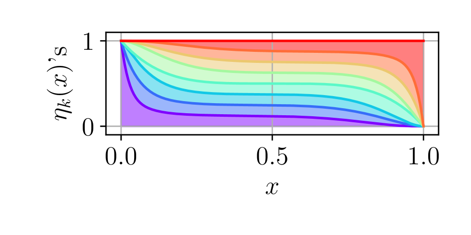
(a) Distribution for $\alpha=0.2$.

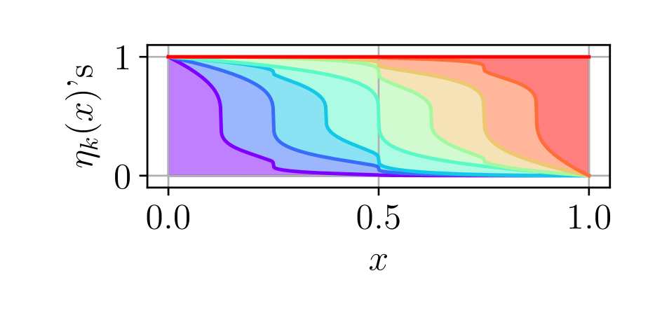
(b) Distribution for $\alpha=0.8$.

Figure 3: Cumulated histogram of the $\eta_{k}$’s over $[0,1]$.

To implement the procedure described in Figure 1, we learn decision stumps in $[0,1]$, i.e. we optimize over the family of functions $\mathcal{G}=\left\{g_{s,\epsilon}\mid s\in[0,1],\epsilon\in\{-1,+1\}\right\}$, where, for any $x\in[0,1]$:

$$g_{s,\epsilon}(x)=2{\mathbb{I}}\left\{(x-s)\epsilon\geq 0\right\}-1.$$

Figure 6, Figure 6 and Figure 6 represent boxplots obtained with 100 independent estimations on 1000 test points of, respectively, the number of cycles in predicted permutations, the average miss probability for the problem of predicting permutations $\mathbb{P}\{\hat{\sigma}_{X}\neq\sigma_{X}^{*}\}$, and the average Kendall distances between predictions and ground truths $\mathbb{E}\left[d_{\tau}(\hat{\sigma}_{X},\sigma_{X}^{*})\right]$, all as a function of the number of learning points $n$ with

$$n\in\bigcup_{i\in[\![1,4]\!]}\{10^{i},3\times 10^{i}\}\cup\{10^{5}\}.$$

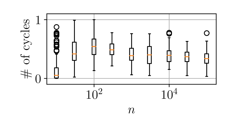
(a) Dynamics for $\alpha=0.2$.

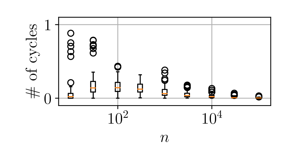
(b) Dynamics for $\alpha=0.8$

Figure 4: Boxplot of 100 independent estimations of the proportion of predictions with cycles as a function of $n$.

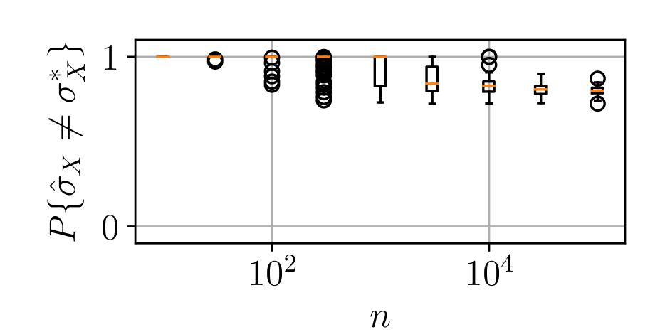
(c) Dynamics for $\alpha=0.2$.

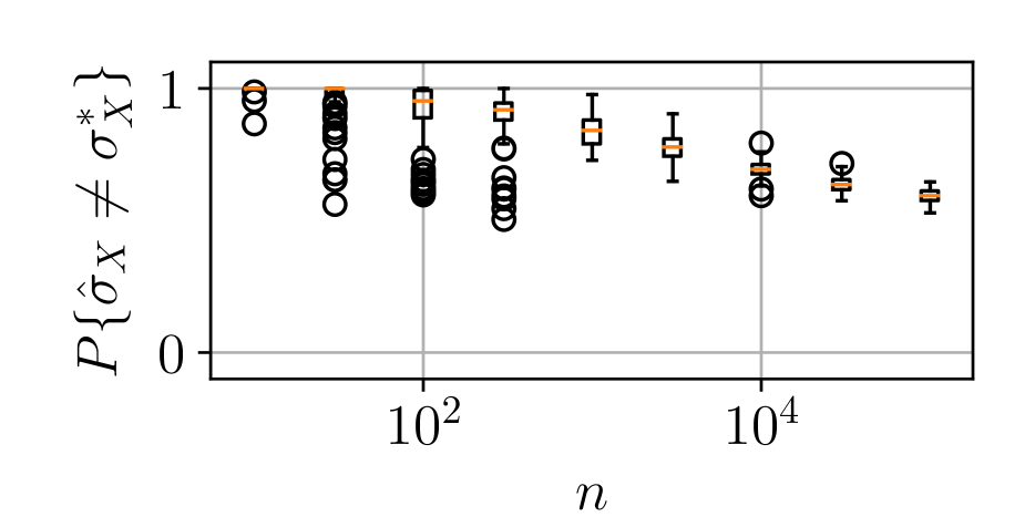
(d) Dynamics for $\alpha=0.8$

Figure 5: Boxplot of 100 independent estimations of $\mathbb{P}\{\widehat{\sigma}_{X}\neq\sigma^{*}_{X}\}$ as function of $n$.

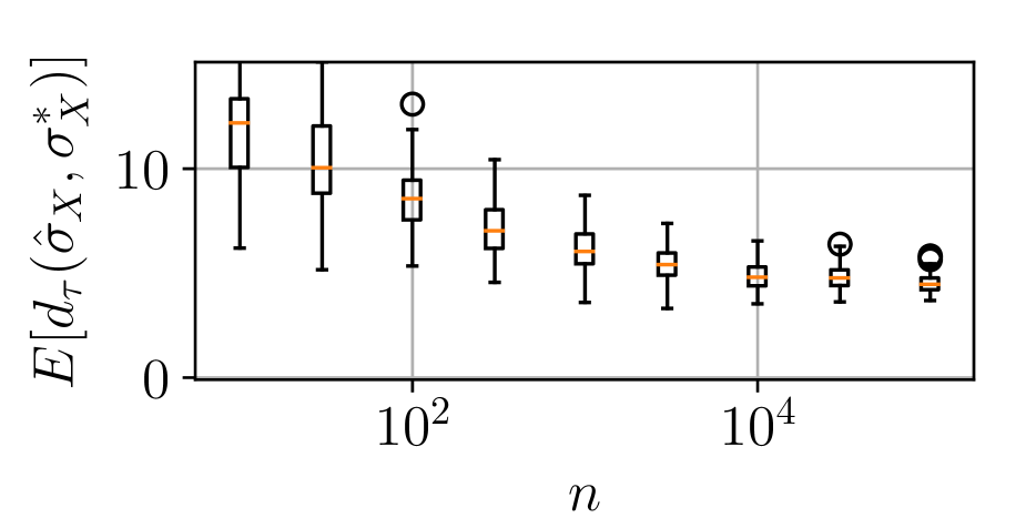
(a) Dynamics for $\alpha=0.2$.

(b) Dynamics for $\alpha=0.8$

Figure 6: Boxplot of 100 independent estimations of $\mathbb{E}\left[d_{\tau}(\hat{\sigma}_{X},\sigma_{X}^{*})\right]$ as function of $n$.

One sees that learning is fast when $\alpha$ is close to 1, as expected. Figure 6 shows that the average Kendall’s $\tau$ distance decreases quickly when $\alpha$ is close to $1$, as does the the proportion of cycle in predictions, see Figure 6. On the other hand, due to the difficulty of predicting a complete permutation, the influence of the noise parameter on the evolution of the probability of error when $n$ grows is more subtle, see Figure 6.

5.3 Experiments on real data

The MNIST dataset is composed of $28\times 28$ grayscale images of digits and labels being the value of the digits. In this experiment, we learn to predict the value of the digit between $K=10$ classes corresponding to digits between $0$ and $9$. The dataset contains $60,000$ images for training and $10,000$ images for testing, all equally distributed within the classes. This dataset has been praised for its accessibility, but was recently criticised for being too easy, which led to the introduction of the dataset Fashion-MNIST, see Xiao et al. ((2017)). It has the same structure as MNIST, with regard to train and test splits, number of classes and and image size. It consists in classifying types of clothing apparel, e.g. dress, coat and sandals, and is harder to classify than MNIST.

Our experiments aim to show that the OVO approach for top-$k$ classification, cf Eq. (15), can surpass rankings relying on the scores output by multiclass classification algorithms. For that matter, we evaluated the performances of both approaches using a logistic regression to solve binary classification in the OVO case and multiclass classification in the other. For that matter, we relied on the implementations provided by the python package scikit-learn, specifically the LogisticRegressionCV class. The dimensionality of the data was reduced using standard PCA with enough components to retain 95% of the variance for both datasets, which makes for $153$ components for MNIST and $187$ components for Fashion-MNIST.

Results are summarized in Table 1. They show that the OVO approach performs better than the logistic regression for the top-$1$ accuracy, i.e. classification accuracy, as well as for the top-$5$ accuracy. While the OVO approach requires us to train $K(K-1)/2=45$ models, those are trained with less data and output values. Both approaches end up requiring a similar amount of time to be trained.

References

- Allwein et al. (2000) E. Allwein, R. Schapire, and Y. Singer. Reducing multiclass to binary: a unifying approach for margin classifiers. Journal of Machine Learning Research, 1:113–141, 2000.
- Boucheron et al. (2005) S. Boucheron, O. Bousquet, and G. Lugosi. Theory of classification : a survey of some recent advances. ESAIM: Probability and Statistics, 9:323–375, 2005.
- Bousquet et al. (2004) O. Bousquet, S. Boucheron, and G. Lugosi. Introduction to statistical learning theory. In Advanced Lectures on Machine Learning, pages 169–207. 2004.
- Bradley and Terry (1952) R. A. Bradley and M. E. Terry. Rank analysis of incomplete block designs: I. the method of paired comparisons. Biometrika, 39(3/4):324–345, 1952.
- Brinker and Hüllermeier (2019) K. Brinker and E. Hüllermeier. A reduction of label ranking to multiclass classification. In ECML PKDD. 2019.
- Clémençon et al. (2018) S. Clémençon, A. Korba, and E. Sibony. Ranking median regression: Learning to order through local consensus. In Proceedings of the conference Algorithmic Learning Theory, 2018.
- Copeland (1951) A. H. Copeland. A reasonable social welfare function. In Seminar on applications of mathematics to social sciences, University of Michigan, 1951.
- Devroye et al. (1996) L. Devroye, L. Györfi, and G. Lugosi. A probabilistic theory of pattern recognition. Springer, 1996.
- Deza and Huang (1998) M. Deza and T. Huang. Metrics on permutations, a survey. 1998.
- Di Battista et al. (1999) G. Di Battista, P. Eades, R. Tamasia, and I. Tollis. Graph Drawing. Prentice Hall, 1999.
- Festa et al. (1999) P. Festa, P. Pardalos, and M. C. Resende. Feedback Set Problems, pages 209–258. Springer US, Boston, MA, 1999.
- Fürnkranz (2002) J. Fürnkranz. Round robin classification. Journal of Machine Learning Research, 2:721–747, 2002.
- Hastie and Tibshirani (1998) T. Hastie and R. Tibshirani. Classification by pairwise coupling. In Proceedings of NIPS, 1998.
- Korba et al. (2017) A. Korba, S. Clémençon, and E. Sibony. A learning theory of ranking aggregation. In Proceeding of AISTATS 2017, 2017.
- Korba et al. (2018) A. Korba, A. Garcia, and F. d’Alché Buc. A structured prediction approach for label ranking. In NeurIPS. 2018.
- Luce (1959) R. D. Luce. Individual Choice Behavior. Wiley, 1959.
- Mammen and Tsybakov (1999) E. Mammen and A. Tsybakov. Smooth discrimination analysis. The Annals of Statistics, 27(6):1808–1829, 1999.
- Massart and Nédélec (2006) P. Massart and E. Nédélec. Risk bounds for statistical learning. Annals of Statistics, 34(5), 2006.
- Moreira and Mayoraz (1998) M. Moreira and E. Mayoraz. Improved pairwise coupling classification with correcting classifiers. In In the Proceedings of ECML, 1998.
- P. Bartlett and Mendelson (2005) O. B. P. Bartlett and S. Mendelson. Localized rademacher complexities. The Annals of Statistics, 33(1):497–1537, 2005.
- Plackett (1975) R. L. Plackett. The analysis of permutations. Applied Statistics, 2(24):193–202, 1975.
- Tsoumakas et al. (2009) G. Tsoumakas, I. Katakis, and I. Vlahavas. Mining multi-label data. In Data mining and knowledge discovery handbook, pages 667–685. Springer, 2009.
- van der Vaart and Wellner (1996) A. van der Vaart and J. A. Wellner. Weak convergence and empirical processes. 1996. ISBN 0-387-94640-3. doi: 10.1007/978-1-4757-2545-2.
- Vapnik (1998) V. Vapnik. Statistical Learning Theory. Wiley, New York, 1998.
- Vembu and Gärtner (2010) S. Vembu and T. Gärtner. Label ranking algorithms: A survey. In Preference learning, pages 45–64. Springer, 2010.
- Weston and Watkins (1999) J. Weston and C. Watkins. Multiclass support vector machines. In Proceedings of ESANN99, D. Facto Press, Brussels., 1999.
- Wu et al. (2004) T. Wu, C. Lin, and R. Weng. Probability estimates for multi-class classification by pairwise coupling. Journal of Machine Learning Research, 5:975–1005, 2004.
- Xiao et al. (2017) H. Xiao, K. Rasul, and R. Vollgraf. Fashion-mnist: a novel image dataset for benchmarking machine learning algorithms. CoRR, abs/1708.07747, 2017. URL http://arxiv.org/abs/1708.07747.
- Zou et al. (2009) B. Zou, H. Zhang, and Z. Xu. Learning from uniformly ergodic Markov chains, volume 25. 2009.