Recursive, parameter-free, explicitly defined interpolation nodes for simplices

Abstract

A rule for constructing interpolation nodes for $n$th degree polynomials on the simplex is presented. These nodes are simple to define recursively from families of 1D node sets, such as the Lobatto-Gauss-Legendre (LGL) nodes. The resulting nodes have attractive properties: they are fully symmetric, they match the 1D family used in construction on the edges of the simplex, and the nodes constructed for the $(d-1)$-simplex are the boundary traces of the nodes constructed for the $d$-simplex. When compared using the Lebesgue constant to other explicit rules for defining interpolation nodes, the nodes recursively constructed from LGL nodes are nearly as good as the warp & blend nodes of [War06] in 2D (which, though defined differently, are very similar), and in 3D are better than other known explicit rules by increasing margins for $n>6$. By that same measure, these recursively defined nodes are not as good as implicitly defined nodes found by optimizing the Lebesgue constant or related functions, but such optimal node sets have yet to be computed for the tetrahedron. A reference python implementation has been distributed as the recursivenodes package, but the simplicity of the recursive construction makes them easy to implement.

1 Definition of the recursive rule

The motivating example for this work is the use of Lagrange polynomials as shape functions for the finite element approximation space $\mathcal{P}_{n}(\Delta^{d})$: polynomials of degree at most $n$ on the $d$-simplex. A Lagrange polynomial basis $\Phi_{X}=\{\varphi_{i}\}\subset\mathcal{P}_{n}(\Delta^{d})$ is defined by a set of interpolation nodes $X=\{\boldsymbol{x}_{i}\}\subset\Delta^{d}$ as $\Phi_{X}=\{\varphi_{i}\in\mathcal{P}_{n}(\Delta^{d}):\varphi_{i}(\boldsymbol{x}_{j})=\delta_{ij}\}$. While some of the properties of an implementation of the finite element method depend only on the approximation space, the basis used, whether Lagrange or other, can affect the convergence, numerical stability, and computational efficiency of the method. Convergence is affected by the way the basis is used to approximate data, numerical stability by presence of round-off errors, in the construction of both the basis and the resulting systems of equations, and computational efficiency by the complexity of common tasks like applying a mass or derivative matrix. Discussion of each of these aspects follows the definition of the interpolation nodes that are the main contribution of this work.

The nodes are dimensionally recursive, building from points on the interval $[0,1]$. A 1D node set is a set of points $X_{n}=\{x_{n,i}\}_{i=0}^{n}\subset[0,1]$ that is increasing and symmetric about $1/2$, $x_{n,i}=1-x_{n,n-i}$. A 1D node family is a collection $\boldsymbol{X}=\{X_{n}\}_{n\in\mathbb{N}_{0}}$. Examples include equispaced nodes, symmetric Gauss-Jacobi quadrature nodes, and symmetric Lobatto-Gauss-Jacobi quadrature nodes.

The new nodes are naturally defined on the barycentric $d$-simplex,

$$\Delta^{d}_{\text{bary}}=\{\boldsymbol{b}=(b_{0},\dots,b_{d})\in\mathbb{R}^{d+1}_{+}:{\textstyle\sum_{i}}\,b_{i}=1\},$$

and are naturally indexed by the multi-indices

$$A^{d}_{n}=\{\boldsymbol{\alpha}=(\alpha_{0},\dots,\alpha_{d})\in\mathbb{N}_{0}^{d+1}:|\boldsymbol{\alpha}|=n\}.$$

This work uses the standard notation $|\boldsymbol{\alpha}|=\sum_{i}\alpha_{i}$, and further defines:

• $\#\boldsymbol{x}$ as the length of a tuple (multi-index or vector),

• $\boldsymbol{x}_{\backslash i}$ as the tuple formed by removing the $i$th element, and

• $\boldsymbol{x}_{+i}$ as the augmentation of a tuple by inserting a zero for the $i$th element.

Given a 1D node family $\boldsymbol{X}$, the recursive definition of the interpolation node $\boldsymbol{b}_{\boldsymbol{X}}(\boldsymbol{\alpha})\in\Delta^{\#\boldsymbol{\alpha}-1}_{\text{bary}}$ is

$$\boldsymbol{b}_{\boldsymbol{X}}(\boldsymbol{\alpha})=\begin{cases}(1),&\#\boldsymbol{\alpha}=1,\\ \frac{\displaystyle{\textstyle\sum_{i}}\,x_{|\boldsymbol{\alpha}|,|\boldsymbol{\alpha}_{\backslash i}|}\boldsymbol{b}_{\boldsymbol{X}}(\boldsymbol{\alpha}_{\backslash i})_{+i}}{\displaystyle{\textstyle\sum_{i}}\,x_{|\boldsymbol{\alpha}|,|\boldsymbol{\alpha}_{\backslash i}|}},&\#\boldsymbol{\alpha}>1.\end{cases}$$ (1)

The full $d$-simplex node set is

$$R^{d}_{\boldsymbol{X},n}=\{\boldsymbol{b}_{\boldsymbol{X}}(\boldsymbol{\alpha}):\boldsymbol{\alpha}\in A^{d}_{n}\},$$ (2)

and the full $d$-simplex node family is

$$\boldsymbol{R}^{d}_{\boldsymbol{X}}=\{R^{d}_{\boldsymbol{X},n}\}_{n\in\mathbb{N}}.$$ (3)

Unless otherwise specified, the 1D node family $\boldsymbol{X}$ is taken to be the Lobatto-Gauss-Legendre (LGL) family $\boldsymbol{X}_{\text{LGL}}$. Some examples are illustrated in Fig. 1.

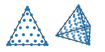
Figure 1: The nodes $R^{2}_{\boldsymbol{X},7}$ and $R^{3}_{\boldsymbol{X},7}$, mapped to equilateral simplices.

2 Intuition behind the recursive rule

[BP06] observed that Fekete points for the triangle, which have good interpolation properties, points in the interior nearly project onto LGL nodes on the edges of the triangle:

Some intriguing observations can be made regarding the location of some of the Fekete points in a given set. […] If an imaginary line is drawn through the nodes […] the two Fekete nodes sit on this line, close to the two zeros of the second Lobatto polynomial, Lo2, scaled by the length of the imaginary line.

From this comes the idea that, if a good family of interpolation nodes on the $(d-1)$-simplex are already known, a heuristic for locating the node $\boldsymbol{b}_{\boldsymbol{X}}(\boldsymbol{\alpha})$ in the $d$-simplex is to choose a point whose projection onto each facet from the opposite vertex is one of those good nodes,

$$\frac{\boldsymbol{b}_{\boldsymbol{X}}(\boldsymbol{\alpha})_{\backslash i}}{1-b_{\boldsymbol{X},i}(\boldsymbol{\alpha})}=\boldsymbol{b}_{\boldsymbol{X}}(\boldsymbol{\alpha}_{\backslash i}),\quad\forall\ i\in\{0,\dots,d\}.$$ (4)

Unfortunately, this is an overdetermined set of requirements.

Consider for example the placement of the interpolation node with multi-index $\boldsymbol{\alpha}=(1,2,3)$ in the barycentric triangle (this is one of the nodes for $n=|\boldsymbol{\alpha}|=6$). The LGL nodes are good interpolation nodes, so the desire is for $\boldsymbol{b}_{\boldsymbol{X}}((1,2,3))$ to project onto the LGL nodes associated with the multi-indices $(2,3)$ (one of the nodes for $n=2+3=5$), $(1,3)$ ($n=4$), and $(1,2)$ ($n=3$), as illustrated in Fig. 2 (right). The projection lines nearly intersect at one point, but not quite. The system (4) has a solution if $\boldsymbol{X}$ is the family of equispaced nodes, and the solution is an equispaced node in the triangle, as seen in Fig. 2 (left).

Figure 2: Desired projections for $\boldsymbol{b}_{\boldsymbol{X}}((1,2,3))$. If $\boldsymbol{X}$ is the equispaced 1D node family (left), the projections meet at an equispaced node in the triangle. If $\boldsymbol{X}$ is the LGL 1D node family (right), the lines do not actually meet at one point (detail, 32x magnified).

Any point in the interior of the triangle is in the convex hull of its projections onto the edges, so if a node location does satisfy (4), then it can be expressed as a barycentric combination of its projections. The equispaced nodes of the triangle not only have projections that are equispaced nodes on the edges, but their barycentric weights have a remarkable property.

Proposition 2.1.

Let the barycentric coordinates of the equispaced node associated with $\boldsymbol{\alpha}=(\alpha_{0},\alpha_{1},\alpha_{2})$, $|\boldsymbol{\alpha}|=n$, be $\boldsymbol{b}=(\alpha_{0}/n,\alpha_{1}/n,\alpha_{2}/n)$. Let its projections onto the edges be

$$\boldsymbol{b}_{0} =(0,\alpha_{1}/(n-\alpha_{0}),\alpha_{2}/(n-\alpha_{0})),$$

$$\boldsymbol{b}_{1} =(\alpha_{0}/(n-\alpha_{1}),0,\alpha_{2}/(n-\alpha_{1})),$$

$$\boldsymbol{b}_{2} =(\alpha_{0}/(n-\alpha_{2}),\alpha_{1}/(n-\alpha_{2}),0).$$

Then $\boldsymbol{b}$ is a convex combination of $\boldsymbol{b}_{0}$, $\boldsymbol{b}_{1}$, and $\boldsymbol{b}_{2}$ with (unnormalized) barycentric weights $(1-\alpha_{0}/n):(1-\alpha_{1}/n):(1-\alpha_{2}/n)$.

In Proposition 2.1, the barycentric weights describing equispaced nodes in the triangle are themselves 1D equispaced nodes on the edge (see Fig. 3, left). By analogy, a heuristic for approximating a solution to the overdetermined system (4) is to use the same 1D node family $\boldsymbol{X}$ that was used for the projection points as barycentric weights for combining them (see Fig. 3, right), which restates (1).

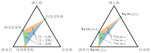
Figure 3: Defining $\boldsymbol{b}_{\boldsymbol{X}}((1,2,3))$ by barycentric coordinates relative to the projection points. If $\boldsymbol{X}$ is the equispaced 1D node family (left), it is the same as the point as the intersection of projection lines (see Fig. 2). If $\boldsymbol{X}$ is an arbitrary 1D node family (right), it is the recursive rule (1).

3 Comparison to other node families

The recursive rule (1) generates node families $\boldsymbol{R}^{d}_{\boldsymbol{X}}$ for the $d$-simplex in each dimension. This section compares them to other node families with respect to several metrics that are relevant to finite element computations.

3.1 Boundary and symmetry properties

The nodes $R^{d}_{\boldsymbol{X},n}$ have three non-numerical properties that make them convenient to use when implementing the finite element method.

1. Symmetry: The symmetry group of the $d$-simplex is the group $S_{d+1}$: for $\Delta^{d}_{\text{bary}}$, each symmetry corresponds to a permutation of the coordinates. It is clear that the recursive rule (1) respects these symmetries, that $\boldsymbol{b}_{\boldsymbol{X}}(\sigma(\boldsymbol{\alpha}))=\sigma(\boldsymbol{b}_{\boldsymbol{X}}(\boldsymbol{\alpha}))$. This is useful when a $d$-simplex is viewed from multiple orientations, such as when it is the interface between cells.

2. Equivalence to $\boldsymbol{X}$ when $d=1$: The node sets in $\boldsymbol{X}$ must be symmetric about $1/2$, so if $\boldsymbol{\alpha}=(\alpha_{0},\alpha_{1})$ then $\sum_{i}x_{|\boldsymbol{\alpha}|,|\boldsymbol{\alpha}_{\backslash i}|}=x_{|\boldsymbol{\alpha}|,\alpha_{1}}+x_{|\boldsymbol{\alpha}|,\alpha_{0}}=1.$ The recursive rule (1) then becomes

   $$\boldsymbol{b}_{\boldsymbol{X}}(\boldsymbol{\alpha})=x_{|\boldsymbol{\alpha}|,\alpha_{1}}(0,1)+x_{|\boldsymbol{\alpha}|,\alpha_{0}}(1,0)=(x_{|\boldsymbol{\alpha}|,\alpha_{0}},x_{|\boldsymbol{\alpha}|,\alpha_{1}}).$$

   In other words, $R^{1}_{\boldsymbol{X},n}$ is the 1D node set $X_{n}$ mapped to the barycentric line $\Delta^{1}_{\text{bary}}$.

3. Recursive boundary traces: Problems solved by the finite element method can have forms computed over surfaces: data for Neumann boundary conditions or jump terms in discontinuous Galerkin methods, for example. A good node set should induce good shape functions for $\mathcal{P}_{n}(\Delta^{d})$, but also for the trace spaces on the boundary facets, which are embeddings of $\mathcal{P}_{n}(\Delta^{d-1})$.

The following proposition show that if the 1D node family $\boldsymbol{X}$ has nodes at the endpoints, then $R^{d}_{\boldsymbol{X},n}$ has nodes on each boundary facet of $\Delta^{d}_{\text{bary}}$ that are the $R^{d-1}_{\boldsymbol{X},n}$ nodes mapped onto that facet, and so they are appropriate for defining Lagrange polynomials on the trace space.

Proposition 3.1.

Let $\boldsymbol{X}$ be a 1D node family such that $x_{n,0}=0$ and $x_{n,n}=1$ for all $n\geq 1$. Let $\boldsymbol{\alpha}$ be a multi-index such that $|\boldsymbol{\alpha}|\geq 1$, $\#\boldsymbol{\alpha}>1$, and $\alpha_{j}=0$. Then $\boldsymbol{b}_{\boldsymbol{X}}(\boldsymbol{\alpha})=\boldsymbol{b}_{\boldsymbol{X}}(\boldsymbol{\alpha}_{\backslash j})_{+j}$.

Proof.

If $\alpha_{j}=0$, then $|\boldsymbol{\alpha}_{\backslash j}|=|\boldsymbol{\alpha}|$, so $x_{|\boldsymbol{\alpha}|,|\boldsymbol{\alpha}_{\backslash j}|}=1$. Therefore,

$$\boldsymbol{b}_{\boldsymbol{X}}(\boldsymbol{\alpha}) =\frac{\displaystyle{\textstyle\sum_{i}}\,x_{|\boldsymbol{\alpha}|,|\boldsymbol{\alpha}_{\backslash i}|}\boldsymbol{b}_{\boldsymbol{X}}(\boldsymbol{\alpha}_{\backslash i})_{+i}}{\displaystyle{\textstyle\sum_{i}}\,x_{|\boldsymbol{\alpha}|,|\boldsymbol{\alpha}_{\backslash i}|}}$$

$$=\frac{\displaystyle x_{|\boldsymbol{\alpha}|,|\boldsymbol{\alpha}_{\backslash j}|}\boldsymbol{b}_{\boldsymbol{X}}(\boldsymbol{\alpha}_{\backslash j})_{+j}+{\textstyle\sum_{i\neq j}}\,x_{|\boldsymbol{\alpha}|,|\boldsymbol{\alpha}_{\backslash i}|}\boldsymbol{b}_{\boldsymbol{X}}(\boldsymbol{\alpha}_{\backslash i})_{+i}}{\displaystyle x_{|\boldsymbol{\alpha}|,|\boldsymbol{\alpha}_{\backslash j}|}+{\textstyle\sum_{i\neq j}}\,x_{|\boldsymbol{\alpha}|,|\boldsymbol{\alpha}_{\backslash i}|}}$$

$$=\frac{\displaystyle\boldsymbol{b}_{\boldsymbol{X}}(\boldsymbol{\alpha}_{\backslash j})_{+j}+{\textstyle\sum_{i\neq j}}\,x_{|\boldsymbol{\alpha}|,|\boldsymbol{\alpha}_{\backslash i}|}\boldsymbol{b}_{\boldsymbol{X}}(\boldsymbol{\alpha}_{\backslash i})_{+i}}{\displaystyle 1+{\textstyle\sum_{i\neq j}}\,x_{|\boldsymbol{\alpha}|,|\boldsymbol{\alpha}_{\backslash i}|}}.$$ (5)

If $\#\boldsymbol{\alpha}=2$, then $x_{|\boldsymbol{\alpha}|,|\boldsymbol{\alpha}_{\backslash i}|}=x_{\alpha_{i},0}=0$ for $i\neq j$. Then (5) simplifies to $\boldsymbol{b}_{\boldsymbol{X}}(\boldsymbol{\alpha}_{\backslash j})_{+j}$. This proves the base case.

Now assume the property holds if $\#\boldsymbol{\alpha}\leq d$, and let $\#\boldsymbol{\alpha}=d+1$. If $i\neq j$, then $\boldsymbol{\alpha}_{\backslash i}$ has a zero at an index $\hat{\jmath}\in\{j,j-1\}$, so

$$\boldsymbol{b}_{\boldsymbol{X}}(\boldsymbol{\alpha}_{\backslash i})_{+i}=\boldsymbol{b}_{\boldsymbol{X}}(\boldsymbol{\alpha}_{\backslash i\backslash\hat{\jmath}})_{+\hat{\jmath}+i}.$$

The order can be switched: there is $\hat{\imath}\in\{i,i-1\}$ such that

$$\boldsymbol{b}_{\boldsymbol{X}}(\boldsymbol{\alpha}_{\backslash i\backslash\hat{\jmath}})_{+\hat{\jmath}+i}=\boldsymbol{b}_{\boldsymbol{X}}(\boldsymbol{\alpha}_{\backslash j\backslash\hat{\imath}})_{+\hat{\imath}+j}.$$

So by relabeling and using (1) this implies

$${\textstyle\sum_{i\neq j}}\,x_{|\boldsymbol{\alpha}|,|\boldsymbol{\alpha}_{\backslash i}|}\boldsymbol{b}_{\boldsymbol{X}}(\boldsymbol{\alpha}_{\backslash i})_{+i} ={\textstyle\sum_{\hat{\imath}}}\,x_{|\boldsymbol{\alpha}_{\backslash j}|,|\boldsymbol{\alpha}_{\backslash j\backslash\hat{\imath}}|}\boldsymbol{b}_{\boldsymbol{X}}(\boldsymbol{\alpha}_{\backslash j\backslash\hat{\imath}})_{+\hat{\imath}+j}$$

$$=\left({\textstyle\sum_{\hat{\imath}}}\,x_{|\boldsymbol{\alpha}_{\backslash j}|,|\boldsymbol{\alpha}_{\backslash j\backslash\hat{\imath}}|}\right)\boldsymbol{b}_{\boldsymbol{X}}(\boldsymbol{\alpha}_{\backslash j})_{+j}.$$

From this equality (5) simplifies:

$$\frac{\displaystyle\boldsymbol{b}_{\boldsymbol{X}}(\boldsymbol{\alpha}_{\backslash j})_{+j}+{\textstyle\sum_{i\neq j}}\,x_{|\boldsymbol{\alpha}|,|\boldsymbol{\alpha}_{\backslash i}|}\boldsymbol{b}_{\boldsymbol{X}}(\boldsymbol{\alpha}_{\backslash i})_{+i}}{\displaystyle 1+{\textstyle\sum_{i\neq j}}\,x_{|\boldsymbol{\alpha}|,|\boldsymbol{\alpha}_{\backslash i}|}} =\frac{\displaystyle(1+{\textstyle\sum_{\hat{\imath}}}\,x_{|\boldsymbol{\alpha}_{\backslash j}|,|\boldsymbol{\alpha}_{\backslash j\backslash\hat{\imath}}|})\boldsymbol{b}_{\boldsymbol{X}}(\boldsymbol{\alpha}_{\backslash j})_{+j}}{\displaystyle 1+{\textstyle\sum_{\hat{\imath}}}\,x_{|\boldsymbol{\alpha}_{\backslash j}|,|\boldsymbol{\alpha}_{\backslash j\backslash\hat{\imath}}|}}$$

$$=\boldsymbol{b}_{\boldsymbol{X}}(\boldsymbol{\alpha}_{\backslash j})_{+j}.$$

∎

Properties (II) and (III) together mean that the nodes of $R^{d}_{\boldsymbol{X},n}$ on an edge are always mappings of the 1D node set $X_{n}$. This is useful when simplices appear in hybrid meshes with tensor-product cells, which often use tensor products of 1D node sets, because common edges between the two cell types will have the same nodes.

3.2 Interpolation properties

A problem discretized by the finite element method may require the approximation of an arbitrary function $f$ in $\mathcal{P}_{n}(\Delta^{d})$. Certain problems have optimal projection operators for this purpose, such as $L^{2}$ projection or $H^{1}$ projection, but these operators can only be approximated with numerical integration rules, and may be implicit or expensive. When Lagrange polynomials are used as a basis, interpolation at the nodes is an appealing projection onto $\mathcal{P}_{n}(\Delta^{d})$, because it requires the minimum number of function evaluations. Let $I_{X}:\mathcal{B}(\Delta^{d})\to\mathcal{P}_{n}(\Delta^{d})$ be the interpolation operator defined by nodes $X$ acting on bounded, measurable functions on the $d$-simplex. The interpolation error can be bounded by

$$\|I_{X}f-f\|_{\infty}\leq(1+\Lambda_{n}^{\max}(X))\inf_{p\in\mathcal{P}_{n}(\Delta^{d})}\|p-f\|_{\infty},$$

where $\Lambda_{n}^{\max}(X)$ is the Lebesgue constant, defined by the shape functions $\Phi_{X}$ associated with $X$,

$$\Lambda_{n}^{\max}(X)=\max_{\boldsymbol{x}\in\Delta^{d}}{\textstyle\sum_{\varphi\in\Phi_{X}}}\ |\varphi(\boldsymbol{x})|.$$

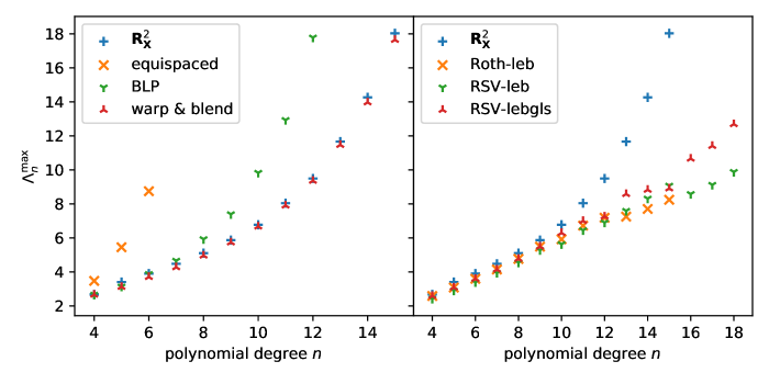
Figure 4: Lebesgue constants on the triangle, comparing $\boldsymbol{R}^{2}_{\boldsymbol{X}}$ against node families defined explicitly (left) and implicitly (right).

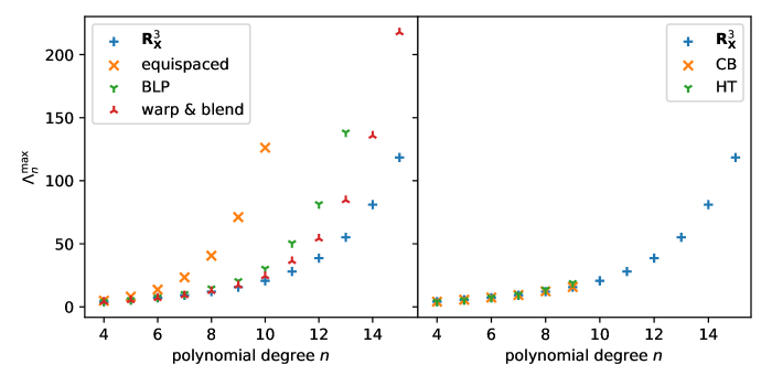
Figure 5: Lebesgue constants on the tetrahedron, comparing $\boldsymbol{R}^{3}_{\boldsymbol{X}}$ against node families defined explicitly (left) and implicitly (right).

Lebesgue constants for $\boldsymbol{R}^{d}_{\boldsymbol{X}}$ are compared against some other node families on the triangle in Fig. 4 and on the tetrahedron in Fig. 5. These include:

• equispaced: Equispaced nodes, defined by $b_{\text{eq},i}(\boldsymbol{\alpha})=\alpha_{i}/|\boldsymbol{\alpha}|$.

• BLP: The nodes of Blyth, Luo, & Pozrikidis [BP06],[LP06], which like the recursively defined nodes are based on the LGL nodes $\boldsymbol{X}_{\text{LGL}}$. If $\boldsymbol{\alpha}>0$, which indicates that the node will be in the interior of the simplex, they are defined by

  $$b_{\text{BLP},i}(\boldsymbol{\alpha})=\frac{1}{|\boldsymbol{\alpha}|}(1+|\boldsymbol{\alpha}|x_{|\boldsymbol{\alpha}|,\alpha_{i}}-{\textstyle\sum_{j}}\,x_{|\boldsymbol{\alpha}|,\alpha_{j}}).$$

  Points on the boundary are mapped from the same rule applied to the $(d-1)$-simplex.

• warp & blend: The nodes of [War06], which define the node location $\boldsymbol{b}_{\text{wb}}(\boldsymbol{\alpha})$ as the image of the equispaced node $\boldsymbol{b}_{\text{eq}}(\boldsymbol{\alpha})$ under a smooth bijection of the $d$-simplex. The bijection sends equispaced nodes to LGL nodes on the edges. The smooth map is nearly isoparametric, but a blending parameter is introduced that controls the distortion in the interior of the element, and optimal values of this blending parameter have been computed for $n$ up to $15$ in $d=2$ and $3$.

• Roth-leb: Nodes for the triangle computed by [Rot05] by numerical minimization of $\Lambda_{n}^{\max}$.

• RSV-leb: Nodes for the triangle computed by [RSV12] by numerical minimization of $\Lambda_{n}^{\max}$.

• RSV-lebgls: Nodes for the triangle computed by [RSV12] by numerical minimization of $\Lambda_{n}^{\max}$, subject to the constraints that the nodes remain symmetric and that the nodes on the edges be LGL nodes.

• CB: Nodes for the tetrahedron computed by [CB96] by numerical minimization of the related interpolation metric

  $$\Lambda_{n}^{2}(X)=\int_{\Delta^{d}}\sum_{\varphi\in\Phi_{X}}\varphi(\boldsymbol{x})^{2}\ dx.$$

• HT: Nodes for the tetrahedron computed by [HT00] as the equilibrium distribution of charged particles.

All of these node families except Roth-leb and RSV-leb are symmetric for all $n$, and all except equispaced, Roth-leb, and RSV-leb have edge traces that are LGL nodes. The equispaced, BLP, and warp & blend nodes can be explicitly defined in any dimension and have the recursive boundary property (III) from Section 3.1.

Both Figs. 4 and 5 split the comparison of the $\boldsymbol{R}^{d}_{\boldsymbol{X}}$ node family into comparisons against families that are explicitly defined and nodes that are implicitly defined as the solution of an optimization problem.

2D: In 2D, the $\boldsymbol{R}^{2}_{\boldsymbol{X}}$ node family has Lebesgue constants that are not much worse than those for node families implicitly defined to minimize the Lebesgue constant for $n\leq 9$ (Fig. 4, left). For $n\geq 10$, the Lebesgue constant grows much faster for $\boldsymbol{R}^{2}_{\boldsymbol{X}}$ than for the best implicitly defined nodes.

Not coincidentally, at $n=10$ the layout of implicitly defined nodes that minimize the Lebesgue constant changes significantly. Until then, the RSV-lebgls nodes look “lattice-like,” as though they have been smoothly, symmetrically, and monotonically mapped from the equispaced nodes, the same as the explicit node families. At $n=10$, however, this pattern changes (Fig. 6). This suggests that no node family that retains the lattice-like structure, including $\boldsymbol{R}^{d}_{\boldsymbol{X}}$, can attain a slow growth of $\Lambda_{n}^{\max}$ like the implicitly defined families.

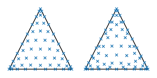
Figure 6: The LEBGLS nodes of [RSV12], showing the abrupt change in layout between $n=9$ (left) and $n=10$ (right).

In comparison to the other explicitly defined nodes (Fig. 4, right), the $\boldsymbol{R}^{2}_{\boldsymbol{X}}$ family is nearly as good as the warp & blend family, which has the best Lebesgue constants: $\Lambda_{n}^{\max}$ is never more than $10\%$ different between them for $n\leq 15$. In fact, despite the differences in their definitions—warp & blend by continuous bijections, $\boldsymbol{R}^{2}_{\boldsymbol{X}}$ by recursion—the node families are remarkably similar for $n\leq 15$: $\|\boldsymbol{b}_{\boldsymbol{X}}(\alpha)-\boldsymbol{b}_{\text{wb}}(\alpha)\|\leq 0.01$ for every node in these node sets.

3D: In 3D there are no published examples of $\Lambda_{n}^{\max}$-optimal node sets that have been numerically computed in the same way as in 2D. $\Lambda_{n}^{\max}(X)$ is a nonconvex function of the node coordinates in $X$, and the number of coordinates grows cubically with $n$, so this is a challenging optimization problem. Instead, the implicitly defined node families CB and HT optimize simpler objectives: the $\Lambda_{n}^{2}$ interpolation metric and the electrostatic potential, respectively, and these have only been computed to $n\leq 9$. There is little difference in $\Lambda_{n}^{\max}$ between $\boldsymbol{R}^{3}_{\boldsymbol{X}}$ and these two families (Fig. 5, left), though it is slightly smaller than both for $n\geq 6$.

In comparison to the explicitly defined node families BLP and warp & blend (Fig. 5, right), there is little difference for $n\leq 6$ (all are within $7\%$ of each other), but $\boldsymbol{R}^{3}_{\boldsymbol{X}}$ is increasingly superior for $n\geq 7$. For $n=15$, the largest for which the warp & blend nodes’ blending parameter has been optimized, the Lebesgue constant of $\boldsymbol{R}^{3}_{\boldsymbol{X}}$ is $40\%$ smaller.

3.3 Asymptotic interpolation properties

A node family is good for approximation by interpolation if the interpolants are known to converge for a large class of functions. In particular, if $f$ is analytic in the neighborhood of $\Delta^{d}$, then there is a sequence of polynomials $p_{n}\rightrightarrows f$ (converging uniformly on $\Delta^{d}$), so it is possible that given the right node family $\boldsymbol{X}=\{X_{n}\}$ that $I_{X_{n}}f\rightrightarrows f$ for all analytic $f$ as well.

The weakest known sufficient condition that guarantees this for $d>1$ is sub-exponential growth of the Lebesgue constant: if $\Lambda_{n}^{\max}(X_{n})^{1/n}\to 1$, then $I_{X_{n}}f\rightrightarrows f$ for $f$ analytic in a neighborhood of $\Delta^{d}$ [Blo+92]. The values of $\Lambda_{n}^{\max}(R^{d}_{\boldsymbol{X},n})$ that appeared in Figs. 4 & 5 are tabulated in Table LABEL:tab:lebtable. In all tabulated values, $(\Lambda_{n}^{\max})^{1/n}$ continues to increase instead of converging to 1, so they show no evidence of sub-exponential growth.

Table 1: Lebesgue constants computed for $\boldsymbol{R}^{d}_{\boldsymbol{X}}$

$n$	$\Lambda_{n}^{\max}(R^{2}_{\boldsymbol{X},n})$	$\Lambda_{n}^{\max}(R^{2}_{\boldsymbol{X},n})^{1/n}$	$\Lambda_{n}^{\max}(R^{3}_{\boldsymbol{X},n})$	$\Lambda_{n}^{\max}(R^{3}_{\boldsymbol{X},n})^{1/n}$
4	2.67857	1.27931	4.09308	1.42237
5	3.40745	1.27787	5.54727	1.40869
6	3.90448	1.25486	7.16891	1.38859
7	4.47897	1.23887	9.20205	1.37309
8	5.10406	1.226	12.0671	1.36521
9	5.87268	1.21738	15.5927	1.3569
10	6.77248	1.21081	20.6234	1.35343
11	8.04267	1.20867	28.034	1.35397
12	9.49527	1.20631	38.6495	1.35601
13	11.6647	1.208	55.1425	1.36132
14	14.2678	1.20908	81.0374	1.36878
15	18.0306	1.21265	118.42	1.37476

In fact, [Blo+92] considered it an open question whether explicitly computed node families with uniformly convergent interpolants exist for any nontrivial set in $d>1$. In the intervening time, analogues of the Chebyshev polynomials have been found for domains related to root systems [RM10], but these domains are not simplices. [Blo+12] considered the question still open for simplices twenty years later, and it appears to still be open now.

3.4 Finite element matrix conditioning

Matrices that show up repeatedly in applications of the finite element method include the mass matrix $M_{ij}=\int_{\Delta^{d}}\varphi_{i}\varphi_{j}\ dx$ and the stiffness matrix $K_{ij}=\int_{\Delta^{d}}\nabla\varphi_{n,i}\cdot\nabla\varphi_{n,j}\ dx$. Let $G_{ijk}=\partial_{j}\varphi_{k}(\boldsymbol{x}_{i})$ (considered as a matrix in $\mathbb{R}^{d|\Phi|\times|\Phi|}$), and $L_{ij}=\nabla\cdot\nabla\varphi_{j}(\boldsymbol{x}_{i})$. These are the nodal gradient and Laplacian matrices, that appear in strong-form nodal discontinuous Galerkin methods. The condition numbers of these matrices (using the definition $\kappa_{2}(A)=\|A\|_{2}\|A^{\dagger}\|_{2}$) for $\boldsymbol{R}^{d}_{\boldsymbol{X}}$ are compared against the condition numbers for the equispaced, BLP, warp & blend, and RSV-lebgls nodes in Fig. 7. The condition number of $M$ is affine invariant and in a quasiuniform mesh bounds the condition number of a fully assembled mass matrix [Wat87], while the condition numbers of $K$, $G$, and $L$ depend on the choice of reference simplex: in this work, they are computed with respect to the biunit simplex $\Delta^{d}_{\text{bi}}=\{\boldsymbol{x}\in\mathbb{R}^{d}:\boldsymbol{x}\geq-1,\ \sum_{i}x_{i}\leq 2-d\}$. The rankings of the node families by these metrics are essentially the same as by the Lebesgue constant in Section 3.2.

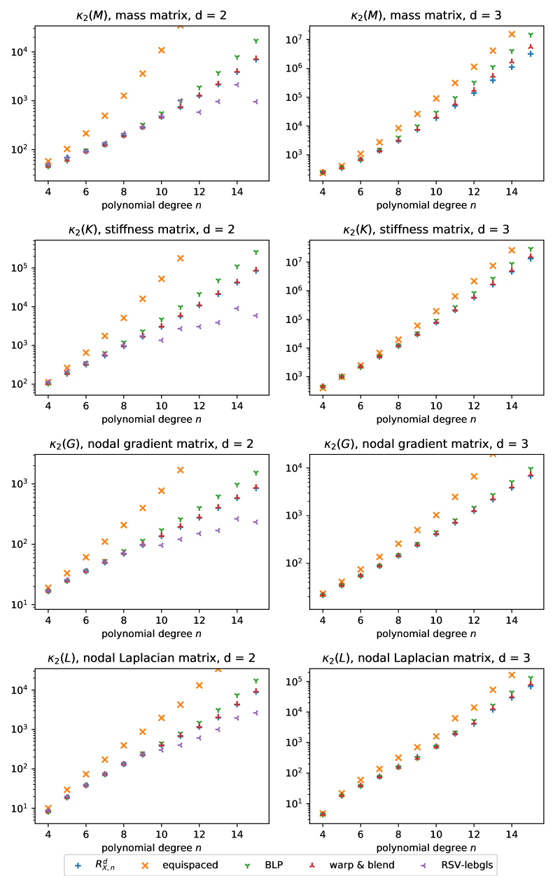
Figure 7: Condition numbers of finite element matrices.

Table 2: Finite element matrix condition numbers $\boldsymbol{R}^{2}_{\boldsymbol{X}}$

$n$	$\kappa_{2}(M)$	$\kappa_{2}(M)^{1/n}$	$\kappa_{2}(K)$	$\kappa_{2}(K)^{1/n}$	$\kappa_{2}(G)$	$\kappa_{2}(G)^{1/n}$	$\kappa_{2}(L)$	$\kappa_{2}(L)^{1/n}$
4	4.7e+01	2.618	1.0e+02	3.196	1.7e+01	2.022	8.2e+00	1.691
8	2.0e+02	1.933	9.5e+02	2.358	7.0e+01	1.700	1.3e+02	1.840
16	1.3e+04	1.808	1.7e+05	2.124	1.2e+03	1.561	1.9e+04	1.848
24	2.8e+06	1.856	6.3e+07	2.113	2.8e+04	1.532	7.4e+06	1.933
32	8.0e+08	1.898	2.5e+10	2.114	6.2e+05	1.517	3.2e+09	1.982

Table 3: Finite element matrix condition numbers $\boldsymbol{R}^{3}_{\boldsymbol{X}}$

$n$	$\kappa_{2}(M)$	$\kappa_{2}(M)^{1/n}$	$\kappa_{2}(K)$	$\kappa_{2}(K)^{1/n}$	$\kappa_{2}(G)$	$\kappa_{2}(G)^{1/n}$	$\kappa_{2}(L)$	$\kappa_{2}(L)^{1/n}$
4	2.5e+02	3.977	4.5e+02	4.615	2.2e+01	2.158	4.4e+00	1.449
8	3.1e+03	2.734	1.2e+04	3.231	1.4e+02	1.862	1.6e+02	1.889
12	1.4e+05	2.682	5.8e+05	3.022	1.3e+03	1.812	4.1e+03	2.001
16	9.3e+06	2.726	3.8e+07	2.979	1.2e+04	1.798	1.8e+05	2.132

In Tables LABEL:tab:condtable and LABEL:tab:condtable3 the growth rates of these condition numbers can be assessed. The values of $\kappa_{2}(M)^{1/n}$, $\kappa_{2}(K)^{1/n}$ and $\kappa_{2}(L)^{1/n}$ are not monotonically decreasing in both dimensions for values of $n$ that have been calculated, which suggests super-exponential growth. $\kappa_{2}(G)^{1/n}$ appears to be monotonically decreasing towards some limit $\gamma_{d}>1$ for $d=2$, and $d=3$, which suggests exponential growth, but there is no proof of this fact.

3.5 Finite element matrix efficiency

To evaluate the basis functions of $R^{d}_{\boldsymbol{X},n}$ at a set of nodes $Q$, one can compute the Vandermonde matrices $V_{R^{d}_{\boldsymbol{X},n}}$ and $V_{Q}$ with respect to a stable basis for $\mathcal{R}_{n}(\Delta^{d})$, such as the Proriol-Koornwinder-Dubiner basis [Pro57],[Koo75],[Dub91], and assemble $V_{Q}V_{R^{d}_{\boldsymbol{X},n}}^{-1}$. This approach goes back at least to [WPH00], and was improved with a singularity-free evaluation of the basis by [Kir10a]. Assuming $|Q|\in\Theta(n^{d})$, the cost of constructing this matrix is $\Theta(n^{3d})$. There is no structure in $R^{d}_{\boldsymbol{X},n}$ that would allow for fast application to a vector of nodal coefficients, so the cost of a matrix vector product is $\Theta(n^{2d})$. The same costs hold for each directional derivative of the basis functions.

There appears to be no Lagrange polynomial basis for $\mathcal{R}_{n}(\Delta^{d})$ that improves on this for $d>1$, so all of the node families discussed above are equal with respect to this metric. It must be noted, however, that outside of Lagrange bases are bases that have fast algorithms, either through hierarchical construction, like Bernstein-Bézier polynomials, or through generalized tensor-product constructions related to the Duffy transformation, like the basis of [SK95]. The Bernstein-Bézier basis has been the subject of more recent work, and has fast algorithms that allow for optimal construction in $\Theta(n^{2d})$ and application in $\Theta(n^{d})$ for these matrices, for constant coefficients matrices without quadrature [Kir10], for evaluation at the Stroud quadrature points [AAD11], and for the inverse of the mass matrix [Kir16]. A drawback of the Bernstein-Bézier basis is mass-matrix condition numbers $\kappa_{2}(n,d)=\binom{2n+d}{n}$ that are worse even than equispaced nodes, though recent work by [AK20] shows that a condition number that uses a matrix norm based on the $L_{2}$ norm of the reconstructed polynomials grows like $\sqrt{\kappa_{2}(n,d)}$.

3.6 Ease of computation and implementation

Implicitly defined node families, including Roth-leb, RSV-leb, RSV-lebgls, CB, and HT from Section 3.2 and others not discussed, require the solution of an optimization problem over the choice of node coordinates, a problem size that, even with symmetries enforced, is $\Theta(n^{d})$ in $n$. Objective functions like $\Lambda_{n}^{\max}(X)$ are quite nonconvex, so care must be taken to avoid local minima. It is fair to characterize these node sets as relatively expensive to compute from scratch.

The ease of implementing node sets from a node family is distinct from the computational complexity of computing the node sets from scratch. Most of the implicitly defined node sets discussed in this work have published node sets for moderate values of $n$ for $d=2$ [CB95][Hes98][RSV12], and a few for $d=3$ [CB96][HT00].

Of the explicitly defined node families discussed in this work, the equispaced and BLP nodes are the cheapest to compute: the former requires $\Theta(d)$ operations and $\Theta(1)$ workspace, the latter requires $\Theta(d^{2})$ operations and $\Theta(1)$ workspace per node. The warp & blend nodes additionally require $d+1$ evaluations of 1D Jacobi polynomials up to degree $n$ at each node (one per facet of the simplex) and one $\Theta(n^{3})$ inversion of a 1D Vandermonde matrix of size $n+1$ per node set.

The computational complexity of computing one node $\boldsymbol{b}_{\boldsymbol{X}}(\boldsymbol{\alpha})$ in isolation by the rule (1) satisfies the recursion $T(d)=(d+1)T(d-1)+\Theta(d^{2})$, which implies $T(d)\in\Theta((d+1)!)$. The workspace satisfies the recursion $S(d)=S(d-1)+\Theta(d)$, so $S(d)\in\Theta(d^{2})$. Neither of these are a concern for $d=2$ or $3$.

If the nodes must be computed for higher dimensions, the cost of computing a full node set can be reduced by caching the lower-dimensional nodes. Then the cost of computing the node sets $\{R^{d}_{\boldsymbol{X},i}\}_{i=0}^{n}$ with caching satisfies the recursion $T(d,n)=T(d-1,n)+\Theta(\binom{n+d+1}{d+1}d^{2})$, which implies $T(d,n)\in O(\binom{n+d+2}{d+1}d^{2})$, leading to an amortized cost per node that is $O((n+d)d^{2}/n)$. The workspace with caching satisfies the recursion $S(d,n)=S(d-1,n)+\Theta(\binom{n+d+1}{d+1}d)$, so $S(d,n)\in O(\binom{n+d+2}{d+1}d)$, which is an amortized space per node that is $O((n+d)d/n)$.

In terms of implementation, once the 1D node family $\boldsymbol{X}$ is available, the code to compute $\boldsymbol{b}_{\boldsymbol{X}}(\boldsymbol{\alpha})$ is very short. Here is an example implementation in python:

import numpy as np

def recursive(alpha, family):

    ’’’The barycentric d-simplex coordinates for a multi-index

    alpha with length d+1 and sum n, based on a 1D node family.’’’

    d = len(alpha) - 1

    n = sum(alpha)

    xn = family[n]

    b = np.zeros((d+1,))

    if d == 1:

        b[:] = xn[[alpha[0], alpha[1]]]

        return b

    weight = 0.

    for i in range(d+1):

        alpha_noti = alpha[:i] + alpha[i+1:]

        w = xn[n - alpha[i]]

        br = recursive(alpha_noti, family)

        b[:i] += w * br[:i]

        b[i+1:] += w * br[i:]

        weight += w

    b /= weight

    return b

A reference python implementation, which includes all numerical methods used to evaluate and compare against other node families in this work, is available as the recursivenodes package [Isa20]. The website for the package [Isa20a] hosts a version of this manuscript showing how it was used to generate all figures and tables.

4 Using 1D families other than LGL nodes

The analysis and comparison in Section 3 was conducted under the assumption that the 1D node family $\boldsymbol{X}$ was $\boldsymbol{X}_{\text{LGL}}$, the Lobatto-Gauss-Legendre nodes on the interval $[0,1]$. The recursive rule (1) allows for an arbitrary 1D node family. While $\boldsymbol{X}_{\text{LGL}}$ appears to be the best choice according to the metrics in Section 3, for completeness a few alternate choices of $\boldsymbol{X}$ are presented here.

$\boldsymbol{X}_{\text{eq}}$ (equispaced): It is not surprising, given the discussion in Section 2 where equispaced nodes provided the intuition behind the recursive rule, that using $\boldsymbol{X}=\boldsymbol{X}_{\text{eq}}$ reproduces the equispaced nodes, $\boldsymbol{b}_{\boldsymbol{X}_{\text{eq}}}(\boldsymbol{\alpha})=\boldsymbol{b}_{\text{eq}}(\boldsymbol{\alpha})$.

$\boldsymbol{X}_{\text{LGC}}$ (Lobatto-Gauss-Chebyshev): The 1D Lobatto-Gauss-Chebyshev (LGC) node family has good interpolation properties in 1D while being a nested family, with $X_{n,\text{LGC}}\subset X_{2n,\text{LGC}}.$ The recursive nodes $\boldsymbol{R}^{d}_{\boldsymbol{X}_{\text{LGC}}}$ inherit the nested property, as demonstrated in Fig. 8, left.

$\boldsymbol{X}_{\text{GL}}$ (Gauss-Legendre): The 1D Gauss-Legendre (GC) node family does not include the endpoints $0$ and $1$, but can still be used to construct nodes. Property (III) in Section 3.1 does not hold, and in fact all nodes will be in the interior of the $d$-simplex as demonstrated in Fig. 8, right.

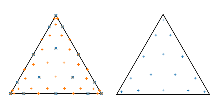
Figure 8: (left) The node sets $R^{2}_{\boldsymbol{X}_{\text{LGC}},4}$ and $R^{2}_{\boldsymbol{X}_{\text{LGC}},8}$, demonstrating nested node sets, a property inherited from the 1D LGC node family. (right) The node set $R^{2}_{\boldsymbol{X}_{\text{GL}},4}$, demonstrating node sets contained in the interior.

The metrics from Section 3 are used to compare $\boldsymbol{R}^{d}_{\boldsymbol{X}}$ for $\boldsymbol{X}_{\text{LGL}}$, $\boldsymbol{X}_{\text{LGC}}$, and $\boldsymbol{X}_{\text{GL}}$ in Fig. 9. The results for $d=2$ and $d=3$ resemble the results of the 1D node families, with GL nodes having worse interpolation properties but better conditioned mass matrices than either set of Lobatto nodes, and with LGC nodes having interpolation properties and matrix condition numbers that similar but slightly worse to LGL nodes. The most interesting trend to be observed in Fig. 9 is that, while the growth rate of the Lebesgue constant for the GL nodes is worse than the Lobatto nodes in 2D, it is much closer in 3D.

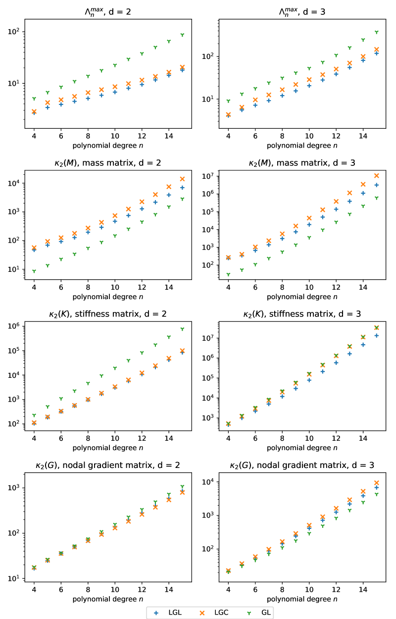
Figure 9: Comparing $\boldsymbol{R}^{d}_{\boldsymbol{X}_{\text{LGL}}}$, $\boldsymbol{R}^{d}_{\boldsymbol{X}_{\text{LGC}}}$, and $\boldsymbol{R}^{d}_{\boldsymbol{X}_{\text{GL}}}$ according to metrics from Section 3.

5 Interpolation tests

To show that the bounds implied by the Lebesgue constants in 3.2 are in line with interpolation errors in practice, this section compares those errors for the recursively constructed nodes against other node families for two benchmark functions that have appeared previously.

The first function is

$$f_{A}(\boldsymbol{x})=\prod_{i}(x_{i}+1)\cosh\left(\sum_{i}x_{i}-1\right),$$ (6)

which has appeared in [Hei05][War06][CW15] as an example of a smooth, non-polynomial function to which even the equispaced polynomial interpolants converge. In Table LABEL:tab:interperr_smooth, the absolute interpolation errors $\|I_{X}(f_{A})-f_{A}\|_{\infty}$ on the biunit simplex is tested for node families that appeared in Section 3.

The next is the “Witch of Agnesi” function,

$$f_{B}(\boldsymbol{x})=\frac{1}{1+\alpha|\boldsymbol{x}|^{2}},$$ (7)

which for $\alpha=25$ is the classic Runge function, for which the equispaced interpolants diverge in some domains. Table LABEL:tab:interperr_runge reports $\|I_{X}(f_{B})-f_{B}\|_{\infty}$ on an equilateral simplex centered at the origin with edge length 2. For $d=2$, the standard $\alpha=25$ is used, but for $d=3$, $\alpha=60$ is used instead to make errors of the equispaced interpolants roughly the same as for $d=2$.

Table 4: Interpolation errors $\|I_{X}(f_{A})-f_{A}\|_{\infty}$

$d$	$n$	equispaced	BLP	warp & blend	RSV-lebgls	${\boldsymbol{R}}^{d}_{\boldsymbol{X}}$
2	6	3.6e-04	2.6e-04	2.4e-04	2.4e-04	2.2e-04
2	9	2.7e-07	2.4e-07	1.7e-07	1.6e-07	1.6e-07
2	12	7.9e-11	7.3e-11	3.6e-11	1.5e-11	3.6e-11
2	15	6.2e-14	1.5e-14	8.4e-15	5.1e-15	8.7e-15
2	18	4.1e-13	1.3e-14	1.6e-14	6.0e-15	4.9e-15
3	6	1.1e-03	8.4e-04	8.1e-04	-	7.8e-04
3	9	9.5e-07	1.6e-06	1.3e-06	-	1.1e-06
3	12	4.0e-10	1.1e-09	7.4e-10	-	4.6e-10
3	15	1.2e-13	3.6e-13	1.8e-13	-	9.0e-14
3	18	6.3e-13	9.9e-14	-	-	4.6e-14

Table 5: Interpolation errors $\|I_{X}(f_{B})-f_{B}\|_{\infty}$

$d$	$n$	equispaced	BLP	warp & blend	RSV-lebgls	${\boldsymbol{R}}^{d}_{\boldsymbol{X}}$
2	6	4.5e-01	3.0e-01	3.1e-01	3.0e-01	3.1e-01
2	9	6.6e-01	2.4e-01	1.7e-01	1.7e-01	1.7e-01
2	12	1.1e+00	2.6e-01	9.8e-02	7.9e-02	9.9e-02
2	15	1.9e+00	3.0e-01	6.2e-02	4.4e-02	6.8e-02
2	18	3.1e+00	3.5e-01	2.7e-01	2.3e-02	4.9e-02
3	6	6.5e-01	6.9e-01	7.1e-01	-	7.4e-01
3	9	4.1e-01	4.9e-01	5.1e-01	-	5.6e-01
3	12	1.0e+00	1.6e+00	7.7e-01	-	2.3e-01
3	15	1.9e+00	2.4e+00	9.0e-01	-	1.4e-01
3	18	4.5e+00	4.3e+00	-	-	1.3e-01

The relative sizes of the interpolation errors in Tables LABEL:tab:interperr_smooth and LABEL:tab:interperr_runge more or less correspond to the relative sizes of the Lebesgue constants. For the more difficult function $f_{B}$ the recursive nodes $\boldsymbol{R}^{3}_{\boldsymbol{X}}$ continue to converge at $n=18$ when the other node sets have already begun to diverge.

6 Conclusion

How and by whom should the nodes $\boldsymbol{R}^{d}_{\boldsymbol{X}}$ defined by the recursive rule (1) be used? The comparisons in this paper have made the case that is the best explicit construction rule thus far, because of its simplicity, its symmetry, and its performance in the metrics that matter to finite element construction (but not for producing asymptotically convergent interpolants). It does not outperform the Warburton’s warp & blend node family in 2D, so software already using those would not benefit from switching, but its performance is superior to all other explicit node families in 3D, particularly for $n\geq 7$. Likewise, where implicitly defined node families—such as Rapetti, Sommariva, and Vianello’s LEBGLS nodes—have been computed and published, they are superior to the $\boldsymbol{R}^{d}_{\boldsymbol{X}}$ node family, especially in 2D for $n\geq 10$. But at the time of this writing the tetrahedron has not received nearly as much attention as the triangle, and so this new node family is the best available in 3D.

In Section 3.1 it was argued that the edge trace property was useful in aligning nodes with tensor-product cells in hybrid meshes. In 3D, a further necessary condition is for the traces on triangular facets to align with neighboring nodes pyramid cells. There is no perfect analogue for the overdetermined projections (4) in the pyramid, so the development of a matching node construction for the pyramid is left for future work, where it would have to be compared against existing node sets such as those developed by [CW15].

7 Acknowledgements

The methods in this work were discovered in the course of research funded by grant #DE-SC0016140 from the U.S. Department of Energy’s Office of Advanced Scientific Research. The author also thanks the anonymous referees who suggested additional references and improvements to this work.

References

- [AAD11] Mark Ainsworth, Gaelle Andriamaro and Oleg Davydov “Bernstein–Bézier Finite Elements of Arbitrary Order and Optimal Assembly Procedures” In SIAM Journal on Scientific Computing 33.6 Society for Industrial & Applied Mathematics (SIAM), 2011, pp. 3087–3109 DOI: 10.1137/11082539x
- [AK20] Larry Allen and Robert C. Kirby “Structured Inversion of the Bernstein Mass Matrix” In SIAM Journal on Matrix Analysis and Applications 41.2 Society for Industrial & Applied Mathematics (SIAM), 2020, pp. 413–431 DOI: 10.1137/19m1284166
- [Blo+12] T. Bloom, L.. Bos, J.-P. Calvi and N. Levenberg “Polynomial interpolation and approximation in ” In Annales Polonici Mathematici 106 Institute of Mathematics, Polish Academy of Sciences, 2012, pp. 53–81 DOI: 10.4064/ap106-0-5
- [Blo+92] T. Bloom, L. Bos, C. Christensen and N. Levenberg “Polynomial Interpolation of Holomorphic Functions in and ” In Rocky Mountain Journal of Mathematics 22.2 Rocky Mountain Mathematics Consortium, 1992, pp. 441–470 DOI: 10.1216/rmjm/1181072740
- [BP06] M.. Blyth and C. Pozrikidis “A Lobatto interpolation grid over the triangle” In IMA Journal of Applied Mathematics 71.1 Oxford University Press (OUP), 2006, pp. 153–169 DOI: 10.1093/imamat/hxh077
- [CB95] Qi Chen and Ivo Babuška “Approximate optimal points for polynomial interpolation of real functions in an interval and in a triangle” In Computer Methods in Applied Mechanics and Engineering 128.3-4 Elsevier BV, 1995, pp. 405–417 DOI: 10.1016/0045-7825(95)00889-6
- [CB96] Qi Chen and Ivo Babuška “The optimal symmetrical points for polynomial interpolation of real functions in the tetrahedron” In Computer Methods in Applied Mechanics and Engineering 137.1 Elsevier BV, 1996, pp. 89–94 DOI: 10.1016/0045-7825(96)01051-1
- [CW15] Jesse Chan and T. Warburton “A Comparison of High Order Interpolation Nodes for the Pyramid” In SIAM Journal on Scientific Computing 37.5 Society for Industrial & Applied Mathematics (SIAM), 2015, pp. A2151–A2170 DOI: 10.1137/141000105
- [Dub91] Moshe Dubiner “Spectral methods on triangles and other domains” In Journal of Scientific Computing 6.4 Springer ScienceBusiness Media LLC, 1991, pp. 345–390 DOI: 10.1007/bf01060030
- [Hei05] Wilhelm Heinrichs “Improved Lebesgue constants on the triangle” In Journal of Computational Physics 207.2 Elsevier BV, 2005, pp. 625–638 DOI: 10.1016/j.jcp.2005.02.002
- [Hes98] J.. Hesthaven “From Electrostatics to Almost Optimal Nodal Sets for Polynomial Interpolation in a Simplex” In SIAM Journal on Numerical Analysis 35.2 Society for Industrial & Applied Mathematics (SIAM), 1998, pp. 655–676 DOI: 10.1137/s003614299630587x
- [HT00] J.. Hesthaven and C.. Teng “Stable Spectral Methods on Tetrahedral Elements” In SIAM Journal on Scientific Computing 21.6 Society for Industrial & Applied Mathematics (SIAM), 2000, pp. 2352–2380 DOI: 10.1137/s1064827598343723
- [Isa20] Tobin Isaac “recursivenodes: Recursive, parameter-free, explicitly defined interpolation nodes for simplices” Zenodo, 2020 DOI: 10.5281/zenodo.3675431
- [Isa20a] Tobin Isaac “recursivenodes: Recursive, parameter-free, explicitly defined interpolation nodes for simplices”, 2020 URL: https://tisaac.gitlab.io/recursivenodes
- [Kir10] Robert C. Kirby “Fast simplicial finite element algorithms using Bernstein polynomials” In Numerische Mathematik 117.4 Springer ScienceBusiness Media LLC, 2010, pp. 631–652 DOI: 10.1007/s00211-010-0327-2
- [Kir10a] Robert C. Kirby “Singularity-free evaluation of collapsed-coordinate orthogonal polynomials” In ACM Transactions on Mathematical Software 37.1 Association for Computing Machinery (ACM), 2010, pp. 1–16 DOI: 10.1145/1644001.1644006
- [Kir16] Robert C. Kirby “Fast inversion of the simplicial Bernstein mass matrix” In Numerische Mathematik 135.1 Springer ScienceBusiness Media LLC, 2016, pp. 73–95 DOI: 10.1007/s00211-016-0795-0
- [Koo75] Tom Koornwinder “Two-Variable Analogues of the Classical Orthogonal Polynomials” In Theory and Application of Special Functions Elsevier, 1975, pp. 435–495 DOI: 10.1016/b978-0-12-064850-4.50015-x
- [LP06] H. Luo and C. Pozrikidis “A Lobatto interpolation grid in the tetrahedron” In IMA Journal of Applied Mathematics 71.2 Oxford University Press (OUP), 2006, pp. 298–313 DOI: 10.1093/imamat/hxh111
- [Pro57] Joseph Proriol “Sur une famille de polynomes á deux variables orthogonaux dans un triangle” In Comptes Rendus Hebdomadaires Des Seances De L’Academie Des Sciences 245.26 Gauthier-Villars/Editions Elsevier 23 Rue Linois, 75015 Paris, France, 1957, pp. 2459–2461
- [RM10] Brett N. Ryland and Hans Z. Munthe-Kaas “On Multivariate Chebyshev Polynomials and Spectral Approximations on Triangles” In Spectral and High Order Methods for Partial Differential Equations Springer Berlin Heidelberg, 2010, pp. 19–41 DOI: 10.1007/978-3-642-15337-2_2
- [Rot05] Michael James Roth “Nodal configurations and Voronoi tessellations for triangular spectral elements”, 2005 URL: http://hdl.handle.net/1828/44
- [RSV12] Francesca Rapetti, Alvise Sommariva and Marco Vianello “On the generation of symmetric Lebesgue-like points in the triangle” In Journal of Computational and Applied Mathematics 236.18 Elsevier BV, 2012, pp. 4925–4932 DOI: 10.1016/j.cam.2011.11.023
- [SK95] Spencer J. Sherwin and George Em Karniadakis “A new triangular and tetrahedral basis for high-order (hp) finite element methods” In International Journal for Numerical Methods in Engineering 38.22 Wiley, 1995, pp. 3775–3802 DOI: 10.1002/nme.1620382204
- [War06] T. Warburton “An explicit construction of interpolation nodes on the simplex” In Journal of Engineering Mathematics 56.3 Springer ScienceBusiness Media LLC, 2006, pp. 247–262 DOI: 10.1007/s10665-006-9086-6
- [Wat87] A.. Wathen “Realistic Eigenvalue Bounds for the Galerkin Mass Matrix” In IMA Journal of Numerical Analysis 7.4 Oxford University Press (OUP), 1987, pp. 449–457 DOI: 10.1093/imanum/7.4.449
- [WPH00] T. Warburton, L.F. Pavarino and J.S. Hesthaven “A Pseudo-spectral Scheme for the Incompressible Navier–Stokes Equations Using Unstructured Nodal Elements” In Journal of Computational Physics 164.1 Elsevier BV, 2000, pp. 1–21 DOI: 10.1006/jcph.2000.6587