Excitation Transport in Molecular Aggregates with thermal motion

Abstract

Molecular aggregates can under certain conditions transport electronic excitation energy over large distances due to dipole-dipole interactions. Here, we explore to what extent thermal motion of entire monomers can guide or enhance this excitation transport. The motion induces changes of aggregate geometry and hence modifies exciton states. Under certain conditions, excitation energy can thus be transported by the aggregate adiabatically, following a certain exciton eigenstate. While such transport is always slower than direct migration through dipole-dipole interactions, we show that transport through motion can yield higher transport efficiencies in the presence of on-site energy disorder than the static counterpart. For this we consider two simple models of molecular motion: (i) longitudinal vibrations of the monomers along the aggregation direction within their inter-molecular binding potential and (ii) torsional motion of planar monomers in a plane orthogonal to the aggregation direction. The parameters and potential shapes used are relevant to dye-molecule aggregates. We employ a quantum-classical method, in which molecules move through simplified classical molecular dynamics, while the excitation transport is treated quantum mechanically using Schrödinger’s equation. For both models we find parameter regimes in which the motion enhances excitation transport, however these are more realistic for the torsional scenario, due to the limited motional range in a typical Morse type inter-molecular potential. We finally show that the transport enhancement can be linked to adiabatic quantum dynamics. This transport enhancement through adiabatic motion appears a useful resource to combat exciton trapping by disorder.

I Introduction

Molecular aggregates in which a large number of organic molecules assemble into a fairly regular structure can exhibit significant excitation energy transport along the structure Brixner et al. (2017); Haedler et al. (2016), which plays a key role in photosynthetic light harvesting processes van Amerongen et al. (2000); van Grondelle and Novoderezhkin (2006) and has the potential for technological exploitation, e.g. in dye-sensitized solar cells Zhang and Cole (2017); Ghosh and Feng (1978) or thin-film optical and optoelectronic devices Malyshev et al. (2000). In all of these, molecular aggregates facilitate the absorption of light and subsequent transfer of the absorbed energy to a reaction centre Saikin et al. (2013); Macedo et al. (2019) in the form of an electron-hole pair known as exciton. This transfer of excitation relies on the long range dipole-dipole interactions between the monomers in the aggregate.

Such dipole-dipole interactions are also a characteristic feature of Rydberg aggregates Wüster and Rost (2018), which hence have been proposed as quantum simulators for molecular aggregates Schönleber et al. (2015); Hague and MacCormick (2012). In Rydberg aggregates, a chain of highly excited Rydberg atoms transports a single energy quantum on spatial- and temporal scales quite different from the molecular context. While the excitation transfer process in molecular aggregates is typically strongly affected by decoherence Kasha (1963); Chen and Silbey (2011); Roden et al. (2009); Haken and Reineker (1972), it barely is in ultra-cold atoms, as has been experimentally demonstrated Barredo et al. (2015); Labuhn et al. (2016); Marcuzzi et al. (2017).

An idea that naturally arises in Rydberg aggregates, is adiabatic excitation transport through atomic motion Wüster et al. (2010); Wüster and Rost (2018); Möbius et al. (2011). In adiabatic excitation transport, slow motion of the atoms combined with excitation transport via dipole-dipole interactions can result in efficient and guided transport of the excitation from one end of an atomic chain to the other, see schematic in Fig. 1 (a). Based on the analogy between Rydberg- and Molecular aggregates, the question then arises whether adiabatic excitation transport can play a functional role in molecular aggregates, e.g. for light harvesting.

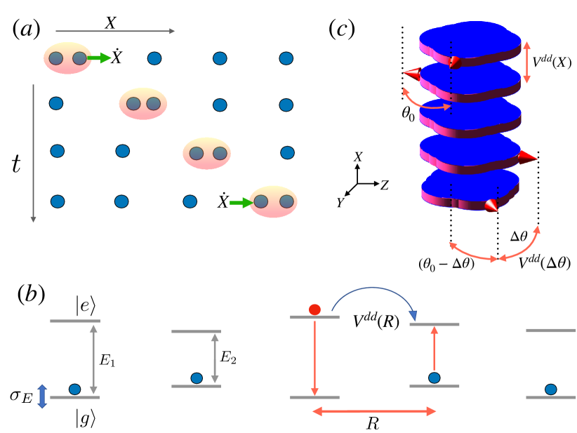
Figure 1: (a) Interplay of molecular motion and excitation transfer in adiabatic excitation transport. Blue $\bullet$ are molecules or atoms, $X$ indicates their position and $\dot{X}$ (green arrow) their velocity. The orange shade represents a selected de-localized exciton state. This state is always located on the two closest molecules, such that if the state is adiabatically followed, the indicated motion entails excitation transport. (b) Energy level schematic, with molecular electronic ground state $|\,{g}\,\rangle$ and excited state $|\,{e}\,\rangle$ and dipole-dipole interactions $V^{dd}(R)$. We also sketch on-site disorder $\sigma_{E}$ of transition energies. (c) More detailed sketch of a 1D chain of planar molecules with torsional motion along $\theta$ and longitudinal motion along $X$. (blue disk) molecules, (red large arrow) direction of the transition dipole moment axis between $|\,{g}\,\rangle$ and $|\,{e}\,\rangle$. $\theta_{0}$ is the relative nearest neighbour angle in equilibrium and $\Delta\theta$ possible angular disorder around this value.

Here we report initial explorations of this idea, ignoring for now the effect of the intra-molecular vibrations but including some effects of the protein environment as a static disorder in energy. Our model is then a closed quantum system for the excitation transport, and our main observables are derived from the dynamics of excitation population on different molecules, classically averaged over the disordered ensemble. The motivation for this framework is as follows: quantum adiabatic following in excitation transport was first reported in the atomic case where internal vibrations are absent Wüster et al. (2010). If we cannot find similar features in a molecular setting excluding internal vibrations, they are unlikely to be present in a case where vibrations are included, since these are known to significantly modify excitation transport Chen and Silbey (2011); Roden et al. (2009, 2012). We however shall find that adiabatic excitation transport persists and thus intend to explore in the future to what extent adiabatic excitation transport can survive the coupling to internal molecular vibrations. Meanwhile, our results should already be applicable to some extent to those molecular aggregates where the coupling of excitons with internal vibrations is weak, such as those reported in Eisfeld and Briggs (2002); Haedler et al. (2015); Kang et al. (2019).

Three key features, which are the focus of the present article, change the physics of transport in molecular aggregates compared to the simpler ultra-cold atomic scenario even if intra-molecular vibrations are neglected. These features are site-to-site energy disorder, inter-molecular binding and random thermal positions and velocities. Varying all parameters pertaining to these within ranges relevant for molecular aggregates, we map out regimes where excitation transport involving molecular motion can yield higher transport efficiencies than direct dipole-dipole transport in the immobile case, since motion counters energy disorder.

For this we set up two different simple models for molecular motion in aggregates: (i) Longitudinal motion, in which molecules move classically along the direction of aggregation only, bound to their neighbors through a Morse potential. This motion affects the dipole-dipole Hamiltonian through varying distances between molecules. (ii) Torsional motion, in which molecules at fixed separation can rotate in the plane orthogonal to the aggregation direction, which affects the dipole-dipole Hamiltonian through varying angles between transition dipole moments. Both models also involve a quantum degree of freedom for the electronic state that allows for a single, possibly delocalized electronic excitation. We find that excitation transport is more positively affected by motion in the torsional model, since for a realistic motional range of molecules larger variations of dipole-dipole interactions and hence exciton states are accessible through varying angles between dipole moments. In comparison, during longitudinal motion, variations due to changing separations between monomers are smaller. Using a measure for the adiabaticity of quantum transport that we propose and benchmark in Pant and Wüster , we finally show that the increase of transport efficiency due to motion can at least partially be attributed to adiabatic quantum dynamics.

The effect of molecular motion on excitation transport has also been investigated in Asadian et al. (2010); Semiao et al. (2010); Behzadi and Ahansaz (2017); O‘Reilly and Olaya-Castro (2014); Mülken and Bauer (2011). Most of these studies consider transport in the presence of decoherence and none explore the aspect of adiabaticity, as we do here. In contrast to our explicit model for thermal molecular motion, Refs. Asadian et al. (2010); Behzadi and Ahansaz (2017) constrain classical harmonic motion to selected harmonic normal modes. In Ref. Semiao et al. (2010); O‘Reilly and Olaya-Castro (2014) inter-molecular vibrations are considered quantum mechanically, focussing mainly on one relevant resonant mode. All articles find an increased transport efficiency in certain parameter regimes when comparing a static with a mobile scenario, in agreement with the results that we shall present. The influence of adiabatic conformational change on exciton migration in semiconducting polymers has been investigated in Refs. Binder et al. (2018); Binder and Burghardt (2019), which convey a similar picture as found here, including deviations from adiabaticity. Similar studies for electron transfer between an organic sensitizer molecule and a semiconductor surface show that both adiabatic and non-adiabatic pathways are available for electron transfer and both are significant Stier and Prezhdo (2002); Duncan and Prezhdo (2005); Duncan et al. (2005). Another context where adiabaticity could form a tool for transport enhancement is additional laser driving of light harvesting molecules Dijkstra and Beige (2019).

This article is organised as follows: In section II, we introduce the features of our molecular aggregate model that are common to both scenarios listed above (longitudinal and torsional motion), such as dipole-dipole interactions, mechanical motion and the quantum-classical propagation scheme that we employ. The remainder of the article is then arranged in two parts, in section III we explore motion of monomers along the aggregation axis, while in section IV monomers rotate in a plane orthogonal to that axis. Both sections are then structured similarly: We firstly demonstrate in one clear but not necessarily realistic scenario how adiabatic excitation transport would proceed in a molecular setting (section III.1 and section IV.1), followed by an extensive parameter survey comparing the transport efficiency with and without motion (section III.3 and section IV.2). In a final subsection for each part we analyze in detail to which extent the transport can be traced back to adiabatic changes of the exciton Hamiltonian (section III.4 and section IV.3). A crucial feature in our survey is on-site disorder, which we introduce in section III.2 and then use also in section IV. Finally the appendices contain details on our estimates of moments of inertia, appendix A, single trajectory simulations for the case of longitudinal motion, appendix B, and torsional motion, appendix C, as well as measures of adiabaticity, appendix D.

II Excitation transport and molecular motion

We model $N$ monomers with mass $M$ and moment of inertia $I$, arranged in a one dimensional (1D) chain along the $X$ direction, where the $n$’th monomer is located at a definite, classical position $X_{n}$. These monomers can be bound to each other by van-der-Waals forces and/or hydrogen bonds, with inter monomer distances of the order of Angström May and Kühn (2011). We consider each monomer as an electronic two level system with ground state $|\,{g}\,\rangle$ and first excited state $|\,{e}\,\rangle$. The transition dipole moment $\bm{\mu}$ between these two states is assumed fixed in the $YZ$-plane orthogonal to the aggregation direction, and at an angle $\theta$, wrt. the $Z$ axis, see Fig. 1 (c). The distance between monomers shall be large enough to neglect electronic wave function overlap, so that there is no direct exchange of electrons between the monomers May and Kühn (2011). Therefore the only interactions capable of excitation energy transfer are Coulomb interactions. For the large distances between the monomers, we assume that these can be approximated by the dipole-dipole interaction Hamiltonian ${V}_{\mbox{\!\! \scriptsize mn}}^{(dd)}(\mathbf{R})$, between monomers $m$ and $n$, which reads

$${V}_{\mbox{\!\! \scriptsize mn}}^{(dd)}(\mathbf{R})=\frac{{\boldsymbol{\mu}}_{m}\cdot\boldsymbol{\mu}_{n}}{|{\mathbf{X}_{mn}}|^{3}}-3\frac{(\boldsymbol{\mu}_{m}\cdot{\mathbf{X}}_{mn})(\boldsymbol{\mu}_{n}\cdot{\mathbf{X}}_{mn})}{|{\mathbf{X}_{mn}}|^{5}},$$ (1)

where $\mathbf{R}=(X_{1},X_{2},...,X_{N},\theta_{1},\theta_{2},...,\theta_{N})^{T}$ denotes the collection of all molecular coordinates, including locations, $X_{n}$, and angles, $\theta_{n}$, of dipole moments wrt. to an axis orthogonal to the aggregation direction, see Fig. 1 (c). Further, $\mathbf{X}_{mn}=\mathbf{X}_{m}-\mathbf{X}_{n}$ is the separation of monomer $m$ and monomer $n$ and ${\boldsymbol{\mu}}_{m}=\boldsymbol{\mu}_{m}(\theta_{m})$ and $\boldsymbol{\mu}_{n}=\boldsymbol{\mu}_{n}(\theta_{n})$ are their transition dipole moments. We shall assume that there is only a single excitation present in the aggregate, hence the electronic Hilbert space is spanned by $|\,{m}\,\rangle=|\,{g...e...g}\,\rangle$, where only the $m$’th molecule is in the excited state and all others are in their ground state. We call $\{|\,{m}\,\rangle\}$ the diabatic basis. While we included longitudinal coordinates $X_{n}$ and torsional coordinates $\theta_{n}$ simultaneously in (1), we shall only present their dynamics one-by-one in this article, in order to separately assess their potential for enhancing transport, and comment on joint dynamics of both degrees of freedom in the conclusion.

With the above restrictions on degrees of freedom, the Hamiltonian of our system can be written as Ates et al. (2008)

$$H(\mathbf{R})=-\sum_{n=1}^{N}\left[\frac{\hbar^{2}}{2M}\frac{\partial^{2}}{\partial X_{n}^{2}}+\frac{\hbar^{2}}{2I}\frac{\partial^{2}}{\partial\theta_{n}^{2}}\right]+H_{el}(\mathbf{R}),$$ (2)

where the first term gives the kinetic and rotational energy of the molecules and $H_{el}(\mathbf{R})$ is single exciton Hamiltonian, given by Kühn and Lochbrunner (2011)

$$H_{el}(\mathbf{R}) =\sum_{m=1}^{N}E_{m}|\,{m}\,\rangle\langle\,{m}\,|+\sum_{nm;n\neq m}V_{mn}^{(dd)}(\mathbf{R})|\,{m}\,\rangle\langle\,{n}\,|$$

$$+\left(\frac{1}{2}\sum_{nm;n\neq m}V_{mn}^{(B)}(\mathbf{R})\right)\mathbb{I}.$$ (3)

Here $E_{m}$ is the electronic excitation energy at site m, and $V_{mn}^{(dd)}(\mathbf{R})$ is the matrix element for the dipole-dipole interaction between monomer $m$ and $n$ given in Eq. (1), which is responsible for excitation energy transfer. The transition energy $E_{m}$ at each site is different since the influence of the environment could be different for each monomer, see e.g. Ref. Wang et al. (2015); Adolphs and Renger (2006). $V_{mn}^{(B)}(\mathbf{R})$ denotes interactions that do not depend on the electronic state, which we assume to be the case for the inter-molecular binding potential, for simplicity.

To study the dynamics induced by the Hamiltonian (2), consider the eigenstate of the electronic part $H_{el}(\mathbf{R})$

$$H_{el}(\mathbf{R})|\,{\varphi_{s}{(\mathbf{R})}}\,\rangle=U_{s}(\textbf{R})|\,{\varphi_{s}{(\mathbf{R})}}\,\rangle,$$ (4)

where $U_{s}(\mathbf{R})$ defines the $s$’th potential energy surface for a given molecular configuration. $U_{s}(\mathbf{R})$ is called the adiabatic potential energy surface and the corresponding eigenstates are referred as adiabatic basis states or Frenkel excitons. Note that $U_{s}(\mathbf{R})$ are supra-molecular energy surfaces. Each adiabatic state can be written in terms of the diabatic states as,

$$|\,{\varphi_{s}{(\mathbf{R})}}\,\rangle=\sum_{m=1}^{N}f_{sm}(\mathbf{R})|\,{m}\,\rangle.$$ (5)

We use a mixed quantum-classical method, Tully’s surface hopping Tully (1990); Tully and Preston (1971), where the motion of molecules is treated classically according to Newton’s equations

$$M\frac{\partial^{2}}{\partial t^{2}}{X}_{m}=-\nabla_{X_{m}}U_{s}(\textbf{X})-\sum_{n}\nabla_{X_{m}}V_{mn}^{(B)}(\mathbf{X}),$$ (6)

and an ensemble of trajectories is propagated on a specific Born-Oppenheimer surface $U_{s}$. The surface index $s$ is allowed to stochastically jump in time, to take into account non-adiabatic transitions from one surface to another and the corresponding change of forces acting on the molecules. Here, we show (6) for the case of longitudinal motion $\frac{\partial^{2}{X}_{m}}{\partial t^{2}}$ only, its torsional version shall be given and used in section IV.

Expanding the total wavefunction of the system in the adiabatic basis defined above $|\,{\psi(\mathbf{X},t)}\,\rangle=\sum_{m=1}^{N}\tilde{c}_{m}|\,{\varphi_{m}{(\mathbf{X})}}\,\rangle$, we can also obtain the following Schrödinger equation for the complex amplitudes $\tilde{c}_{m}$,

$$i\frac{\partial}{\partial t}\tilde{c}_{m}=U_{m}(\textbf{X})\tilde{c}_{m}-i\sum_{n=1}^{N}d_{mn}\tilde{c}_{n},$$ (7)

where $d_{mn}$ are the non-adiabatic coupling coefficients, which also control the probability of stochastic jumps between surfaces in Tully’s algorithm. They can be written as

$$d_{mn}=-\frac{1}{M}\langle\,{\varphi_{m}(\textbf{X}(t))}\,|\boldsymbol{\nabla}_{\mathbf{X}}|\,{\varphi_{n}(\textbf{X}(t))}\,\rangle\cdot\frac{\partial{X}_{m}}{\partial t}.$$ (8)

Besides the movement of the molecules, we are interested in the exciton dynamics, for which we evolve the total wave function in the diabatic basis $|\,{\psi(\mathbf{X},t)}\,\rangle=\sum_{m=1}^{N}c_{m}(t)|\,{m}\,\rangle$, instead of Eq. (7). Its time evolution is thus determined by

$$i\frac{\partial}{\partial t}{c}_{m}=\sum_{n=1}^{N}H_{mn}[X_{mn}(t)]{c}_{n},$$ (9)

and coupled to (6) through the dependence of the electronic Hamiltonian on all molecular positions. Here $H_{mn}[X_{mn}(t)]$ is the matrix element for the electronic coupling in Eq. (II), with the dipole-dipole interaction given by Eq. (10) and $X_{mn}=|\mathbf{X}_{m}-\mathbf{X}_{n}|$. In (9) we thus evolve the electronic state in the diabatic basis, which is precisely defined in our case and an equally efficient choice for solving the TDSE as the adiabatic basis, in contrast to some quantum chemistry problems Xie et al. (2018); Liang et al. (2018). It then offers conceptual advantages in avoiding geometric phase issues.

While we outlined the formalism jointly here for molecular degrees of freedom $X_{n}$ and $\theta_{n}$, the rest of our study is arranged in two parts where we first assume a fixed direction of the molecular transition dipoles, but allow monomers to move along the aggregation direction, and in a second part fix molecular positions along the aggregate axis, but allow their torsional motion through a plane orthogonal to that axis, and hence varying transition dipole directions. This splitting has the objective to clearly determine which degrees of freedom are more conducive for motional enhancement of excitation transport.

III Excitation transport by longitudinal motion

In this section, we consider a chain of identical monomers with all transition dipole moment axes $\boldsymbol{\mu}$ fixed orthogonal to the chain axis. This is commonly referred to as H-aggregate Rösch et al. (2006), and might be more suitable for excitation transport than J-aggregates with head to tail $\boldsymbol{\mu}$, due to the larger excited state lifetime Kasha et al. (1965). The monomers can move along the $X$ axis joining them, see Fig. 2 (a). Dipole-dipole interactions Eq. (1) in this case are

$${V}_{\mbox{\!\! \scriptsize mn}}^{(dd)}(\mathbf{X})=\frac{\mu^{2}}{|{\mathbf{X}_{mn}}|^{3}}.$$ (10)

The monomers in aggregates are bound by van-der-Waals forces, which we model with a Morse potential

$${V}_{\mbox{\!\! \scriptsize mn}}^{(B)}(\mathbf{X})=D_{e}\Big{[}e^{-2\alpha(|\mathbf{X}_{mn}|-X_{0})}-2e^{-\alpha(|\mathbf{X}_{mn}|-X_{0})}\Big{]},$$ (11)

where $D_{e}$ is the depth of the well, $X_{0}$ the equilibrium distance and $\alpha$ controls the width of the potential. The smaller $\alpha$, the softer and wider is the potential, see Fig. 2 (b).

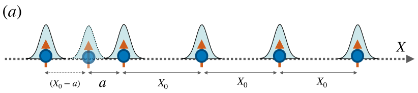
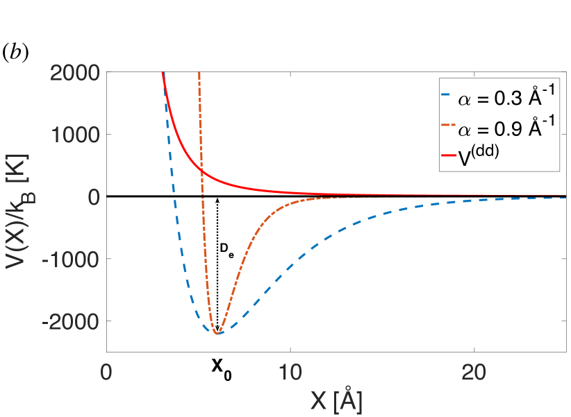
Figure 2: (a) Sketch of 1D molecular aggregate with off diagonal disorder, all transition dipoles are parallel. Shaded Gaussians indicate possible initial thermal position disorder of each monomer. (b) Inter-molecular potentials: Morse potential for $\alpha=0.3$ Å^-1 (blue dashed) and $\alpha=0.9$ Å^-1 (red dot-dashed) and the strength of dipole-dipole interactions $V_{nm}^{(dd)}$ (red solid line).

To be specific, we choose a mass $M=902330$ a.u. and a transition dipole moment $\mu=1.12$ a.u., such that nearest neigbor dipole-dipole interactions roughly match the real ones in e.g. carbonyl-bridged triaryl-amine (CBT) dyes Saikin et al. (2017).

III.1 Idealized adiabatic excitation transport

In this section, we first elucidate the concept of adiabatic excitation transport in a clear cut, albeit constructed case. For this, all molecules are initially placed at the equilibrium separation ($X_{0}=6$Å) of the Morse potential, except the first two molecules, which have a closer separation $a=4$Å, see Fig. 2 (a). For this configuration the dipole-dipole interaction between the first two molecules is much stronger than between any other neighboring molecules in the chain. This results in the localization of the excitation on these first two molecules, such that the initial electronic aggregate state is to a very good approximation the exciton

$$|\,{\psi(0)}\,\rangle=\frac{1}{\sqrt{2}}(|\,{m=1}\,\rangle+|\,{m=2}\,\rangle).$$ (12)

A second important consequence of the initial condition, is that the first two molecules very strongly repel each other, since they are deep on the inner repulsive side of the Morse potential in Fig. 2 (b). Around the geometry choice described so far, the initial positions and velocities of the molecules are randomized according to the Maxwell Boltzmann distribution foo at temperature $T=300$ K. However the standard deviation in position due to thermal motion is $0.5$ Å, which is fairly very small compared to the dislocation imposed on the first two sites i.e., 4 Å. Finally, we neglect on-site disorder in this section, such that $E_{m}=0$ in Eq. (II).

The resultant motion of the molecules and the excitation transfer are shown in Fig. 3, using Eq. (6) coupled to Eq. (9). Initially the two closest molecules strongly repel each other. Molecule 2 moves towards molecule 3, while molecule 1 escapes the chain, since the initial potential energy ${V}_{\mbox{\!\! \scriptsize 12}}^{(B)}(a)$ by far exceeds the binding energy $D_{e}$. When molecule 2 reaches molecule 3 those two constitute the new closest proximity pair. Since the motional time-scale ${\tau}_{\mbox{\!\! \scriptsize mov}}$ is large compared to the characteristic time-scale for dipole-dipole interactions $\tau_{dd}\equiv\pi/{V}_{\mbox{\!\! \scriptsize 12}}^{(dd)}(a)=2.7$ fs, the system can adiabatically follow the exciton quantum state that initially corresponds to Eq. (12), which is always localized on the two closest molecules. Around $t=0.5$ ps, it is hence now localized on molecule 2 and 3. Since in this close encounter, also the momentum is transferred from molecule 2 to molecule 3, the process continues along the chain until molecule 7 escapes it in the end. Just prior to that, at $t=2ps$ in Fig. 3, the excitation has to a large extent been transported to the end of the chain, on molecules 6 and 7.

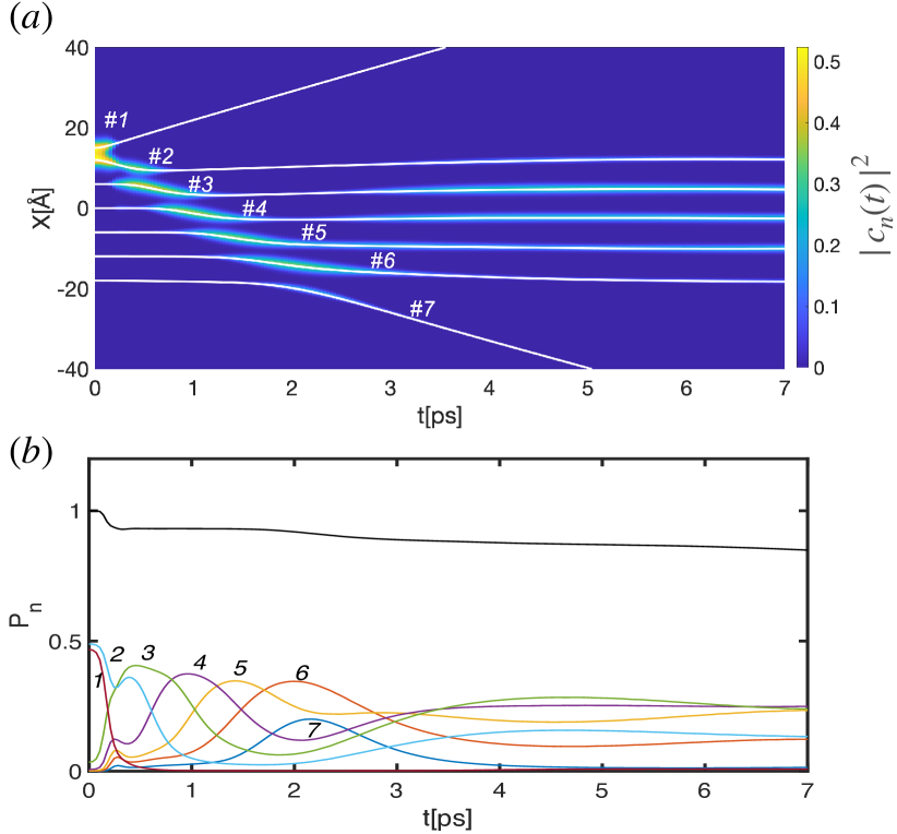
Figure 3: Exemplary adiabatic excitation transport with molecules. (a) (solid white) Mean trajectories of individual molecules, with site index $n$ as indicated. (color shading) Mean electronic excitation probabilities or diabatic populations $|c_{n}|^{2}$ are indicated by color around the respective trajectory. (b) (colored numbered lines) Individual diabatic populations $|c_{n}|^{2}$, (black solid) adiabatic population on the initial surface. Binding parameters are $\alpha=0.5$ Å^-1 and a well depth of $D_{e}=2200$ K. Results are averaged over $10^{5}$ trajectories.

We see a small change in the adiabatic population, black line in Fig. 3 (b), which reduces the transport fidelity. Otherwise, our extreme choice of initial conditions has replicated the near perfect transport scenario of the atomic case Wüster et al. (2010), where cold atoms are not bound to their neighbor. A very similar scenario arises if we start from the initially localized state $|\,{\psi(0)}\,\rangle=|\,{1}\,\rangle$. Since this can be written as a linear combination of (12) and the corresponding anti-symmetric exciton, both of which are adiabatically transported to the end of the chain as in Fig. 3, also the excitation from initial state $|\,{1}\,\rangle$ reaches the end of the chain through the motion.

In summary, a pulse combining motion and excitation transfer can facilitate high fidelity transport of an excitation through a chain. For its kinematic similarity with the popular class-room tool to demonstrate momentum conservation, the process has been likened to Newton’s cradle in Ref. Wüster et al. (2010). The physical basis is quantum adiabaticity, which leads to a limitation of this technique: To remain adiabatic, we require slow motion ${\tau}_{\mbox{\!\! \scriptsize mov}}\gg\tau_{dd}\equiv\pi/{V}_{\mbox{\!\! \scriptsize 12}}^{(dd)}(a)$, as discussed above, which means the transported excitation energy will always arrive earlier if we start in a localized state $|\,{\psi(0)}\,\rangle=|\,{\pi_{1}}\,\rangle$ instead of Eq. (12), and consider an equidistant chain. However, the situation is less clear when on-site energy disorder is present, since localization might then preclude an excitation starting in a localized state to arrive at all.

The example in this section has been chosen to clearly illustrate the concept of adiabatic excitation transport, but will not likely be practically useful due to the extreme and thus thermally inaccessible initial state for the positions of monomers 1 and 2. In the following we much more generally compare the transport properties of moving and static aggregates in the presence of on-site energy disorder.

III.2 Disorder and exciton localization

The on-site energy disorder $\sigma_{E}$ in an aggregate, sketched in Fig. 1 (b), arises due to the coupling of the monomers with their environment Wang et al. (2015); Adolphs and Renger (2006). Since the local environment may be different for each site, this can cause slightly different transition energy shifts $E_{n}$ for each monomer. We assume here that the time-scale for variation of such shifts is slow, so that the $E_{n}$ are constant throughout the transport process, hence we only treat static disorder. For the $E_{n}$ in Eq. (II), we assume a Gaussian distribution Valleau et al. (2012)

$$p_{E}(E_{n}-E_{0})=\frac{1}{\sqrt{2\pi\sigma_{E}}}e^{-(E_{n}-E_{0})^{2}/2\sigma_{E}}$$ (13)

where $\sigma_{E}$ is the standard deviation and $E_{0}$ the unperturbed transition energy of each molecule. The distribution is assumed to be identical for all monomers. For realistic systems, more sophisticated distributions may apply Eisfeld et al. (2010); Hestand and Spano (2018).

Disorder strongly affects the energy level structure and wave-function of exciton states in (4), which in turn influences the excitation transfer. One measure of the impact of disorder is the de-localization length of the exciton over the aggregate Meier et al. (1997); Ray and Makri (1999). For weak disorder the exciton is de-localized over the entire aggregate, while for strong disorder it becomes localized on a smaller number of monomers. This may cause exciton trapping Fidder et al. (1991, 1991), which is detrimental to excitation transport.

We now demonstrate that motion can help excitation transport overcome disorder induced localization in a simple test-case. For this, we take a chain composed of seven monomers placed at their equilibrium separations $X_{0}$, that are subject to thermal position and velocity distributions. We compare a static and a mobile scenario, both exhibiting an identical realisation of the disorder (13).

The dynamics of excitation transfer for a single trajectory without any initial close proximity of the first two molecules ($a=X_{0}$) is shown in Fig. 4. The disorder strength was $\sigma_{E}=500$ cm^-1, $\alpha=0.5$Å^-1 and the temperature $T=300$ K. At $t=0$ the excitation is injected at the first site (#1, input site), hence

$$|\,{\psi(0)}\,\rangle=|\,{m=1}\,\rangle.$$ (14)

in contrast to section III.1. We choose (14) for simplicity. Starting from this initial state, we investigate whether the excitation reaches the output site. We see that for the static system with $\dot{\mathbf{X}}=0$, the population reaching the output site remains very small Fig. 4(c). In contrast, for the dynamic system thermal fluctuations overcome the disorder and can deliver the excitation to the output site with quite high probability.

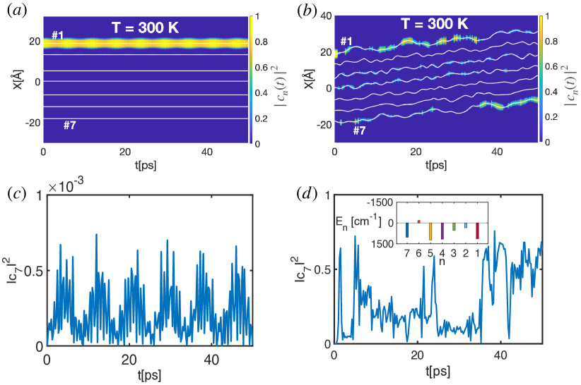
Figure 4: Excitation transport can overcome on-site energy disorder through motion. (a) Monomer trajectories and excitation probability in the immobile case in the same style as for Fig. 3. (b) The same for mobile molecules. (c) Population reaching the output site #7 in the immobile case. (d) The same for the mobile case. The inset shows the realisation of on-site energy disorder (13) used for both, panel (a) and (b).

While here we only demonstrated this for a specific single realisation of random positions, velocities and energy disorder, the latter shown in Fig. 4 (d), we will nextly confirm that motion can help to overcome disorder also in the ensemble average. A detailed inspection of the adiabatic populations $\tilde{p}_{n}=|\tilde{c}_{n}|^{2}$, see (7), shows however that the electronic dynamics is only intermittently adiabatic, with a large number of non-adiabatic transitions. We will comment on this again later in this article.

III.3 Transport efficiency

The single trajectory simulation in the previous section indicates that the motion of the molecules in an aggregate can potentially play a key role in transport of excitation energy in the presence of disorder. To explore this more deeply, we now quantify the efficiency of excitation transport at different temperatures $T$ and site disorders. We define the efficiency of excitation transfer $\epsilon_{\tau}$ in terms of the maximum probability for the excitation to reach to the output site within a time $\tau$, following e.g. Ref. Scholak et al. (2011):

$$\epsilon_{\tau}=\max_{t\in[0,\tau]}|\mbox{$\langle\,{m=\text{out}}\,|\,{\psi(t)}\,\rangle$}|^{2}.$$ (15)

The input site is #1 as in section III.2, and there is no initial dislocation $a=X_{0}$, besides disorder all molecules have the same mean distance from another.

For a given choice of molecular interaction potentials and temperature, we then calculate the mean efficiency by averaging over many different kinematic configurations with the initial positions and velocities of the molecules drawn from the Maxwell Boltzmann distribution as described in section III.1. We first calculate the maximum (15) for each realisation and then average these maxima over the trajectories. We finally compare two different efficiencies: $\epsilon_{\tau}^{(motion)}$, the transport efficiency in the case of mobile molecules and $\epsilon_{\tau}^{(static)}$, the transport efficiency in the case of immobile molecules. Note, that the latter case will still include position fluctuations according to a thermal distribution, only forces and velocities are set to zero.

The efficiency $\epsilon_{\tau}^{(motion)}$ is shown in Fig. 5 (a), after averaging over 5000 random configurations for seven sites, for the choice $\tau=50$ ps and output site #7. We consider a range of disorder strengths for which the aggregate transitions from de-localized excitons to strongly localized excitons for our choice of other parameters. We see that the effect of temperature on efficiency is small, within a reasonable range of temperature. This is because for the chosen $\alpha$, the accessible range of inter-molecular separations does not significantly vary with temperature due to the tight potential, see Fig. 2 (b). To assess the impact of motion on transport for any given case, we finally resort to the relative efficiency, defined as the ratio

$$\eta=\frac{\epsilon_{\tau}^{(motion)}}{\epsilon_{\tau}^{(static)}}.$$ (16)

For the same scenario, the relative efficiency $\eta$ is shown in Fig. 5 (b). In the chosen parameter range, we find relative efficiencies of up to about four, which indicates an enhanced transport in the mobile system compared to the static one.

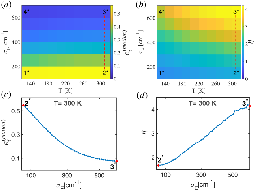
Figure 5: (a) Mean transport efficiency $\epsilon_{T}^{(motion)}$ averaged over 5000 trajectories, see Eq. (15), in the case of mobile molecules using a potential width according to $\alpha=0.5$Å^-1. Each of the $(6\times 10)$ tiles represents a simulation result for on-site disorder strength and temperatures indicated on the axes. Labels in the corners mark cases for which we show exemplary single trajectories in appendix B, Fig. 14. Large values of $\epsilon_{T}$ indicate a large probability to reach the output site from the input site. (b) Relative efficiency $\eta$ as the efficiency for the mobile scenario divided by the immobile one, see Eq. (16). In cases with $\eta>1$, the motion enhances transport, more so for higher values of $\eta$. Panels (c) and (d) show higher resolution 1D cuts along $\sigma_{E}$ indicated by the red lines in (a) and (b).

Nextly, we examine how this enhancement is affected by the width of the potential well that binds monomers to each other. The width is controlled by the parameter $\alpha$ in the Morse potential, (11). For small $\alpha$, the width of the well is increased, so we expect larger excursions of inter-molecular separations than for large $\alpha$. These may overcome the localization of excitons due to the accompanying strong variation of dipole-dipole interaction strengths. The efficiency for the mobile system is shown in Fig. 6 (a), single trajectories for the four parameter sets in the corners can be found in appendix B, Fig. 15. If the well is narrow, the transport efficiency remains smaller than for the case of wider well. This suggests, that larger dynamically accessible position deviations of the molecules enhance transport. Particularly for quite soft inter-molecular binding corresponding to $\alpha=0.3$ Å^-1 in Fig. 6, we see a marked impact of motion on excitation transport. Note however, that commonly encountered Morse potentials more typically correspond to $\alpha=0.8$ Å.

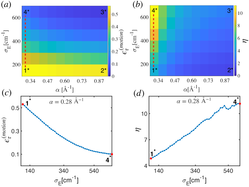
Figure 6: The same as for Fig. 5, but we vary the width of the inter-molecular binding potential well instead of the temperature, which is fixed at $T=300K$. Small $\alpha$ correspond to a larger width. Single trajectories for the labels in the corner of (a) are shown in appendix B, Fig. 15. Panels (c) and (d) show high resolution 1D cuts along $\sigma_{E}$ indicated by the red lines in (a) and (b). All results are averaged over $5000$ trajectories.

We have chosen the relatively small system size of 7 monomers for numerical convenience. Extending this to larger system of e.g. 13 molecules, we find that the relative efficiency $\eta$ increases with system size, for otherwise identical parameters. This is expected since the localisation length from energy disorder would remain constant, hence end-to-end transport without motion will be more strongly suppressed for larger chains. In contrast, the mode of adiabatic excitation transport as in Fig. 3 does not worsen much for larger chains, hence the relative improvement provided by motion could be larger. We have also considered more symmetric simulations with an excitation starting in the centre of the chain and exploring when it reaches either end, but allowing for an equal transport distance these are computationally more challenging and did not produce qualitatively different results.

III.4 Transport adiabaticity

While the motivation for the present work and the reason for our expectation that motion might aid transport stem from the concept of adiabatic excitation transport discussed in section III.1, the results shown so far indicate only that motion may have a beneficial effect, but not whether this is due to adiabatic processes. When looking at individual trajectories in more detail, which we show in appendix B, it appears that the quantum dynamics of the excitation contains both, adiabatic periods as well as non-adiabatic transitions. We however do find, that the parameter space regions with the largest relative efficiencies $\eta$, are more adiabatic than others, see appendix D.

To quantify a positive impact of adiabatic following of an exciton state on transport more precisely, we now employ the adiabaticity measure proposed in Pant and Wüster . Consider

$$t_{n}(t) =\sum_{k,k^{\prime}}\big{[}\left(\dot{\tilde{a}}_{k^{\prime}}(t)e^{-i\tilde{b}_{k^{\prime}}(t)}\>\tilde{c}_{k}(t)+\tilde{c}^{*}_{k^{\prime}}(t)\>\dot{\tilde{a}}_{k}(t)e^{i\tilde{b}_{k}(t)}\right)\>d^{(k)}_{n}(t)\>d^{(k^{\prime})*}_{n}(t)$$

$$+\tilde{c}^{*}_{k^{\prime}}(t)\>\tilde{c}_{k}(t)\>\left(\dot{d}^{(k)}_{n}(t)\>d^{(k^{\prime})*}_{n}(t)+d^{(k)}_{n}(t)\>\dot{d}^{(k^{\prime})*}_{n}(t)\right)\big{]},$$ (17)

$${T}_{\mbox{\!\! \scriptsize adiab}}(t) =\int_{0}^{t}dt^{\prime}\>\>{t}_{\mbox{\!\! \scriptsize out}}(t^{\prime}),$$ (18)

where $d^{(m)}_{n}(t)=\mbox{$\langle\,{n}\,|\,{\varphi_{m}(t)}\,\rangle$}$ is the component amplitude in basis state $|\,{n}\,\rangle$ for system eigenstate $|\,{\varphi_{m}(t)}\,\rangle$ and we have decomposed the adiabatic amplitude $\tilde{c}_{k}(t)$ in its polar representation $\tilde{c}_{k}(t)=\tilde{a}_{k}(t)e^{i\tilde{b}_{k}(t)}$, with $\tilde{a}_{k},\tilde{b}_{k}\in\mathbb{R}$.

As discussed in Pant and Wüster , (III.4) is obtained by taking the time-derivative of the population on a specific molecule $p_{n}(t)=|c_{n}(t)|^{2}$ and then removing the contribution due to beating between exciton eigen-states, which would also be present in the absence of motion. What remains is a measure for the site population change due to variations of the eigenstates. By construction, we have ${T}_{\mbox{\!\! \scriptsize adiab}}(t)=1$ at a time $t$ when the excitation has reached the output site such that this transfer was entirely due to adiabaticity. For further demonstrations and benchmarks we refer to Pant and Wüster .

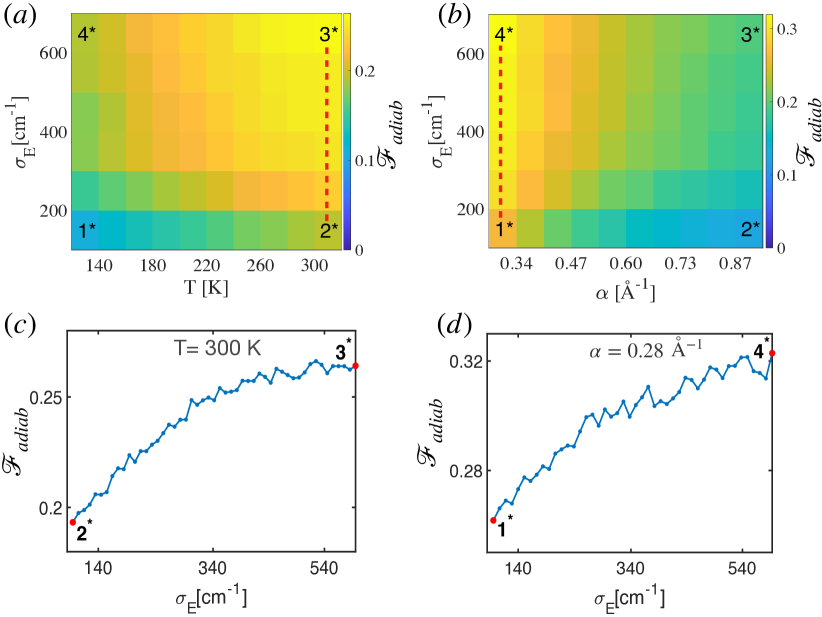
Figure 7: Quantification of transport adiabaticity. (a) Fractional adiabaticity ${\cal F}_{\mbox{\!\! \scriptsize adiab}}$ (defined in the text) for the same parameters as in Fig. 5 and in (b) corresponding to Fig. 6. Panels (c) and (d) show higher resolution 1D cuts along $\sigma_{E}$ indicated by the red lines in (a) and (b). All results are averaged over 5000 trajectories.

Let us define ${t}_{\mbox{\!\! \scriptsize max}}$ as the earliest time at which the population maximum is found on the output site, which then enters the transport efficiency evaluation (15). With this we finally define the fractional adiabaticity ${\cal F}_{\mbox{\!\! \scriptsize adiab}}={T}_{\mbox{\!\! \scriptsize adiab}}({t}_{\mbox{\!\! \scriptsize max}})/\epsilon_{\tau}$. We expect ${\cal F}_{\mbox{\!\! \scriptsize adiab}}$ to be of order unity if the transport is fully adiabatic, and to give an indication of the relative importance of adiabatic transport otherwise. We show ${\cal F}_{\mbox{\!\! \scriptsize adiab}}$ in Fig. 7 for the same parameters as Fig. 5 and Fig. 6. We see that parameter space regions with larger fractional adiabaticity roughly co-incide with those showing larger relative transport efficiencies. While this suggests a possible link between the efficiency of the transport and adiabatic motion of the molecules, note that the fractional adiabaticity magnitude remains relatively small.

IV Excitation transport by torsional motion

In the previous section, we have shown that while longitudinal motion of molecules along the aggregation direction can enhance the efficiency of excitation transport in the presence of disorder, this enhancement is not very large within the range of realistic parameters for molecular interaction, which are the narrowest potential explored by us. It turns out that the situation improves if the motional degree of freedom is changed from longitudinal motion to torsional motion, explored in this section. We now assume that the separation of the molecules is fixed at $3.4$ Å, but the molecules are allowed to rotate around the aggregate $X$-axis within the $YZ$-plane. Any possible relative tilt of the molecules out of this plane is ignored for simplicity.

The dipole-dipole interaction in Eq. (1) with these constraints can be written as

$${V}_{\mbox{\!\! \scriptsize mn}}^{(dd)}(\mathbf{\theta})=\frac{\mu^{2}}{X_{0}^{3}}\cos{\theta_{mn}},$$ (19)

where $\theta_{mn}=\theta_{n}-\theta_{m}$ is the angle between the direction of the transition dipole axes of molecule $m$ and molecule $n$, shown as red arrows in Fig. 8 (a). The transition dipole of magnitude $\mu$ is assumed spatially fixed in the plane of the molecule which can now rotate round the $X$-axis.

We assume that the molecules prefer to align at certain angles with their neighbors, which can be chemically engineered for example by the addition of appropriate side chains Haedler et al. (2015). To describe these preferred orientation and torsional excursions around them, we employ a potential energy

$${V}_{\mbox{\!\! \scriptsize mn}}^{(B)}(\mathbf{\theta}_{mn})=\frac{V_{0}}{2}[1-\cos{(2K_{\theta}(\theta_{mn}-\theta_{0}))}],$$ (20)

shown in Fig. 8 (b), where $V_{0}$ is the height of the potential barrier, $K_{\theta}$ determines the spacing of minima and hence the symmetry, and $\theta_{0}$ determines the equilibrium angle(s) and is fixed by the detailed shape of the molecule. For reasons that shall become clear shortly, we assume an approximate fourfold symmetry, hence $K_{\theta}=2$. The symmetry should not be perfect though, to justify the use of a single excited electronic state per molecule, and hence a well defined direction for the transition dipole moment.

In order to allow the potential (20) to control equilibrium orientations of the molecules, and not be overwhelmed by a torque from dipole-dipole interactions in (19), we have changed the dipole strength to $\mu=0.6$ a.u., which is about half of the value taken in section III for longitudinal motion.

After fixing the desired symmetry, we nextly adjust the torsional potential strength $V_{0}$ such that the angular spread $\Delta\theta$ in thermal equilibrium at $T=300$K is $\Delta\theta=8^{\circ}$, roughly matching angular spreads modelled in Ref. Saikin et al. (2017). This results in the maximum value of the potential $V_{0}/k_{B}=1923K$. While this potential in principle still allows full rotations of the molecules, near room temperature molecules will almost exclusively perform small torsional oscillations about the minima of (20).

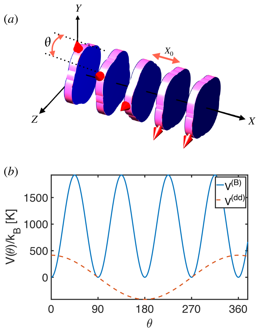
Figure 8: (a) Sketch of the central units in a 1D self-assembled chain of dyes, which can slightly rotate about the aggregation axis. (blue disk) molecules, (red arrow) direction of the transition dipole moment between $|\,{g}\,\rangle$ and $|\,{e}\,\rangle$. (b) (solid blue line) Periodic potential (20) for the torsional motion of the molecules in (a), with a periodicity of $90^{\circ}$ due to some assumed approximate four-fold symmetry of each molecule. (red dashed) Strength of dipole-dipole interactions (19) for orientation.

We model torsional dynamics analogous to the case of longitudinal motion, except that instead of the positions $X_{n}$, the angles $\theta_{n}$ are allowed to evolve. The classical equations of motion for the angular displacement of molecules read

$$I\frac{\partial^{2}}{\partial t^{2}}{\theta}_{m}=-\nabla_{{\theta}_{m}}U_{s}({\theta})-\sum_{n}\nabla_{{\theta}_{m}}V_{mn}^{(B)}.$$ (21)

See appendix A for the our simple estimate of a representative moment of inertia $I$ for dye molecules, based on CBT. As before, the exciton dynamics is obtained by expanding the total wavefunction in diabatic states

$$i\frac{\partial}{\partial t}{c}_{m}=\sum_{n=1}^{N}H_{mn}[\mathbf{\theta}_{mn}(t)]{c}_{n},$$ (22)

where $H_{mn}[\mathbf{\theta}_{mn}(t)]$ is the matrix element for the electronic coupling in Eq. (II), with dipole-dipole interaction given by Eq. (19).

IV.1 Idealized adiabatic excitation transport

As in section III.1, we begin with the basic demonstration that molecular torsion can cause transport in principle. We assume that the orientations of all molecules are at the equilibrium of the torsional potential Eq. (20), with angle between adjacent axes of $\theta_{0}=70^{\circ}$. Now if we decrease the angular separation between the direction of the dipole moments of first two molecules the dipole-dipole interaction between these two molecules is stronger and the excitation will again get localised on them as in (12). The angular distribution and the angular velocity distribution of each monomer is again a Gaussian with standard deviation $\sigma_{\theta}$ and $\sigma_{\omega}$ respectively, disorder is set to zero, $E_{m}=0$. Similar to section III.1, the standard deviation in angular position ($\sigma_{\theta}=8^{\circ}$) is small compared to the angular offset between the first two molecules ($\Delta{\theta}=30^{\circ}$). The dynamics of excitation transport is now obtained by solving Eq. (21) and Eq. (22) as a coupled system.

The resultant excitation transport is show in Fig. 9, averaged over $10^{5}$ trajectories. The dislocation at the end will cause a repulsive torque on molecule 2 which causes it to rotate its axis towards that of molecule 3, increasing the dipole-dipole interaction between those two and carrying the excitation with it, as in section III.1. Again the scheme proceeds over several sites.

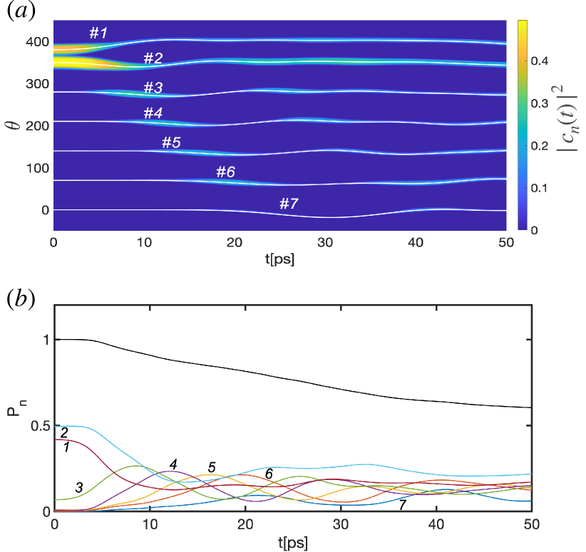
Figure 9: Exemplary adiabatic excitation transport by molecular rotations. (a) (solid white) Mean orientation angles of individual molecules, with site index $n$ as indicated. (color shading) Mean electronic excitation probabilities or diabatic populations $|c_{n}|^{2}$ are indicated by color around the respective trajectory. (b) (colored numbered lines) Individual diabatic populations $|c_{n}|^{2}$, (black solid) adiabatic population on the initial surface. Results are averaged over $10^{5}$ trajectories.

Compared to the scenario of section III.1, we see a larger reduction of adiabatic population as the black line in Fig. 9 (b), with a corresponding larger drop of the fidelity of transport.

IV.2 Transport efficiency

In this section we explore to what extent torsional motion of the molecules during energy transport can overcome disorder. We again take a chain of seven molecules, however now assume orthogonal dipole moment axes of adjacent molecules, i.e. $\theta_{0}=\pi/2$ in Fig. 8 (a). We chose this angle since dipole-dipole interactions at the precise equilibrium position vanish, which will necessarily enhance the relative impact of random molecular rotations near the equilibrium orientation on dipole-dipole interactions and hence exciton states.

Fluctuations of on-site-energies are again described by Eq. (13). The transport of excitation for a single trajectory at room temperature for both, the mobile and the static system is shown in figure Fig. 10. As in section III.2 the initial state of excitation at time $t=0$ is $|\,{\Psi(0)}\,\rangle=|\,{1}\,\rangle$. The standard deviation for orientation angles at room temperature is taken to be $\sigma_{\theta}=8^{\circ}$. We see as in section III.2, that in a case where for the static system the excitation is almost completely localized on the input site, the mobile system manages to transfer 80% of the excitation energy to the output site. Therefore also torsional motion of the molecules can help to combat localization and guide the transfer of excitation along the chain.

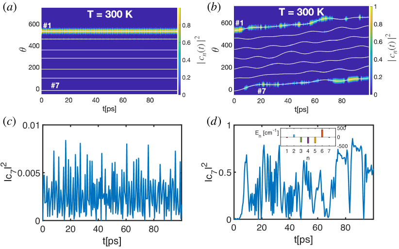
Figure 10: Excitation transport through torsional motion can overcome disorder. (a) Monomer orientations and excitation probability in the immobile case in the same style as for Fig. 3. (b) The same for mobile molecules. (c) Population reaching the output site #7 in the immobile case. (d) The same for the mobile case. The inset in (d) shows the selected single realisation of on-site energy disorder.

The effect of site disorder and temperature on efficiencies and relative efficiencies is shown in Fig. 11, using the same definitions as in section III.3. Here the potential (20) is fixed and the efficiency is obtained by averaging over 5000 random configurations of seven sites. We have re-adjusted the range of disorder strengths to cover the regime from de-localized excitons to strongly localized excitons for the different setting here. In contrast to results in section III.3, there is now a small increase in efficiency with temperature for the mobile system. We see an even more significant increase in the relative transport efficiency Fig. 11b, compared to the case of longitudinal motion.

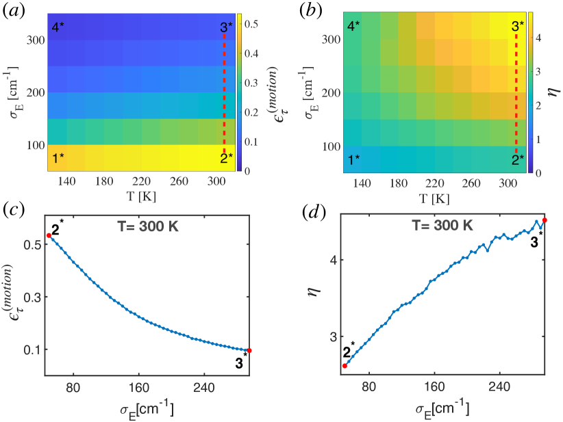
Figure 11: Variation of transport efficiency with disorder strength and temperature for torsional motion of molecules, for a well width of $\sigma_{\theta}=8^{\circ}$. (a) Absolute efficiency $\epsilon_{T}^{(motion)}$ in the mobile case. Labels in the corners mark cases for which we show exemplary single trajectories in appendix C, Fig. 17. (b) Relative efficiency $\eta$ as the efficiency for the mobile scenario divided by the immobile one. Panels (c) and (d) show higher resolution 1D cuts along $\sigma_{E}$ indicated by the red lines in (a) and (b). The results are averaged over $5000$ trajectories.

Nextly, we fix the temperature at $T=300$ K and vary the width of the potential well by changing $V_{0}$ in the potential (20) and hence $\sigma_{\theta}$. The results are shown in Fig. 12.

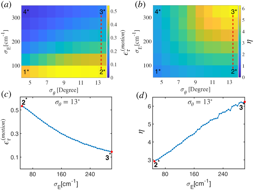
Figure 12: Variation of transport efficiency with disorder strength and well width for torsional motion of molecules at $T=300$ K. (a) Absolute efficiency $\epsilon_{T}^{(motion)}$ in the mobile case. Labels in the corners mark cases for which we show exemplary single trajectories in appendix C, Fig. 18. (b) Relative efficiency $\eta$ as the efficiency for the mobile scenario divided by the immobile one. Panels (c) and (d) show higher resolution 1D cuts along $\sigma_{E}$ indicated by the red lines in (a) and (b). The results are averaged over $5000$ trajectories.

As in the earlier section on longitudinal motion, we recover the scheme that wider potentials allowing a larger range of motion give rise to larger relative efficiencies of excitation transport.

IV.3 Transport adiabaticity

An inspection of the adiabaticity of individual trajectories, shown in appendix C, again shows a mixture of adiabatic and non-adiabatic contributions to the dynamics, as we had seen for the scenario with longitudinal motion along the aggregate axis. We also again find the general trend that regions in parameters space with high relative efficiency co-incide with those showing more adiabaticity, see appendix D.

The same quantification ${\cal F}_{\mbox{\!\! \scriptsize adiab}}$ of the relevance of adiabaticity for the enhancement of quantum transport through motion that we discussed in section III.4 is shown in Fig. 13 for the case of torsional motion of monomers. Similar to our results for longitudinal motion, the fractional adiabaticity is large in the regime where the relative efficiency is large, suggesting a link of the increase in the efficiency of the transport and adiabatic rotation of the molecules.

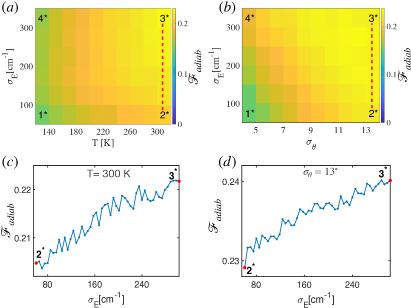
Figure 13: Quantification of transport adiabaticity. (a) Fractional adiabaticity ${\cal F}_{\mbox{\!\! \scriptsize adiab}}$ (defined in section III.4) for the same parameters as in Fig. 11. (b) Corresponding to Fig. 18. Panels (c) and (d) show higher resolution 1D cuts along $\sigma_{E}$ indicated by the red lines in (a) and (b). The results are averaged over 5000 trajectories.

V Conclusions and outlook

We have explored how mechanical motion of the molecules in an aggregate affects the efficiency of excitation transport compared to an immobile scenario. We find a motion-induced enhancement of the excitation transfer efficiency over static configuration in the presence of on-site energy disorder for both, longitudinal motion of molecules along the aggregate axis and rotational or torsional motion of them in the plane orthogonal to that axis, in small systems of up to $N=7$ monomers. We conclude that a strong connection between the motion of the molecules and the propagation of the electronic excitation has the potential to increase the efficiency of excitation transfer significantly, in cases where the coupling to internal molecular vibrations can be neglected.

We separately simulated longitudinal motion of monomers along the aggregation axis and torsional motion in a plane orthogonal to that axis, and found that the torsional mode will have more beneficial impact on transport due to larger variations in interaction strengths that are realistically accessible. Additional simulations involving both torsional and translational degrees of freedom show qualitatively unchanged results compared to those presented here.

While a possible cause of enhancement of transport can be found in adiabatic excitation transport Wüster et al. (2010) as demonstrated in section III.1 and section IV.1, for most of the inspected parameter space the situation is less clear, with dynamics exhibiting both: periods where eigenstates are adiabatically followed, interspersed with sudden non-adiabatic transitions. For electronic dynamics involving superpositions of excitons and thus transport from site to site also in the absence of any motion, a clear link between transport and adiabaticity or its absence is difficult to establish. To nonetheless quantify the importance of adiabaticity for the motional enhancement of transport, we have employed the adiabaticity measure proposed in Pant and Wüster . We find that adiabatic contributions are significant but not likely crucial for transport enhancement, but regions of high adiabaticity co-incide with those showing efficient transport.

In this article, we have ignored the effect of intramolecular vibrations in excitation transport, although these frequently play a crucial role in transport Caruso et al. (2009); Ritschel et al. (2015); Roden et al. (2009); Ritschel et al. (2011); Roden et al. (2012); Qin et al. (2014); Ai and Zhu (2012); Olaya-Castro et al. (2008); Liang (2010); Ghosh et al. (2011). In the next step of this exploration, we will thus extend the quantum dynamics calculation for excitation transport to an open-quantum-system technique, such as non-Markovian quantum state diffusion Suess et al. (2014); Diósi and Strunz (1997); Diósi et al. (1998); Roden et al. (2009), which will be coupled to classical time-dependent trajectory for the molecules as in this work. Earlier research using simpler models for motion and energy disorder than the present work suggests that motion can enhance transport even in the presence of decohering environments Asadian et al. (2010); O‘Reilly and Olaya-Castro (2014).

Another significant extension to bridge the gap between these model calculations and realistic molecular systems, would be to treat energy transport beyond the dipole-dipole approximation. For the relevant case where the intermolecular distance is comparable to the size of the molecules, higher multipole transitions play a significant roleKrueger et al. (1998); Nasiri Avanaki et al. (2018); Craig and Thirunamachandran (1998). Short range excitonic couplings may significantly deviate from the dipolar form showing an exponential distance dependence Madjet et al. (2009). Since adiabatic transport discussed here relies on significant changes of the excitonic Hamiltonian with molecular positions, it might be enhanced by such effects.

For a final confirmation for realistic and technologically relevant settings, such as dye-sensitised light harvesting technology Zhang and Cole (2017); Ghosh and Feng (1978), we can replace the simple classical point particle motion of the present article (6) by full fledged molecular dynamics simulations evolving all the nucleii, and the evolution of electronic states by the simple matrix model (9) used here with time-dependent density functional theory of the many electron aggregate system in what is known as QM-MM schemes. Such studies could then confirm whether adiabatic or motion-induced enhanced transport is an effective countermeasure to exciton trapping. Alternatively even the full quantum dynamics of the system might be tractable using multiconfigurational techniques such as the multi-layer multiconfiguration time-dependent Hartree (ML-MCTDH) method Binder and Burghardt (2019).

Finally, since this work was inspired by ideas that have originated in a quantum simulation context with cold atoms Wüster et al. (2010), also other features discovered in that context might be portable to a molecular setting. One prominent one is the use of conical intersections Yarkony (2001) as switches for coherence and direction of excitation transport Leonhardt et al. (2014, 2016, 2017).

Conflicts of interest

There are no conflicts to declare.

Appendix A Estimate of dye-molecule moment of inertia and rotational potential

For example, in the supramolecular assembly of Ref. Haedler et al. (2015) that provided some guidance for our simple model of torsional motion in section IV, a single monomer consist of a CBT core attached via amide linker with 4-(5-hexyl-2,$2^{\prime}$-bithiophene)naphtalimide (NIBT). Therefore the total mass of the monomer is the sum of masses of these constituents, which amounts to $M=1009.03$ amu. We simply assume that this mass is distributed uniformly in a square disc, with side length $a=50$ Å. The moment of inertia of a disc with mass density $\rho$ is

$$I=\frac{1}{6}\rho a^{4}.$$ (23)

For a uniform mass distribution $\rho=M/(a^{2})$ we then find a moment of inertia of $2.95\times 10^{9}$ a.u.

The maximum of the potential barrier $V_{0}$ is obtained by taking the Taylor expansion of Eq. (20) about $\theta_{mn}=\theta_{0}$, and then defining a target angular width $\Delta\theta$ using the thermal equipartition theorem

$$V_{0}K_{\theta}(\Delta\theta)^{2}=\frac{k_{B}T}{2}.$$ (24)

We assume a typical angular spread $\Delta\theta=8^{\circ}$ at temperature $300K$ similar to Ref. Saikin et al. (2017), from which we obtain ${V_{0}}/{k_{B}}=1923K$.

To obtain $\sigma_{\theta}$ at a different temperature T after this initial allocation, we again use Eq. (24), $\sigma_{\theta}=\sqrt{\frac{k_{B}T}{2K_{\theta}V_{0}}}$. The distribution in angular velocity also relies on the equipartition theorem, yielding a width $\sigma_{\omega}=\sqrt{k_{B}T/I}$.

Appendix B Single trajectories for longitudinal motion

To provide more intuitive access to the ensemble averaged results in the main text, section III.3, we now additionally provide some individual trajectories along the edges of the investigated parameter space.

We see in the bottom panels (1* and 2*) of Fig. 14, that for small energy disorder $\sigma_{E}$, the localization effect is weak. Thus even in the absence of molecular motion the excitation quite likely and rapidly reaches the output site, a result that no longer can be much improved upon by motion. In contrast, the upper panels (3* and 4*) with strong disorder show quite localised excitons, where for example panel #3 then shows dynamics where this disorder has been overcome by thermal motion.

Table 1: Parameters for single trajectory data in Fig. 14. Positions refer to the tags in Fig. 5

. Positions Parameters $\#1$ $\sigma_{E}=100$ $cm^{-1}$ and $T=120$ $K$ $\#2$ $\sigma_{E}=100$ $cm^{-1}$ and $T=300$ $K$ $\#3$ $\sigma_{E}=600$ $cm^{-1}$ and $T=300$ $K$ $\#4$ $\sigma_{E}=600$ $cm^{-1}$ and $T=120$ $K$

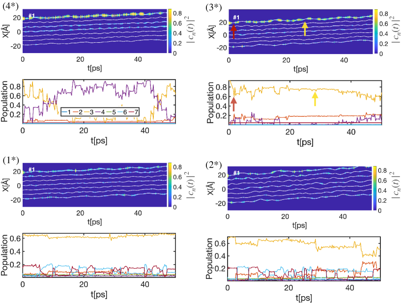
Figure 14: Single trajectory time evolution of the position of individual molecules together with exciton dynamics for $\alpha=0.5$ Å^-1. The numbering refers to tags in Fig. 5 and the four different parameter sets given in table 1. Top panels show molecular coordinates and diabatic populations $|c_{n}(t)|^{2}$ in the same style as Fig. 3 (a). Bottom panels show the corresponding adiabatic populations $|\tilde{c}_{n}(t)|^{2}$, with legend included for case (4^∗). Surfaces are numbered from the highest energy exciton state to the lowest. Colored arrows refer to specific dynamical events discussed in the text.

By controlling the width of the inter-molecular binding well, we can control the amplitude of excursions of the molecules. Single trajectories here show how the probability of excitation transport is influenced by changing the width as well as the site disorder. We see in Fig. 15 that even for large site disorder the excitation energy can reach the output site with probabilities of more than $50\%$ in the mobile case.

Table 2: Parameters for single trajectory data in Fig. 15. Positions refer to the tags in Fig. 6

Positions	Parameters
$\#1$	$\sigma_{E}=100$ $cm^{-1}$ and $\alpha=0.30$ Å-1
$\#2$	$\sigma_{E}=100$ $cm^{-1}$ and $\alpha=0.87$ Å-1
$\#3$	$\sigma_{E}=600$ $cm^{-1}$ and $\alpha=0.87$ Å-1
$\#4$	$\sigma_{E}=600$ $cm^{-1}$ and $\alpha=0.30$ Å-1

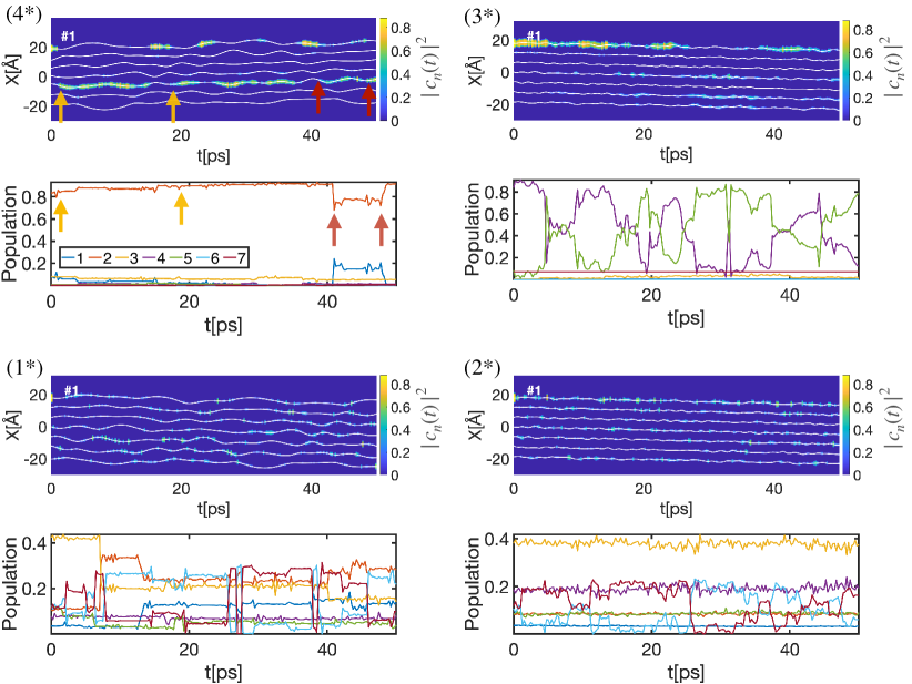
Figure 15: Single trajectory time evolution of the position of individual molecules together with excitation dynamics, in the same style as Fig. 14, but here we fix the temperature at $300K$. The numbering refers to tags in Fig. 6 and the four different parameter sets given in table 2. Colored arrows refer to specific dynamical events discussed in the text.

Further analysis of adiabatic populations reveals that the exciton dynamics is rarely purely adiabatic but typically shows frequent non-adiabatic transitions. To assess these further, we show adiabatic populations for the trajectories in Fig. 14 and Fig. 15. From these we can deduce that the evolution shows a mixture of two types of dynamics: Firstly adiabatic periods, during which adiabatic populations $|\tilde{c}_{n}(t)|^{2}$ stay nearly constant. Secondly, prominent intermittent non-adiabatic transitions, at which adiabatic populations show quite sudden significant changes. If we manually relate either of these two features in the bottom panels with the excitation probability of each molecule shown in the top panels, we can identify two manifestations of adiabatic transport that differ in clarity: (i) During a period of adiabaticity, the excitation exhibits a slow transfer from one molecule to another, see Fig. 15 panel (4*), at times indicated by yellow arrows near $t=2$ ps and $t=19$ ps. This clearly corresponds to adiabatic transport as discussed in section III.1. (ii) Exactly coinciding with a sudden partial non-adiabatic transition, the excitation transfers from one molecule to another, see Fig. 15 panel (4*), around $t=42$ ps and $t=48$ ps, marked with red arrows. Here one might suspect non-adiabatic excitation transport. A detailed inspection of the evolution of the involved eigenstates, shown in Fig. 16, however shows that transport is due to the fraction of population that remains in the same eigenstate. We thus still see adiabatic excitation transport, albeit with an efficiency reduced by the concurrent non-adiabatic transition.

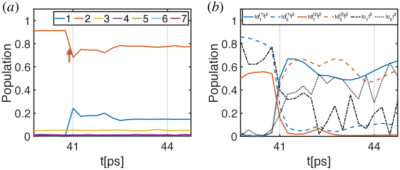
Figure 16: Only partially adiabatic transport. We show a zoom onto a red arrow in Fig. 15 panel (4*) between $t=40$ ps and $t=44$ ps. (a) Adiabatic populations (b) The two relevant site-populations $d^{(m)}_{n}(t)=\mbox{$\langle\,{n}\,|\,{\varphi_{m}(t)}\,\rangle$}$ for the two dominant excitons, see legend. We also show the total population on sites 1 and 5.

Appendix C Single trajectories for torsional motion

Similar to the longitudinal motion scenario, we now illustrate the effect of temperature and site disorder on excitation transport with individual simulation trajectories, but fixing the molecular positions and allowing instead a rotation of the molecular transition dipole axes.

Fig. 17 shows the single trajectories at different temperatures for fixed width of the torsional potential well. When the energy disorder is small, for example in the bottom panels of Fig. 17, the localization effect is weak and similar to the case with longitudinal motion the excitation rapidly reaches the output site with high arrival probability even in the absence of motion. In contrast, once we increase the energy disorder towards the upper panels, the excitation is more localized in the immobile system. Then, for the mobile system we see a clear transport of the exciton to the output site.

Table 3: Parameters for single trajectory plots in Fig. 17. Positions refer to the tags in Fig. 11

Positions	Parameters
$\#1$	$\sigma_{E}=100$ $cm^{-1}$ and $T=120$ $K$
$\#2$	$\sigma_{E}=100$ $cm^{-1}$ and $T=300$ $K$
$\#3$	$\sigma_{E}=300$ $cm^{-1}$ and $T=300$ $K$
$\#4$	$\sigma_{E}=300$ $cm^{-1}$ and $T=120$ $K$

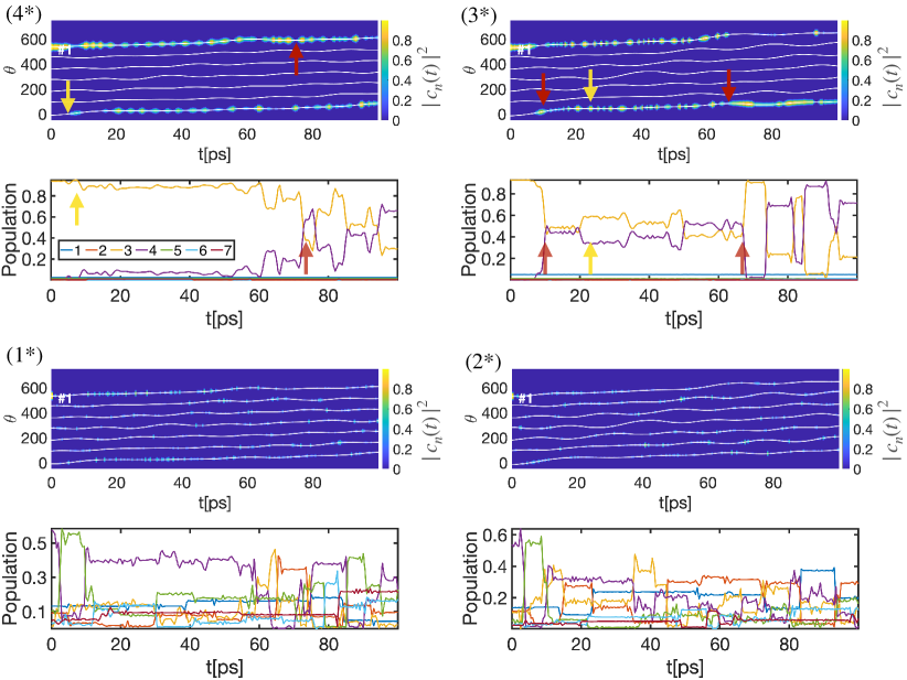
Figure 17: Single trajectory time evolution of the angular position and exciton dynamics for $\sigma_{\theta}=8^{\circ}$. The numbering refers to tags in Fig. 11 (a) and the four different parameter sets given in table 3. Even for large site disorder the excitation energy transfer to the output site is clearly seen. Colored arrows refer to specific dynamics events discussed in the text.

Nextly, we provide single trajectories for different widths of the potential in Fig. 18. For wide wells (panel #3) and high on-site disorder, when almost $90\%$ of the exciton is localized on the first site for immobile molecules, we see that the excitation is reaching the output site with more than $80\%$ probability if motion is included.

Table 4: Parameters for single trajectory plots in Fig. 18. Positions refer to the tags in Fig. 12

Positions	Parameters
$\#1$	$\sigma_{E}=100$ $cm^{-1}$ and $\sigma_{\theta}=4^{\circ}$
$\#2$	$\sigma_{E}=100$ $cm^{-1}$ and $\sigma_{\theta}=13^{\circ}$
$\#3$	$\sigma_{E}=300$ $cm^{-1}$ and $\sigma_{\theta}=13^{\circ}$
$\#4$	$\sigma_{E}=300$ $cm^{-1}$ and $\sigma_{\theta}=4^{\circ}$

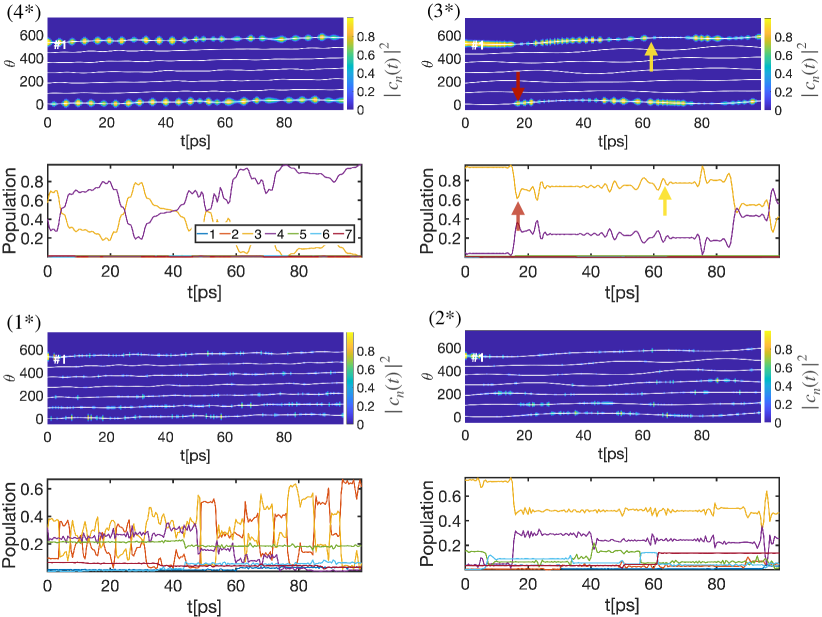
Figure 18: Single trajectory time evolution of the angular position and exciton dynamics similar to Fig. 17, but here we fix the temperature at $300K$. The numbering refers to tags in Fig. 12 (a) and the four different parameter sets given in table 4. We can see a clear transport of excitation even for large site disorder. Colored arrows refer to specific dynamics events discussed in the text.

As in the case of longitudinal transport, we see a mixture of clear cut adiabatic transport processes and others impeded by a concurrent non-adiabatic transition. A relatively clear trajectory containing both is shown in Fig. 18 panel (3^∗): The evolution is non-adiabatic near $20$ ps but then it is fairly adiabatic from $20$ to $85$ ps. Exactly at the moment of non-adiabaticity, the top panel shows how the excitation migrated from molecule 1 to molecule 7, due to the fraction of the population that has not changed state. Fast oscillations in diabatic populations can be attributed to beating from a superposition of exciton states, created by the non-adiabatic transition. However note the longer time scale variations which shifts most of the excitation probability back from site 7 to site 1 around $t=25$ ps and then back again around $t=45$ ps. Neither event is accompanied by a significant change in adiabatic populations, hence we would classify these changes as adiabatic transport.

Appendix D Survey of adiabaticity

The relative adiabaticity measure ${\cal F}_{\mbox{\!\! \scriptsize adiab}}$ introduced in section III.4 provides a measure of adiabatic transport. The less ambitious goal of quantifying the global level of adiabaticity (regardless of whether it leads to transport or not) in different regions of parameter space can be gained from our quantum-classical propagation algorithm itself and is presented in this appendix.

The molecules move on a single adiabatic potential energy surface $m$, which may be changed via sudden jumps to another surface $n$ by non-adiabatic couplings Eq. (8) between surface $m$ and surface $n$. A simple estimate of non-adiabaticity is thus provided by the mean number of allowed jumps Tully (1990); Hammes-Schiffer and Tully (1994); Möbius et al. (2011). The mean number of jumps per trajectory is shown for longitudinal motion in Fig. 19 and for torsional motion in Fig. 20, for the same two cuts through parameter space discussed in the main article. We find a larger number of jumps at high temperatures or narrow width of the potential well. This is expected since either involve faster motion of molecules, which directly increases all non-adiabatic couplings in Eq. (8). When we compare Fig. 19 with Fig. 5 and Fig. 6, we find that regions of high relative efficiency coincide with those of less allowed jumps and thus more adiabatic dynamics.

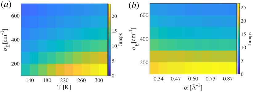
Figure 19: Mean number of allowed surface jumps in Tully’s algorithm, corresponding to non-adiabatic transitions, for longitudinal motion. (a) We vary temperatures and on-site disorder strengths. (b) We vary the width of the inter-molecular binding potential well and on-site disorder strengths.

Similar conclusions can be drawn from for the case of torsional motion in Fig. 20. For narrow width of the potential well or high temperature, the number of allowed jumps is large due to the faster angular vibration of molecules. In contrast, there are fewer jumps when we decrease temperature or increase the width of the well or on-site disorder strength. Again, in the region of high relative efficiency in Fig. 11 and Fig. 12 the transport is more adiabatic than in other regions.

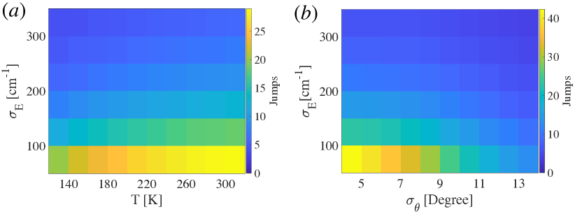
Figure 20: Mean number of allowed jumps similar to Fig. 19 for torsional motion. (a) For different temperatures and (b) for different widths of the well, as well as in both cases varied energy disorder strength.

The results in this appendix point in the same direction as those in section III.4 and section IV.3, where we show that parameter space regions where motion improves transport co-incide with higher adiabatic contributions to that transport.

References

- Brixner et al. (2017) T. Brixner, R. Hildner, J. Köhler, C. Lambert and F. Würthner, Advanced Energy Materials, 2017, 7, 1700236.
- Haedler et al. (2016) A. T. Haedler, S. C. Meskers, R. H. Zha, M. Kivala, H.-W. Schmidt and E. Meijer, Journal of the American Chemical Society, 2016, 138, 10539–10545.
- van Amerongen et al. (2000) H. van Amerongen, L. Valkunas and R. van Grondelle, Photosynthetic Excitons, World Scientific, Singapore, 2000.
- van Grondelle and Novoderezhkin (2006) R. van Grondelle and V. I. Novoderezhkin, Phys. Chem. Chem. Phys., 2006, 8, 793.
- Zhang and Cole (2017) L. Zhang and J. M. Cole, Journal of Materials Chemistry A, 2017, 5, 19541–19559.
- Ghosh and Feng (1978) A. K. Ghosh and T. Feng, Journal of Applied Physics, 1978, 49, 5982–5989.
- Malyshev et al. (2000) V. A. Malyshev, H. Glaeske and K.-H. Feller, The Journal of Chemical Physics, 2000, 113, 1170–1176.
- Saikin et al. (2013) S. K. Saikin, A. Eisfeld, S. Valleau and A. Aspuru-Guzik, Nanophotonics, 2013, 2, 21–38.
- Macedo et al. (2019) A. G. Macedo, L. P. Christopholi, A. E. Gavim, J. F. de Deus, M. A. M. Teridi, A. R. bin Mohd Yusoff and W. J. da Silva, Journal of Materials Science: Materials in Electronics, 2019, 1–22.
- Wüster and Rost (2018) S. Wüster and J. M. Rost, Journal of Physics B: Atomic, Molecular and Optical Physics, 2018, 51, 032001.
- Schönleber et al. (2015) D. Schönleber, A. Eisfeld, M. Genkin, S. Whitlock and S. Wüster, Physical review letters, 2015, 114, 123005.
- Hague and MacCormick (2012) J. Hague and C. MacCormick, New Journal of Physics, 2012, 14, 033019.
- Kasha (1963) M. Kasha, Radiation research, 1963, 20, 55–70.
- Chen and Silbey (2011) X. Chen and R. J. Silbey, The Journal of Physical Chemistry B, 2011, 115, 5499–5509.
- Roden et al. (2009) J. Roden, A. Eisfeld, W. Wolff and W. T. Strunz, Physical review letters, 2009, 103, 058301.
- Haken and Reineker (1972) H. Haken and P. Reineker, Zeitschrift für Physik, 1972, 249, 253–268.
- Barredo et al. (2015) D. Barredo, H. Labuhn, S. Ravets, T. Lahaye, A. Browaeys and C. S. Adams, Phys. Rev. Lett., 2015, 114, 113002.
- Labuhn et al. (2016) H. Labuhn, D. Barredo, S. Ravets, S. de Léséleuc, T. Macrì, T. Lahaye and A. Browaeys, Nature, 2016, 534, 667–670.
- Marcuzzi et al. (2017) M. Marcuzzi, J. c. v. Minář, D. Barredo, S. de Léséleuc, H. Labuhn, T. Lahaye, A. Browaeys, E. Levi and I. Lesanovsky, Phys. Rev. Lett., 2017, 118, 063606.
- Wüster et al. (2010) S. Wüster, C. Ates, A. Eisfeld and J. Rost, Physical review letters, 2010, 105, 053004.
- Möbius et al. (2011) S. Möbius, S. Wüster, C. Ates, A. Eisfeld and J. Rost, Journal of Physics B: Atomic, Molecular and Optical Physics, 2011, 44, 184011.
- Roden et al. (2009) J. Roden, G. Schulz, A. Eisfeld and J. Briggs, The Journal of chemical physics, 2009, 131, 044909.
- Roden et al. (2012) J. Roden, W. T. Strunz, K. B. Whaley and A. Eisfeld, The Journal of chemical physics, 2012, 137, 204110.
- Eisfeld and Briggs (2002) A. Eisfeld and J. S. Briggs, Chemical Physics, 2002, 281, 61–70.
- Haedler et al. (2015) A. T. Haedler, K. Kreger, A. Issac, B. Wittmann, M. Kivala, N. Hammer, J. Köhler, H.-W. Schmidt and R. Hildner, Nature, 2015, 523, 196.
- Kang et al. (2019) S. Kang, C. Kaufmann, Y. Hong, W. Kim, A. Nowak-Król, F. Würthner and D. Kim, Structural Dynamics, 2019, 6, 064501.
- (27) R. Pant and S. Wüster, 2020,https://arxiv.org/abs/2007.10707.
- Asadian et al. (2010) A. Asadian, M. Tiersch, G. G. Guerreschi, J. Cai, S. Popescu and H. J. Briegel, New J. Phys., 2010, 12, 075019.
- Semiao et al. (2010) F. Semiao, K. Furuya and G. Milburn, New Journal of Physics, 2010, 12, 083033.
- Behzadi and Ahansaz (2017) N. Behzadi and B. Ahansaz, International Journal of Theoretical Physics, 2017, 56, 3441–3451.
- O‘Reilly and Olaya-Castro (2014) E. J. O‘Reilly and A. Olaya-Castro, Nature communications, 2014, 5, 3012.
- Mülken and Bauer (2011) O. Mülken and M. Bauer, Physical Review E, 2011, 83, 061123.
- Binder et al. (2018) R. Binder, D. Lauvergnat and I. Burghardt, Physical review letters, 2018, 120, 227401.
- Binder and Burghardt (2019) R. Binder and I. Burghardt, Faraday discussions, 2019, 221, 406–427.
- Stier and Prezhdo (2002) W. Stier and O. V. Prezhdo, The Journal of Physical Chemistry B, 2002, 106, 8047–8054.
- Duncan and Prezhdo (2005) W. R. Duncan and O. V. Prezhdo, The Journal of Physical Chemistry B, 2005, 109, 17998–18002.
- Duncan et al. (2005) W. R. Duncan, W. M. Stier and O. V. Prezhdo, Journal of the American Chemical Society, 2005, 127, 7941–7951.
- Dijkstra and Beige (2019) A. G. Dijkstra and A. Beige, J. Chem. Phys., 2019, 151, 034114.
- May and Kühn (2011) V. May and O. Kühn, Charge and energy transfer dynamics in molecular systems, Wiley Online Library, 2011, vol. 2.
- Ates et al. (2008) C. Ates, A. Eisfeld and J. Rost, New Journal of Physics, 2008, 10, 045030.
- Kühn and Lochbrunner (2011) O. Kühn and S. Lochbrunner, in Semiconductors and Semimetals, Elsevier, 2011, vol. 85, pp. 47–81.
- Wang et al. (2015) X. Wang, G. Ritschel, S. Wüster and A. Eisfeld, arXiv preprint arXiv:1506.09123, 2015.
- Adolphs and Renger (2006) J. Adolphs and T. Renger, Biophys J, 2006, 91, 2778–2797.
- Tully (1990) J. C. Tully, The Journal of Chemical Physics, 1990, 93, 1061–1071.
- Tully and Preston (1971) J. C. Tully and R. K. Preston, The Journal of Chemical Physics, 1971, 55, 562–572.
- Xie et al. (2018) Y. Xie, J. Zheng and Z. Lan, The Journal of chemical physics, 2018, 149, 174105.
- Liang et al. (2018) R. Liang, S. J. Cotton, R. Binder, R. Hegger, I. Burghardt and W. H. Miller, The Journal of chemical physics, 2018, 149, 044101.
- Rösch et al. (2006) U. Rösch, S. Yao, R. Wortmann and F. Würthner, Angewandte Chemie International Edition, 2006, 45, 7026–7030.
- Kasha et al. (1965) M. Kasha, H. R. Rawls and M. A. El-Bayoumi, Pure and Applied Chemistry, 1965, 11, 371–392.
- Saikin et al. (2017) S. K. Saikin, M. A. Shakirov, C. Kreisbeck, U. Peskin, Y. N. Proshin and A. Aspuru-Guzik, The Journal of Physical Chemistry C, 2017, 121, 24994–25002.
- (51) The distribution of position and velocity of each molecule is taken Gaussian with the standard deviation and respectively . We take the Taylor expansion of the Morse potential about to get , where is Boltzmann’s constant, T is temperature and =. The distribution of velocities is also Gaussian with standard deviation .
- Valleau et al. (2012) S. Valleau, S. K. Saikin, M.-H. Yung and A. A. Guzik, The journal of chemical physics, 2012, 137, 034109.
- Eisfeld et al. (2010) A. Eisfeld, S. Vlaming, V. Malyshev and J. Knoester, Physical review letters, 2010, 105, 137402.
- Hestand and Spano (2018) N. J. Hestand and F. C. Spano, Chemical reviews, 2018, 118, 7069–7163.
- Meier et al. (1997) T. Meier, Y. Zhao, V. Chernyak and S. Mukamel, The Journal of chemical physics, 1997, 107, 3876–3893.
- Ray and Makri (1999) J. Ray and N. Makri, The Journal of Physical Chemistry A, 1999, 103, 9417–9422.
- Fidder et al. (1991) H. Fidder, J. Terpstra and D. A. Wiersma, The Journal of chemical physics, 1991, 94, 6895–6907.
- Fidder et al. (1991) H. Fidder, J. Knoester and D. A. Wiersma, The Journal of chemical physics, 1991, 95, 7880–7890.
- Scholak et al. (2011) T. Scholak, F. de Melo, T. Wellens, F. Mintert and A. Buchleitner, Physical Review E, 2011, 83, 021912.
- Caruso et al. (2009) F. Caruso, A. W. Chin, A. Datta, S. F. Huelga and M. B. Plenio, The Journal of Chemical Physics, 2009, 131, 09B612.
- Ritschel et al. (2015) G. Ritschel, D. Suess, S. Möbius, W. T. Strunz and A. Eisfeld, The Journal of chemical physics, 2015, 142, 01B617_1.
- Ritschel et al. (2011) G. Ritschel, J. Roden, W. T. Strunz and A. Eisfeld, New Journal of Physics, 2011, 13, 113034.
- Qin et al. (2014) M. Qin, H. Shen, X. Zhao and X. Yi, Physical Review E, 2014, 90, 042140.
- Ai and Zhu (2012) B.-q. Ai and S.-L. Zhu, Physical Review E, 2012, 86, 061917.
- Olaya-Castro et al. (2008) A. Olaya-Castro, C. F. Lee, F. F. Olsen and N. F. Johnson, Physical Review B, 2008, 78, 085115.
- Liang (2010) X.-T. Liang, Physical Review E, 2010, 82, 051918.
- Ghosh et al. (2011) P. K. Ghosh, A. Y. Smirnov and F. Nori, The Journal of chemical physics, 2011, 134, 06B611.
- Suess et al. (2014) D. Suess, A. Eisfeld and W. Strunz, Physical review letters, 2014, 113, 150403.
- Diósi and Strunz (1997) L. Diósi and W. T. Strunz, Physics Letters A, 1997, 235, 569–573.
- Diósi et al. (1998) L. Diósi, N. Gisin and W. T. Strunz, Physical Review A, 1998, 58, 1699.
- Krueger et al. (1998) B. P. Krueger, G. D. Scholes and G. R. Fleming, The Journal of Physical Chemistry B, 1998, 102, 5378–5386.
- Nasiri Avanaki et al. (2018) K. Nasiri Avanaki, W. Ding and G. C. Schatz, The Journal of Physical Chemistry C, 2018, 122, 29445–29456.
- Craig and Thirunamachandran (1998) D. P. Craig and T. Thirunamachandran, Molecular quantum electrodynamics: an introduction to radiation-molecule interactions, Courier Corporation, 1998.
- Madjet et al. (2009) M. E.-A. Madjet, F. Müh and T. Renger, J. Phys. Chem. B, 2009, 113, 12603–12614.
- Yarkony (2001) D. R. Yarkony, The Journal of Physical Chemistry A, 2001, 105, 6277–6293.
- Leonhardt et al. (2014) K. Leonhardt, S. Wüster and J. Rost, Physical review letters, 2014, 113, 223001.
- Leonhardt et al. (2016) K. Leonhardt, S. Wüster and J. M. Rost, Physical Review A, 2016, 93, 022708.
- Leonhardt et al. (2017) K. Leonhardt, S. Wüster and J.-M. Rost, Journal of Physics B: Atomic, Molecular and Optical Physics, 2017, 50, 054001.
- Hammes-Schiffer and Tully (1994) S. Hammes-Schiffer and J. C. Tully, The Journal of chemical physics, 1994, 101, 4657–4667.