Is the High-Resolution Coronal Imager Resolving Coronal Strands? Results from AR 12712
Abstract
Following the success of the first mission, the High-Resolution Coronal Imager (Hi-C) was launched for a third time (Hi-C 2.1) on 29th May 2018 from the White Sands Missile Range, NM, USA. On this occasion, 329 seconds of 17.2 nm data of target active region AR 12712 was captured with a cadence of s, and a plate scale of 0.129 ′′pixel. Using data captured by Hi-C 2.1 and co-aligned observations from SDO/AIA 17.1 nm we investigate the widths of 49 coronal strands. We search for evidence of substructure within the strands that is not detected by AIA, and further consider whether these strands are fully resolved by Hi-C 2.1. With the aid of Multi-Scale Gaussian Normalization (MGN), strands from a region of low-emission that can only be visualized against the contrast of the darker, underlying moss are studied. A comparison is made between these low-emission strands with those from regions of higher emission within the target active region. It is found that Hi-C 2.1 can resolve individual strands as small as km, though more typical strands widths seen are km. For coronal strands within the region of low-emission, the most likely width is significantly narrower than the high-emission strands at km. This places the low-emission coronal strands beneath the resolving capabilities of SDO/AIA, highlighting the need of a permanent solar observatory with the resolving power of Hi-C.
1 Introduction
On the 11th July 2012 the NASA sounding rocket, Hi-C was first-launched and captured high resolution ( ′′), high-cadence ( s) images of active region 11520 (Kobayashi et al., 2014) in a narrowband 19.3 nm channel. The unprecedented capabilities of this instrument allowed the corona to be viewed in greater detail than previously capable by space-borne instruments, e.g. SDO/AIA (1.5 ′′, 12 s; Lemen et al., 2012) and SoHO/EIT (5 ′′, 12 min; Delaboudinière et al., 1995). Studies on the data obtained during the maiden flight of Hi-C revealed new information of the small-scale structures in the corona and transition region. Several publications have resulted from those five minutes of observations, including energy release along braided structures (Cirtain et al., 2013; Thalmann et al., 2014; Tiwari et al., 2014; Pontin et al., 2017), possible nanoflare heating in active region moss (Testa et al., 2013; Winebarger et al., 2013), coronal loop structure (Peter et al., 2013; Barczynski et al., 2017; Aschwanden & Peter, 2017), and counter-streaming along filament-channels (Alexander et al., 2013).
Coronal loops form one of the basic building blocks of the corona as they exist in both the quiet Sun and in active regions. Observational investigation of their structure has existed since the 1940s (Bray et al., 1991) with the loops viewed in EUV and X-ray channels. For active regions, there are two loop types that have predominantly been studied: the short, hot loops in an active region core, typically observed in X-rays, and the cooler, longer loops that surround the core, typically observed in EUV (Reale, 2010). EUV loops are observed to evolve and cool. They are relatively steady over periods of several hours (Antiochos et al., 2003; Warren et al., 2010, 2011). In comparison, active region core loops are hotter, shorter and found in strong magnetic field areas within an active region (Berger et al., 1999). Typically, coronal loops have lengths of the same order as the barometric scale height, though there are suggestions of miniature loops in the chromosphere which span just a single granule (Feldman, 1983; Peter et al., 2013; Barczynski et al., 2017).
When studying the heating of coronal loops, one of the most important factors for consideration is whether the observed loop structure is isothermal or multi-thermal along the line of sight. If an observed loop is isothermal, it could indicate that the loop structure is being resolved by the imager/spectrometer, or, if there is substructure below the instrumental resolving limit, that the strands making up the loop are behaving coherently. Similarly, if a loop with no apparent structuring was observed to be multi-thermal then this could be a clear indicator that the loop consists of unresolved strands or that there us many other structures over a range of temperature along the line of sight. Thus, determining any resolved fundamental spatial scale or the presence of sub-elements within a loop is an important step in addressing how coronal loop (or strand) plasma is possibly being heated.
In an attempt to answer this fundamental question, Schmelz et al. (2001) constructed multi-thermal DEMs using SoHO/CDS and Yohkoh/SXT. The obtained temperature distributions were found to be inconsistent with isothermal plasma, both along the line of sight and the length of the loop. The advent of TRACE (Transition Region and Coronal Explorer; Handy et al., 1999), yielded more observations on the temperature profiles of coronal loops (Schmelz, 2002; Winebarger et al., 2002, 2003; Cirtain et al., 2007; Schmelz et al., 2009; Tripathi et al., 2009). Work by Mulu-Moore et al. (2011) investigate eight active region loops that were previously found to be isothermal (Aschwanden & Nightingale, 2005). Using the cooling-time to loop-lifetime ratio during the rising and decaying phases of the loops, they deduce that observed lifetimes are longer than expected for seven of the loops, suggesting the loops comprise of sub-resolution strands and that many TRACE loops are actually unresolved. Warren et al. (2002) demonstrate that an impulsively heated loop bundle cools through the TRACE passbands, proposing each strand could appear as a single, long-lived loop with flat 19.5/17.1 nm filter ratios due to the sequential heating of the strands. They argue the model could reproduce observed downflows (Winebarger et al., 2002) and broad DEM distribution along the loops (Schmelz et al., 2001). Similarly, other models have investigated the many-stranded nature of coronal loops and the impulsive heating through nanoflare events (Cargill & Klimchuk, 2004; Sarkar & Walsh, 2008, 2009; Taroyan et al., 2011; Price & Taroyan, 2015).
More recently, high-resolution observations from instruments such as Hi-C and IRIS (Interface Region Imaging Spectrograph; De Pontieu et al., 2014) have weighed-in on the discussion of loop widths. For small loops (length Mm) Peter et al. (2013) find widths below 200 km, compared to 1450-2175 km for loops longer than 50 Mm, with no obvious signs of substructure present in the Hi-C data when compared with AIA. From this Peter et al. (2013) deduce that sub-resolution strands would have to be of the order 15 km wide or smaller for a 1500 km wide loop whose density and temperature vary smoothly across the structure. Brooks et al. (2013) investigate 91 coronal loops and suggest they are often structured at a scale of several hundred km, ranging between 212 km - 2291 km, with the most frequent occurring FWHM km.
Further work on this by Brooks et al. (2016) combines IRIS observations and HYDRAD modelling (Bradshaw & Cargill, 2013) to investigate 108 transition region loops whose FWHM ranges between 266-386 km, arguing that at these spatial scales the structures appear to be composed of monolithic stands rather than composed of multi-stranded bundles.
Similarly, Aschwanden & Peter (2017) combine Monte Carlo simulations of EUV images with the OCCULT-2 loop detection algorithm on the first Hi-C data-set. They find a most frequent distribution of 550 km for loop width measurements. From this, Aschwanden & Peter (2017) deduce that Hi-C is fully resolving the loop structures. However, when they compare the co-spatial results from AIA they find that AIA can only partially resolve loops 420 km.
The advancements made by high-resolution measurements of coronal loops, particularly by Brooks et al. (2016) and Aschwanden & Peter (2017) appear to highlight evidence that current instrumentation is at a stage of resolving individual plasma strands within the corona and hence provides some possible constraint on the heat input required for these features. A summary of coronal loop width measurements can be found in §5.4.4 of Aschwanden (2004) along with a table of widths from 52 studies in Aschwanden & Peter (2017).
This paper undertakes a further examination of loop or strand widths but employs the new data-set obtained from the flight of Hi-C 2.1 (§2). Using this unique data-set, we ask if Hi-C 2.1 is resolving individual coronal strands and what are their spatial scales? To answer this, five regions are investigated from the target active region AR 12712 observed with both Hi-C 2.1 and AIA 171. From these five regions, fourteen cross-section slices are taken which intersect perpendicular to observed coronal strands. Four of these slices are taken from a region of comparative low-emission (§3.1) compared to ten slices taken from four regions of much higher observed emission (§3.2). In §3.3, the widths of the coronal strands are then determined and compared to previous high-resolution findings while the conclusions arising from these results are discussed in §4.
2 Hi-C 2.1 Observations and Data Analysis Techniques
On 29th May 2018 at 18:54 UT, Hi-C was successfully relaunched from the White Sands Missile Range, NM, USA, capturing high-resolution data (2k2k pixels; field of view) of target active region AR 12712. This was the third flight for the Hi-C instrument; the second flight was nominal but the instrument suffered from a shutter malfunction such that no data was captured. For this reason, the mission reported upon here is named Hi-C 2.1. Unlike the first mission that captured Extreme Ultra-Violet (EUV) images in the narrowband 19.3 nm channel (dominated by Fe XII emission MK), this mission focuses on EUV emission of wavelength 17.2 nm (dominated by Fe IX emission MK), which has a similar temperature response to the AIA 171 passband. Hi-C 2.1 has a plate scale of 0.129′′, and captured 78 images with a 2s exposure time and a 4.4s cadence between 18:56 and 19:02 UT. During the Hi-C 2.1 flight, the instrument experienced a pointing instability resulting in periodic jitter in the dataset. This jitter caused motion blur and lower spatial resolution in approximately half of the data captured. Furthermore, the data were further affected by the shadow of the mesh in the focal plane, reducing the intensity behind the mesh by up to . Full details on the Hi-C 2.1 instrument can be found in Rachmeler et al. (2019).
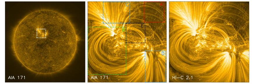
The goal of the analysis outlined here is i) from visual inspection determine a possible range of the structure observed in the Hi-C 2.1 images and ii) to measure the full width half maximum (FWHM) of these detected strands. This work samples subsections of the Hi-C 2.1 field of view (FOV), for which the data is time-averaged over a period of 60 s for both AIA and Hi-C 2.1, taking care to avoid the Hi-C 2.1 exposures impacted by the aforementioned jitter. This helps improve the signal-to-noise ratio, particularly where the emission is low. Figure 1 shows the five regions from which fourteen cross-section slices are taken. Their selection was predicated upon choosing locations where there is possible evidence of substructure or stranding within the loops, whilst taking care to avoid ares in the Hi-C 2.1 field of view where shadow of the mesh is clearly seen.
To assist in visualizing the finest structures in the Hi-C 2.1 data, we employ an image processing technique. EUV images of the corona span a wide range of features and temperatures, from cooler, low-emission coronal holes, quiet Sun, and filament channels, through to bright, hotter active regions. To account for the dominance of the bright features and reveal low-emission structures often hidden in the data, Morgan & Druckmüller (2014) developed the Multi-scale Gaussian Normalisation (MGN) technique for image processing. The method is based on localised normalisation over a range of spatial scales, and thus MGN can reveal the fine detail in the corona and structures in off-limb regions without introducing artifacts or bias. The technique is commonly used in CME and stealth CME detection (Alzate & Morgan, 2017; Hutton & Morgan, 2017; Long et al., 2018), but is also used in coronal loop studies (Chitta et al., 2017; Long et al., 2017).
Due to the way MGN enhances peaks in low-emission plasma, and depresses them in high-emission plasma, the technique is only employed in this work to improve the visual inspection of the AIA and Hi-C 2.1 data. If the FWHM calculations undertaken in §3 are done on MGN processed data, it will lead to artificially narrowed(broadened) strands in low(high)-emission plasma. Adapting the method outlined by Pant et al. (2015) in relation to the first Hi-C mission, two low-frequency passband filters are employed to both the original and MGN sharpened Hi-C 2.1 datasets to reduce the granular noise present.
In order to determine the widths of the structures, we extract the Hi-C 2.1 and AIA intensity along slices inside each sub-region; an example intensity profile is shown in the left panel of Figure 2. To further increase the signal-to-noise ratio, the slices in Hi-C 2.1 and AIA are taken to be 3 pixels wide; the intensity is then averaged over these pixels. The slices are taken perpendicular to the strand cross-section in order to obtain accurate measurements of the strand widths. The slice locations and averaged intensities in AIA and Hi-C 2.1 are given in Figures 4-8 in the first and second columns, respectively. After finding the average intensity along each slice, the global trend is removed by finding all the local minima of a slice (shown in Figure 2 as red asterisks), and interpolating through these values. The resulting trend is then subtracted from the intensity profile of the slice, leaving behind the variations, i.e. the coronal strands, seen in the right panel of Figure 2 and the third columns of Figures 4-8. The base locations of the isolated coronal strands are determined as the inflection points, and the maximum value between the two inflection points is taken as the maxima of each strand. From these two values, the half-maximum value is determined and their locations are used to determine the FWHM of each structure analysed (orange dashed lines in Figure 2). These FWHM values are used as a possible determination of the coronal strand widths, which are then compared to previous high-resolution studies.
The uncertainty in the intensity for the cross-sectional slices is determined by . If the slice under consideration is from a region where the intensity is low, will correspond to a larger proportion of the intensity than a slice from a region of greater intensity. In some instances, such as slice 10 (Figure 6), the magnitude of appears to increase once the background subtraction has occurred (variation slice 10). This is merely a consequence of the background emission being large relative to the local intensity of the coronal strands itself. Re-normalising the background subtracted slices has the effect of focusing in on the structures themselves, which thus means that will appear larger.

3 Results
In this study cross-sectional profiles are taken from structures observed within five regions, whose positions in the AIA and Hi-C 2.1 FOV are indicated in Figure 1. Table 1 indicates the average emission for all five regions investigated during the for which the data is time-averaged. As is seen in Table 1, the average emission of Region A is at least an order of magnitude lower than the other locations investigated within AR 12712. For this reason, the study is split into two parts in what we term in this paper as low-emission loops (Region A in Figure 1), and four high-emission loop regions (Regions B-E in Figure 1). The low-emission loops are shown in more detail in Figure 4, whilst the high-emission regions include a selection of loops; large loops (Figure 5), open fan loop regions (Figures 6 & 7), and some small loops close to the centre of the active region (Figure 8).
| Region in Figure 1 | Loop Type | Mean Emission Hi-C 2.1 | Mean Emission AIA |
| (DN/pixel) | (DN/pixel) | ||
| A | Low-Emission Loops | 1229.13 | 211.550 |
| B | Large Loops Bundle | 44892.5 | 3792.84 |
| C | Northern Open Fan Loops | 79550.3 | 6939.30 |
| D | Southern Open Fan Loops | 55688.6 | 4983.92 |
| E | Central Loops Bundle | 46270.3 | 3720.91 |
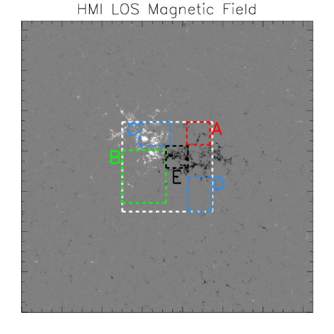
Figure 3 shows the the Helioseismic and Magnetic Imager (HMI) line-of-sight (LOS) magnetic field for the Hi-C 2.1 FOV and the surrounding area. The snapshot shown here is taken at 18:56:15 UT, which corresponds to the s period under examination with Hi-C 2.1 and AIA. From this it can be seen that AR 12712 resides above a diffuse bipolar region.
The closed magnetic loops under investigation in regions B and E very clearly have their foot-points rooted in the areas of opposite polarity, likely crossing over the active region’s polarity inversion line. The open fan loops observed in regions C and D originate from areas of opposite polarity. The low-emission strands observed in region A have one footpoint in the area of positive polarity but their negative polarity footpoint lies outside of the Hi-C 2.1 field of view. However, these low emission strands are still an integral part of the overall active region itself.
The strands in region A are low-density, and subsequently low-emission. However, due to their location and ideal viewing angle placing them away from the core of the active region, these strands can be observed in a more isolated manner, helping us to determine their widths. The coronal magnetic field is often considered to be force-free in 3D simulations (Aschwanden, 2019 and references therein), which implies that current density scales with the magnetic field (e.g. Figure 1 in Gudiksen & Nordlund, 2002). One may expect where current density is larger for the heating to be greater, and subsequently the emission to be higher. For these reasons, the study is separated into low-emission (§3.1) and high-emission (§3.2) regions.
3.1 Low-Emission Loops
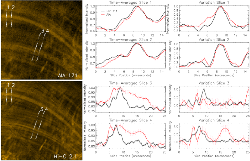
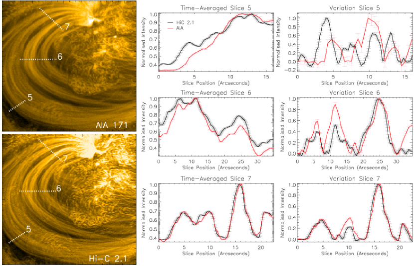
Figure 4 but for the large loops bundle in the south west quadrant of the Hi-C 2.1 FOV. Note: slice position left-to-right in the intensity plots corresponds to west-to-east orientation in the images. The error bars indicate the uncertainty in the intensity, which is defined as .
Given the way that MGN normalises a range of emission, figure 4 indicates visually the fine-scale structure that is present even in regions which may initially appear to be beneath the detection threshold. The top left panel shows the MGN sharpened AIA time-averaged data, and the bottom left panel shows the corresponding MGN sharpened Hi-C 2.1 image. From these two images, it can be seen that AIA does not have the resolution to differentiate some of the lower density, low-emission strands above the background corona and instrumental noise. Hi-C 2.1 on the other hand, performs much better with several, low-density strands being observably distinguishable.
Four data slices are taken across Region A (numbered 1-4 in Figure 4) and the normalised emission intensity along each slice is compared for Hi-C 2.1 and AIA. Each intensity profile is plotted from south to north. Slices 1 and 2 show good agreement between Hi-C 2.1 and AIA, particularly with the broader structure centred around 9′′. However, there are signs of the structure consisting of more than a single strand in Hi-C 2.1 due to the irregular shape. South of this in slice 2 there is a single strand in the AIA data () but in Hi-C 2.1 there is evidence of three coronal strands, which trace the same envelope resolved by AIA. These Hi-C 2.1 structures have FWHM between km, which is beneath the width of a single AIA pixel.
The difference between the two instruments becomes more apparent in slices 3 and 4. In the MGN sharpened images, it can be seen in the southernmost part of the slices that there are three distinct strands for Hi-C 2.1 and one to two strands in the corresponding AIA envelope. However, in the time-averaged slices for the non-MGN processed Hi-C 2.1 data, only two peaks can be seen in slice 3 (between 5′′- 12′′) and one peak in slice 4 (3′′- 11′′). This arises due to the way in which MGN normalizes and enhances over a range of spatial scales and thus cannot be employed for direct data analysis in this study.
Further north of this large envelope (), it can be seen that there is plasma detected by AIA, but this is noisy with no structure being resolved. This can be seen in the time-averaged slices as the normalised intensity value is between but no individual peaks can be identified that are above the error bars. For Hi-C 2.1 however, there are multiple strands resolved in this region, with five strands resolved between in slice 3 , and eight strands between in slice 4.
3.2 High-Emission Measure Loops
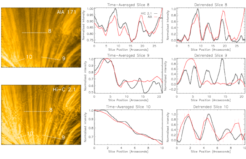
Figure 4 but for the north open fan loops in the northwest quadrant of Hi-C 2.1 FOV. Note: slice position left-to-right in the intensity plots corresponds to west-to-east orientation in the images. The error bars indicate the uncertainty in the intensity, which is defined as .
Figure 4 but for the south open fan loops in the southeast quadrant of the Hi-C 2.1 FOV. Note: slice position left-to-right in the intensity plots corresponds to west-to-east orientation in the images. The error bars indicate the uncertainty in the intensity, which is defined as .
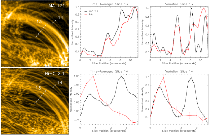
Figure 4 but for the central loops bundle between the central moss and low-emission loops. Note: slice position left-to-right in the intensity plots corresponds to south-to-north orientation in the images. The error bars indicate the uncertainty in the intensity, which is defined as .
In this subsection results from investigations of ten cross-sectional slices in the high-emission loop regions (B-E in Figure 1) are presented in the same manner as the low-emission loops discussed in §3.1. Again, the normalised intensity profiles are plotted but left-to-right orientation now corresponds to west-to-east in the respective AIA and Hi-C 2.1 images (Figures 5 - 8).
The cross-sectional slices typically show similar intensity profiles for Hi-C 2.1 and AIA, with many structures being nearly identical. In particular, slices 7 (Figure 5), 8 & 10 (Figure 6), and 11 (Figure 7) display strikingly similar overall profiles in Hi-C 2.1 and AIA. The only appreciable differences seen in slices 7 (7′′-12′′), 8 (17′′-23′′), and 10 (6′′-10′′) occur where single AIA strands correspond to two Hi-C 2.1 strands, which have widths of 562 km & 1146 km in slice 7, 1333 km & 923 km in slice 8, and 985 km & 556 km in slice 10, placing them approximately between one and three AIA pixel widths.
Similarly, there are also examples where although Hi-C 2.1 and AIA observe the same general structure, Hi-C 2.1 potentially resolves more coronal structures along the length of the cross-sections, such as is seen in slices 5 & 6 (Figure 5), and slice 13 (Figure 8). In these three slices there is reduced commonality between the two instruments as the variations are increased compared to the nearly identical cross-sections seen in slices 7, 8, 10, and 11. Focusing on slice 5, the time-averaged intensity plots of both instruments appear to show agreement; however, the corresponding detrended profile (variation plot 5 in Figure 5) reveals important differences. This can most notably be seen with the AIA structure centred at 5′′ spanning between two Hi-C 2.1 strands. Further along slice 5, the AIA structure is double peaked, with the corresponding emission coming from two distinct structures in Hi-C 2.1. Other examples can be seen in slices 6 (0′′-19′′) and 13 (1.5′′-4′′ & 7′′-13′′).
It is slices 9, 12, and 14 that the difference in resolution, and subsequently resolving power of the two instruments is most notable for the high-emission regions. Between slice position 0′′-8′′in slice 9 (Figure 6) there is a single, large structure in AIA, which can be seen as two peaks in the time-averaged Hi-C 2.1 data. This double peak is evident in the corresponding MGN Hi-C 2.1 image, whilst in the MGN AIA image the structure still appears monolithic.
Closer inspection of the two Hi-C 2.1 structures (0′′-7′′) in the variation plot reveals that the ‘monolithic’ AIA structure could actually be composed of four strands. This is because, whilst the detrended profiles of the Hi-C 2.1 structures are large, the peaks of the two structures are actually comprised of two small-peaks, which are fully-resolved and above the error bars.
The next AIA structure in slice 9 also appears as a broad, mostly unresolved single feature being detected at position 19′′. However, in the corresponding Hi-C 2.1 data there are two strands. Similarly, for the rest of the slice, Hi-C 2.1 detects two more strands; both indicating signs of possible substructure with faint double-peaks like the two aforementioned Hi-C 2.1 structures (). This highlights that there is evidence for further substructuring beyond anything that Hi-C 2.1 can observe.
In slice 12 (Figure 7) we see one of the clearest examples where the increased resolving power of Hi-C 2.1 reveals strands which AIA does not distinguish. The two large AIA features between 1′′-5′′ and 5′′-9′′each correspond to three Hi-C 2.1 strands, which have a mean width of 579 km. In Figure 8, slice 14 samples the cross-section of two strands which are relatively isolated against the underlying moss region. The southern-most strand () shows good agreement between Hi-C 2.1 and AIA in the variation plot, though again there is a non-smooth, irregular distribution in the Hi-C 2.1 data hinting at unresolved coronal strands. The northern-most strand () is well defined in Hi-C 2.1 with no obvious signs of substructure. However, in AIA there is no structure/peak at this location. The corresponding MGN sharpened AIA image reveals that the strand fades in-and-out of detection along its length, indicating this strand is at the detection threshold of AIA. This could mean that either this is a low-emission strand, or the strand has a very narrow or precise temperature which is very close to the peak emission temperature of Hi-C 2.1.
3.3 Strand Widths
A total of 25 and 49 strand widths are measured in the low-emission and high-emission regions, respectively. The appendix contains two tables that index the widths and locations of all the strands measured by Hi-C 2.1 and AIA for the low-emission (Table 2) and high-emission regions (Table 3).
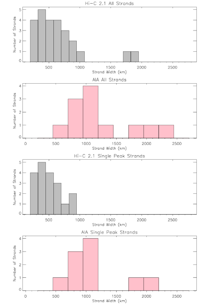
However, as can be seen in slices 3 and 12, some of the structures are double-peaked. Consequently, these result from either the presence of strands beneath the resolving power of Hi-C 2.1 or due to other coronal plasma somewhere else along the integrated line-of-sight due to the plasma being optically thin. Measuring the widths of these structures could lead to an artificially broadened distribution. Subsequently, analysis is undertaken with these double-peaked structures discarded from this survey, hence leaving 19 low-emission strands and 30 high-emission strands for width analysis. Thus, the widths are collated into occurrence frequency plots in Figure 9 for the low-emission strands and Figure 10 for the high-emission strands.
The Hi-C 2.1 occurrence frequency plot for the low-emission strand widths (Figure 9) reveals there are low-density, low-emission strands on both ends of the spatial scale, with structures as small as km, and as large as km. However, these broader structures have irregular intensity profiles (as mentioned in §3.1). Consequently, when only single-peaked structures are considered, the broader strands are between km, which is narrower than the most likely strand width measured with AIA ( km). For Hi-C 2.1, the most likely strand width of the low-emission structures is km, placing the structures at approximately the same width as an AIA pixel or smaller.
Figure 10 shows a similar distribution of strand widths for the four high-emission regions as is seen with the low-emission region. Again, narrow strands km wide are detected by Hi-C 2.1 though these are not as prevalent as in the low-emission region despite a larger sample of structures being investigated. Additionally, broader strands with widths km are observed in the high-emission regions, with one strand in slice 11 () exceeding a width of 2000 km. The most likely strand width for single-peaked structures in the four high-emission regions is between km. Considering the smallest partially resolved structure by AIA ( km) is larger than the average low-emission strand width resolved by Hi-C 2.1 ( km), it could be argued that these results, alongside those from the maiden flight of Hi-C, provide compelling evidence for satellite-borne instrumentation with the resolving power of at least Hi-C.
For AIA, the most likely strand width of the low-emission and high-emission regions are the same ( km) but for Hi-C 2.1 the low-emission strands are approximately 125 km narrower than those resolved in the high-emission region ( km vs km). It is worth noting that there is a greater proportion of the low-emission strands with widths between km compared to the high-emission strands. Conversely, the high-emission strands often exhibit widths km, agreeing with results from Peter et al. (2013), whilst the low-emission strand widths do not exceed km in this study.
4 Concluding Remarks
Continuing on from the success of Hi-C, Hi-C 2.1 reveals structures throughout and around its targeted active region (AR 12712) in the 17.2 nm line that cannot be resolved by SDO/AIA. The work outlined here investigates five regions from the Hi-C 2.1 FOV, one region of what could be considered low-emission and four regions of significantly increased emission (Figure 1).
In regard to Region A, although it could be argued that there are hints of faint structures that could be observed in the AIA FOV, it is found that with Hi-C 2.1’s superior resolving power, this region is in fact filled with numerous low emitting, and hence low-density strands. In AIA, these strands often appear as granular noise. A contributing factor to this is that these low-emission strands are observed by Hi-C 2.1 to be of only km in width, beneath the scale of a single AIA pixel.
In contrast, Regions B-E have higher emission structures with an average Hi-C 2.1 strand width of km, placing them in line with previous width measurements made using Hi-C (Brooks et al., 2013; Aschwanden & Peter, 2017). As discussed in Peter et al. (2013) with regards to miniature loops, the Hi-C 2.1 data reveals strand widths as small as 200 km in both the low-emission and high-emission regions, though they appear to be more numerous in the low-emission area of the active region.
An intriguing result is outlined in the analysis of slice 14, which samples the cross-section of the closed active region loops near the centre of the Hi-C 2.1 FOV. In the MGN sharpened AIA image (Figure 8), the northern-most strand sampled in slice 14 appears to fade in-and-out of AIA detection along its length. This suggests that the plasma contained within this structure is at the sensitivity limit of AIA, even when advanced image processing techniques like MGN are employed. Either this is a low-emission strand amongst the high-emission structures, or this may simply be due to the fact that AIA and Hi-C 2.1 observe plasma at slightly different temperatures (17.1nm and 17.2nm emission).
The evidence for low-emission strands, which are very difficult to observe with AIA but much better resolved and width determined by Hi-C 2.1, strongly indicates that plasma threads with low-density but coronal temperature material are prevalent throughout the corona. This may be a strong indicator of previously unresolved, but background heated corona that Hi-C 2.1 is beginning to provide evidence for. However, even with the enhanced spatial resolution of Hi-C 2.1, it still appears that there are structures which could not be fully resolved. Although this could be due to projection effects of the optically thin plasma viewed along its line-of-sight, another possible scenario is that there are coronal strands with structural widths below even the resolving power of Hi-C 2.1.
Slices 9 & 12 are good examples of this but there are hints of substructure above the observational error throughout all the slices examined. Thus, it may be possible for an instrument of greater resolving power to discriminate between these features. Note that by combining both FFT and Gaussian width analysis methods, Rachmeler et al. (2019) conclude that the Hi-C 2.1 resolution is between ( km) in images that are not affected by motion blur. The most-likely strand widths obtained for the low-emission strands ( km) are above the resolution limit of Hi-C 2.1, indicating that at this increased spatial resolution we may be beginning to have the opportunity resolve a fundamental width of individual coronal strands. This result agrees with the results from Aschwanden & Peter (2017) though we note that there is building evidence that there are strands with widths beneath the Hi-C 2.1 resolution.
Additionally, it may be argued that spatial structuring is only one part of the data required to address this question of basic plasma stranding as the spread of observed temperature of these features is also critical. If the 17.2 nm Hi-C 2.1 structures that are observed to be beneath the AIA resolution limit could also be observed in other passbands with similar spatial resolution to Hi-C 2.1 and those observations then resulted in a broad temperature distribution of many strand-like features, then this could be strong evidence for multi-thermal, many stranded models being the best way tackle coronal heating.
Future work will further examine the double-peaked structures by fitting appropriate Gaussian profiles in order to estimate the widths of the possible sub-resolution strands, as well as consider the examination of the extrapolated magnetic field structure associated with low-emission strands alongside a comparison of the Hi-C 2.1 observations with specific active region modelling (Warnecke & Peter, 2019).
References
- Alexander et al. (2013) Alexander, C. E., Walsh, R. W., Régnier, S., Cirtain, J. W., Winebarger, A. R., Golub, L., Kobayashi, K., Platt, S., Mitchell, N., Korreck, K., De Pontieu, B., DeForest, C., Weber, M.,Title, A., Kuzin, S. 2013, ApJ, 775, L32
- Alzate & Morgan (2017) Alzate, N., Morgan, H. 2017, ApJ, 840, 103
- Antiochos et al. (2003) Antiochos, S. K., Karpen, J. T., DeLuca, E. E., Golub, L., Hamilton, P. 2003, ApJ, 590, 547
- Aschwanden (2004) Aschwanden, M. J. 2004, Physics of the Solar Corona: An Introduction (New York: Springer)
- Aschwanden (2019) Aschwanden, M. J. 2019, ApJ, 885, 49
- Aschwanden & Nightingale (2005) Aschwanden, M. J., Nightingale, R. W. 2005, ApJ, 633, 499
- Aschwanden & Peter (2017) Aschwanden M. J., Peter, H. 2017 ApJ, 840, 4
- Barczynski et al. (2017) Barczynski, K., Peter, H., Savage, S. L. 2017, A&A, 599, A137
- Berger et al. (1999) Berger, T. E., De Pontieu, B., Fletcher, L., Schrijver, C. J., Tarbell, T. D., Title, A. M. 1999, Sol. Phys., 190, 409
- Bray et al. (1991) Bray, R. J., Cram, L. E., Durrant, C., Loughhead, R. E. 1991, Plasma Loops in the Solar Corona (Cambridge: Cambridge University Press)
- Bradshaw & Cargill (2013) Bradshaw, S. J., Cargill, P. J. 2013, ApJ, 770, 12
- Brooks et al. (2013) Brooks, D. H., Warren, H. P., Ugarte-Urra, I., Winebarger, A. R. 2013, ApJ, 772, L19
- Brooks et al. (2016) Brooks, D. H., Reep, J. W., Warren, H. P. 2016, ApJ, 826, L18
- Cargill & Klimchuk (2004) Cargill, P. J., Klimchuk, J. A. 2004, ApJ, 605, 911
- Chitta et al. (2017) Chitta, L. P., Peter, H., Solanki, S. K., Barthol, P., Gandorfer, A., Gizon, L., Hirzberger, J., Riethmüller, van Noort, M., Blanco Rodríguez, 2017, ApJS, 229, 4
- Cirtain et al. (2007) Cirtain, J. W., Del Zanna, G., DeLuca, E. E., Mason, H. E., Martens, P. C. H., Schmelz, J. T., ApJ, 655, 598
- Cirtain et al. (2013) Cirtain, J. W., Golub, L., Winebarger, A. R., de Pontieu, B., Kobayashi, K., Moore, R. L., Walsh, R. W., Korreck, K. E., Weber, M., McCauley, P., Title, A., Kuzin, S., Deforest, C. E. 2013, Nature, 493, 501
- Delaboudinière et al. (1995) Delaboudinière, J. P., Artzner, G. E., Brunaud, J., Gabriel, A. H., Hochedez, J. F., Millier, F., Song, X. Y., Au, B., Dere, K. P., Howard, R. A., Kreplin, R., Michels, D. J., Moses, J. D., Defise, J. M., Jamar, C., Rochus, P., Chauvineau, J. P., Marioge, J. P., Catura, R. C., Lemen, J. R., Shing, L., Stern, R. A., Gurman, J. B., Neupert, W. M., Maucherat, A., Clette, F., Cugnon, P., Van Dessel, E. L. 1995, Sol. Phys., 162, 291
- De Pontieu et al. (2014) De Pontieu, B., Title, A. M., Lemen, J. R., Kushner, G. D., Akin, D. J., Allard, B., Berger, T., Boerner, P., Cheung, M., Chou, C., Drake, J. F., Duncan, D. W., Freeland, S., Heyman, G. F., Hoffman, C., Hurlburt, N. E., Lindgren, R. W., Mathur, D., Rehse, R., Sabolish, D. Seguin, R., Schrijver, C. J., Tarbell, T. D., Wülser, J.-P., Wolfson, C. J., Yanari, C., Mudge, J., Nguyen-Phuc, N., Timmons, R., van Bezooijen, R., Weingrod, I., Brookner, R., Butcher, G., Dougherty, B., Eder, J., Knagenhjelm, V., Larsen, S., Mansir, D., Phan, L., Boyle, P., Cheimets, P. N., DeLuca, E. E., Golub, L., Gates, R., Hertz, E., McKillop, S., Park, S., Perry, T., Podgorski, W. A., Reeves, K., Saar, S., Testa, P., Tian, H., Weber, M., Dunn, C., Eccles, S., Jaeggli, S. A., Kankelborg, C. C., Mashburn, K., Pust, N., Springer, L., Carvalho, R., Kleint, L., Marmie, J., Mazmanian, E., Pereira, T. M. D., Sawyer, S.,Strong, J., Worden, S. P., Carlsson, M., Hansteen, V. H., Leenaarts, J., Wiesmann, M.; Aloise, J., Chu, K.-C., Bush, R. I., Scherrer, P. H., Brekke, P., Martinez-Sykora, J., Lites, B. W., McIntosh, S. W., Uitenbroek, H., Okamoto, T. J., Gummin, M. A., Auker, G., Jerram, P., Pool, P., Waltham, N. 2014, Sol. Phys., 289, 2733
- Feldman (1983) Feldman, U. 1983, ApJ, 275, 367
- Gudiksen & Nordlund (2002) Gudiksen, B., Nordlund, A. 2002, ApJ, 572, L113
- Handy et al. (1999) Handy, B. N., Acton, L. W., Kankelborg, C. C., Wolfson, C. J., Akin, D. J., Bruner, M. E., Caravalho, R., Catura, R. C., Chevalier, R., Duncan, D. W., Edwards, C. G., Feinstein, C. N., Freeland, S. L., Friedlaender, F. M., Hoffmann, C. H., Hurlburt, N. E., Jurcevich, B. K., Katz, N. L., Kelly, G. A., Lemen, J. R., Levay, M., Lindgren, R. W., Mathur, D. P., Meyer, S. B., Morrison, S. J., Morrison, M. D., Nightingale, R. W., Pope, T. P., Rehse, R. A., Schrijver, C. J., Shine, R. A., Shing, L., Strong, K. T., Tarbell, T. D., Title, A. M., Torgerson, D. D., Golub, L., Bookbinder, J. A., Caldwell, D., Cheimets, P. N., Davis, W. N., Deluca, E. E., McMullen, R. A., Warren, H. P., Amato, D., Fisher, R., Maldonado, H., Parkinson, C. 1999, Sol. Phys., 187, 229
- Hutton & Morgan (2017) Hutton, J., Morgan, H. 2017, A&A, 599, A68
- Kobayashi et al. (2014) Kobayashi, K., Cirtain, J., Winebarger, A. R., Korreck K., Golub, L., Walsh, R. W., De Pontieu, B., DeForest, C., Title, A. M., Kuzin, S., Savage, S., Beabout, D., Beabout, B., Podgorski, W. 2014, Sol. Phys., 289, 4393
- Lemen et al. (2012) Lemen, J. R., Title, A. M., Akin, D. J., Boerner, P. F., Chou, C., Drake, J. F., Duncan, D. W., Edwards, C. G., Friedlaender, F. M., Heyman, G. F., Hurlburt, N. E., Katz, N. L., Kushner, G. D., Levay, M., Lindgren, R. W. 2012, Sol. Phys., 275, 17
- Long et al. (2017) Long, D. M., Valori, G., Pérez-Suaréz, D., Morton, R. J., Vásquez A. M. 2017, A&A, 603, A101
- Long et al. (2018) Long D. M., Harra, L. K., Matthews, S. A., Warren, H. P., Lee, K-S., Doschek, G. A., Hara, H., Jenkins, J. 2018, ApJ, 855, 74
- Morgan & Druckmüller (2014) Morgan, H., Druckmüller, M. 2014, Sol. Phys., 289, 2945
- Mulu-Moore et al. (2011) Mulu-Moore F. M., Winebarger A. R., Warren H. P., Aschwanden M. J. 2011 ApJ, 733, 59
- Pant et al. (2015) Pant, V., Datta, A., Banerjee, D. 2015, ApJ, 801, L2
- Peter et al. (2013) Peter, H., Bingert, S., Klimchuk, J. A., de Forest, C., Cirtain, J. W., Golub, L., Winebarger, A. R., Kobayashi, K., Korreck, K. E. 2013, A&A, 556, A104
- Pontin et al. (2017) Pontin, D. I., Janvier, M., Tiwari, S. K., Galsgaard, K., Winebarger, A. R., Cirtain, J. W. 2017, ApJ, 837, 108
- Price & Taroyan (2015) Price, D. J.,Taroyan, Y. 2015, Annales Geophysicae, 33, 25
- Rachmeler et al. (2019) Rachmeler, A. L., Winebarger, A. R., Savage, A. L., Golub, L., Kobayashi, K., Vigil, G. D., Brooks, D. H., Cirtain, J. W., De Pontieu, B., McKenzie, D. E., Morton, R. J., Peter, H., Testa, P., Tiwari, S. K., Walsh, R. W., Warren, H. P., Alexander, C., Ansell, D., Beabout, B. L., Beabout, D. L., Bethge, C. W., Champey, P. R., Cheimets, P. N., Cooper, M. A., Creel, H. K., Gates, R., Gomez, C., Guillory, A., Haight, H., Hogue, W. D., Holloway, T., Hyde, D. W., Kenyon, R., Marshall, J. N., McCracken, J. E., McCracken, K., Mitchell, K. O., Ordway, M., Owen, T., Ranganathan, J., Robertson, B. A., Payne, M. J., Podgorski, W., Pryor, J., Samra, J., Sloan, M. D., SooHoo, H. A., Steele, D. B., Thompson, F. V., Thornton, G. S., Watkinson, B., Windt, D. 2019, Sol. Phys., in prep
- Reale (2010) Reale, F. 2010, Living Reviews in Solar Physics, 7, 5
- Sarkar & Walsh (2008) Sarkar, A., & Walsh, R. W. 2008, ApJ, 683, 516
- Sarkar & Walsh (2009) Sarkar, A., & Walsh, R. W. 2009, ApJ, 699, 1480
- Schmelz et al. (2001) Schmelz T. J., Scopes, R. T., Cirtain, J. W., Winter, H. D., Allen, J. D. 2001, ApJ, 556, 896
- Schmelz (2002) Schmelz T. J. 2002, ApJ, 578, L161
- Schmelz et al. (2009) Schmelz, T. J., Nasraoui, K., Rightmire, L. A., Kimble, J. A., Del Zanna, G., Cirtain, J. W., DeLuca, E. E., Mason H. E. 2009, ApJ, 691, 503
- Taroyan et al. (2011) Taroyan, Y., Erdélyi, R., Bradshaw, S. J. 2011, Sol. Phys., 269, 295
- Testa et al. (2013) Testa, P., De Pontieu, B., Martínez-Sykora, J., De Luca, E., Hansteen, V., Cirtain, J. W., Winebarger, A. R., Golub, L., Kobayashi, K., Korreck, K., Kuzin, S., Walsh, R. W., DeForest, C., Title, A., Weber, M. 2013, ApJ, 770, 1
- Thalmann et al. (2014) Thalmann, J. K., Tiwari, S. k., Wiegelmann, T. 2014, ApJ, 780, 102
- Tiwari et al. (2014) Tiwari, S. K., Alexander, C. E., Winebarger, A. R., Moore, R. L. 2014, ApJ, 795, L24
- Tripathi et al. (2009) Tripathi D., Mason H. E., Dwivedi B. N., del Zanna G., Young P. R. 2009 ApJ, 694, 1256
- Warnecke & Peter (2019) Warnecke, J., Peter, H. 2019, A&A, 624, L12
- Warren et al. (2002) Warren, H., Winebarger A. R., Hamilton, P. S. 2002, ApJ, 679, L41
- Warren et al. (2010) Warren, H. P., Winebarger, A. R., Brooks, D. H. 2010, ApJ, 711, 228
- Warren et al. (2011) Warren, H. P., Brooks, D. H., Winebarger, A. R. 2011, ApJ, 734, 90
- Winebarger et al. (2002) Winebarger, A. R., Warren, H. P., van Ballegooijen, A., DeLuca, E. E., Golub, L. 2002, ApJ, 567, L89
- Winebarger et al. (2003) Winebarger, A. R., Warren, H. P., Seaton, D. B. 2003, ApJ, 593, 1164
- Winebarger et al. (2013) Winebarger, A. R., Walsh, R. W., De Pontieu, B., Hansteen, V., Cirtain, J. W., Golub, L., Kobayashi, K., Korreck, K., DeForest, C., Title, A., Kuzin, S. 2013, ApJ, 771, 21
In this appendix we present Tables 2 & 3. These show all the strands where FWHM calculations were possible. The widths shown in bold with an asterisks denote strands which display obvious signs of sub-resolution and/or overlapping strands, and are thus omitted from final statistical analysis on the widths.
| Hi-C 2.1 | AIA 171Å | ||||||
| Slice # | Start Position (′′) | End Position (′′) | FWHM (km) | Slice # | Start Position (′′) | End Position (′′) | FWHM (km) |
| 1 | 0.000 | 1.968 | 697.5 | ||||
| 1 | 1.968 | 3.150 | 473.6 | ||||
| 1 | 4.987 | 5.906 | 381.2 | 1 | 4.200 | 13.20 | 2383.8* |
| 1 | 5.906 | 11.28 | 1819.4* | ||||
| 1 | 12.20 | 13.51 | 409.8 | ||||
| 2 | 0.000 | 1.050 | 226.6 | ||||
| 2 | 1.050 | 2.625 | 345.2 | 2 | 1.800 | 6.600 | 1373.4* |
| 2 | 2.625 | 3.937 | 359.4 | ||||
| 2 | 4.200 | 5.643 | 395.5 | 2 | 6.600 | 12.60 | 2041.6 |
| 2 | 6.037 | 11.81 | 1859.0* | ||||
| 3 | 1.806 | 4.644 | 733.9 | 3 | 0.600 | 4.200 | 838.7 |
| 3 | 5.031 | 7.224 | 822.0* | 3 | 5.400 | 7.800 | 853.2 |
| 3 | 7.224 | 10.57 | 928.9 | 3 | 7.800 | 10.80 | 1062.1 |
| 3 | 14.06 | 15.73 | 552.0 | 3 | 15.00 | 17.40 | 642.6 |
| 3 | 16.12 | 18.31 | 590.9 | 3 | 17.40 | 21.00 | 1130.1 |
| 3 | 18.83 | 21.02 | 972.0* | 3 | 21.00 | 23.40 | 925.7 |
| 3 | 21.02 | 22.96 | 620.5* | ||||
| 4 | 11.61 | 12.25 | 215.7 | 4 | 4.200 | 6.600 | 951.2 |
| 4 | 12.65 | 13.67 | 664.6 | ||||
| 4 | 14.06 | 14.96 | 318.0 | 4 | 6.600 | 10.80 | 1829.0 |
| 4 | 14.96 | 16.12 | 527.4 | ||||
| 4 | 16.12 | 16.89 | 216.8 | 4 | 13.20 | 21.00 | 2701.2 |
| 4 | 17.93 | 19.35 | 466.7 | ||||
| 4 | 19.73 | 21.67 | 863.7 | 4 | 21.60 | 24.60 | 959.9 |
| 4 | 21.67 | 23.09 | 717.4* | ||||
| Hi-C 2.1 | AIA 171Å | ||||||
| Slice # | Start Position (′′) | End Position (′′) | FWHM (km) | Slice # | Start Position (′′) | End Position (′′) | FWHM (km) |
| 5 | 0.000 | 1.712 | 528.5 | ||||
| 5 | 1.913 | 5.640 | 1346.6* | 5 | 3.748 | 6.559 | 1547.6 |
| 5 | 9.267 | 11.88 | 1190.5* | 5 | 8.901 | 12.18 | 1513.0 |
| 5 | 11.88 | 14.20 | 871.2 | 5 | 12.18 | 14.52 | 1137.4 |
| 5 | 14.40 | 15.31 | 202.2 | ||||
| 6 | 4.515 | 8.256 | 1046.0 | 6 | 0.600 | 2.400 | 895.2 |
| 6 | 8.256 | 9.417 | 355.8 | 6 | 2.400 | 7.800 | 1781.3* |
| 6 | 9.417 | 13.15 | 1047.7 | 6 | 7.800 | 16.20 | 2840.0 |
| 6 | 30.18 | 32.89 | 1107.1 | 6 | 16.20 | 18.60 | 893.8 |
| 7 | 1.783 | 7.220 | 2304.5* | 7 | 1.975 | 7.506 | 2279.2* |
| 7 | 7.220 | 8.749 | 562.0 | 7 | 7.506 | 13.03 | 1577.4 |
| 7 | 8.749 | 11.38 | 1146.1 | 7 | 13.03 | 19.75 | 1722.2* |
| 7 | 13.25 | 19.19 | 1862.4* | 7 | 19.75 | 22.91 | 1135.9 |
| 7 | 19.53 | 22.42 | 1028.8 | ||||
| 8 | 1.806 | 4.386 | 810.6 | 8 | 1.200 | 4.800 | 819.5 |
| 8 | 4.386 | 10.96 | 2453.3* | 8 | 4.800 | 10.20 | 2550.0* |
| 8 | 10.96 | 15.35 | 1775.4 | 8 | 10.20 | 15.60 | 1571.2* |
| 8 | 16.51 | 20.51 | 1333.7 | 8 | 16.80 | 22.80 | 1782.1 |
| 8 | 20.51 | 22.70 | 922.7* | 8 | 22.80 | 24.60 | 708.2 |
| 8 | 24.76 | 27.47 | 676.9 | ||||
| 9 | 0.000 | 4.164 | 1509.6* | ||||
| 9 | 4.164 | 7.192 | 1180.6* | 9 | 0.000 | 7.630 | 3241.7 |
| 9 | 7.823 | 11.60 | 1392.5* | 9 | 7.630 | 10.56 | 1083.7 |
| 9 | 11.60 | 15.52 | 1145.8* | 9 | 11.73 | 13.49 | 736.6 |
| 9 | 17.41 | 19.18 | 646.0* | 9 | 15.26 | 17.02 | 536.6 |
| 9 | 19.18 | 21.07 | 750.7 | 9 | 17.02 | 21.71 | 1374.2 |
| 10 | 0.369 | 3.447 | 1071.2* | 10 | 0.000 | 3.436 | 1306.2 |
| 10 | 3.447 | 6.156 | 975.4 | 10 | 3.436 | 6.299 | 1143.2 |
| 10 | 6.156 | 8.618 | 984.9 | 10 | 6.299 | 9.735 | 969.1* |
| 10 | 8.618 | 10.09 | 556.3 | ||||
| 11 | 0.258 | 4.515 | 1622.4 | 11 | 0.000 | 4.800 | 1939.5 |
| 11 | 4.515 | 9.417 | 1718.9* | 11 | 4.800 | 10.20 | 1504.7 |
| 11 | 18.96 | 24.63 | 2069.9 | 11 | 18.60 | 27.00 | 3116.1 |
| 12 | 0.121 | 1.274 | 387.2 | ||||
| 12 | 1.274 | 3.096 | 830.9* | 12 | 0.000 | 1.129 | 532.8 |
| 12 | 3.096 | 4.128 | 346.4 | ||||
| 12 | 4.128 | 5.524 | 571.9 | 12 | 1.129 | 5.364 | 1485.1* |
| 12 | 5.524 | 6.799 | 451.6 | ||||
| 12 | 6.799 | 8.316 | 534.0 | 12 | 5.364 | 9.317 | 1633.6* |
| 12 | 8.316 | 9.834 | 738.7* | ||||
| 13 | 0.081 | 2.042 | 560.5* | 13 | 0.000 | 1.159 | 589.8 |
| 13 | 2.042 | 3.185 | 382.2 | ||||
| 13 | 3.349 | 4.084 | 263.3 | 13 | 4.179 | 6.838 | 977.6 |
| 13 | 4.084 | 6.371 | 795.4* | ||||
| 13 | 7.270 | 9.149 | 582.1 | 13 | 7.598 | 9.498 | 466.6 |
| 13 | 9.149 | 10.04 | 400.0 | ||||
| 13 | 10.04 | 11.51 | 574.9 | 13 | 9.498 | 11.77 | 967.4 |
| 14 | 0.000 | 1.733 | 685.2* | 14 | 0.000 | 2.121 | 571.6 |
| 14 | 1.915 | 3.739 | 478.4 | ||||