Towards Power-Efficient Aerial Communications via Dynamic Multi-UAV Cooperation

Abstract

Aerial base stations (BSs) attached to unmanned aerial vehicles (UAVs) constitute a new paradigm for next-generation cellular communications. However, the flight range and communication capacity of aerial BSs are usually limited due to the UAVs’ size, weight, and power (SWAP) constraints. To address this challenge, in this paper, we consider dynamic cooperative transmission among multiple aerial BSs for power-efficient aerial communications. Thereby, a central controller intelligently selects the aerial BSs navigating in the air for cooperation. Consequently, the large virtual array of moving antennas formed by the cooperating aerial BSs can be exploited for low-power information transmission and navigation, taking into account the channel conditions, energy availability, and user demands. Considering both the fronthauling and the data transmission links, we jointly optimize the trajectories, cooperation decisions, and transmit beamformers of the aerial BSs for minimization of the weighted sum of the power consumptions required by all BSs. Since obtaining the global optimal solution of the formulated problem is difficult, we propose a low-complexity iterative algorithm that can efficiently find a Karush-Kuhn-Tucker (KKT) solution to the problem. Simulation results show that, compared with several baseline schemes, dynamic multi-UAV cooperation can significantly reduce the communication and navigation powers of the UAVs to overcome the SWAP limitations, while requiring only a small increase of the transmit power over the fronthauling links.

I Introduction

Exploiting unmanned aerial vehicles (UAVs) or drones as aerial base stations (BSs) for enhanced cellular communication has recently attracted significant interest [1, 2]. Unlike terrestrial BSs whose communication with ground users is usually subject to non-line-of-sight (NLoS) channels, aerial BSs can proactively seek line-of-sight (LoS) connections with ground users to facilitate favorable signal propagation. Moreover, the deployment of UAVs can be adapted on demand to the spatial and temporal distributions of the cellular users under both normal and contingency conditions. Yet, aerial BSs are usually constrained in size, weight, and power supply (SWAP) and have only limited flight range and communication capabilities [3]. Therefore, improving the navigation and communication performance of aerial BSs within the SWAP limits is a crucial research challenge.

A promising approach is to employ an array of networked UAVs, whereby the existing aerial communication schemes for networked UAVs can be classified into non-cooperative [4, 5] and cooperative [6, 7] schemes. For the non-cooperative schemes, the navigation/communication tasks are divided among the UAVs across time and space, which leads to low payload and low communication overheads per UAV [4]. However, these schemes require orthogonal spectrum allocation for the UAVs and coexisting terrestrial BSs/users, leading to a low spectrum utilization. Otherwise, LoS co-channel interferers may severely degrade the reliability of aerial communications [8, 9].

To boost network capacity, multi-UAV cooperation with full frequency reuse, akin to the multi-cell cooperation paradigm in cellular communications [10], has been proposed. In [6], multiple UAVs hovering in the air are utilized as aerial remote radio heads (RRHs) to communicate with ground users in the uplink, and the signals received at each UAV are forwarded to a central processor for joint decoding. The authors investigate the optimal placement and movement of the UAVs for maximization of the minimal achievable rate of the users [6]. A BS cooperation scheme for canceling the interference caused by multi-antenna UAVs is proposed in [7]. In particular, each BS forwards its decoded message(s) to the other BSs via backhaul links, which are then exploited for interference cancellation. The authors in [7] investigate optimal beamforming for maximization of the sum rate for UAVs hovering at fixed positions.

The aforementioned works [4, 5, 6, 7] assume the non-cooperation and cooperation among UAVs to be fixed over time and space. However, due to the UAVs’ mobility and the heterogeneity of the terrain features, the signal and interference powers in aerial networks may vary significantly along the UAVs’ flying trajectories, which cannot be properly exploited with the existing static schemes. To further unlock the potential of networked UAVs, in this paper, we introduce the new concept of dynamic multi-UAV cooperation. Thereby, the UAVs are intelligently selected for cooperation with other UAVs, taking into account their positions/trajectories, channel and energy conditions, and the users’ demands. By exploiting the resulting large virtual array of moving antennas for cooperative data transmission, the UAVs’ mechanical navigation and cooperative beamforming provide additional spatial degrees of freedom for facilitating power-efficient aerial communications.

To maximize the benefits of dynamic multi-UAV cooperation within the SWAP constraints, we jointly optimize the UAVs’ trajectories, cooperation decisions, and cooperative beamformers for minimization of the weighted sum of the BSs’ power consumptions while guaranteeing the quality of service (QoS) of the users and safe navigation of the UAVs. The formulated problem is a mixed-integer non-convex program and finding the global optimal solution is generally NP-hard. To tackle this issue, we exploit the underlying difference of convex (DC) program structure and propose a low-complexity suboptimal scheme based on binary approximation and the convex-concave procedure (CCP) [11]. Under mild conditions, the solution to the joint optimization problem found by the proposed algorithm fulfills the Karush–Kuhn–Tucker (KKT) optimality conditions of the original non-convex problem. The contributions of this paper are summarized as follows:

• We propose dynamic multi-UAV cooperation, where each UAV can intelligently cooperate with other UAVs during navigation, to enable power-efficient aerial communication.

• We develop a low-complexity algorithm for joint optimization of the UAVs’ cooperation, the fronthauling and data transmission, and the UAVs’ trajectories to minimize the weighted sum of the BSs’ power consumptions required for communication and navigation.

• Our simulation results show that dynamic multi-UAV cooperation can significantly improve the power efficiency of UAV communication and navigation despite the UAVs’ SWAP constraints.

Notations: Throughout this paper, $\mathbb{R}$, $\mathbb{R}_{+}$, and $\mathbb{C}$ denote the sets of real, non-negative real, and complex numbers, respectively. $\mathbb{C}^{N}$ and $\mathbb{C}^{N\times M}$ are the sets of complex $N\times 1$ vectors and $N\times M$ matrices, respectively. $\mathbf{I}_{N}$ is the $N\times N$ identity matrix. $\Re\left\{\mathbf{z}\right\}$ and $\Im\left\{\mathbf{z}\right\}$ denote the real and imaginary parts of complex-valued vector $\mathbf{z}\in\mathbb{C}^{N}$, respectively. $(\cdot)^{\mathrm{T}}$, $(\cdot)^{\mathrm{H}}$, $\mathrm{tr}(\cdot)$, and $\mathrm{rank}(\cdot)$ are the transpose, complex conjugate transpose, trace, and rank operators, respectively. $\left|\cdot\right|$, $\left\|\cdot\right\|$, and $\left\|\cdot\right\|_{F}$ denote the absolute value of a scalar, the $\ell_{2}$-norm of a vector, and the Frobenius-norm of a matrix, respectively. $\mathbf{x}\preceq\mathbf{y}$ ($\mathbf{x}\succeq\mathbf{y}$) means that vector $\mathbf{x}$ is element-wise smaller (greater) than or equal to vector $\mathbf{y}$. $\mathcal{CN}\left(\mu,\sigma^{2}\right)$ represents the complex Gaussian distribution with mean $\mu$ and variance $\sigma^{2}$. Finally, $\nabla f(\mathbf{x})$ is the gradient of function $f(\mathbf{x})$ with respect to $\mathbf{x}$.

II System Model

We assume that $L$ UAVs, each mounted with a cellular transceiver (aerial BS), are deployed for providing downlink communications to $K$ ground users, see Figure 1. Let $\mathcal{L}\triangleq\left\{1,\ldots,L\right\}$ and $\mathcal{K}\triangleq\left\{1,\ldots,K\right\}$ denote the index sets of the UAVs and the users, respectively. The UAVs employ wireless fronthauling by connecting to a remote ground BS. The ground BS and each UAV are equipped with $N\geq 1$ and $M\geq 1$ antennas, respectively, whereas the users are single-antenna devices. We assume $N\geq L$ and $LM\geq K$ to ensure a feasible problem formulation. Moreover, due to large propagation distances and potential blockages, the users of interest cannot establish a direct connection to the ground BS. Therefore, information transmission to these users comprises (i) fronthauling from the ground BS to the UAVs and (ii) data transmission from the UAVs to the users. We consider a time-slotted system. Each time slot is divided into two intervals of equal duration, where fronthauling and data transmission are performed the first and the second interval of each time slot, respectively.

The UAVs may navigate within a given aerial space to facilitate communication with the ground BS and the users. However, depending on the UAVs’ positions, the channel conditions for aerial communications, including the LoS/NLoS propagation paths and the interference caused by multi-UAV fronthauling and data transmission, may vary significantly. Hence, dynamic cooperation among the UAVs is desirable to coordinate information transmission, interference mitigation, and navigation in real-time. In the following, we first investigate the underlying aerial-to-ground channels and then present the aerial communication design tailored to the channel characteristics.

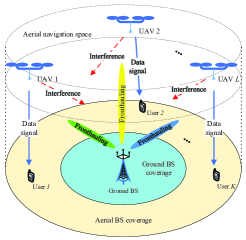
Figure 1: Illustration of multi-UAV assisted downlink communication for users whose connections to the ground BS are blocked.

II-A Channel Modeling

Let $\mathbf{d}_{k}^{\mathrm{UE}}\triangleq\left[d_{k,x}^{\mathrm{UE}},d_{k,y}^{\mathrm{UE}},d_{k,z}^{\mathrm{UE}}\right]^{\mathrm{T}}\in\mathbb{R}^{3}$ and $\mathbf{d}^{\mathrm{BS}}\triangleq\left[d_{x}^{\mathrm{BS}},d_{y}^{\mathrm{BS}},d_{z}^{\mathrm{BS}}\right]\in\mathbb{R}^{3}$ denote the fixed positions of user $k\in\mathcal{K}$ and the ground BS, respectively. Furthermore, $\mathbf{d}_{l,t}\triangleq\left[d_{l,x,t},d_{l,y,t},d_{l,z,t}\right]^{\mathrm{T}}\in\mathbb{R}^{3}$ denotes the position of UAV $l\in\mathcal{L}$ at time $t$. The distance between UAV $l$ and user $k$ at time $t$ is thus given by

$$d_{l,k,t}\triangleq\left\|\mathbf{d}_{l,t}-\mathbf{d}_{k}^{\mathrm{UE}}\right\|$$

$$=\sqrt{(d_{l,x,t}-d_{k,x}^{\mathrm{UE}})^{2}\!+\!(d_{l,y,t}-d_{k,y}^{\mathrm{UE}})^{2}\!+\!(d_{l,z,t}-d_{k,z}^{\mathrm{UE}})^{2}}.$$

Likewise, the distance between UAV $l$ and the ground BS at time $t$ is $d_{\mathrm{F},l,t}\triangleq\left\|\mathbf{d}_{l,t}-\mathbf{d}^{\mathrm{BS}}\right\|$. Due to ground reflections and scattering, data signals transmitted over the UAV-to-user channel may undergo both LoS and NLoS propagation. Let $\mathbf{h}_{l,k,t}\in\mathbb{C}^{M\times 1}$ be the channel gain vector between UAV $l$ and user $k$ at time $t$. We assume $\mathbf{h}_{l,k,t}=\sqrt{A_{l,k}d_{l,k,t}^{-\alpha_{l,k}}}\mathbf{g}_{l,k,t}$, where $A_{l,k}d_{l,k,t}^{-\alpha_{l,k}}$ and $\mathbf{g}_{l,k,t}\in\mathbb{C}^{M}$ capture the propagation path loss and the channel gains due to multipath fading, respectively. $\alpha_{l,k}$ is the path loss exponent of the channel between UAV $l$ and user $k$, and $A_{l,k}$ is a constant accounting for the antenna gains.

On the other hand, as both antenna arrays are elevated, the ground BS-to-UAV fronthauling channels are usually dominated by LoS propagation. Let $\mathbf{H}_{\mathrm{F},l,t}\in\mathbb{C}^{N\times M}$ be the channel matrix between the ground BS and UAV $l$ at time $t$. Without loss of generality, we assume $\mathbf{H}_{\mathrm{F},l,t}=\sqrt{A_{\mathrm{F},l}d_{\mathrm{F},l,t}^{-\alpha_{\mathrm{F},l}}}\mathbf{G}_{\mathrm{F},l,t}$, where $\alpha_{\mathrm{F},l}$ and $A_{\mathrm{F},l}$ denote the path loss exponent and the antenna gains, respectively. The channel gain matrix at time $t$, $\mathbf{G}_{\mathrm{F},l,t}\in\mathbb{C}^{N\times M}$, typically has a low rank due to LoS propagation [12, Ch. 7.2.3]. Hence, we approximate $\mathbf{G}_{\mathrm{F},l,t}$ as $\mathbf{G}_{\mathrm{F},l,t}\approx\mathbf{g}_{\mathrm{F},l,t}^{\mathrm{tx}}(\mathbf{g}_{\mathrm{F},l,t}^{\mathrm{rx}})^{\mathrm{H}}$ with $\mathbf{g}_{\mathrm{F},l,t}^{\mathrm{tx}}\in\mathbb{C}^{N}$ and $\mathbf{g}_{\mathrm{F},l,t}^{\mathrm{rx}}\in\mathbb{C}^{M}$.

Throughout this paper, we consider block fading channels, where $\mathbf{g}_{l,k,t}$ and $\mathbf{G}_{\mathrm{F},l,t}$ remain constant over a block of $T$ time slots but vary independently from one block to the next. This is because the flight speed of UAVs is usually low and hence, the duration of a time slot is much smaller than the coherence time of the channel. In the following, we present the system model and problem formulation for one block with the time slots indexed by set $\mathcal{T}\triangleq\left\{1,\ldots,T\right\}$. For convenience, we rewrite $\mathbf{g}_{l,k,t}$ and $\mathbf{G}_{\mathrm{F},l,t}$ as $\mathbf{g}_{l,k}$ and $\mathbf{G}_{\mathrm{F},l}$, respectively.

II-B Dynamic UAV Cooperation for Data Transmission

We assume that a central controller (e.g. located at the ground BS, see also Section III) intelligently selects the UAVs for cooperation according to the UAVs’ positions and battery status, the channel state, and the users’ QoS requirement for serving the users. Let $q_{l,k}=1$ if UAV $l\in\mathcal{L}$ serves user $k\in\mathcal{K}$, and $q_{l,k}=0$ otherwise. The UAVs indexed by set $\mathcal{L}_{k}\triangleq\left\{l\mid q_{l,k}=1\right\}$ employ cooperative beamforming for data transmission to user $k$. For a low-complexity implementation, the cooperation decisions $\left\{q_{l,k}\right\}$ are fixed within $\mathcal{T}$. We assume that all UAVs are synchronized. The data symbols intended for user $k$, denoted by $s_{k}$, are modeled as Gaussian random variables with $s_{k}\sim\mathcal{CN}\left(0,1\right)$. Let $\mathbf{w}_{l,k,t}\in\mathbb{C}^{M}$ be the beamforming vector employed at UAV $l$ for sending $s_{k}$ at time $t$. Consequently, the data signal received at user $k$ at time $t$ is given by

$$y_{k,t}=\sum\nolimits_{l\in\mathcal{L}}\mathbf{h}_{l,k,t}^{\mathrm{H}}\left(\sum\nolimits_{k\in\mathcal{K}}\mathbf{w}_{l,k,t}s_{k}\right)+z_{k,t},$$ (1)

where $z_{k,t}\sim\mathcal{CN}\left(0,\sigma_{k}^{2}\right)$ is the additive white Gaussian noise (AWGN) received at user $k$.

To enable dynamic cooperation among UAVs in (1), we require

$$\left(1-q_{l,k}\right)\left\|\mathbf{w}_{l,k,t}\right\|=0,\quad l\in\mathcal{L},k\in\mathcal{K},t\in\mathcal{T},$$ (2)

such that the beamformed radiation pattern of the UAVs’ antenna array is adapted to $\left\{q_{l,k}\right\}$. In particular, if $q_{l,k}=0$, we have $\mathbf{w}_{l,k,t}=\mathbf{0}$, $\forall t\in\mathcal{T}$, and UAV $l$ does not transmit to user $k$; otherwise, $\mathbf{w}_{l,k,t}$ is unconstrained by (2). Furthermore, each user’s data symbols need to be conveyed to the cooperating UAVs in set $\mathcal{L}_{k}$ via wireless fronthauling. As spatial multiplexing is not beneficial in low-rank LoS channels[12, Ch. 7.2.3], the ground BS transmits only a single data stream $s_{\mathrm{F},l}\sim\mathcal{CN}\left(0,1\right)$ to UAV $l\in\mathcal{L}$. Assume that the ground BS employs beamforming vector $\mathbf{w}_{\mathrm{F},l,t}\in\mathbb{C}^{N}$ for transmitting $s_{\mathrm{F},l}$ at time $t$. Consequently, the data signal received at UAV $l\in\mathcal{L}$ at time $t$ during fronthauling is given by

$$\mathbf{y}_{\mathrm{F},l,t}=\mathbf{H}_{\mathrm{F},l,t}^{\mathrm{H}}\left(\sum\nolimits_{j\in\mathcal{L}}\mathbf{w}_{\mathrm{F},j,t}s_{\mathrm{F},j}\right)+\mathbf{z}_{\mathrm{F},l,t},$$ (3)

where $\mathbf{z}_{\mathrm{F},l,t}\sim\mathcal{CN}(\mathbf{0},\sigma_{\mathrm{F},l}^{2}\mathbf{I}_{M})$ is the AWGN. We note that beamforming is considered in (3) for fronthauling to reap the power gains enabled by the multiple transmit antennas at the ground BS.

II-C Achievable Data Rate

Assume that UAV $l$ employs the minimum mean squared error (MMSE) beamforming for receiving $s_{\mathrm{F},l}$ [12, Ch. 8.3]. The achievable rate of UAV $l$ during wireless fronthauling is $R_{\mathrm{F},l,t}=\frac{1}{2}\log_{2}\left(1+\Gamma_{\mathrm{F},l}\right)$, where $\Gamma_{\mathrm{F},l,t}$ is the signal-to-interference-plus-noise ratio (SINR) given by

$$\Gamma_{\mathrm{F},l,t}=\frac{A_{\mathrm{F},l}||\mathbf{G}_{\mathrm{F},l}^{\mathrm{H}}\mathbf{w}_{\mathrm{F},l,t}||^{2}/d_{\mathrm{F},l,t}^{\alpha_{\mathrm{F},l}}}{\sigma_{\mathrm{F},l}^{2}+\sum_{j\neq l}A_{\mathrm{F},l}||\mathbf{G}_{\mathrm{F},l}^{\mathrm{H}}\mathbf{w}_{\mathrm{F},j,t}||^{2}/d_{\mathrm{F},l,t}^{\alpha_{\mathrm{F},l}}}.$$ (4)

Moreover, the achievable rate of user $k\in\mathcal{K}$ is $R_{\mathrm{D},k,t}=\frac{1}{2}\log_{2}\left(1+\Gamma_{\mathrm{D},k,t}\right)$ and the SINR is given by

$$\Gamma_{\mathrm{D},k,t}=\frac{\sum_{l\in\mathcal{L}}A_{l,k}|\mathbf{g}_{l,k}^{\mathrm{H}}\mathbf{w}_{l,k,t}|^{2}/d_{l,k,t}^{\alpha_{l,k}}}{\sigma_{k}^{2}\!+\!\sum_{l\in\mathcal{L}}\!\sum_{j\neq k}\!A_{l,k}|\mathbf{g}_{l,k}^{\mathrm{H}}\mathbf{w}_{l,j,t}|^{2}\!/\!d_{l,k,t}^{\alpha_{l,k}}},$$ (5)

provided that $R_{\mathrm{F},l,t}\geq\sum_{k\in\mathcal{K}}q_{l,k}R_{\mathrm{D},k,t}$. The factor $\frac{1}{2}$ in the expressions for $R_{\mathrm{F},l,t}$ and $R_{\mathrm{D},k,t}$ is due to the time division between fronthauling and data transmission.

III Problem Formulation

Given the locations and the QoS requirements of the ground users, in this section, joint optimization of the UAVs’ navigation, cooperative beamforming for data transmission, and beamforming for fronthauling for maximization of the performance of the considered system is investigated. This joint optimization is crucial as the UAVs’ navigation and transmissions simultaneously affect the signal and interference powers, and hence, the achievable data rate of the users.

Let $\mathbf{d}_{l,0}$ be the initial location of UAV $l\in\mathcal{L}$. The optimization space includes the UAVs’ trajectories $\mathbf{d}\triangleq\left(\mathbf{d}_{l,t}\right)$, i.e., the UAVs’ positions in each time slot, and the cooperative transmission policy $\mathbf{w}\triangleq\left(\mathbf{w}_{l,k,t},\mathbf{w}_{\mathrm{F},l,t},q_{k,l}\right)$. We assume that a central controller located e.g. at the ground BS is available for collecting the channel state information (CSI) $\mathbf{g}\triangleq\left(\mathbf{g}_{k},\mathbf{G}_{\mathrm{F},l}\right)$ and tracking the UAVs’ positions $\mathbf{d}$. To minimize the UAVs’ power consumption while, at the same time, preventing the overloading of the ground BS, the central controller computes the optimal trajectories and beamformers with the objective to minimize the weighted sum of the powers consumed by the UAVs and the ground BS while guaranteeing the users’ QoS requirements. The optimal decisions are fed back to the UAVs and the ground BS for execution. The optimization problem within block $\mathcal{T}$ is formulated as follows

$$\min_{\mathbf{w},\mathbf{d}}\;\; \sum\nolimits_{t\in\mathcal{T}}f_{t}\left(\mathbf{w},\mathbf{d}\right)$$ (6)

$$\mathrm{s.t.}\;\;\, \textrm{{$\mathrm{\textrm{C1: }}$}}\sum\nolimits_{l\in\mathcal{L}}\left\|\mathbf{w}_{\mathrm{F},l,t}\right\|^{2}\leq P_{\mathrm{BS}}^{\max},\,t\in\mathcal{T}$$

$$\textrm{C2: }\sum\nolimits_{k\in\mathcal{K}}\!\left\|\mathbf{w}_{l,k,t}\right\|^{2}\!+\!P_{\mathrm{Nav},l,t}\!\leq\!P_{l}^{\max},\,l\in\mathcal{L},t\in\mathcal{T}$$

$$\textrm{C3: }q_{l,k}\in\left\{0,1\right\},\;l\in\mathcal{L},k\in\mathcal{K}$$

$$\mathrm{\textrm{C4: }}\max_{t\in\mathcal{T}}\left\|\mathbf{w}_{l,k,t}\right\|^{2}\leq P_{l}^{\max}q_{l,k},\;l\in\mathcal{L},k\in\mathcal{K}$$

$$\mathrm{\textrm{C5: }}\Gamma_{\mathrm{D},k,t}\geq\Gamma_{k}^{\min},\;k\in\mathcal{K},t\in\mathcal{T}$$

$$\mathrm{\textrm{C6: }}\Gamma_{\mathrm{F},l,t}\geq 2^{\sum\nolimits_{k\in\mathcal{K}}q_{l,k}R_{k}^{\min}}-1,\,l\in\mathcal{L},t\in\mathcal{T}$$

$$\mathrm{\textrm{C7: }}\left\|\mathbf{d}_{l,t}-\mathbf{d}_{l,t-1}\right\|\leq d^{\max},\;l\in\mathcal{L},t\in\mathcal{T}$$

$$\mathrm{\textrm{C8: }}\left\|\mathbf{d}_{l,t}-\mathbf{d}_{j,t}\right\|\geq d^{\min},\;l,j\in\mathcal{L},\;l\neq j,t\in\mathcal{T}$$

$$\mathrm{\textrm{C9: }}\mathbf{d}_{\mathrm{Nav}}^{\min}\preceq\mathbf{d}_{l,t}\preceq\mathbf{d}_{\mathrm{Nav}}^{\max},\;l\in\mathcal{L},t\in\mathcal{T},$$

where $f_{t}\left(\mathbf{w},\mathbf{d}\right)=\sum\nolimits_{l\in\mathcal{L}}\alpha_{l}(\sum\nolimits_{k\in\mathcal{K}}\left\|\mathbf{w}_{l,k,t}\right\|^{2}+P_{\mathrm{Nav},l,t})+\alpha_{0}\sum\nolimits_{l\in\mathcal{L}}\left\|\mathbf{w}_{\mathrm{F},l,t}\right\|^{2}$ is the weighted sum of the power consumptions of the UAVs and the ground BS. The weights $\alpha_{l}$, $l\in\mathcal{L}$, and $\alpha_{0}$ assigned for UAV $l$ and the ground BS satisfy $\alpha_{l}\in[0,1]$ and $\alpha_{0}=1-\sum_{l\in\mathcal{L}}\alpha_{l}\in\left[0,1\right]$. $P_{\mathrm{Nav},l,t}$ is the power consumed for hovering and repositioning of UAV $l$ and is a function of the flight distance. In this paper, we assume $P_{\mathrm{Nav},l,t}=c_{1}+c_{2}\left\|\mathbf{d}_{l,t}-\mathbf{d}_{l,t-1}\right\|$, where constants $c_{1}$ and $c_{2}$ capture the power required for keeping the UAV in the air and the power consumed for movement over unit distance, respectively [13].

In (6), C1 constrains the maximum transmit power of the ground BS to $P_{\mathrm{BS}}^{\max}$. C2 limits the maximum power consumption of UAV $l$ to $P_{l}^{\max}$. C3 and C4 adjust the cooperative UAV beamforming pattern for data transmission. We note that C4 is an equivalent reformulation of (2) via the big-M technique [14]: We have $\mathbf{w}_{l,k,t}=\mathbf{0}$ if $q_{l,k}=0$; otherwise, C4 ensures that the maximum power, $P_{l}^{\max}$, of UAV $l$ is not exceeded. Moreover, as C4 is convex, it is more convenient to deal with than (2). C5 and C6 limit the minimum instantaneous SINR/achievable rate for data transmission and fronthauling, respectively. C5 and C6 together guarantee a minimum instantaneous achievable rate of $R_{k}^{\min}=\frac{1}{2}\log_{2}\left(1+\Gamma_{k}^{\min}\right)$ [bps/Hz] for user $k$. Furthermore, C7 constrains the flight range of UAV $l$ at time $t$ to be within an Euclidean ball of radius $d^{\max}$ centered at its previous position, $\mathbf{d}_{l,t-1}$. Herein, $d^{\max}$ depends on the UAVs’ maximum flight speed and the duration of a time slot. C8 ensures that any two UAVs are separated by at least $d^{\min}$ for safe navigation. Finally, C9 specifies the navigation zone of the UAVs with the boundaries defined by $\mathbf{d}_{\mathrm{Nav}}^{\min}$ and $\mathbf{d}_{\mathrm{Nav}}^{\max}$.

IV Proposed Solution

Problem (6) is a mixed-integer non-convex optimization problem due to the binary variables $q_{l,k}$, which facilitate dynamic UAV cooperation, and the non-convex constraints C5, C6, and C8, which determine the UAVs’ communication and navigation strategy. This type of problem is generally NP-hard and finding the global optimal solution incurs an exponential-time computational complexity [14]. To balance between system performance and computational complexity, in this section, we propose a low-complexity suboptimal algorithm based on binary approximation and CCP to find a KKT solution.

IV-A Problem Transformation

IV-A1 Binary Approximation

Recall that $q_{l,k}$ is a Dirac-like function of $\mathbf{w}_{l,k,t}$: $q_{l,k}=0$ if and only if $\mathbf{w}_{l,k,t}=\mathbf{0}$ and $q_{l,k}=1$ otherwise. This motivates us to approximate $q_{l,k}$ using the following family of functions,

$$q_{l,k}\approx Q\left(\beta,\mathbf{w}_{l,k,t}\right)\triangleq 1-\exp(-\beta\left\|\mathbf{w}_{l,k,t}\right\|^{2}),$$ (7)

parametrized by $\beta\in\mathbb{R}_{+}$. $Q(\beta,\mathbf{w}_{l,k,t})$ has the following properties:

1. $Q(\beta,\mathbf{w}_{l,k,t})$ is zero for $\mathbf{w}_{l,k,t}=\mathbf{0}$ and has a value close to one for sufficiently large transmit power, $\left\|\mathbf{w}_{l,k,t}\right\|^{2}$.

2. For large $\beta$, $Q(\beta,\mathbf{w}_{l,k,t})$ decreases to zero near $\mathbf{w}_{l,k,t}=\mathbf{0}$ at a fast rate.

3. $Q\left(\beta,\mathbf{w}_{l,k,t}\right)$ is a differentiable quasiconvex function of $\mathbf{w}_{l,k,t}$. That is, given $\theta\in\mathbb{R}$, the sublevel sets, $\left\{\mathbf{w}_{l,k,t}\in\mathbb{C}^{M\times 1}\mid Q\left(\beta,\mathbf{w}_{l,k,t}\right)\leq\theta\right\}$, are convex.

Properties 1) and 2) above imply that employing a large $\beta$ yields an accurate approximation of the original $q_{l,k}$. Substituting (7) into problem (6), C3 and C4 are eliminated and the resulting optimization problem comprises only continuous variables. Moreover, by reformulating the non-convex constraints explicitly in DC form, problem (6) can be solved using conventional convex optimization tools, as detailed subsequently.

IV-A2 DC Reformulation

First, we rewrite C5 and C6 as follows

$$\mathrm{\textrm{C5: }}\sum\nolimits_{l\in\mathcal{L}}\tfrac{\gamma_{k}\left|\mathbf{g}_{l,k}^{\mathrm{H}}\mathbf{w}_{l,k,t}\right|^{2}-\sum_{j\in\mathcal{K}}\left|\mathbf{g}_{l,k}^{\mathrm{H}}\mathbf{w}_{l,j,t}\right|^{2}}{A_{l,k}^{-1}d_{l,k,t}^{\alpha_{l,k}}}\geq\sigma_{k}^{2},\;\forall k,\forall t$$

$$\mathrm{\textrm{C6: }}\tfrac{\left\|\mathbf{G}_{\mathrm{F},l}^{\mathrm{H}}\mathbf{w}_{\mathrm{F},l,t}\right\|^{2}}{\sigma_{\mathrm{F},l}^{2}A_{\mathrm{F},l}^{-1}d_{\mathrm{F},l,t}^{\alpha_{\mathrm{F},l}}+\sum_{j\neq l}\left\|\mathbf{G}_{\mathrm{F},l}^{\mathrm{H}}\mathbf{w}_{\mathrm{F},j,t}\right\|^{2}}\!\!\geq\!2^{\sum\nolimits_{k\in\mathcal{K}}q_{l,k}R_{k}^{\min}}\!\!\!-\!1,\forall t,$$

where $\gamma_{k}\triangleq 1+\tfrac{1}{\Gamma_{k}^{\min}}$. For given $q_{l,k}$s, the positioning and beamforming variables $d_{\mathrm{F},l,t}$ and $\mathbf{w}_{\mathrm{F},j,t}$ in C6 are only loosely coupled, as the fronthauling links have a common transmitter, i.e., the ground BS; in contrast, for multiple UAVs, $d_{l,k,t}$ and $\mathbf{w}_{l,k,t}$ in C5 are tightly coupled such that the data transmission of one UAV is affected by all other UAVs. By substituting (7) and introducing slack variables $\boldsymbol{\tau}\triangleq\left(\tau_{l,k,t},\tau_{\mathrm{F},l},\tau_{q,l,k}\right)$, we obtain an equivalent representation of C5 and C6 as follows

$$\overline{\mathrm{\textrm{C5a}}}\textrm{: }\sum_{l\in\mathcal{L}}\tfrac{\gamma_{k}\left|\mathbf{g}_{l,k}^{\mathrm{H}}\mathbf{w}_{l,k,t}\right|^{2}}{\sigma_{k}^{2}\tau_{l,k,t}}\geq 1+\sum_{l\in\mathcal{L}}\tfrac{\sum_{j\in\mathcal{K}}\left|\mathbf{g}_{l,k}^{\mathrm{H}}\mathbf{w}_{l,j,t}\right|^{2}}{\sigma_{k}^{2}\tau_{l,k,t}},\,\forall k,\forall t$$

$$\overline{\mathrm{\textrm{C5b}}}\textrm{: }\tau_{l,k,t}\geq A_{l,k}^{-1}d_{l,k,t}^{\alpha_{l,k}},\;\forall l,\forall k,\forall t$$

$$\overline{\mathrm{\textrm{C6a}}}\textrm{: }\tfrac{\left\|\mathbf{G}_{\mathrm{F},l}^{\mathrm{H}}\mathbf{w}_{\mathrm{F},l,t}\right\|^{2}}{\sigma_{\mathrm{F},l}^{2}\tau_{\mathrm{F},l}}\geq A_{\mathrm{F},l}^{-1}d_{\mathrm{F},l,t}^{\alpha_{\mathrm{F},l}}+\tfrac{\sum_{j\neq l}\left\|\mathbf{G}_{\mathrm{F},l}^{\mathrm{H}}\mathbf{w}_{\mathrm{F},j,t}\right\|^{2}}{\sigma_{\mathrm{F},l}^{2}},\forall l,\forall t$$

$$\overline{\mathrm{\textrm{C6b}}}\textrm{: }\log_{2}\left(1+\tau_{\mathrm{F},l}\right)\geq\sum\nolimits_{k\in\mathcal{K}}R_{k}^{\min}\tau_{q,l,k},\;\forall l$$

$$\overline{\mathrm{\textrm{C6c}}}\textrm{: }\tau_{q,l,k}\!\geq\!1\!-\!e^{-\beta\left\|\mathbf{w}_{l,k}\right\|^{2}}\!\!\!\!\iff\!\!\!\beta\left\|\mathbf{w}_{l,k}\right\|^{2}\!\leq\!-\!\ln\left(1\!-\!\tau_{q,l,k}\right).$$

Here, $\overline{\mathrm{\textrm{C5b}}}$ and $\overline{\mathrm{\textrm{C6b}}}$ are convex constraints. $\overline{\mathrm{\textrm{C5a}}}$, $\overline{\mathrm{\textrm{C6a}}}$, and $\overline{\mathrm{\textrm{C6c}}}$ are DC constraints, where both sides of each inequality are convex functions [15]. Moreover, C8 is already in DC form.

Next, by defining $\mathbf{x}\triangleq(\mathbf{w},\mathbf{d},\boldsymbol{\tau})$, problem (6) can be solved approximately by solving,

$$\min_{\mathbf{x}}\;\; f_{0}\left(\mathbf{x}\right)\triangleq\sum\nolimits_{t\in\mathcal{T}}f_{t}\left(\mathbf{x}\right)$$ (8)

$$\mathrm{s.t.}\;\;\, \mathbf{x}\in\mathcal{X}\triangleq\left\{\mathbf{x}\mid\textrm{{$\mathrm{\textrm{C1, C2, $\overline{\mathrm{\textrm{C5b}}}$, $\overline{\mathrm{\textrm{C6b}}}\textrm{,}$ C7}}$}}\right\}$$

$$\mathbf{f}_{1}(\mathbf{x})-\mathbf{f}_{2}(\mathbf{x})\preceq\mathbf{0},$$

where $\mathbf{f}_{1}(\cdot)$ and $\mathbf{f}_{2}(\cdot)$ are convex functions representing the DC constraints $\overline{\mathrm{\textrm{C5a}}}$, $\overline{\mathrm{\textrm{C6a}}}$, $\overline{\mathrm{\textrm{C6b}}}$, and C8. Problems (8) and (6) are equivalent, in the sense that both problems have the same optimal value and optimal solution, for $\beta\to\infty$.

IV-B Proposed Iterative Algorithm

Problem (8) is a reverse convex program [11], which optimizes a convex objective function over a feasible set formed by both DC and convex constraints. We solve problem (8) using an iterative approximation procedure. Let $m$ be the iteration index. Assume for the moment that $\mathbf{x}_{(m-1)}$ is a given feasible point of problem (8), e.g., obtained in iteration $m-1$. In iteration $m$, we approximate $\mathbf{f}_{2}(\mathbf{x})$ using the first-order Taylor approximation at $\mathbf{x}_{(m-1)}$

$$\widetilde{\mathbf{f}}_{2}(\mathbf{x}\mid\mathbf{x}_{(m-1)})\!\triangleq\!\mathbf{f}_{2}(\mathbf{x}_{(m-1)})\!+\!\nabla\mathbf{f}_{2}(\mathbf{x}_{(m-1)})^{\mathrm{T}}(\mathbf{x}-\mathbf{x}_{(m-1)}),$$ (9)

with $\widetilde{\mathbf{f}}_{2}(\mathbf{x}_{(m-1)}\mid\mathbf{x}_{(m-1)})=\mathbf{f}_{2}(\mathbf{x}_{(m-1)})$. As $\mathbf{f}_{1}(\mathbf{x})-\widetilde{\mathbf{f}}_{2}(\mathbf{x}\mid\mathbf{x}_{(m-1)})$ is convex, convex problem

$$\min_{\mathbf{x}}\;\; f_{0}\left(\mathbf{x}\right)$$ (10)

$$\mathrm{s.t.}\;\;\, \mathbf{x}\in\mathcal{X},\;\mathbf{f}_{1}(\mathbf{x})-\widetilde{\mathbf{f}}_{2}(\mathbf{x}\mid\mathbf{x}_{(m-1)})\preceq\mathbf{0},$$

can be solved optimally using standard solvers such as CVX [15]. Now, denote the optimal solution of (10) by $\mathbf{x}_{(m)}$. As $\mathbf{f}_{2}(\mathbf{x})$ is convex, we have $\mathbf{f}_{2}(\mathbf{x})\succeq\widetilde{\mathbf{f}}_{2}(\mathbf{x}\mid\mathbf{x}_{(m-1)})$ and $\mathbf{f}_{1}(\mathbf{x})-\mathbf{f}_{2}(\mathbf{x})\preceq\mathbf{f}_{1}(\mathbf{x})-\widetilde{\mathbf{f}}_{2}(\mathbf{x}\mid\mathbf{x}_{(m-1)})$, $\forall\mathbf{x}$. We can further show that [11]

1. $\mathbf{f}_{1}(\mathbf{x}_{(m)})-\mathbf{f}_{2}(\mathbf{x}_{(m)})\preceq\mathbf{0}$, i.e., $\mathbf{x}_{(m)}$ is a feasible point for problem (8) as well,

2. $f_{0}(\mathbf{x}_{(m)})\geq f_{0}^{*}$, i.e., $f_{0}(\mathbf{x}_{(m)})$ gives an upper bound for the optimal value of problem (8), $f_{0}^{*}$, and

3. $f_{0}(\mathbf{x}_{(m)})\leq f_{0}(\mathbf{x}_{(m-1)})$ as $\mathbf{x}_{(m-1)}$ is feasible (though possibly not optimal) for problem (10).

Therefore, by successively employing (9) and solving the resulting problem (10), we obtain a non-increasing sequence of solutions $\left\{\mathbf{x}_{(m)}\right\}$ of problem (8). The iterative process is summarized in Algorithm 1. Similar to [11], we can show that Algorithm 1 converges to a KKT point of problem (8) (and problem (6) for a large $\beta$) after a sufficiently large number of iterations. Note that, in line 4 of Algorithm 1, $\mathbf{x}_{(m)}$ can be computed within polynomial time. Therefore, the overall computational complexity of Algorithm 1 grows only polynomially with the size of problems (8) and (6).

Algorithm 1 Proposed Algorithm for Solving (8) and (6)

1:  initialization: Set maximum number of iterations, $N_{\mathrm{it}}$, and tolerance, $\epsilon$; $m\leftarrow 1$;

2:  Find a feasible point $\mathbf{x}_{(0)}\triangleq(\mathbf{w}_{(0)},\mathbf{d}_{(0)},\boldsymbol{\tau}_{(0)})$ by solving problem (12);

3:  repeat

4:     Solve problem (10) and obtain the optimal solution $\mathbf{x}_{(m)}$;

5:     Compute: $\mathsf{error}\leftarrow f_{0}(\mathbf{x}_{(m-1)})-f_{0}(\mathbf{x}_{(m)})$

6:     Update: $m\leftarrow m+1$;

7:  until $\mathsf{error}\leq\epsilon$ or $m>N_{\mathrm{it}}$.

Two remarks regarding Algorithm 1 are in order. First, as $\mathbf{f}_{2}(\cdot)$ involves quadratic-over-linear functions of complex-valued variable $\mathbf{w}$, we have to determine a real-valued lower-bound function $\widetilde{\mathbf{f}}_{2}(\cdot\mid\cdot)$ for $\mathbf{f}_{2}(\cdot)$ in (9), which is given in Lemma 1.

Lemma 1.

The quadratic-over-linear function $f\left(\mathbf{w},\tau\right)\triangleq\nicefrac{\mathrm{\left\|\mathbf{G}^{H}\mathbf{w}\right\|^{2}}}{\mathrm{\tau}}$, which is defined on $\mathbb{C}^{N}\times\mathbb{R}_{+}\to\mathbb{R}_{+}$ for given $\mathbf{G}\in\mathbb{C}^{N\times M}$, is lower bounded at $\left(\mathbf{w}_{(0)},\tau_{(0)}\right)$ as

$$f\left(\mathbf{w},\tau\right)\!\geq\!f\left(\mathbf{w}_{(0)},\tau_{(0)}\right)+\tfrac{\mathbf{\widetilde{w}}_{(0)}^{\mathrm{T}}\widetilde{\mathbf{G}}\widetilde{\mathbf{G}}^{\mathrm{T}}}{\tau_{(0)}}\!\left(2\widetilde{\mathbf{w}}\!-\!\tfrac{\tau+\tau_{(0)}}{\tau_{(0)}}\mathbf{\widetilde{w}}_{(0)}\right),$$ (11)

where $\widetilde{\mathbf{G}}\triangleq\left[\!\!\begin{array}[]{cc}\Re\left\{\mathbf{G}\right\}&-\Im\left\{\mathbf{G}\right\}\\ \Im\left\{\mathbf{G}\right\}&\Re\left\{\mathbf{G}\right\}\end{array}\!\!\right]\in\mathbb{\mathbb{R}}^{2N\times 2M}$, $\widetilde{\mathbf{w}}\triangleq\left[\!\!\begin{array}[]{c}\Re\left\{\mathbf{w}\right\}\\ \Im\left\{\mathbf{w}\right\}\end{array}\!\!\right]\in\mathbb{\mathbb{R}}^{2N}$, and $\mathbf{\widetilde{w}}_{(0)}=\left[\!\!\begin{array}[]{c}\Re\left\{\mathbf{w}_{(0)}\right\}\\ \Im\left\{\mathbf{w}_{(0)}\right\}\end{array}\!\!\right]\in\mathbb{\mathbb{R}}^{2N}$.

Proof:

The result holds due to $f\left(\mathbf{w},\tau\right)=\widetilde{f}\left(\widetilde{\mathbf{w}},\tau\right)\triangleq||\widetilde{\mathbf{G}}^{\mathrm{T}}\widetilde{\mathbf{w}}||^{2}/\tau$, where $\widetilde{f}\left(\widetilde{\mathbf{w}},\tau\right)$ is a jointly convex function of $\left(\widetilde{\mathbf{w}},\tau\right)$ defined on $\mathbb{R}^{2N}\times\mathbb{R}_{+}\to\mathbb{R}_{+}$. However, the detailed proof is ignored for saving space. ∎

Second, Algorithm 1 requires the starting point $\mathbf{x}_{(0)}=(\mathbf{w}_{(0)},\mathbf{d}_{(0)},\boldsymbol{\tau}_{(0)})$ to be feasible for problem (6). To this end, we first define trajectories $\mathbf{d}_{(0)}$ and cooperation decisions $\mathbf{q}_{(0)}$ according to C7, C8, and C9. The navigation power $P_{\mathrm{Nav},l,t}$ is determined by $\mathbf{d}_{(0)}$. Then, let $\mathbf{W}_{\mathrm{F},l,t}=\mathbf{w}_{\mathrm{F},l,t}\mathbf{w}_{\mathrm{F},l,t}^{\mathrm{H}}$ and $\mathbf{W}_{l,k,t}=\mathbf{w}_{l,k,t}\mathbf{w}_{l,k,t}^{\text{H}}$. By fixing $\mathbf{d}=\mathbf{d}_{(0)}$ and $\mathbf{q}=\mathbf{q}_{(0)}$ in (6), the following semi-definite optimization problem is obtained from (6),

$$\min\; \sum\nolimits_{l\in\mathcal{L}}(\alpha_{0}\mathrm{tr}\left(\mathbf{W}_{\mathrm{F},l,t}\right)+\sum\nolimits_{k\in\mathcal{K}}\alpha_{l}\mathrm{tr}\left(\mathbf{W}_{l,k,t}\right))$$ (12)

$$\mathrm{s.t.}\;\, \textrm{{$\mathrm{\textrm{C1: }}$}}\sum\nolimits_{l\in\mathcal{L}}\mathrm{tr}\left(\mathbf{W}_{\mathrm{F},l,t}\right)\leq P_{\mathrm{BS}}^{\max},\;\forall t$$

$$\textrm{C2: }\sum\nolimits_{k\in\mathcal{K}}\!\mathrm{tr}\left(\mathbf{W}_{l,k,t}\right)\!\leq\!P_{l}^{\max}-P_{\mathrm{Nav},l,t},\,\forall l,\forall t$$

$$\mathrm{\textrm{C4: }}\max_{t\in\mathcal{T}}\mathrm{tr}\left(\mathbf{W}_{l,k}\right)\leq P_{l}^{\max}q_{l,k},\;\forall l,\forall k$$

$$\mathrm{\textrm{C5: }}\sum\nolimits_{l\in\mathcal{L}}\tfrac{\mathrm{tr}\left(\left(\gamma_{k}\mathbf{W}_{l,k,t}-\sum_{j\in\mathcal{K}}\mathbf{W}_{l,j,t}\right)\mathbf{g}_{l,k}\mathbf{g}_{l,k}^{\mathrm{H}}\right)}{A_{l,k}d_{l,k,t}^{\alpha_{l,k}}}\geq\sigma_{k}^{2}$$

$$\mathrm{\textrm{C6: }}\tfrac{\mathrm{tr}\left(\left(\gamma_{\mathrm{F},l}\mathbf{W}_{\mathrm{F},l,t}-\sum_{j\in\mathcal{L}}\mathbf{W}_{\mathrm{F},j,t}\right)\mathbf{G}_{\mathrm{F},l}\mathbf{G}_{\mathrm{F},l}^{\mathrm{H}}\right)}{A_{\mathrm{F},l}d_{\mathrm{F},l,t}^{\alpha_{\mathrm{F},l}}}\!\geq\!\sigma_{\mathrm{F},l}^{2}$$

$$\mathrm{\textrm{C10: }}\mathbf{W}_{\mathrm{F},l,t}\succeq\mathbf{0},\quad\mathbf{W}_{l,k,t}\succeq\mathbf{0},\;\forall l,\forall k,\forall t$$

$$\mathrm{\textrm{C11: }}\mathrm{rank}(\mathbf{W}_{\mathrm{F},l,t})=\mathrm{rank}(\mathbf{W}_{l,k,t})=1,\;\forall l,\forall k,\forall t,$$

where $\gamma_{\mathrm{F},l}\triangleq 1+\frac{1}{2^{\sum\nolimits_{k\in\mathcal{K}}q_{l,k}R_{k}^{\min}}\!\!-\!1}$. Problem (12) is solved using semi-definite relaxation, i.e., by dropping the rank constraint C11. We can show, similar to [14, Theorem 1], that the obtained solutions, denoted by $\mathbf{W}_{\mathrm{F},l,t}^{*}$ and $\mathbf{W}_{l,k,t}^{*}$, both have rank one. Hence, $\mathbf{W}_{\mathrm{F},l,t}^{*}$ and $\mathbf{W}_{l,k,t}^{*}$ are the optimal solutions of problem (12). Consequently, we obtain the beamforming vectors $\mathbf{w}_{(0)}$ as the principal eigenvectors of $\mathbf{W}_{\mathrm{F},l,t}^{*}$ and $\mathbf{W}_{l,k,t}^{*}$. Finally, based on $\mathbf{d}_{(0)}$ and $\mathbf{w}_{(0)}$, $\boldsymbol{\tau}_{(0)}$ is readily available from (8).

V Performance Evaluation

In this section, we evaluate the performance of the proposed dynamic UAV cooperation scheme in an aerial network as shown in Figure 1, where $K=4$ ground users are randomly distributed within a ring with inner radius $R_{1}=0.5$ km and outer radius $R_{2}=1$ km. We assume that the disk is centered at the origin $O$. To serve the users, $L=4$ UAVs are deployed within a cylindrical navigation space of radius $R_{2}$, minimum height $50$ m, and maximum height $100$ m above the disk. The initial positions of the UAVs are randomly selected within the defined navigation space. The ground BS located at the origin $O$ provides fronthauling for the UAVs. For simulating the air-to-ground channels, the path losses are set according to the 3GPP “Macro + Outdoor Relay” scenario [16] and the channel fading is Rician distributed with Rice factor $-3$ dB. The other relevant system parameters are given in Table I. Each simulation is performed for $B=30$ time blocks, where in each time block we minimize the total power consumption by solving problem (6) using weights $\alpha_{0}=\alpha_{l}=\frac{1}{L+1}$, $l\in\mathcal{L}$.

TABLE I: Simulation parameters

Parameters	Settings
System bandwidth	$2$ MHz
Duration of time slot	$0.2$ s
Number of time slots	$T=50$
Number of antennas	$N=12$, $M=2$
Transmit power	$P_{\mathrm{BS}}^{\max}=46$ dBm, $P_{l}^{\max}=40$ dBm
Navigation power	$c_{1}=0$ dBm, $c_{2}=20$ dBm/m
Antenna height	$d_{k,z}^{\mathrm{UE}}=0$ m, $d_{z}^{\mathrm{BS}}=25$ m
Noise power spectral density	$-174$ dBm/Hz
Max. flying speed of UAVs	$10$ m/s
Min. data rate for users	$R_{k}^{\min}=0.8$ Mbps
Safety distance for UAVs	$d^{\min}=10$ m

For comparison, the following schemes are considered as baselines:

• Baseline Scheme 1 (Coordinated beamforming): Each user is randomly associated with one of the UAVs and each UAV serves at most $\min\left(M,K\right)$ users.

• Baseline Scheme 2 (Fixed cooperation): Each user is randomly associated with at least one UAV such that each UAV serves $\min\left(M,K\right)$ users. For Baselines 1 and 2, $(\mathbf{w},\mathbf{d})$ is optimized using Algorithm 1 with $\mathbf{q}$ fixed accordingly.

• Baseline Scheme 3 (Hovering): All UAVs keep hovering at their initial positions, $\mathbf{d}_{0}$.

• Baseline Scheme 4 (Navigating along fixed trajectories): Each UAV flies horizontally at a given speed to reach the boundary of the navigation space at time $BT$. Each UAV flies along the path of shortest length. For Baselines 3 and 4, $(\mathbf{w},\mathbf{q})$ is optimized using Algorithm 1 with $\mathbf{d}$ fixed accordingly.

Figure 2 shows the power consumption of the considered schemes as a function of the number of UAVs, $L$, where ‘BS’, ‘all UAVs’, and ‘total’ denote the power consumptions of the ground BS for fronthauling, the power consumption of the UAVs for navigation and data transmission, and the total power consumption, respectively. Moreover, ‘per UAV’ denotes the average power consumed per UAV for navigation and data transmission. From Figure 2 we observe that, as expected, Baseline Scheme 1 provides an upper bound for the system’s total power consumption, due to power-inefficient data transmission among the UAVs. However, with Baseline Scheme 1, the ground BS consumes less transmit power compared to the other schemes for all considered values of $L$, as each user’s data needs to be delivered to only one UAV via fronthauling.

Compared with Baseline Scheme 1, Baseline Scheme 2 and the proposed scheme significantly reduce the power required for data transmission and navigation by enabling cooperative transmission among the UAVs and exploiting the resulting large virtual antenna array. However, as UAV cooperation requires a high data rate for the fronthauling links, Baseline Scheme 2 and the proposed scheme require a higher transmit power for the ground BS than Baseline Scheme 1. Furthermore, with Baseline Scheme 2 and the proposed scheme, the power consumptions of the ground BS even exceeds that of the UAVs for large $L$, where the intersection points are also shown in the figure. This fact, along with the increased power required to keep the UAVs in the air for larger $L$, leads to increased total power consumption. This result reveals an intricate trade-off between the power consumption for fronthauling, data transmission, and navigation in cooperative multi-UAV systems, whereby $L$ has to be optimized for minimization of the system’s total power consumption. Nevertheless, by optimizing the cooperation decisions $\mathbf{q}$, the proposed scheme significantly reduces the average power consumption per UAV and the system’s total power consumption compared to the baseline schemes despite the SWAP limitations, at the expense of a small increase of the ground BS’s transmit power. For example, compared with Baseline Scheme 2, the average power consumed per UAV with the proposed scheme reduces by more than $10$ dB for $L\leq 6$, whereas the ground BS’s transmit power is increased by less than $6$ dB.

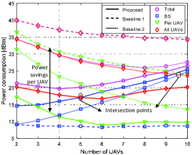
Figure 2: Power consumption versus number of UAVs, $L$.

Figure 3 illustrates the power consumption of the considered schemes as a function of the minimum rate achievable at the users, $R_{k}^{\min}$. From Figure 3 we observe that the power consumptions of both the UAVs and the ground BS increase monotonically with $R_{k}^{\min}$, as more transmit power is needed to simultaneously increase the rates for data transmission and fronthauling, cf. C5 and C6. Moreover, by optimizing the trajectories of the cooperating UAVs, the proposed scheme significantly reduces the power consumption per UAV for all considered $R_{k}^{\min}$s compared to the baseline schemes. To gain insight regarding the importance of optimal trajectory design, we note an interesting trade-off between the power consumptions for navigation and communication (including fronthauling and data transmission), which is revealed by Baseline Schemes 3 and 4, cf. the intersection points shown in the figure. In particular, for Baseline Scheme 3, the transmit power required by the ground BS for fronthauling is low as the UAVs hover close to the ground BS, whereas the UAVs may need a large power for data transmission, particularly when $R_{k}^{\min}$ is large, as they are far away from the users. In contrast, by having the UAVs fly close to the users (away from the ground BS), which leads to an increased navigation power, Baseline Scheme 4 reduces the power consumption required for data transmission when $R_{k}^{\min}$ is large, and the transmit power for fronthauling increases only slightly. Therefore, when $R_{k}^{\min}$ is large, flying the UAVs close to the users is preferable for lowing the UAVs’ power consumed in data transmission. On the other hand, when $R_{k}^{\min}$ is small, hovering the UAVs close to the ground BS is preferred for lowering the power consumption in navigation and fronthauling.

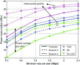
Figure 3: Power consumption versus users’ minimum required rate, $R_{k}^{\min}$.

VI Conclusions

In this paper, dynamic multi-UAV cooperation was investigated for enabling power-efficient aerial communications. Thereby, the UAVs are intelligently selected for cooperatively serving the ground users and the resulting large virtual array of moving antennas is exploited to reduce the power consumptions of UAV navigation and communication. The UAVs’ trajectories and cooperative beamforming were jointly designed by solving a mixed-integer non-convex optimization problem. As the problem is NP-hard, a low-complexity algorithm exploiting the underlying DC program structure was developed for finding a suboptimal solution. Simulation results revealed interesting trade-offs between the powers required for fronthauling, data transmission, and navigation in cooperative multi-UAV systems. Moreover, the proposed dynamic multi-UAV cooperation scheme can significantly lower the power consumption per UAV while guaranteeing the users’ QoS requirements, and hence, provides a promising approach to enhance aerial communications.

References

- [1] Y. Zeng, R. Zhang, and T. J. Lim, “Wireless communications with unmanned aerial vehicles: Opportunities and challenges,” IEEE Commun. Mag., vol. 54, no. 5, pp. 36–42, May 2016.
- [2] I. Bor-Yaliniz, M. Salem, G. Senerath, and H. Yanikomeroglu, “Is 5G ready for drones: A look into contemporary and prospective wireless networks from a standardization perspective,” IEEE Wireless Commun., vol. 26, no. 1, pp. 18–27, Feb. 2019.
- [3] H. Dihn-Tran, T. X. Vu, S. Chatzinotas, and B. Ottersten, “Energy-efficient trajectory design for UAV-enabled wireless communications with latency constraints,” in Asilomar Conf. Signals, Syst., Comput., Monterey, CA, Nov. 2019.
- [4] Q. Wu, Y. Zeng, and R. Zhang, “Joint trajectory and communication design for multi-UAV enabled wireless networks,” IEEE Trans. Wireless Commun., vol. 17, no. 3, pp. 2109–2121, Mar. 2018.
- [5] J. Zhang, H. Xu, L. Xiang, and J. Yang, “On the application of directional antennas in multi-tier unmanned aerial vehicle networks,” IEEE Access, vol. 7, pp. 132 095–132 110, 2019.
- [6] L. Liu, S. Zhang, and R. Zhang, “CoMP in the sky: UAV placement and movement optimization for multi-user communications,” arXiv preprint arXiv:1802.10371, Feb. 2018.
- [7] L. Liu, S. Zhang, and R. Zhang, “Multi-beam UAV communication in cellular uplink: Cooperative interference cancellation and sum-rate maximization,” IEEE Trans. Wireless Commun., vol. 18, no. 10, pp. 4679–4691, Oct. 2019.
- [8] X. Lin et al., “The sky is not the limit: LTE for unmanned aerial vehicles,” IEEE Commun. Mag., vol. 56, no. 4, pp. 204–210, Apr. 2018.
- [9] V. Yajnanarayana et al., “Interference mitigation methods for unmanned aerial vehicles served by cellular networks,” in IEEE 5G World Forum (5GWF), Dresden, Germany, Jul. 2018.
- [10] P. Marsch and G. P. Fettweis, Coordinated Multi-Point in Mobile Communications: From Theory to Practice. Cambridge University Press, 2011.
- [11] T. Lipp and S. Boyd, “Variations and extension of the convex–concave procedure,” Optimization and Engineering, vol. 17, no. 2, pp. 263–287, 2016.
- [12] D. Tse and P. Viswanath, Fundamentals of Wireless Communication. Cambridge University Press, 2005.
- [13] J. Seddon and S. Newman, Basic Helicopter Aerodynamics. American Institute of Aeronautics and Astronautics, 2001.
- [14] L. Xiang, D. W. K. Ng, R. Schober, and V. W. S. Wong, “Cache-enabled physical-layer security for video streaming in backhaul-limited cellular networks,” IEEE Trans. Wireless Commun., vol. 17, no. 2, pp. 736–751, Feb. 2018.
- [15] S. Boyd and L. Vandenberghe, Convex Optimization. Cambridge University Press, 2004.
- [16] 3GPP TR 36.814, “Further advancements for E-UTRA physical layer aspects (Release 9),” Mar. 2010.