Simulate forest trees by integrating L-system and 3D CAD files

Abstract

In this article, we propose a new approach for simulating trees, including their branches, sub-branches, and leaves. This approach combines the theory of biological development, mathematical models, and computer graphics, producing simulated trees and forest with full geometry. Specifically, we adopt the Lindenmayer process to simulate the branching pattern of trees and modify the available measurements and dimensions of 3D CAD developed object files to create natural looking sub-branches and leaves. Randomization has been added to the placement of all branches, sub branches and leaves. To simulate a forest, we adopt Inhomogeneous Poisson process to generate random locations of trees. Our approach can be used to create complex structured 3D virtual environment for the purpose of testing new sensors and training robotic algorithms. We look forward to applying this approach to test biosonar sensors that mimick bats’ fly in the simulated environment.

I Introduction

Thousands of years of biological evolution ultimately resulted in complex structured natural environments which play an important role for the survival of a wide variety of species and ecosystems [1]. The modeling of natural environments with forest trees has many theoretical and practical applications [2, 3], ranging from conceptual nature studies, to forest-based visual impact analysis and dynamic landscape synthesis for computer-based animation [4]. The inherent difficulty of tree modeling can be handled by using different approaches. For example, pioneering research methods for the efficient modeling of plant architecture have become available since 1971 [5, 6]. More recently, Reffye et. al [7] modeled plant growth and architectures by using stochastic processes combined with botanical analysis. For the three-dimensional (3D) modeling of individual trees, a number of methods have been proposed, including rule-based modelling [8], interactive parametric modelling [9], image-based 3D modelling [10], and 3D reconstruction based on plant structure data [11]. Software systems, such as the stand visualization system (SVS) [12], the forest vegetation simulator (FVS) [13], and Capsis [14], have been developed for the modeling and visualization of forest trees.

Despite these advances, existing tree models are still not sufficient for simulating the full geometry of forest trees. Tree models in available software often rely on plugins (for e.g: blender tree plugins). Moreover, simulating the full geometry of natural trees often involves far more parameters than those used in simplified tree models. Empirical tree models that are based on real tree templates are sometimes useful to construct natural looking trees. Additionally, due to the large variety of tree species, simulating tree structures of a large family of tree types is a challenging task.

In this paper, we propose an efficient approach for simulating natural looking trees by combining probabilistic models with empirical tree models. In particular, we integrate the commonly adopted Lindenmayer systems (L-systems) with 3D CAD object files, producing random tree architectures that look natural. The L-system [15] is a graphical model commonly used to define the branching patterns in trees and other organic forms [16]. It defines the branching pattern through recursively applying certain production rules on a string of symbols. Each symbol in the string defines a structural component (e.g., branch, terminal). Each recursive iteration creates an additional level of growth of the string. The final string represents the branching structure of the grown tree. While L-systems are commonly used to produce branching structures, they are not sufficient for generating natural looking trees in 3D because of over-simplified assumptions on the geometry of branches, sub-branches and leaves. We therefore further improve L-systems by including geometric structures available in 3D CAD developed object files. The randomization has been added in all branches, sub branches and leaves placements. This creates random trees with natural looks. To simulate a forest, we adopt Inhomogeneous Poisson process (IPP) to generate random locations of trees. The simulated forest is plotted in 3D for visualization. Our approach can be used to create complex structured 3D virtual environment for the purpose of testing new sensors and training robotic algorithms. We look forward to applying this approach to test biosonar sensors that mimick bats’ fly in the simulated environment.

The rest of this paper is organized as follows. In Section II, we describe in detail the methods for integrating L-system with 3D developed CAD files for the simulation of random trees, and discuss the random placement of trees in forest by sampling from the IPP. We elaborate the simulation results in Section III. Finally, in Section IV, a general conclusion and direction towards future work is given.

(a)

(b)

Figure 1: Tree model visualized in a CAD viewer. (left) A 3D model of a pine tree with trunk and branches. Triangular meshes can be seen in the zoomed in view. (right) Tree is visualized with the leafs, which are modeled as triangular meshes.

(a)

(b)

Figure 2: STL files displayed as 2D images. 2D images are generated by 3D rendering or visualization of the corresponding STL files.

II Materials and Methods

II-A The L-system approach

The biologist Aristid Lindenmayer [17] created a simultaneous rewriting framework in 1968, which uses a set of composition laws to regulate the evolution of a character string ($\omega$). This approach is now called the Lindenmayer (or L-System) system. L-System is initially used to provide a mathematical formalism for the creation of basic complex organisms like algae and fungi, and later expanded to mimic the complex branching systems of large plants found in nature. Further applications of L-System are also found in fields such as plant computer imaging. We now formally define an L-system.

Definition 1

An L-system G is a tuple $\textbf{G}=(A,\omega,P)$ where:

• $A$ is a finite set of symbols or variables that fall into 2 categories; (1) that can be replaced by other variables and (2) remains constant and cannot be replaced ;

• $\omega$ is a string of symbols from $V$ that defines the initial state of the system and is called the axiom;

• $P:A\rightarrow A^{\star}$ is the set of production rules that define how one variable transform into another. The predecessor is a single variable and the successor is a string from the set $A$.

The recursive nature of the L-System leads to self-similarity, therefore fractal-like and branched forms are easily generated. Plant models and other natural-looking forms are easily attained, as increasing the number of recursions causes the model to “grow” and generate a more complex self-similar structure. In our model, we start with an axiom and define a set of rules to describe branch structures as seen below:

$Variables:\ A=\{g,d\}$

$\{Axiom:\ \omega=\{g\}$

$Rule1:\ P(g)\rightarrow d(d)+d)[d(d)+d)$

$Rule2:\ P(g)\rightarrow d(d)+d)[d(d)+d)[d(d)+d)$

$Rule3:\ P(g)\rightarrow d(d)+d)[d(d)+d)[d(d)+d)[d(d)+d)$

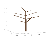
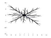
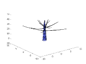
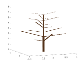
As seen above, we have 2 variables, where the variable $d$ is a constant and our axiom is the single character $g$. It is to be noted that different rules give rise to different branching patterns. For example, Rule 1 give rise to a tree with 6 branches and Rule 2 corresponds to a tree with 12 branches. This L-system can easily be extended and generally applied to create branch patterns. In Figure 3 (a), we demonstrate the plot of a simple tree with one level branching structure. As shown in Figure 3 (a), L-system only provides simplified branching structure. In order to simulate natural looking trees, more characteristics such as curvature of the branches need to be added. We achieve this by modify geometric information contained in CAD developed files.

II-B The CAD developed approach

Computer-aided design or CAD is a way of creating models of objects using computers. CAD software can be used to design both 2D and 3D object models, producing digital files that contain different parameters of the models. For example, a 3D model designed using CAD contains all details required to make a 3D print of the model. The 3D model is generally shown as a 2D image with 3D rendering or visualization. It is worth to note that, although the term 3D model refers to the object, the 3D file refers to both the object and the corresponding file type. A SolidWorks file and an STL file, for example, are both 3D files and can represent the same 3D object/model, but they do so differently and are thus different 3D files.

Regarding the representation, 3D models are often represented using the following formats: (1) a solid model that defines the volume occupied by the object, or (2) a surface representation model that models the surface of an object. Solid models are generally used for engineering analysis, for example, in limit load and failure analysis. Surface models, on the other hand, are commonly used in computer games and movies. An example of a surface model is an STL (STereoLithography) file. An STL file describes mesh surfaces as lists of geometric features. STL files contain polygonal meshes defined by vertices and normal vectors that represent the surface features of the 3D model. A solid surface is modeled as a composition of triangular faces, and each triangular face comprises a normal and the coordinates of the 3 vertices that form the triangle. The STL file stores information mostly in the binary form although a text representation can also be used.

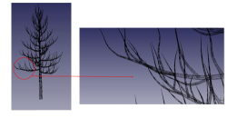
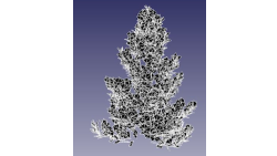
In the first step, the tree with adequate characteristic was chosen. The information obtained from the measurement of 3D CAD model has been used to visualize the object files of the trees in freeCAD software. An example is shown in Figure 1. The information about branches, sub-branches and leaves can be first extracted based on the coordinates and the meshes information from the object files. In second step, this information enables the placement of branches in accordance with the rules of L-system branching pattern. Since the coordinates of branches are available, we can randomize the angles and these geometry of these branches. The sub-branches can be added and modified by following the same steps. The leaves are then added by including the triangular meshes of leaves from object files, as shown in 2. The center point of each triangle is considered and randomized as per the change in angle of sub-branches.

II-C Inhomogenous Poisson process

Inhomogeneous Poisson Processes (IPPs) are flexible stochastic processes that model random points in space or random ”events” in a time interval. IPPs can be used to model a multitude of spatial and temporal phenomena, such as the number of cars passing through a junction or the timing/place of animal sightings. Based on a random tree simulator, we are able to generate a forest consisting of a random number of trees. By sampling from the IPP, we can determine the number of trees as well as the positions of these trees in a 2-D region.

Specifically, let $D\in\mathbb{R}^{2}$ denote the region in which the group of trees will be built. The random locations (i.e., $(x,y)$ coordinates) of the trees will be denoted by $S=\{s_{i},i=1,\dots,n\}$. We assume that S follows an IPP with intensity function $\lambda(s):D\rightarrow R^{+}$, where $\lambda(s)$ is a parameter that control the tree density on $D$. Small values of $\lambda(s)$ indicate sparse regions whereas high values indicate dense regions. Given the region $D$ and the intensity $\lambda(s)$, the number of trees, $n$, follows a Poisson distribution with mean $\int_{D}\lambda(s)ds$. To simulate $S$ given $n$, we adopt a thinning approach, and details can be found in [18].

III Simulation Results

(a)

(b)

(c)

(d)

Figure 3: Different stages of simulating a tree. (a) 8 different branches generated according to L-system rule. (b) The L-system model is used as a base to create a CAD, to mimic naturally occurring branches. (c) Sub-branches are added. (d) A top view of the final tree without leaves. The trunk, branches and sub-branches are modelled using triangular meshes.

(a)

(b)

(c)

(d)

Figure 4: Simulating a tree with 12 branches. (a) The branch locations and their orientation with respect to the trunk is seen. The branching pattern is in accordance with L-system rule 2. (b) 3D CAD model that mimics the L-system branching pattern. (c) Sub-branches added to the model. (d) Shows the complete 3D model with the leaves. Leaves are modelled as triangular meshes, but only the midpoint of the meshes are shown (green) for better visualization.

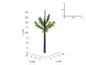
The primary intent of this study is develop a stochastic model to simulate random trees. We achieve this by integrating L-systems with CAD developed analytical tree models. In this section, we demonstrate results from several scenarios.

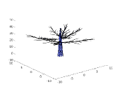
The first scenario is demonstrated in Figure 3. In this scenario, we simulate a tree with only eight branches. The starting points of the first level branches have been simulated using the L-system. The geometry about the branch lengths and sub-branches is obtained from the 3D developed CAD models.

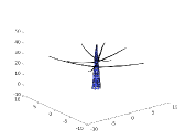
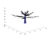
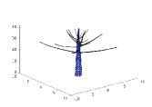
The second scenario is demonstrated in Figure 4. In this scenario, we simulate a random tree with 12 branches. The starting points of were simulated by using L-system. The branch lengths and sub-branches were then simulated by adopting the geometry of 3D developed CAD models. In this case, we added information about leaves, which is obtained by using the same geometry information of CAD model as shown in Figure 1. Each leaf is a triangular mesh, but only the center points of the leaves have been plotted.

We show the third scenario in Figure 5, which is similar to scenario 2, but with 16 branches simulated.

(a)

(b)

(c)

(d)

Figure 5: Different stages of simulating a tree with 16 branches.

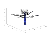
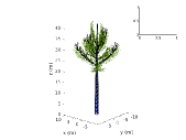
The above results demonstrate that it is feasible to simulate random trees with different number of branches, sub-branches and leaves. To simulate a forest with multiple trees, an IPP approach has been considered. Figure 6 shows the simulated locations of trees sampled from an IPP. Based on this results, we can generate multiple number of trees and plot them in a 3D environment.

(a)

(b)

(c)

(d)

Figure 6: Different number of trees sampled in a region to create a forest. The tree locations are sampled from an IPP. The number of trees in a region depend on the IPP parameter.

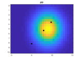
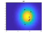
We further simulated forests with multiple trees. Results are plotted in Figure 7.

(a)

(b)

(c)

(d)

Figure 7: Simulating 2 trees in a region. (a)-(b) 3D model of the 2 trees with trunk and branches and their corresponding side view. (c)-(d) Sub-branches are now added and the side view are also visualized.

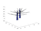
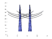
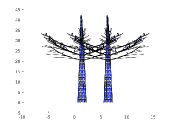
These plots demonstrate the effectiveness of our approach in generating natural looking trees in simulation environment. As many other 3D developed tree models are available online, our approach can be used to simulate a large community with different tree species. This work can be used in any application when a simulation model is needed for the testing of algorithms. For instance, one can simulate the motion of a robot in various scenarios such as obstacle avoidance and path following.

IV Conclusion

We have developed a new way of simulating and analysing 3D trees in simulated environment. By integrating the branching patterns generated by L-systems and the geometries of 3D CAD developed object files, our approach results in natural looking trees with full geometry about branches, sub-branches and leaves. Our approach also provides a way to simulate a forest by sampling the random locations of trees from an IPP model.

Our approach can be used to create complex structured 3D virtual environment for the purpose of testing new sensors and training robotic algorithms. One of the most prominent application of this research is the study of smart sonar sensors that mimic the biosonar system of bats. More than 800 species of echolocating bats use ultrasonic waves to detect their surroundings in forest. The highly efficient sonar systems of bats allow them to detect objects as thin as human hairs in complete darkness. They also enable them to efficiently navigate through dense vegetation by using echoes. To learn these impressive abilities from bats, it is imperative to simulate foliage echos data in a dense natural environment. Simulating real world trees is the first step towards achieving efficient navigation in forest. Future work, can be an extension of this work in robotic applications where a drone is flying with on board monocular camera and knowing the position of foliage using Inverse perspective mapping [19] and hence generating echos.

References

- [1] VINCENT RENOUF, OLIVIER CLAISSE, and ALINE Lonvaud-Funel. Understanding the microbial ecosystem on the grape berry surface through numeration and identification of yeast and bacteria. Australian Journal of Grape and Wine Research, 11(3):316–327, 2005.
- [2] Robert A Monserud. Simulation of forest tree mortality. Forest science, 22(4):438–444, 1976.
- [3] Jean-François Côté, Richard A Fournier, Joan E Luther, and Olivier R van Lier. Fine-scale three-dimensional modeling of boreal forest plots to improve forest characterization with remote sensing. Remote sensing of environment, 219:99–114, 2018.
- [4] Barbara Tversky, Julie Bauer Morrison, and Mireille Betrancourt. Animation: can it facilitate? International journal of human-computer studies, 57(4):247–262, 2002.
- [5] Hisao Honda. Description of the form of trees by the parameters of the tree-like body: Effects of the branching angle and the branch length on the shape of the tree-like body. Journal of Theoretical Biology, 31(2):331 – 338, 1971.
- [6] Jari Perttunen and Risto Sievänen. Incorporating lindenmayer systems for architectural development in a functional-structural tree model. Ecological modelling, 181(4):479–491, 2005.
- [7] Philippe De Reffye, François Houllier, Frédéric Blaise, Daniel Barthélémy, Jean Dauzat, and Daniel Auclair. A model simulating above-and below-ground tree architecture with agroforestry applications. Agroforestry systems, 30(1-2):175–197, 1995.
- [8] Bernd Lintermann and Oliver Deussen. Interactive modelling of branching structures. In SIGGRAPH 96: 23rd International Conference on Computer Graphics and Interactive Techniques, page 148, 1996.
- [9] Ludovic Hamon, Emmanuelle Richard, Paul Richard, Rachid Boumaza, and Jean-Louis Ferrier. Rtil-system: a real-time interactive l-system for 3d interactions with virtual plants. Virtual Reality, 16(2):151–160, 2012.
- [10] Thiago T Santos and Alberto A De Oliveira. Image-based 3d digitizing for plant architecture analysis and phenotyping. In Embrapa Informática Agropecuária-Artigo em anais de congresso (ALICE). In: CONFERENCE ON GRAPHICS, PATTERNS AND IMAGES, 25., 2012, Ouro Preto …, 2012.
- [11] Anthony Paproki, Xavier Sirault, Scott Berry, Robert Furbank, and Jurgen Fripp. A novel mesh processing based technique for 3d plant analysis. BMC plant biology, 12(1):63, 2012.
- [12] Robert J McGaughey. Visualizing forest stand dynamics using the stand visualization system. In Proceedings of the 1997 ACSM/ASPRS annual convention and exposition, volume 4, pages 248–257, 1997.
- [13] Nicholas L Crookston, Gerald E Rehfeldt, Gary E Dixon, and Aaron R Weiskittel. Addressing climate change in the forest vegetation simulator to assess impacts on landscape forest dynamics. Forest Ecology and Management, 260(7):1198–1211, 2010.
- [14] Samuel Dufour-Kowalski, Benoît Courbaud, Philippe Dreyfus, Céline Meredieu, and François De Coligny. Capsis: an open software framework and community for forest growth modelling. Annals of forest science, 69(2):221–233, 2012.
- [15] Takashi Ijiri, Shigeru Owada, and Takeo Igarashi. The sketch l-system: Global control of tree modeling using free-form strokes. In International Symposium on Smart Graphics, pages 138–146. Springer, 2006.
- [16] Przemyslaw Prusinkiewicz, Aristid Lindenmayer, and James Hanan. Developmental models of herbaceous plants for computer imagery purposes. Computer Graphics, 22(4):141–150, 1988.
- [17] Gabriela Ochoa. An introduction to lindenmayer systems. web site: http://www. cogs. susx. ac. uk/users/gabro/lsys/lsys. html, 1998.
- [18] Peter AW Lewis and Gerald S Shedler. Simulation of nonhomogeneous poisson processes with degree-two exponential polynomial rate function. Operations Research, 27(5):1026–1040, 1979.
- [19] M. Hassan Tanveer, Antonio Sgorbissa, and Antony Thomas. An ipm approach to multi-robot cooperative localization: Pepper humanoid and wheeled robots in a shared space. In Oleg Gusikhin and Kurosh Madani, editors, Informatics in Control, Automation and Robotics, pages 429–447, Cham, 2020. Springer International Publishing.