Rethinking Curriculum Learning with Incremental Labels and Adaptive Compensation

Abstract

Like humans, deep networks have been shown to learn better when samples are organized and introduced in a meaningful order or curriculum [Weinshall et al.(2018)Weinshall, Cohen, and Amir]. Conventional curriculum learning schemes introduce samples in their order of difficulty. This forces models to begin learning from a subset of the available data while adding the external overhead of evaluating the difficulty of samples. In this work, we propose Learning with Incremental Labels and Adaptive Compensation (LILAC), a two-phase method that incrementally increases the number of unique output labels rather than the difficulty of samples while consistently using the entire dataset throughout training. In the first phase, Incremental Label Introduction, we partition data into mutually exclusive subsets, one that contains a subset of the ground-truth labels and another that contains the remaining data attached to a pseudo-label. Throughout the training process, we recursively reveal unseen ground-truth labels in fixed increments until all the labels are known to the model. In the second phase, Adaptive Compensation, we optimize the loss function using altered target vectors of previously misclassified samples. The target vectors of such samples are modified to a smoother distribution to help models learn better. On evaluating across three standard image benchmarks, CIFAR-10, CIFAR-100, and STL-10, we show that LILAC outperforms all comparable baselines. Further, we detail the importance of pacing the introduction of new labels to a model as well as the impact of using a smooth target vector.

1 Introduction

Deep networks are a notoriously hard class of models to train effectively [Erhan et al.(2009)Erhan, Manzagol, Bengio, Bengio, and Vincent, Larochelle et al.(2007)Larochelle, Erhan, Courville, Bergstra, and Bengio, Glorot and Bengio(2010), Larochelle et al.(2009)Larochelle, Bengio, Louradour, and Lamblin]. A combination of high-dimensional problems, characterized by a large number of labels and a high volume of samples, a large number of free parameters and extreme sensitivity to experimental setups are some of the main reasons for the difficulty in training deep networks. The go-to solution for deep network optimization is Stochastic Gradient Descent with mini-batches [Robbins and Monro(1951)] (batch learning) or its derivatives. There are two alternative lines of work which offer strategies to guide deep networks to better solutions than batch learning: Curriculum Learning [Bengio et al.(2009)Bengio, Louradour, Collobert, and Weston, Florensa et al.(2017)Florensa, Held, Wulfmeier, Zhang, and Abbeel, Graves et al.(2017)Graves, Bellemare, Menick, Munos, and Kavukcuoglu] and Label Smoothing [Elman(1993), Xie et al.(2016)Xie, Wang, Wei, Wang, and Tian].

Curriculum learning helps deep networks learn better by gradually increasing the difficulty of samples used to train networks. This idea is inspired by methods used to teach humans and patterns in human cognition and behaviour [Skinner(1958), Avrahami et al.(1997)Avrahami, Kareev, Bogot, Caspi, Dunaevsky, and Lerner]. The “difficulty” of samples in the dataset, obtained using either external ranking methods or internal rewards [Hacohen and Weinshall(2019), Florensa et al.(2017)Florensa, Held, Wulfmeier, Zhang, and Abbeel], introduces an extra computational overhead while the setup itself restricts the amount of data from which the model begins to learn.

Label smoothing techniques [Xie et al.(2016)Xie, Wang, Wei, Wang, and Tian, Reed et al.(2015)Reed, Lee, Anguelov, Szegedy, Erhan, and Rabinovich, Pereyra et al.(2017)Pereyra, Tucker, Chorowski, Kaiser, and Hinton] regularize the outcomes of deep networks to prevent over-fitting while improving on existing solutions. They penalize network outputs based on criteria such as noisy labels, overconfident model outcomes, or robustness of a network around a data point in the feature space. Often, such methods penalize the entire dataset throughout the training phase with no regard to the prediction accuracy of each sample.

Figure 1: Illustration of the components of LILACfor a four label dataset case. The Incremental Label introduction (IL) phase introduces new labels at regular intervals while using the data corresponding to unknown labels (pseudo-label) as negative samples. Once all the labels have been introduced, the Adaptive Compensation (AC) phase of training begins. Here, a prior copy of the network is used to classify training data. If a sample is misclassified then a smoother distribution is used as its ground-truth vector in the current epoch.

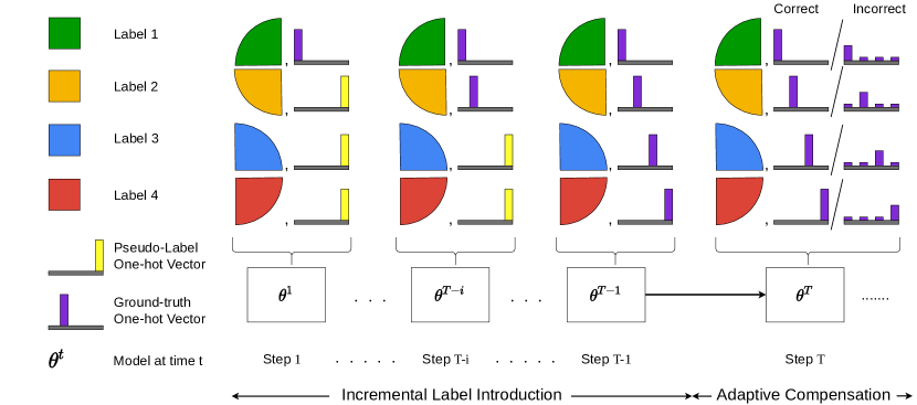
Inspired by an alternative outlook on Elman’s [Elman(1993)] notion of “starting small”, we propose LILAC, Learning with Incremental Labels and Adaptive Compensation, a novel label-based algorithm that overcomes the issues of the previous methods and effectively combines them. LILAC works in two phases, 1) Incremental Label Introduction (IL), which emphasizes gradually learning labels, instead of samples, and 2) Adaptive Compensation (AC), which regularizes the outcomes of previously misclassified samples by modifying their target vectors to smoother distributions in the objective function (Fig. 1).

In the first phase, we partition data into two mutually exclusive sets: $\mathbb{S}$, a subset of ground-truth (GT) labels and their corresponding data; and $\mathbb{U}$, remaining data associated with a pseudo-label ($\rho$) and used as negative samples. Once the network is trained using the current state of the data partition for a fixed interval, we reveal more GT labels and their corresponding data and repeat the training process. By contrasting data in $\mathbb{S}$ against the entire remaining dataset in $\mathbb{U}$, we consistently use all the available data throughout training, thereby overcoming one of the key issues of curriculum learning. The setup of the IL phase, inspired by continual learning, allows us to flexibly space out the introduction of new labels and provide the network enough time to develop a strong understanding of each class.

Once all the GT labels are revealed, we initiate the AC phase of training. In this phase, we replace the target one-hot vector of misclassified samples, obtained from a previous version of the network being trained, with a smoother distribution. The smoother distribution provides an easier value for the network to learn while the use of a prior copy of the network helps avoid external computational overhead and limits the alteration to only necessary samples.

To summarize, our main contributions in LILAC are as follows:

• we introduce a novel method for curriculum learning that incrementally learns labels as opposed to samples,

• we formulate Adaptive Compensation as a method to regularize misclassified samples while removing external computational overhead,

• finally, we improve average recognition accuracy across all of the evaluated benchmarks compared to batch learning, a property that is not shared by the other tested curriculum learning and label smoothing methods.

Our code is available at https://github.com/MichiganCOG/LILAC_v2.

2 Related Works

Curriculum Learning

Bengio et al [Bengio et al.(2009)Bengio, Louradour, Collobert, and Weston], Florensa et al [Florensa et al.(2017)Florensa, Held, Wulfmeier, Zhang, and Abbeel], and Graves et al [Graves et al.(2017)Graves, Bellemare, Menick, Munos, and Kavukcuoglu] are some important works that have redefined and applied curriculum learning in the context of deep networks. These ideas were expanded upon to show improvements in performance across corrupted [Jiang et al.(2018)Jiang, Zhou, Leung, Li, and Fei-Fei] and small datasets [Fan et al.(2018)Fan, Tian, Qin, Li, and Liu]. More recently, Hacohen and Weinshall [Hacohen and Weinshall(2019)] explored the impact of varying the pace with which samples were introduced while Weinshall [Weinshall et al.(2018)Weinshall, Cohen, and Amir] used alternative deep networks to categorize difficult samples. To the best of our knowledge, most previous works have assumed that samples cover a broad spectrum of difficulty and hence need to be categorized and presented in an orderly fashion. The closest relevant work to ours, in terms of learning labels, gradually varies the GT vector from a multimodal distribution to a one-hot vector over the course of the training phase [Dogan et al.(2019)Dogan, Deshmukh, Machura, and Igel].

Label Smoothing

Label smoothing techniques regularize deep networks by penalizing the objective function based on a pre-defined criterion. Such criteria include using a mixture of true and noisy labels [Xie et al.(2016)Xie, Wang, Wei, Wang, and Tian], penalizing highly confident outputs [Pereyra et al.(2017)Pereyra, Tucker, Chorowski, Kaiser, and Hinton], and using an alternate deep network’s outcomes as GT [Reed et al.(2015)Reed, Lee, Anguelov, Szegedy, Erhan, and Rabinovich]. Bagherinezhad et al [Bagherinezhad et al.(2018)Bagherinezhad, Horton, Rastegari, and Farhadi] proposed the idea of using logits from trained models instead of just one-hot vectors as GT. Complementary work by Miyato et al [Miyato et al.(2016)Miyato, Maeda, Koyama, Nakae, and Ishii] used the local distributional smoothness, based on the robustness of a model’s distribution around a data point, to smooth labels. The work closest to our method was proposed in Szegedy et al [Szegedy et al.(2016)Szegedy, Vanhoucke, Ioffe, Shlens, and Wojna], where an alternative target distribution was used across the entire dataset. Instead, we propose to alter the GT vector for only samples that are misclassified. They are identified using a prior copy of the current model, which helps avoid external computational overhead and only uses a small set of operations.

Incremental Learning and Negative Mining

Incremental and Continual learning are closely related fields that inspired the structure of our algorithm. Their primary concern is learning over evolving data distributions with the addition of constraints on the storage memory [Rebuffi et al.(2017)Rebuffi, Kolesnikov, Sperl, and Lampert, Castro et al.(2018)Castro, Marín-Jiménez, Guil, Schmid, and Alahari], distillation of knowledge across different distributions [Schwarz et al.(2018)Schwarz, Czarnecki, Luketina, Grabska-Barwinska, Teh, Pascanu, and Hadsell, Rolnick et al.(2019)Rolnick, Ahuja, Schwarz, Lillicrap, and Wayne], assumption of a single pass over data [Lopez-Paz and Ranzato(2017), Chaudhry et al.(2019)Chaudhry, Ranzato, Rohrbach, and Elhoseiny], etc. In our approach, we depart from the assumption of evolving data distributions. Instead, we adopt the experimental pipeline used in incremental learning to introduce new labels at regular intervals. At the same time, inspired by negative mining [Bucher et al.(2016)Bucher, Herbin, and Jurie, Li et al.(2013)Li, Snoek, Worring, Koelma, and Smeulders, Wang and Gupta(2015)], we use the remaining training data, associated with a pseudo-label, as negative samples. Overall, our setup effectively uses the entire training dataset, thus maintaining the same data distribution.

3 LILAC

In LILAC, our main objective is to improve upon batch learning. We do so by first gradually learning labels, in fixed increments, until all GT labels are known to the network (Section 3.1). This behaviour assumes that all samples are of equal difficulty and are available to the network throughout the training phase. Further, we focus on learning strong representations of each class over a dedicated period of time. Once all GT labels are known, we shift to regularizing previously misclassified samples by smoothing the distribution of their target vector while maintaining the peak at the same GT label (Section 3.2). Using a smoother distribution leads to an increase in the entropy of the target vector and helps the network learn better, as we demonstrate in Section 4.2.

Figure 2: Illustration of the steps in the IL phase when (Top) only one GT label is in $\mathbb{S}$ and (Bottom) when two GT labels are in $\mathbb{S}$. The steps are 1) partition data, 2) sample a mini-batch of data and 3) balance the number of samples from $\mathbb{U}$ to match those from $\mathbb{S}$ in the mini-batch before training. Samples from $\mathbb{U}$ are assumed to have a uniform prior when being augmented/reduced to match the total number of samples from $\mathbb{S}$. Values inside each pie represent the number of samples. Across both cases, the number of samples from $\mathbb{S}$ determines the final balanced mini-batch size.

3.1 Incremental Label Introduction Phase

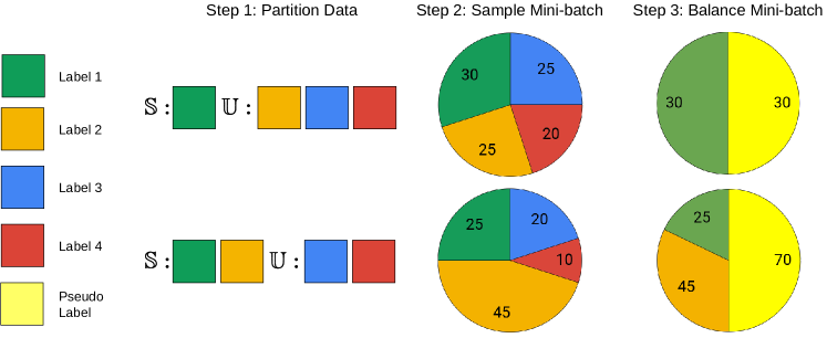
In the IL phase, we partition data into two sets: $\mathbb{S}$, a subset of GT labels and their corresponding data; and $\mathbb{U}$, the remaining data marked as negative samples using a pseudo-label $\rho$. Over the course of multiple intervals of training, we reveal more GT labels to the network according to a predetermined schedule. Within a given interval of training, the data partition is held fixed and we uniformly sample mini-batches from the entire training set based on their GT label. However, for samples from $\mathbb{U}$, we use $\rho$ as their label. There is no additional change required in the objective function or the outputs of the model when we sample data from $\mathbb{U}$. By the end of this phase, we reveal all GT labels to the network.

For a given dataset, we assume a total of $L$ labels are provided in the ascending order of their value. Based on this ordering, we initialize the first $b$ labels, and their corresponding data, as $\mathbb{S}$, and the data corresponding to the remaining $L-b$ labels as $\mathbb{U}$. Over the course of multiple training intervals, we reveal GT labels in increments of $m$, a hyper-parameter that controls the schedule of new label introduction. Revealing a GT label involves moving the corresponding data from $\mathbb{U}$ to $\mathbb{S}$ and using their GT label instead of $\rho$.

Within a training interval, we train the network for $E$ epochs using the current state of the data partition. First, we sample a mini-batch of data based on a uniform prior over their GT labels. Then, we modify their target vectors based on the partition to which a sample belongs. To ensure the balanced occurrence of samples from GT labels and $\rho$, we augment or reduce the number of samples from $\mathbb{U}$ to match those from $\mathbb{S}$ and use this curated mini-batch to train the network. After $E$ epochs, we move $m$ new GT labels and their corresponding data from $\mathbb{U}$ to $\mathbb{S}$ and repeat the entire process (Fig. 2).

3.2 Adaptive Compensation

Once all the GT labels have been revealed and the network has trained sufficiently, we begin the AC phase. In the AC phase, we use a smoother distribution for the target vector of samples which the network is unable to correctly classify. Compared to one-hot vectors, optimizing over this smoother distribution, with an increased entropy, can bridge the gap between the unequal distances in the embedding space and overlaps in the label space [Rodríguez et al.(2018)Rodríguez, Bautista, Gonzalez, and Escalera]. This overlap can occur due to common image content or close proximity in the embedding space relative to other classes. Thus, improving the entropy of such target vectors can help modify the embedding space in the next epoch and compensate for the predictions of misclassified samples.

For a sample $(x_{i},y_{i})$ in epoch $e\geq T$, we use predictions from the model at $e-1$ to determine the final target vector used in the objective function; specifically, we smoothen the target vector for a sample if and only if it was misclassified by the model at epoch $e-1$. Here, $(x_{i},y_{i})$ denotes a training sample and its corresponding GT label for sample index $i$, and $T$ represents a threshold epoch value until which the network is trained without adaptive compensation. We compute the final target vector for the $i^{th}$ instance at epoch $e$, $t_{i}^{e}$, based on the model $\theta^{e-1}$ using the following equation,

$$t_{i}^{e}=\begin{cases}(\frac{\epsilon L-1}{L-1})\delta_{y_{i}}+(\frac{1-\epsilon}{L-1})\mathbb{1},\quad\operatorname*{arg\,max}\big{(}f_{\theta^{e-1}}(x_{i})\big{)}\neq y_{i}\\ \delta_{y_{i}},\qquad\qquad\qquad\quad~{}~{}~{}\text{otherwise}\end{cases}.$$ (1)

Here, $\delta_{y_{i}}$ represents the one-hot vector corresponding to GT label $y_{i}$, $\mathbb{1}$ is a vector of $L$ dimensions with all entries as 1 and $\epsilon$ is a scaling hyper-parameter.

4 Experiments

Datasets and Metrics We use three datasets, CIFAR-10, CIFAR-100 ([Krizhevsky et al.(2009)Krizhevsky, Hinton, et al.]), and STL-10 ([Coates et al.(2011)Coates, Ng, and Lee]), to evaluate our method and validate our claims. CIFAR-10 and CIFAR-100 are 10 and 100 class variants of the popular image benchmark CIFAR while STL-10 is a 10 class subset of ImageNet. Average Recognition Accuracy (%) combined with their Standard Deviation across 5 trials are used to evaluate the performance of all the algorithms.

Experimental Setup For CIFAR-10/100, we use ResNet18 ([He et al.(2016)He, Zhang, Ren, and Sun]) as the architectural backbone while for STL-10, we use ResNet34. We set $\rho$ as the last label and $b$ as half the total number of labels of a given dataset. In each interval of LILAC’s IL phase, we train the model for 7, 3, and 10 epochs each, at a learning rate of 0.1, 0.01, and 0.1 for CIFAR-10, CIFAR-100, and STL-10, respectively. In the AC phase epochs 150, 220, and 370 are used as thresholds (epoch $T$) for CIFAR-10, CIFAR-100, and STL-10 respectively. Detailed explanations of the experimental setups are provided in the supplementary materials.

Baselines

1. Stochastic Gradient Descent with mini-batches (Batch Learning).

2. Standard Baselines

   • Fixed Curriculum: Following the methodology proposed in Bengio et al [Bengio et al.(2009)Bengio, Louradour, Collobert, and Weston], we create a “Simple” subset of the dataset using data that is within a value of 1.1 as predicted by a linear one-vs-all SVR model. The deep network is trained on the “Simple” dataset for a fixed period of time, which mirrors the total length of the IL phase, after which the entire dataset is used to train the network.

   • Label Smoothing: We follow the method proposed in Szegedy et al [Szegedy et al.(2016)Szegedy, Vanhoucke, Ioffe, Shlens, and Wojna].

3. Custom Baselines

   • Dynamic Batch Size (DBS): DBS randomly copies data available within a mini-batch to mimic variable batch sizes, similar to the IL phase. However, all GT labels are available to the model throughout the training process.

   • Random Augmentation (RA): This baseline samples from a single randomly chosen class in $\mathbb{U}$, available in the current mini-batch, to balance data between $\mathbb{S}$ and $\mathbb{U}$ in the current mini-batch. This is in contrast to LILAC, which uses samples from all classes in $\mathbb{U}$ that are available in the current mini-batch.

4. Ablative Baselines

   • Only IL: This baseline quantifies the contribution of incrementally learning labels when combined with batch learning.

   • Only AC: This baseline shows the impact of adaptive compensation, as a label smoothing technique, when combined with batch learning.

4.1 Comparison Against Standard Baselines

Table 1 illustrates the improvement offered by LILAC over Batch Learning, with comparable setups. Further, we break down the contributions of each phase of LILAC. Both Only IL and Only AC improve over batch learning, albeit to varying degrees, which highlights their individual strengths and importance. However, only when we combine both phases do we observe a consistently high performance across all benchmarks. This indicates that these two phases complement each other.

The Fixed Curriculum approach does not offer consistent improvements over the Batch Learning baseline across CIFAR-100 and STL-10 while the Label Smoothing approach does not outperform batch learning on the STL-10 dataset. While both of these standard baselines fall short, LILAC consistently outperforms Batch Learning across all evaluated benchmarks. Interestingly, Label Smoothing provides the highest performance on CIFAR-100. Since the original formulation of LILAC was based on Batch Learning, we assumed all GT vectors to be one-hot. This assumption is violated in Label Smoothing. When we tailor our GT vectors according to the Label Smoothing baseline, we outperform it with minimal hyper-parameter changes, a testament to LILAC’s applicability on top of conventional label smoothing.

Types	Training	Performance (%)
		CIFAR 10	CIFAR 100	STL 10
	Batch Learning	95.19 $\pm$ 0.190	78.32 $\pm$ 0.175	72.88 $\pm$ 0.642
Standard	Fixed Curriculum [Bengio et al.(2009)Bengio, Louradour, Collobert, and Weston]	95.27 $\pm$ 0.112	77.89 $\pm$ 0.287	72.18 $\pm$ 0.601
	Label Smoothing [Szegedy et al.(2016)Szegedy, Vanhoucke, Ioffe, Shlens, and Wojna]	95.27 $\pm$ 0.111	79.06 $\pm$ 0.179	72.55 $\pm$ 0.877
Custom	Random Augmentation	95.27 $\pm$ 0.076	75.37 $\pm$ 0.480	73.67 $\pm$ 0.708
	Dynamic Batch Size	95.22 $\pm$ 0.131	78.73 $\pm$ 0.264	72.66 $\pm$ 1.081
Ablative	Only IL (ours)	95.38 $\pm$ 0.135	78.73 $\pm$ 0.139	73.43 $\pm$ 0.903
	Only AC (ours)	95.38 $\pm$ 0.170	78.94 $\pm$ 0.179	72.94 $\pm$ 0.530
Overall	LILAC (ours)	95.52 $\pm$ 0.072	78.88 $\pm$ 0.201	73.77 $\pm$ 0.838
	LS + LILAC (ours)	95.34 $\pm$ 0.080	79.08 $\pm$ 0.307	73.59 $\pm$ 0.623

Table 1: Under similar setups, LILAC consistently achieves higher mean accuracy than Batch Learning across all evaluated benchmarks, a property not shared by other baselines.

Method	CIFAR-10
Wide Residual Networks [Zagoruyko and Komodakis(2016)]	96.11
Multilevel Residual Networks [Zhang et al.(2017)Zhang, Sun, Han, Yuan, Guo, and Liu]	96.23
Fractional Max-pooling [Graham(2014)]	96.53
Densely Connected Convolutional Networks [Huang et al.(2017)Huang, Liu, Van Der Maaten, and Weinberger]	96.54
Drop-Activation [Liang et al.(2018)Liang, Kwoo, and Yang]	96.55
Shake-Drop [Yamada et al.(2018)Yamada, Iwamura, Akiba, and Kise]	96.59
Shake-Drop + LILAC (ours)	96.79

Table 2: LILAC easily outperforms the Shake-Drop network ([Yamada et al.(2018)Yamada, Iwamura, Akiba, and Kise]) as well as other top performing algorithms on CIFAR-10 with standard pre-processing (random crop + flip).

The RA baseline highlights the importance of using all of the data in $\mathbb{U}$ as negative samples in the IL phase as opposed to using data from individual classes. This is reflected in the boost in performance offered by LILAC. The DBS baseline is used to highlight the importance of fluctuating mini-batch sizes, which occur due to the balancing of data in the IL phase. Even with the availability of all labels and fluctuating batch sizes, the DBS baseline is easily outperformed by LILAC. This indicates the importance of the recursive structure used to introduce data in the IL phase as well as the use of data from $\mathbb{U}$ as negative samples. Overall, LILAC consistently outperforms Batch Learning across all benchmarks while existing comparable methods fail to do so. When we extend LILAC to the Shake-Drop [Yamada et al.(2018)Yamada, Iwamura, Akiba, and Kise] network architecture, with only standard pre-processing, we easily outperform other existing approaches with comparable setups, as shown in Table 2.

4.2 Key Properties of LILAC

Smoothness of Target Vector ($\epsilon$)

Throughout this work, we maintained the importance of using a smoother distribution as the alternate target vector during the AC phase. Table 3 (Top) illustrates the change in performance across varying degrees of smoothness in the alternate target vector. There is a clear increase in performance when $\epsilon$ values are between 0.7-0.4 (mid-range). On either side of this band of values, the GT vector is either too sharp or too flat, leading to a drop in performance.

Size of Label Groups ($m$)

LILAC is designed to introduce as many or as few new labels as desired in the IL phase. We hypothesized that developing stronger representations can be facilitated by introducing a small number of new labels while contrasting it against a large variety of negative samples. Table 3 (Bottom) supports our hypothesis by illustrating the decrease in performance with an increase in the number of new labels introduced in each interval of the IL phase. Thus, we introduce two labels each for CIFAR-10 and STL-10 and only one new label per interval for CIFAR-100 throughout the experiments in Table 1.

Property	Performance (%)
	CIFAR-10	CIFAR-100	STL-10
$\epsilon=0.9$	95.30 $\pm$ 0.072	78.48 $\pm$ 0.328	73.57 $\pm$ 0.980
$\epsilon=0.8$	95.34 $\pm$ 0.141	78.52 $\pm$ 0.118	73.54 $\pm$ 0.984
$\epsilon=0.7$	95.42 $\pm$ 0.189	78.72 $\pm$ 0.356	73.59 $\pm$ 0.872
$\epsilon=0.6$	95.36 $\pm$ 0.096	78.75 $\pm$ 0.180	73.77 $\pm$ 0.838
$\epsilon=0.5$	95.49 $\pm$ 0.207	78.88 $\pm$ 0.227	73.61 $\pm$ 0.810
$\epsilon=0.4$	95.52 $\pm$ 0.072	78.88 $\pm$ 0.201	73.54 $\pm$ 0.959
$\epsilon=0.3$	95.31 $\pm$ 0.125	78.66 $\pm$ 78.66	73.59 $\pm$ 0.955
$\epsilon=0.2$	95.36 $\pm$ 0.095	78.47 $\pm$ 0.093	73.57 $\pm$ 0.963
$m$: 1	95.32 $\pm$ 0.156	78.73 $\pm$ 0.139	73.27 $\pm$ 0.220
$m$: 2 (4)	95.38 $\pm$ 0.135	78.34 $\pm$ 0.209	73.43 $\pm$ 0.903
$m$: 4 (8)	95.29 $\pm$ 0.069	78.37 $\pm$ 0.114	72.30 $\pm$ 0.543

Table 3: (Top) The mid-range of $\epsilon$ values, 0.7-0.4, show an increase in performance while the edges, due to either too sharp or too flat a distribution, show decreased performance. (Bottom) Only IL model results illustrate the importance of introducing a small number of new labels in each interval of the IL phase. Values in brackets are for CIFAR-100.

5 Discussion: Impact of Each Phase

In this section, we take a closer look at the impact of each phase of LILAC and how they affect the quality of the learned representations. We extract features from the second to last layer of ResNet18/34 from 3 different baselines (Batch Learning, LILAC, and Only IL) and use these features to train a linear SVM model.

Fig. 3 highlights the two important phases in our algorithm. First, the plots on the left-hand side show a steady improvement in the performance of LILAC and the Only IL baseline once the IL phase is complete and all the labels have been introduced to the network. When we compare the plots of CIFAR-10 and STL-10 against CIFAR-100, we see that all baselines follow the learning trend shown by Batch Learning, with CIFAR-100 being slightly delayed. Since there are a large number of epochs required to introduce all the labels of CIFAR-100 to the network, the plots are significantly delayed compared to batch learning. Conversely, since there are very few epochs in the IL phase of CIFAR-10 and STL-10, we observe the performance trend of Only IL and LILAC quickly match that of Batch Learning. Overall, the final performances of both LILAC and the Only IL baseline are higher than Batch Learning, which supports the importance of the IL phase in learning strong representations.

Figure 3: Plots on the (Left) show the common learning trend between all baselines, albeit slightly delayed for CIFAR-100, after the IL phase while those on the (Right) show steady improvement in performance after applying AC when compared to the Only IL baseline. Final supervised classification performances on representations collected from LILAC easily outperform those from Batch Learning and Only IL methods.

(a) CIFAR-10

(b) CIFAR-100

(c) STL-10

Figure 4: Illustration of 8 randomly chosen samples that were incorrectly labelled by the Only IL baseline and correctly labelled by LILAC. This highlights the importance of AC.

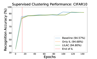
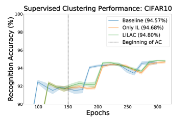
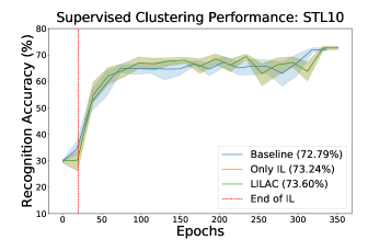
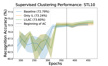
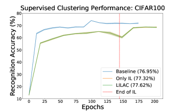
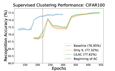
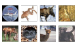
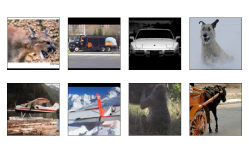
The plots on the right-hand side highlight the similarity in behaviour of Only IL and LILAC before AC. However, afterward, we observe that the performance of LILAC overtakes the Only IL baseline. This is a clear indicator of the improvement in representation quality when AC is applied. Additionally, from Fig. 3 we observe that inherently the STL-10 dataset results have a high standard deviation, which is reflected in the middle portion of the training phase, between the end of IL and the beginning of AC and it is not a consequence of our approach. We provide examples in Fig. 4 of randomly sampled data from the testing set that were incorrectly classified by the Only IL baseline and were correctly classified by LILAC.

6 Conclusion

In this work, we proposed LILAC, which rethinks curriculum learning based on incrementally learning labels instead of samples. This approach helps kick-start the learning process from a substantially better starting point while making the learned embedding space amenable to adaptive compensation of target vectors. Both these techniques combine well in LILAC to show the highest performance on CIFAR-10 for simple data augmentations while easily outperforming batch and curriculum learning and label smoothing methods on comparable network architectures. The next step in unlocking the full potential of this setup is to include a confidence measure on the predictions of the network so that it can handle the effects of dropout or partial inputs. In further expanding LILAC’s ability to handle partial inputs, we aim to explore its effect on standard incremental learning (memory-constrained) while also extending its applicability to more complex neural network architectures.

7 Acknowledgements

This work was in part supported by NSF NRI IIS 1522904 and NIST 60NANB17D191. The findings and views represent those of the authors alone and not the funding agencies. The authors would also like to thank members of the COG lab for their invaluable input in putting together and refining this work.

Appendix A Experimental Setup

In Table 4 we list the general hyper-parameters used to train the batch learning portion of every baseline. This setup covers the training beyond the IL phase for LILAC, DBS, RA, and Only IL as well as the Only AC baseline. Across all the methods we ensure that the total number of training epochs, when all the labels in the dataset are known, is held constant.

Parameters	CIFAR10/100	STL10
Epochs	300	450
Batch Size	128	128
Learning Rate	0.1	0.1
Lr Milestones	[90 180 260]	[300 400]
Weight Decay	0.0005	0.0005
Nesterov Momentum	Yes	Yes
Gamma	0.2	0.1

Table 4: List of hyper-parameters used to in batch learning. Note: All experiments used the SGD optimizer.

Appendix B Hyper-parameter Selection

Property	Performance (%)
	CIFAR-10	CIFAR-100	STL-10
$E=1$	95.13 $\pm$ 0.175	78.21 $\pm$ 0.236	72.59 $\pm$ 0.476
$E=3$	95.20 $\pm$ 0.200	78.73 $\pm$ 0.139	73.03 $\pm$ 0.380
$E=5$	95.32 $\pm$ 0.044	78.57 $\pm$ 0.102	73.08 $\pm$ 0.996
$E=7$	95.32 $\pm$ 0.156	78.44 $\pm$ 0.265	73.13 $\pm$ 1.460
$E=10$	95.26 $\pm$ 0.185	77.98 $\pm$ 0.218	73.27 $\pm$ 0.220
Label Order: Rnd.	95.30 $\pm$ 0.146	78.35 $\pm$ 0.280	73.10 $\pm$ 0.861
Label Order: Difficulty	95.25 $\pm$ 0.156	78.42 $\pm$ 0.115	73.69 $\pm$ 0.849
Label Order: Asc.	95.32 $\pm$ 0.156	78.73 $\pm$ 0.139	73.27 $\pm$ 0.220

Table 5: (Top) Varying $E$, the fixed training interval size in the IL phase, shows a dataset specific behaviour, with the dataset with lesser labels preferring a larger number of epochs while the dataset with more labels prefers a smaller number of epochs. (Bottom) Comparing random label ordering and difficulty-based label ordering to the ascending order assumption used throughout our experiments, we observe no preference to any ordering pattern.

Figure 5: Unsupervised classification performance on representations collected from LILAC easily outperforms those collected from Batch Learning and Only IL methods. The plots on the left show the common learning trend between all baselines after IL while plots on the right show steady improvement in performance after applying AC when compared to the baselines.

Epochs in Training Interval

When we vary $E$, the fixed training interval size in the IL phase, we observe a dataset specific behaviour. For datasets with lesser number of total labels, a larger number of epochs provides better performance while for datasets with more labels, a smaller number of epochs yields better performance. While the alternate learning rate can have a huge impact on this performance, pacing the introduction of new labels, according to the empirical results, can have a tremendous impact on subsequent hyper-parameters used in LILAC.

Label Order

In Table 5, we compare three different orders of label introduction during the IL phase, 1) random label order, 2) difficulty-based label order, and 3) ascending label order. Here, difficulty-based label order is obtained from the overall classification scores per label, obtained from the features of a trained model. Although these three orders do not constitute the exhaustive set of possible label orderings, within these three possibilities there is no definitive order that boosts the performance of LILAC consistently. Thus, we employ ascending label order throughout our work.

NOTE: Only IL baseline is used throughout Table 5.

Appendix C Extended Results for Discussion: Impact of Each Phase

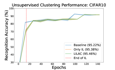
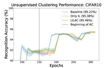
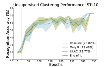
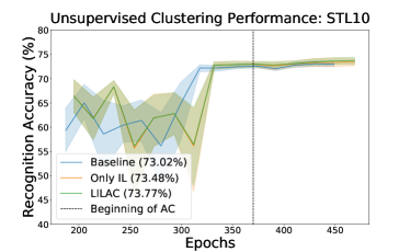
We include unsupervised clustering performance for CIFAR-10 and STL-10 using the k-means and the hungarian job assignment algorithm [Kuhn(1955)] in Fig. 5. They follow similar patterns to their supervised counterparts.

References

- [Avrahami et al.(1997)Avrahami, Kareev, Bogot, Caspi, Dunaevsky, and Lerner] Judith Avrahami, Yaakov Kareev, Yonatan Bogot, Ruth Caspi, Salomka Dunaevsky, and Sharon Lerner. Teaching by examples: Implications for the process of category acquisition. The Quarterly Journal of Experimental Psychology Section A, 50(3):586–606, 1997.
- [Bagherinezhad et al.(2018)Bagherinezhad, Horton, Rastegari, and Farhadi] Hessam Bagherinezhad, Maxwell Horton, Mohammad Rastegari, and Ali Farhadi. Label refinery: Improving imagenet classification through label progression. arXiv preprint arXiv:1805.02641, 2018.
- [Bengio et al.(2009)Bengio, Louradour, Collobert, and Weston] Yoshua Bengio, Jérôme Louradour, Ronan Collobert, and Jason Weston. Curriculum learning. In Proceedings of the 26th annual international conference on machine learning, pages 41–48. ACM, 2009.
- [Bucher et al.(2016)Bucher, Herbin, and Jurie] Maxime Bucher, Stéphane Herbin, and Frédéric Jurie. Hard negative mining for metric learning based zero-shot classification. In Gang Hua and Hervé Jégou, editors, Computer Vision – ECCV 2016 Workshops, pages 524–531, Cham, 2016. Springer International Publishing. ISBN 978-3-319-49409-8.
- [Castro et al.(2018)Castro, Marín-Jiménez, Guil, Schmid, and Alahari] Francisco M Castro, Manuel J Marín-Jiménez, Nicolás Guil, Cordelia Schmid, and Karteek Alahari. End-to-end incremental learning. In Proceedings of the European Conference on Computer Vision (ECCV), pages 233–248, 2018.
- [Chaudhry et al.(2019)Chaudhry, Ranzato, Rohrbach, and Elhoseiny] Arslan Chaudhry, Marc’Aurelio Ranzato, Marcus Rohrbach, and Mohamed Elhoseiny. Efficient lifelong learning with a-GEM. In International Conference on Learning Representations, 2019.
- [Coates et al.(2011)Coates, Ng, and Lee] Adam Coates, Andrew Ng, and Honglak Lee. An analysis of single-layer networks in unsupervised feature learning. In Proceedings of the fourteenth international conference on artificial intelligence and statistics, pages 215–223, 2011.
- [Dogan et al.(2019)Dogan, Deshmukh, Machura, and Igel] Urun Dogan, Aniket Anand Deshmukh, Marcin Machura, and Christian Igel. Label-similarity curriculum learning. arXiv preprint arXiv:1911.06902, 2019.
- [Elman(1993)] Jeffrey L Elman. Learning and development in neural networks: The importance of starting small. Cognition, 48(1):71–99, 1993.
- [Erhan et al.(2009)Erhan, Manzagol, Bengio, Bengio, and Vincent] Dumitru Erhan, Pierre-Antoine Manzagol, Yoshua Bengio, Samy Bengio, and Pascal Vincent. The difficulty of training deep architectures and the effect of unsupervised pre-training. In Artificial Intelligence and Statistics, pages 153–160, 2009.
- [Fan et al.(2018)Fan, Tian, Qin, Li, and Liu] Yang Fan, Fei Tian, Tao Qin, Xiang-Yang Li, and Tie-Yan Liu. Learning to teach. In International Conference on Learning Representations, 2018.
- [Florensa et al.(2017)Florensa, Held, Wulfmeier, Zhang, and Abbeel] Carlos Florensa, David Held, Markus Wulfmeier, Michael Zhang, and Pieter Abbeel. Reverse curriculum generation for reinforcement learning. In Proceedings of the 1st Annual Conference on Robot Learning, volume 78 of Proceedings of Machine Learning Research, pages 482–495. PMLR, 13–15 Nov 2017.
- [Glorot and Bengio(2010)] Xavier Glorot and Yoshua Bengio. Understanding the difficulty of training deep feedforward neural networks. In Proceedings of the thirteenth international conference on artificial intelligence and statistics, pages 249–256, 2010.
- [Graham(2014)] Ben Graham. Fractional max-pooling (2014). arXiv preprint arXiv:1412.6071, 2014.
- [Graves et al.(2017)Graves, Bellemare, Menick, Munos, and Kavukcuoglu] Alex Graves, Marc G Bellemare, Jacob Menick, Remi Munos, and Koray Kavukcuoglu. Automated curriculum learning for neural networks. In Proceedings of the 34th International Conference on Machine Learning-Volume 70, pages 1311–1320. JMLR. org, 2017.
- [Hacohen and Weinshall(2019)] Guy Hacohen and Daphna Weinshall. On the power of curriculum learning in training deep networks. In Proceedings of the 36th International Conference on Machine Learning, Proceedings of Machine Learning Research, pages 2535–2544, Long Beach, California, USA, 09–15 Jun 2019. PMLR.
- [He et al.(2016)He, Zhang, Ren, and Sun] Kaiming He, Xiangyu Zhang, Shaoqing Ren, and Jian Sun. Deep residual learning for image recognition. In Proceedings of the IEEE conference on computer vision and pattern recognition, pages 770–778, 2016.
- [Huang et al.(2017)Huang, Liu, Van Der Maaten, and Weinberger] Gao Huang, Zhuang Liu, Laurens Van Der Maaten, and Kilian Q Weinberger. Densely connected convolutional networks. In Proceedings of the IEEE conference on computer vision and pattern recognition, pages 4700–4708, 2017.
- [Jiang et al.(2018)Jiang, Zhou, Leung, Li, and Fei-Fei] Lu Jiang, Zhengyuan Zhou, Thomas Leung, Li-Jia Li, and Li Fei-Fei. MentorNet: Learning data-driven curriculum for very deep neural networks on corrupted labels. In Proceedings of the 35th International Conference on Machine Learning, Proceedings of Machine Learning Research, pages 2304–2313. PMLR, 10–15 Jul 2018.
- [Krizhevsky et al.(2009)Krizhevsky, Hinton, et al.] Alex Krizhevsky, Geoffrey Hinton, et al. Learning multiple layers of features from tiny images. Technical report, Citeseer, 2009.
- [Kuhn(1955)] Harold W Kuhn. The hungarian method for the assignment problem. Naval research logistics quarterly, 2(1-2):83–97, 1955.
- [Larochelle et al.(2007)Larochelle, Erhan, Courville, Bergstra, and Bengio] Hugo Larochelle, Dumitru Erhan, Aaron Courville, James Bergstra, and Yoshua Bengio. An empirical evaluation of deep architectures on problems with many factors of variation. In Proceedings of the 24th international conference on Machine learning, pages 473–480. ACM, 2007.
- [Larochelle et al.(2009)Larochelle, Bengio, Louradour, and Lamblin] Hugo Larochelle, Yoshua Bengio, Jérôme Louradour, and Pascal Lamblin. Exploring strategies for training deep neural networks. Journal of machine learning research, 10(Jan):1–40, 2009.
- [Li et al.(2013)Li, Snoek, Worring, Koelma, and Smeulders] Xirong Li, CeesG M Snoek, Marcel Worring, Dennis Koelma, and Arnold WM Smeulders. Bootstrapping visual categorization with relevant negatives. IEEE Transactions on Multimedia, 15(4):933–945, 2013.
- [Liang et al.(2018)Liang, Kwoo, and Yang] Senwei Liang, Yuehaw Kwoo, and Haizhao Yang. Drop-activation: Implicit parameter reduction and harmonic regularization. arXiv preprint arXiv:1811.05850, 2018.
- [Lopez-Paz and Ranzato(2017)] David Lopez-Paz and Marc’Aurelio Ranzato. Gradient episodic memory for continual learning. In Advances in Neural Information Processing Systems, pages 6467–6476, 2017.
- [Miyato et al.(2016)Miyato, Maeda, Koyama, Nakae, and Ishii] Takeru Miyato, Shin-ichi Maeda, Masanori Koyama, Ken Nakae, and Shin Ishii. Distributional smoothing by virtual adversarial examples. In 4th International Conference on Learning Representations, ICLR 2016, San Juan, Puerto Rico, May 2-4, 2016, Conference Track Proceedings, 2016.
- [Pereyra et al.(2017)Pereyra, Tucker, Chorowski, Kaiser, and Hinton] Gabriel Pereyra, George Tucker, Jan Chorowski, Lukasz Kaiser, and Geoffrey E. Hinton. Regularizing neural networks by penalizing confident output distributions. CoRR, 2017.
- [Rebuffi et al.(2017)Rebuffi, Kolesnikov, Sperl, and Lampert] Sylvestre-Alvise Rebuffi, Alexander Kolesnikov, Georg Sperl, and Christoph H Lampert. icarl: Incremental classifier and representation learning. In Proceedings of the IEEE conference on Computer Vision and Pattern Recognition, pages 2001–2010, 2017.
- [Reed et al.(2015)Reed, Lee, Anguelov, Szegedy, Erhan, and Rabinovich] Scott E. Reed, Honglak Lee, Dragomir Anguelov, Christian Szegedy, Dumitru Erhan, and Andrew Rabinovich. Training deep neural networks on noisy labels with bootstrapping. In 3rd International Conference on Learning Representations, ICLR 2015, San Diego, CA, USA, May 7-9, 2015, Workshop Track Proceedings, 2015.
- [Robbins and Monro(1951)] Herbert Robbins and Sutton Monro. A stochastic approximation method. The annals of mathematical statistics, pages 400–407, 1951.
- [Rodríguez et al.(2018)Rodríguez, Bautista, Gonzalez, and Escalera] Pau Rodríguez, Miguel A Bautista, Jordi Gonzalez, and Sergio Escalera. Beyond one-hot encoding: Lower dimensional target embedding. Image and Vision Computing, 75:21–31, 2018.
- [Rolnick et al.(2019)Rolnick, Ahuja, Schwarz, Lillicrap, and Wayne] David Rolnick, Arun Ahuja, Jonathan Schwarz, Timothy Lillicrap, and Gregory Wayne. Experience replay for continual learning. In Advances in Neural Information Processing Systems, pages 348–358, 2019.
- [Schwarz et al.(2018)Schwarz, Czarnecki, Luketina, Grabska-Barwinska, Teh, Pascanu, and Hadsell] Jonathan Schwarz, Wojciech Czarnecki, Jelena Luketina, Agnieszka Grabska-Barwinska, Yee Whye Teh, Razvan Pascanu, and Raia Hadsell. Progress & compress: A scalable framework for continual learning. In International Conference on Machine Learning, pages 4535–4544, 2018.
- [Skinner(1958)] Burrhus F Skinner. Reinforcement today. American Psychologist, 13(4):94, 1958.
- [Szegedy et al.(2016)Szegedy, Vanhoucke, Ioffe, Shlens, and Wojna] Christian Szegedy, Vincent Vanhoucke, Sergey Ioffe, Jon Shlens, and Zbigniew Wojna. Rethinking the inception architecture for computer vision. In Proceedings of the IEEE conference on computer vision and pattern recognition, pages 2818–2826, 2016.
- [Wang and Gupta(2015)] Xiaolong Wang and Abhinav Gupta. Unsupervised learning of visual representations using videos. In Proceedings of the IEEE International Conference on Computer Vision, pages 2794–2802, 2015.
- [Weinshall et al.(2018)Weinshall, Cohen, and Amir] Daphna Weinshall, Gad Cohen, and Dan Amir. Curriculum learning by transfer learning: Theory and experiments with deep networks. In Proceedings of the 35th International Conference on Machine Learning, Proceedings of Machine Learning Research, pages 5238–5246, Stockholmsmässan, Stockholm Sweden, 2018. PMLR.
- [Xie et al.(2016)Xie, Wang, Wei, Wang, and Tian] Lingxi Xie, Jingdong Wang, Zhen Wei, Meng Wang, and Qi Tian. Disturblabel: Regularizing cnn on the loss layer. In Proceedings of the IEEE Conference on Computer Vision and Pattern Recognition, pages 4753–4762, 2016.
- [Yamada et al.(2018)Yamada, Iwamura, Akiba, and Kise] Yoshihiro Yamada, Masakazu Iwamura, Takuya Akiba, and Koichi Kise. Shakedrop regularization for deep residual learning. arXiv preprint arXiv:1802.02375, 2018.
- [Zagoruyko and Komodakis(2016)] Sergey Zagoruyko and Nikos Komodakis. Wide residual networks. In British Machine Vision Conference 2016. British Machine Vision Association, 2016.
- [Zhang et al.(2017)Zhang, Sun, Han, Yuan, Guo, and Liu] Ke Zhang, Miao Sun, Tony X Han, Xingfang Yuan, Liru Guo, and Tao Liu. Residual networks of residual networks: Multilevel residual networks. IEEE Transactions on Circuits and Systems for Video Technology, 28(6):1303–1314, 2017.