Infinite ergodic theory meets Boltzmann statistics

Abstract

We investigate the overdamped stochastic dynamics of a particle in an asymptotically flat external potential field, in contact with a thermal bath. For an infinite system size, the particles may escape the force field and diffuse freely at large length scales. The partition function diverges and hence the standard canonical ensemble fails. This is replaced with tools stemming from infinite ergodic theory. Boltzmann-Gibbs statistics, even though not normalized, still describes integrable observables, like energy and occupation times. The Boltzmann infinite density is derived heuristically using an entropy maximization principle, as well as via a first-principles calculation using an eigenfunction expansion in the continuum of low-energy states. A generalized virial theorem is derived, showing how the virial coefficient describes the delay in the diffusive spreading of the particles, found at large distances. When the process is non-recurrent, e.g. diffusion in three dimensions with a Coulomb-like potential, we use weighted time averages to restore basic canonical relations between time and ensemble averages.

I Introduction

The overdamped stochastic dynamics of a particle in an external potential field ${V(x)}$, in one dimension, in contact with a thermal bath, is given by the Langevin equation

$${\textrm{d}x\over{\textrm{d}t}}=-{V^{\prime}(x)\over\gamma}+\sqrt{2D}\eta(t).$$ (1)

Here $-V^{\prime}(x)$ is the deterministic force applied on the particle due to the potential field, and $\gamma>0$ is the friction constant. $\eta(t)$ is the bath noise, which is white, Gaussian, has zero mean and $\langle\eta(t)\eta(t^{\prime})\rangle=\delta(t-t^{\prime})$ (where $\delta(\cdot)$ is the Dirac ${\delta}$-function). The Einstein relation $D=k_{B}T/\gamma$ guarantees that the system, in the case of a binding potential $V(x)$, will relax to thermal equilibrium. In this case, the steady-state equilibrium density is Chandler [1987]

$$P_{{\rm eq}}(x)={\exp\left[-V(x)/k_{B}T\right]\over Z}.$$ (2)

This final equilibrium state transcends a particular type of dynamics, and the asymptotic shape of the density does not depend on transport coefficients, such as the diffusion constant $D$, of the particles in the medium. Here,

$$Z=\int_{-\infty}^{\infty}\exp\left[-V(x)/k_{B}T\right]{\rm d}x$$ (3)

is the normalizing partition function, and $k_{B}$ is the Boltzmann constant.

A finite value of $Z$ is, however, not always guaranteed. In particular, $Z$ can diverge when $V(x)$ generates a force $F(x)=-V^{\prime}(x)\to 0$ when ${x\rightarrow\infty}$ and/or ${-\infty}$. More specifically, in this manuscript we are interested in the case where ${V(x)}$ itself drops to zero at large distance, at least as fast as ${1/x}$. We initiated a study of this case in a previous work Aghion, Kessler, and Barkai [2019], finding that at long times, and finite ${x}$, the time-dependent density assumes the shape of the Boltzmann-Gibbs factor, multiplied by a factor which decays as power-law in time. In the limit ${t\rightarrow\infty}$, the Boltzmann-Gibbs factor becomes an infinite-invariant density Aghion, Kessler, and Barkai [2019]. In the potential-free region, the density is simply the free-diffusion kernel. The appearance of the Boltzmann-Gibbs density can be understood as resulting from the fact that the particle returns infinitely many times to the potential region and so a kind of conditioned equilibrium is established there. In addition, we then showed in Aghion, Kessler, and Barkai [2019] how in this thermal setting, we recover the Aaronson-Darling-Kac theorem Darling and Kac [1957]; Aaronson [1997], which describes the ergodic properties of a certain class of observables, integrable with respect to the infinite density. In the current work, we extend our previous study in several directions. Most notably, we re-derive our previous (one-dimensional) results using an eigenfunction expansion of the relevant time-dependent Fokker-Planck equation and thereby not only succeed in recovering the infinite-invariant density, but the leading-order corrections as well. We also derive a virial theorem for our system, and extend some of our results to ${d\geq 1}$ dimensions.

There are many other situations where ${Z}$ diverges as well. Some examples are presented in Fig. 1, to be compared with the binding potential Fig. 1a which leads to finite ${Z}$. For logarithmic potentials, such as the example in Fig. 1b, the partition function diverges when the depth of the well is sufficiently shallow. This happens when ${V(x)\sim V_{0}\log(|x|)}$ at large ${|x|}$, and ${V_{0}<k_{B}T}$ at a certain given temperature, and the infinite invariant density of this class of potentials was studied in Dechant et al. [2011]; Aghion, Kessler, and Barkai [2019]; Bouin, Dolbeault, and Schmeiser [2020]). In addition, one may consider other non-binding fields, for example periodic structures, Fig. 1e, random potentials, or unstable fields, Fig. 1f. All the examples c-e share two properties: first, the partition function diverges, and second, the Langevin dynamics is recurrent in one dimension. In turn, in one dimension this implies that the mean return time in these examples is diverging. We will refer to the class of potentials which fulfill these conditions as weakly binding. Logarithmic potentials are a marginal case, which behaves as binding or weakly binding given the system parameters, and the unstable potential in Fig. 1f belongs to neither group. As will become clear below, while binding potentials lead to standard ergodic theory, we anticipate that infinite ergodic theory will serve as a useful tool for Langevin dynamics in one dimension for all the weakly binding potentials (though as mentioned, in this work we study in detail only asymptotically flat fields). Note that the extension of the theory to higher dimensions is not only a technical issue, since in that case the random walk is no longer recurrent. The basic tools to deal with this case need some modifications, as we demonstrate for isotropic potentials whose amplitude drops to zero at large radial distances ${r}$, at least as fast as ${1/r}$, below.

Figure 1: Various classes of potential landscapes: a. An example of a binding potential; ${V(x)\sim x^{2}}$. Here, the standard Boltzmann-Gibbs equilibrium state is achieved in the long-time limit, and standard ergodic theory applies. b. A logarithmic potential, ${V(x)\sim\log(|x|)}$ for ${|x|\gg 1}$; here, the Boltzmann-Gibbs distribution is normalizable if the temperature is sufficiently small, otherwise it leads to non-normalizable Boltzmann-Gibbs statistics Dechant et al. [2011]; Aghion, Kessler, and Barkai [2019]; Bouin, Dolbeault, and Schmeiser [2020]. c.+d. Two-sided and one-sided asymptotically flat potentials always lead to a non-normalizable Boltzmann-Gibbs state, Eq. (24), and infinite-ergodic theory (see also Aghion, Kessler, and Barkai [2019]; Wang, Deng, and Chen [2019]). e. A periodic potential, with a structure that stretches for ${x\in(-\infty,\infty)}$ (also here one finds a non-normalised state, see e.g., Sivan and Farago [2018]). f. An unstable potential (see e.g., Šiler et al. [2018]; Ryabov, Holubec, and Berestneva [2019]). All the potentials c-e, share the common property that in one dimension the process ${x(t)}$ in Eq. (1) is recurrent, however the mean return-time from large ${x}$ into any finite region around the origin is infinity. Thus, these potentials are weakly binding. This a sufficient, albeit not necessary condition for the emergence of an infinite-invariant density.

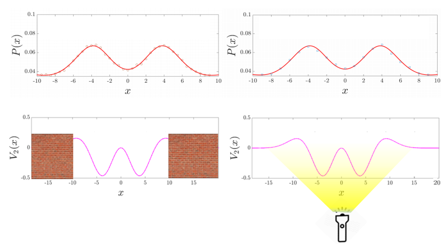
Figure 2: In an open system, stretching from ${-\infty}$ to ${\infty}$, the potential ${V(x)=[(x/5)^{4}-2(x/5)^{2}]\exp[-(x/5)^{2}]}$ is weakly binding, like the one seen in Fig. 1c. There are two ways by which one can obtain the Boltzmann distribution in a system with such a potential. Left bottom corner: we place the system within hard walls at ${\pm 10}$, and since the system has a finite size, it has to eventually relax to equilibrium. Upper left corner: we see the simulated position distribution of the particles (blue circles), where the normalization is obtained by dividing the histogram of the positions by the number of particles and a bin-size. The theoretical red curve corresponds to Eq. (2). Right bottom corner: when we remove the hard walls, particles escape freely to infinity. This case is very different from the previous one as here the system size is infinite. However, here we track only the section of ${-10<x<10}$, and the particles which are found there at time ${t}$. Upper right corner: The simulated position distribution of the particles, normalized only with respect to the particles that are found within the “illuminated” region of ${x\in[-10,10]}$ (blue squares) at time ${t=10000}$, versus the same theoretical red curve as above. As predicted by our previous results in Ref. Aghion, Kessler, and Barkai [2019], the upper two pictures are practically indistinguishable, despite describing very different physical scenarios. Our goal in this paper is to investigate in depth the dynamics of the latter scenario.

The structure of the manuscript is as follows: We first discuss in Sec. II some preliminary matters, presenting a brief recap of equilibrium statistical mechanics for binding potentials, where the partition function is normalizable, together with a description of the particular examples of asymptotically flat potentials we use for our simulations. In Sec. III we define the non-normalizable Boltzmann state. In Sec. IV, we discuss the entropy maximization principle. In Sec. V, we provide the derivation of the leading-order time-dependent shape of the particle density and obtain higher-order correction terms. In Sec. VI, we discuss time and ensemble averages, and in Sec. VII we discuss the fluctuations of the time average and infinite ergodic theory. In Sec. VIII, we study the virial theorem. In Sec. IX, we show that the non-normalizable Boltzmann state exists in any dimension ${d\geq 1}$, and extend our analysis of the ratio between time and ensemble averages of integrable observables, to any dimension. A summary of our main results is found in Sec. X. The discussion is found in Sec. XI.

II Preliminaries

II.1 A recap of statistical mechanics

Before treating weakly binding potentials, we first recall the standard treatment of the case where $V(x)$ is increasing with distance in such a way that the partition function is finite, e.g., $V(x)=x^{2}$ (a binding potential, Fig. 1.a). According to the basic laws of statistical physics, the system is ergodic (we assume that $V(x)$ does not divide the system into compartments). Let ${\cal O}[x(t)]$ be a physical observable. Then, in the long-time limit,

$$\overline{{\cal O}[x(t)]}\rightarrow\langle{\cal O}(x)\rangle.$$ (4)

Here, the overline denotes a time-average $\overline{{\cal O}[x(t)]}=\frac{1}{t}{\int_{0}^{t}{\cal O}[x(t^{\prime})]{\rm d}t^{\prime}}$, and the brackets an ensemble-average. The fact that the time-average, which is what is measured in many experiments, converges to the corresponding ensemble-average (in the long-time limit), is very useful for the theoretician, who usually considers the latter;

$$\langle{\cal O}(x)\rangle={\int_{0}^{\infty}{\cal O}(x)\exp[-V(x)/k_{B}T]{\rm d}x\over Z}.$$ (5)

It should be noted that some observables, such as $\mathcal{O}(x)=\exp[V(x)/T]$, are not integrable with respect to the Boltzmann distribution, however these are mostly not the main focus of physicists.

Statistical mechanics is related to thermodynamics in many textbooks. In particular, the Helmholtz free energy is

$${\cal F}=\langle V\rangle-TS,$$ (6)

where we omitted the thermal kinetic energy term without any loss of generality. The entropy is

$$S(t)=-k_{B}\int_{0}^{\infty}P_{t}(x)\ln[P_{t}(x)]{\rm d}x,$$ (7)

where $P_{t}(x){\rm d}x$ is the probability of finding the particle at time $t$ in the interval $(x,x+{\rm d}x)$. In equilibrium, we take the long-time limit, and for generic initial conditions we have

$$\lim_{t\to\infty}P_{t}(x)=P_{{\rm eq}}(x),$$ (8)

so, in this limit,

$${\cal F}=-k_{B}T\ln Z,$$ (9)

and

$$P_{{\rm eq}}(x)={e^{-V(x)/k_{b}T}\over e^{-{\cal F}/k_{b}T}}.$$ (10)

The Boltzmann factor appearing in the numerator is the essence of the canonical ensemble, while in the denominator we have the relation to thermodynamics. The goal of this manuscript is to consider the case where $S$ is increasing with time, as opposed to saturating to a limit, but still all this structure remains intact when the appropriate modifications are made, namely we must use the tool of non-normalizable Boltzmann-Gibbs statistics Dechant et al. [2011]; Aghion, Kessler, and Barkai [2019]; Wang, Deng, and Chen [2019]. This idea, which is discussed at length below, harnesses the tools of infinite-ergodic theory, which has been well established as a mathematical theory for several decades, and was discovered in recent years also in physical systems, e.g., Darling and Kac [1957]; Aaronson [1997]; Zweimüller [2009]; Thaler [2001]; Akimoto and Miyaguchi [2010]; Korabel and Barkai [2012]; Klages [2013]; Akimoto, Shinkai, and Aizawa [2015]; Meyer and Kantz [2017]; Leibovich and Barkai [2019]; Akimoto, Barkai, and Radons [2019]; Zhou, Xu, and Deng [2019]; Sato and Klages [2019]; Radice et al. [2020]. Note that infinite, namely non-normalizable, densities serve two main goals; the first is for computation of large deviations and rare-event statistics of fat-tailed stochastic systems, and the second is in the context of ergodic theory. In that regard, one should distinguish between infinite invariant and infinite covariant densities, the latter are not discussed here (see e.g., Refs. Kessler and Barkai [2010]; Lutz and Renzoni [2013]; Rebenshtok et al. [2014a, b]; Holz, Dechant, and Lutz [2015]; Aghion, Kessler, and Barkai [2017]; Wang et al. [2019]; Vezzani, Barkai, and Burioni [2019]).

II.2 Asymptotically flat potentials

As mentioned above, in this work we treat the class of potentials where ${V(x)\rightarrow 0}$ at ${x\rightarrow\infty}$, and the drop rate is at least as fast as ${1/x}$. In this case ${V(x)}$ belongs to the larger class of potentials which are weakly binding. Our leading-order results below apply to any such asymptotically flat potential; however, some of our calculations of higher-order correction terms below are obtained only for potentials that fall-off faster than ${1/x^{2}}$. Furthermore, we distinguish between two situations: the one-sided case, where $V(x)=\infty$ when $x\leq 0$, and the double-sided system, where, to simplify explanations, we assume that the system is symmetric, and so ${V(x)\rightarrow 0}$ also when ${x\rightarrow-\infty}$ (but our results can be trivially extended also to the non-symmetric case). The first situation can be realized experimentally, for example, when the particles are diffusing in three dimensions in a heat bath, above a flat surface, and their interaction with that surface is given by ${V(x)}$, where ${x}$ is their height (see e.g., Pavani et al. [2009]; Chechkin et al. [2012]; Metzler et al. [2014]; Campagnola et al. [2015]; Krapf et al. [2016]; Wang, Wu, and Schwartz [2017]). Here, the potential is infinite when ${x}$ is zero, since the surface is impenetrable. The second case, corresponds e.g., to a scenario where the particles diffuse in a liquid while being loosely held by optical tweezers. The intensity of such an optical trap drops with the distance from the potential well, often like an inverted Gaussian Ashkin et al. [1986]; Grier and Roichman [2006]; Drobczynski and Ślezak [2015].

In our simulations, we mostly used the following two examples: the one-sided Lennard-Jones type potential (which depends only on the height coordinate, $x$, in the scenario of three dimensional diffusion above a hard-surface):

$$V(x)=\left\{\begin{array}[]{c c}\infty&x\leq 0\\ V_{0}\left[\left({a\over x}\right)^{12}-\left({b\over x}\right)^{6}\right]&x>0\end{array}\right.,$$ (11)

where $V_{0}$, $a$ and $b$ are positive constants, and the symmetric potential (which can be realized using optical tweezers e.g., Grier and Roichman [2006]; Drobczynski and Ślezak [2015]):

$$V(x)=\left[(x/5)^{4}-(x/5)^{2}\right]e^{-(x/5)^{2}}.$$ (12)

In both cases, there is no thermal equilibrium in the usual sense. Famously, this “problem” with asymptotically flat potentials was pointed out by Fermi already in $1924$ Fermi [1924]. Physically, when $x$ is large, the deterministic force is negligible and then the particles are diffusing in the bulk. Our discussion below is not limited to a specific form of the potential field, provided that it is eventually flat, but the key assumption is that the fluctuation-dissipation relation applies, namely the Einstein relation is valid. This fact, as we show, allows for modified thermal concepts to emerge, even though $Z=\infty$. Note that unless specified explicitly, below we present our derivations mostly for the one-sided potentials, just for simplicity of writing.

II.3 Limitations of the standard treatment of the non-normalizability of the partition function, and the alternative

The standard response to the “problem” of the divergence of the Boltzmann factor, for any type of potential, is to introduce a finite size to the system, $L$, and since then the limits of the integral in Eq. (3) will stretch only up to this limit, it is guaranteed to have a finite value. In this case, the system will always approach equilibrium in the long-time limit. On the bottom-left panel of Fig. 2, we see an example of a system enclosed between two walls, with a potential that, without the walls (namely, if the system had stretched from ${-\infty}$ to ${\infty}$), would have been weakly binding. On the top-left panel of the figure, we see the corresponding Boltzmann distribution of the particles. But in this work, we do not wish to impose this constraint. One reason is simply that many experimental settings do not have truly hard walls or confining potentials e.g., when using optical traps (see for example, Grier and Roichman [2006]; Drobczynski and Ślezak [2015]). The second reason is that even when the systems is confined by its boundaries, very often particle tracking experiments are not long enough for the particles to encounter them.

The results of our previous work, Ref. Aghion, Kessler, and Barkai [2019], imply that we can take a very different physical approach, but still retain the exact same shape of $P_{t}(x)$ at long times, obtained in the hard-wall scenario. In this second approach, we focus our range of observation to a single slice of space, and normalize the probability distribution only with respect to the number of particles that are present in this region at time ${t}$ (namely, by discarding the particles which are found outside of this region). Note, that this situation is common in single-particle-tracking experiments, where the microscope in use has a finite field of view, hence this approach is essentially similar to “looking under the lamp”. The result of a simulation of this is shown in the right side of Fig. 2, to be compared with the wall scenario on the left. The measured concentration of the remaining particles is identical (up to statistical fluctuations) to that of the equilibrium state of the “walled” system, even though the distributions come from two different physical setups. As we shall see in the following, the dynamics by which the two final distributions are attained are extremely different. The “walled” system converges exponentially in time (with the time diverging as $L\to\infty$), whereas the alternative converges as a power-law.

III The non-normalized Boltzmann-Gibbs state

In this section, we review the derivation of the long-time limit of the distribution function to leading-order. We then analyze its thermodynamic implications. We start from the Fokker-Planck equation description of the diffusion process controlled by the Langevin Eq. (1), which specifies the dynamics of the concentration of particles, or equivalently the probability density function $P_{t}(x)$,

$${\partial P_{t}(x)\over\partial t}=D\left[{\partial^{2}\over\partial x^{2}}+{\partial\over\partial x}{V^{\prime}(x)\over k_{B}T}\right]P_{t}(x).$$ (13)

We treat this equation in the long-time limit. If we set the left-hand side to zero, namely we search for a time-independent solution, which we call ${\cal I}(x)$, we have

$$0=\left[{\partial^{2}\over\partial x^{2}}+{\partial\over\partial x}{V^{\prime}(x)\over k_{B}}T\right]{\cal I}(x),$$ (14)

and hence one appealing option reads

$${\cal I}(x)=\mbox{Const}\exp\left[-V(x)/k_{B}T\right].$$ (15)

However, this solution does not satisfy the boundary condition $\lim_{x\to\infty}P_{t}(x)=0$ (unless $\mbox{Const}=0$) and is clearly non-normalizable when ${V(x)}$ is asymptotically flat at large distances. This is certainly not a possibility as the particles are neither created nor annihilated, so the normalization is conserved $\int_{0}^{\infty}P_{t}(x){\rm d}x=1$ for any $t\geq 0$. In-fact, mathematically as we will show below, the non-normalized solution ${\cal I}(x)$ is an infinite-invariant density Aaronson [1997], as opposed to a probability density.

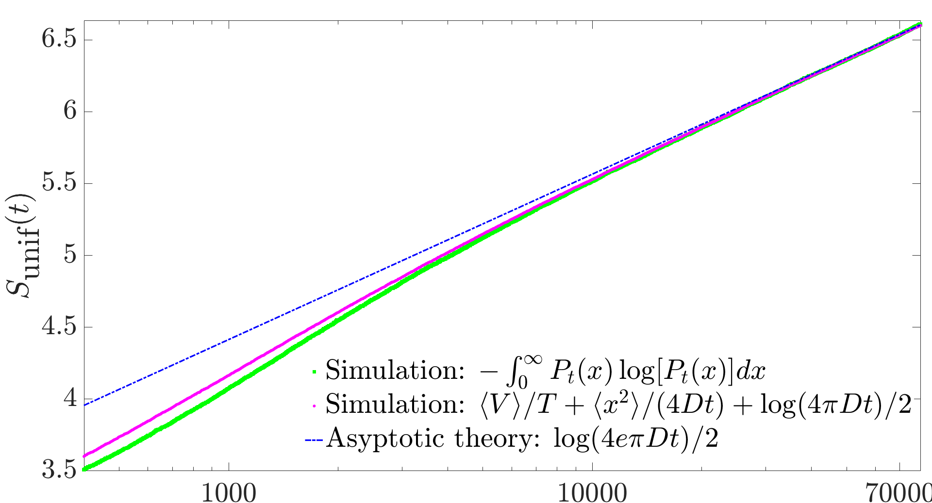
Figure 3: (color online) The Gibbs entropy, $S(t)=-\int_{0}^{\infty}P_{t}(x)\log{[P_{t}(x)]}\textrm{d}x$, obtained from simulation results of the overdamped Langevin Eq. (1), and the symmetric potential Eq. (12), for $10^{5}$ particles, at $k_{B}T=0.2$ (green squares). The purple circles corresponds to Eq. (21) (but with ${\pi\rightarrow 4\pi}$, since the potential is symmetric), where all the observables are measure from the simulation. Here, one should note that additional correction terms of order ${1/\sqrt{t}}$ might exist, due to contribution from correction terms to the leading-order behavior of ${P_{t}(x)}$, discussed in Sec. V. Such correction terms will decay in time as fast as ${\langle V\rangle}$. The blue line corresponds to the asymptotic theory, Eq. (22) (with ${\pi\rightarrow 4\pi}$), which becomes exact when $t\rightarrow\infty$.

Since ${\mathcal{I}(x)}$ is non-normalized, we search for a more complete solution in the form of

$$P_{t}(x)\sim{Ae^{-{V(x)\over k_{B}T}}\over t^{\alpha}}$$ (16)

with $\alpha>0$. The logic behind this ansatz is that, instead of Eq. (15) which is obtained from Eq. (14) where the left-hand side is exactly zero, we now look for a time-dependent solution to Eq. (13), where the contribution from the left-hand side is non-zero, yet small. This long-time behavior, when inserted into the Fokker-Planck equation, is a solution to leading-order, with correction terms of order $\partial_{t}t^{-\alpha}\propto t^{-(1+\alpha)}$ which are smaller by a factor of $1/t$ than the leading $t^{-\alpha}$ term. Physically, we can expect this solution to be valid only for $x\ll l(t)$, where $l(t)=\sqrt{4Dt}$ is the diffusion length-scale of the problem. In the range $x\gg 1$, on the other hand, we know that the force is negligible. Hence, in that case,

$$P_{t}(x)\simeq{1\over\sqrt{\pi Dt}}\exp[-{x^{2}\over 4Dt}].$$ (17)

Matching Eqs. (16,17) in the overlap region $1\ll x\ll l(t)$, we find $\alpha=1/2$ and $A=1/\sqrt{\pi D}$. A uniform approximation then reads

$$P_{t}(x)\simeq{1\over\sqrt{\pi Dt}}e^{-{V(x)\over k_{B}T}}e^{-{x^{2}\over 4Dt}},$$ (18)

where we set $V(\infty)=0$. This scaling solution is valid at long times for all $x$. For a process with a potential of the form in Eq. (12), where the particle is allowed to cross also to ${x<0}$, the factor ${\sqrt{\pi Dt}\rightarrow 2\sqrt{\pi Dt}}$, and similarly ${A\rightarrow A/2}$ in Eq. (16). In Sec. V we derive this solution for any potential which decays faster than ${1/x^{2}}$ at large distances, using an eigenfunction expansion method that employs the continuous spectrum of the Fokker-Planck operator. This method also yields correction terms that vanish faster than ${1/\sqrt{t}}$. We leave the equivalent derivation for the case of potentials that fall off like ${1/|x|^{\zeta}}$, where ${1<\zeta\leq 2}$, out of this manuscript, since here all the results associated with the leading order behavior in time are similar to the ${\zeta>2}$ case, but the correction terms are different.

Importantly, to obtain Eq. (18), we have assumed that the particles are initially localized, say on $x_{0}$ or within an interval $(0,x_{0})$, or more correctly the initial density has at least an exponential cutoff. The scale $x_{0}$ does not alter the long-time solution (to leading-order approximation, see Sec. V), and since the solution forgets its initial conditions, we introduce a thermodynamic notation

$$P_{t}(x)\propto e^{-\beta V(x)-\xi x^{2}}$$ (19)

with $\beta=1/k_{B}T$ and $\xi=1/4Dt$.

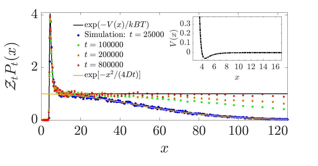
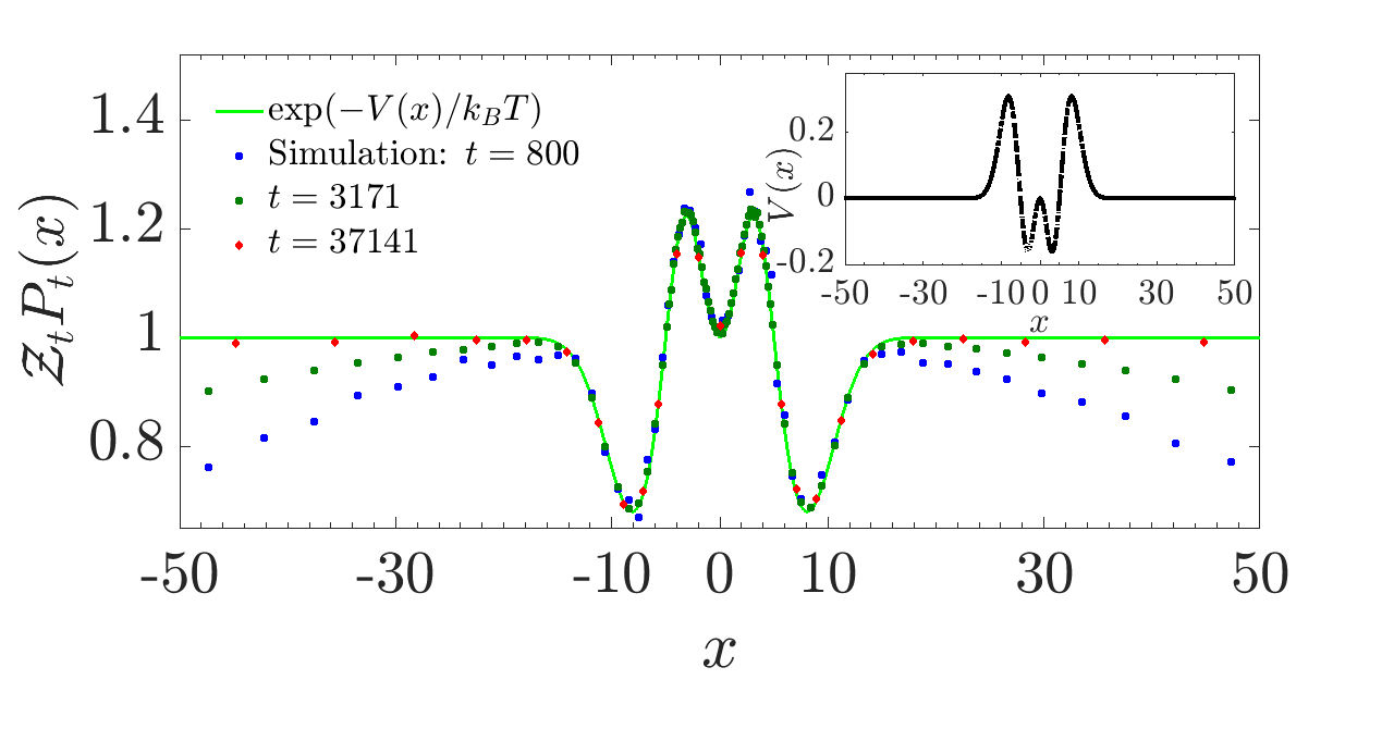
Figure 4: (Color online) Upper panel: The non-normalizable Boltzmann state Eq. (24), corresponding to the Lennard-Jones potential, Eq. (11); Theory in black line, simulation results for ${\mathcal{Z}_{t}P_{t}(x)}$, at various increasing times ${t}$, where ${\mathcal{Z}_{t}=\sqrt{\pi Dt}}$ (${k_{B}T=~{}0.0436}$, ${\gamma=1}$), appear in colored symbols. The inset shows the potential, where ${U_{0}=1000}$ and ${(a,b)=(1,2)}$. At finite times one can see deviations from the asymptotic Boltzmann state, which vanish as ${t}$ increases. As seen by the yellow line (at e.g., ${t=2500}$), at large ${x}$, ${P_{t}(x)}$ is Gaussian (since the attractive force is zero). Lower panel: The non-normalizable Boltzmann state corresponding to the two-sided potential Eq. (12), with ${(k_{B}T,\gamma)=(0.8,1)}$ (green curve). Here ${\mathcal{Z}_{t}\rightarrow{2\mathcal{Z}_{t}}}$. Simulation results in colored symbols (and the inset shows the potential).

We now consider the entropy of the system. Using the uniform approximation, Eq. (18), we find

$$S_{\mbox{unif}}(t)=k_{B}\int_{0}^{\infty}{\rm d}xP_{t}(x)\left[\ln\sqrt{\pi Dt}+\beta V(x)+\xi x^{2}\right].$$ (20)

This yields

$$S_{\mbox{unif}}(t)={\langle V\rangle\over T}+k_{B}\xi\langle x^{2}\rangle-{\cal{\tilde{F}}}/T,$$ (21)

where the averages are with respect to Eq. (18). The average energy $\langle V\rangle$ and $\beta$ are thermodynamic pairs, and at least suggestively the same is true for $\langle x^{2}\rangle$ and $\xi$. Later, we will make this analogy to equilibrium statistical mechanics more precise, using an entropy maximization formalism. Here, the free energy is ${\cal\tilde{F}}=-(k_{B}T/2)\ln(\pi/4\xi)$. It stems from the first term in Eq. (20), which in the usual setting gives the connection between the Helmholtz free energy and the partition function. We now see that, for a fixed observation time and ${D}$; Eq. (21) means that $1/T=(\partial S_{\mbox{unif}}/\partial\langle V\rangle)$, in agreement with standard thermodynamics. To leading order, using the fact that the mean-squared displacement is behaving diffusively at long times, namely $k_{B}\langle x^{2}\rangle/4Dt=k_{B}/2$, we have

$$S_{\mbox{unif}}(t)\sim{k_{B}\over 2}-{\cal{\tilde{F}}}/T={k_{B}\over 2}\ln(\pi eDt).$$ (22)

In this limit, the entropy is insensitive to the potential, since the average potential energy approaches zero at increasing times. This occurs simply because the particles increasingly explore the large ${x}$ region where the potential is flat (zero). Below, we study the average potential energy in detail, but for now it is only important to realize that entropy times $T$ is far larger. Eq. (22) shows that the entropy is increasing with time, which is to be expected, since the packet of particles is spreading out to the medium. Fig. 3 shows the entropy versus time, obtained from simulation results using the two-sided potential, Eq. (12) (green squares), and the corresponding measurement based on Eq. (21) (purple circles). But in the latter, since the potential is symmetric, ${S_{\mbox{unif}}(t)\sim\frac{k_{B}}{2}\ln{(4e\pi Dt)}}$ (the reason is that at the tails, the density is now proportional to ${\exp[-x^{2}/(4Dt)]/\sqrt{4\pi Dt}}$). It also shows the asymptotic logarithmic growth at long times (blue line), based on Eq. (22), but with ${\pi\rightarrow 4\pi}$. The figure shows that Eq. (21) is a good approximation, but note that additional correction terms of order ${1/\sqrt{t}}$ might exist, due to contribution from correction terms to the leading-order behavior of ${P_{t}(x)}$, discussed in Sec. V, which will decay in time as fast as ${\langle V\rangle}$. Even in this case, the asymptotic logarithmic growth at long times, seen in Eq. (22), will remain unchanged.

We are now ready to define the non-normalized Boltzmann density more precisely. We define the time dependent function

$$\mathcal{Z}_{t}=\exp(-{\cal\tilde{F}}/k_{B}T),$$ (23)

hence in our case $\mathcal{Z}_{t}=\sqrt{\pi Dt}$ (or ${\sqrt{4\pi Dt}}$ for two-sided potentials). Inserting ${\mathcal{Z}_{t}}$ into Eq. (18), we find

$$\lim_{t\to\infty}\mathcal{Z}_{t}P_{t}(x)=\exp[-V(x)/k_{B}T].$$ (24)

Here we used $\lim_{t\to\infty}\exp[-x^{2}/4Dt]=1$ for any finite $x$, though in a finite-time experiment, this identity will be valid for $x\ll l(t)=\sqrt{4Dt}$.

At least in principle, with a measurement of the entropy in the long-time limit, which is possible with an ensemble of particles, and using Eqs. (22,23), we can determine $\mathcal{Z}_{t}$. And with that information, we can verify Eq. (24). Note that, clearly, if we know $D$ up front, we can find $\mathcal{Z}_{t}$ without measuring entropy at all, but one point of our work is to claim that the thermodynamic formalism may have a more general validity, which is a question worthy of further study. Since $\mathcal{Z}_{t}$ is increasing with time, then when it is multiplied by the normalized density $P_{t}(x)$, this leads to a non-normalizable Boltzmann factor, when $t$ becomes large. Again, mathematically, the non-normalized Boltzmann factor is the infinite-invariant density of the system Aaronson [1997]; Aghion, Kessler, and Barkai [2019]. Of course Eq. (24) holds also for the case when $\mathcal{Z}_{t}$ eventually approaches a constant, namely for finite size systems. Fig. 4, shows simulation results for ${\mathcal{Z}_{t}P_{t}(x)}$, corresponding to the potentials in Eq. (11) (top figure), and Eq. (12) (bottom). At increasing times, the scaled distributions approach the non-normalizable Boltzmann state, Eq. (24), while the finite-time Gaussian tails where ${x\sim\sqrt{t}}$, are pushed increasingly outward. The insets show the potentials. Note that we obtain the correction terms to the leading behavior of ${P_{t}(x)}$ in Sec. V, but for now we leave the rest of the discussion about the corrections to the mean energy and entropy out of the scope of this manuscript. The benefit of that discussion is in the rigorous derivation of the shape of ${P_{t}(x)}$ and the effect of the initial condition, which is shown to be negligible (namely it does not alter Eq. (24)).

Using Eq. (24), one can determine the shape of the potential field in the system from the position density of the particles. We do not, however, address the question of whether this yields the mechanical or electrostatic force, or an effective force, as clearly the potential of the mean force might itself be temperature-dependent.

IV Entropy extremum principle

The structure of the theory suggests that a more general principle is at work. The entropy extremum principle is a natural choice, with the imposition of three added constraints. These are: the normalization condition, a finite mean energy condition (this allows us to treat fluctuations of energy in the canonical ensemble, unlike the microcanonical ensemble, where the energy surface is fixed), and the special feature of our system, which is that the mean-squared displacement is diffusive, $\langle x^{2}\rangle\sim 2Dt$. This latter constraint is the new ingredient of the theory and this introduces the time dependency.

We define a functional of the density $P_{t}(x)$ at some fixed large $t$

$${\cal S}[P_{t}(x)]= -k_{B}\int_{0}^{\infty}P_{t}(x)\ln P_{t}(x){\rm d}x$$

$$-\beta k_{B}\left(\int_{0}^{\infty}V(x)P_{t}(x){\rm d}x-\langle V\rangle\right)$$

$$-\lambda k_{B}\left(\int_{0}^{\infty}P_{t}(x){\rm d}x-1\right)$$

$$-\xi k_{b}\left(\int_{0}^{\infty}x^{2}P_{t}(x){\rm d}x-2Dt\right).$$ (25)

Here $\beta,\lambda$ and $\xi$ are Lagrange multipliers. The first term is the entropy, which in the absence of the constraints implies that all micro-states are equally probable. If we set $\xi=0$, and find the extremum, we get the usual Boltzmann-Gibbs theory, however that can be valid only if the potential is binding, which is not the case under study here. Taking the functional derivative, we get

$$P_{t}(x)=N\exp\left(-\beta V(x)-\xi x^{2}\right),$$ (26)

where $N$ is the normalization constant. The constraints are

$$N\int_{0}^{\infty}\exp\left[-\beta V(x)-\xi x^{2}\right]{\rm d}x=1,$$

$$N\int_{0}^{\infty}x^{2}\exp\left[-\beta V(x)-\xi x^{2}\right]{\rm d}x=2Dt,\quad\mbox{and}$$

$$N\int_{0}^{\infty}V(x)\exp\left[-\beta V(x)-\xi x^{2}\right]{\rm d}x=\langle V(x)\rangle.$$ (27)

These conditions are satisfied if $\xi$ is small and $V(x)$ is asymptotically flat. To see this, we use $\xi x^{2}=y^{2}$, so we can rewrite the first two integrals as:

$${N\over\sqrt{\xi}}\int_{0}^{\infty}\exp\left[-\beta V(y/\sqrt{\xi})-y^{2}\right]{\rm d}y=1$$ (28)

and

$${N\over\sqrt{\xi}^{3}}\int_{0}^{\infty}y^{2}\exp\left[-\beta V(y/\sqrt{\xi})-y^{2}\right]{\rm d}y=2Dt,$$ (29)

and since $\lim_{\xi\to 0}V(y/\sqrt{\xi})=0$ we may ignore the potential field in this limit. Solving the Gaussian integrals, we find

$$\xi={1\over 4Dt},\ \ \ \ N={1\over\sqrt{\pi Dt}}.$$ (30)

Notice that in Eqs. (28,29), we are averaging over observables which are non-integrable with respect to the Boltzmann infinite density, i.e. $x^{0},x^{2}$ (or $y^{0},y^{2}$). For the last constraint we use the small parameter $\xi$ to approximate $V(x)\exp[-\beta V(x)-\xi x^{2}]\to V(x)\exp[-\beta V(x)]$, and since in any reasonable range where the potential is finite, $\exp[-\xi x^{2}]$ is equal to $1$, we get $\langle V\rangle=N\int_{0}^{\infty}V(x)\exp[-\beta V(x)]{\rm d}x.$ To summarize, we find that the extremum principle gives

$$P_{t}(x)\simeq{\exp\left[-\beta V(x)-x^{2}/4Dt\right]\over\sqrt{\pi Dt}}.$$ (31)

This is the same as the uniform approximation Eq. (18), which was proven valid for a specific stochastic model, i.e. the overdamped Langevin equation. However, the extremum principle suggests that the existence of the non-normalized Boltzmann density is of more general validity, even outside of this particular context. Finally, one could claim that since thermodynamics is a theory which does not depend explicitly on time $t$, we cannot identify $\beta$ with the inverse of the temperature. However, at least within our Langevin model, the Einstein relation and our analytical results give both the physical and the mathematical motivation to make this relation.

V Eigenfunction expansion, and corrections to the uniform approximation

We have obtained the leading-order behavior of ${P_{t}(x)}$ at long times for asymptotically flat potentials from two different directions, first by using physically inspired guesses for the small and large $x$ regimes and then matching, and secondly via entropy maximization. Here, we re-derive our result a third time, but importantly, now we use an eigenfunction expansion, so as to allow access to the leading-order corrections. In particular, we focus on potentials that fall off faster than ${1/x^{2}}$ at large ${x}$. The spectrum of the Fokker-Planck operator is continuous since the system is diffusive in the bulk. For convenience, we consider the case that there is a reflecting wall at $x=0$, giving rise to a no-flux boundary condition, $P_{t}^{\prime}(0)=0$. The final answer works as well for the case that the potential diverges to $+\infty$ as $x\to 0$ from above, so that again the particles are restricted to $x>0$. For a ${\delta}$-function initial distribution, centered around some positive ${x_{0}}$, we show that the initial condition does not affect the asymptotic shape to leading order in time, and we obtain the correction to the leading-order term where it first makes its appearance. Note that the eigenfunction expansion in the case of a two-sided potential follows along the same lines, but given the details of the setup one may need to examine both symmetric and non-symmetric solutions for the eigenmodes.

Starting from the Fokker-Planck equation,

$${\partial_{t}P_{t}(x)=\hat{L}_{\textit{FP}}P_{t}(x),}$$ (32)

where ${\hat{L}_{\textit{FP}}=D[\partial^{2}_{x}+\partial_{x}U^{\prime}(x)]}$ is the Fokker-Planck operator and ${U(x)=\frac{V(x)}{k_{B}T}}$, using the unitary transformation Dechant et al. [2011] ${\hat{\mathcal{H}}=e^{U(x)/2}\hat{L}_{FP}e^{-U(x)/2}}$, $\Psi(x,t)=e^{U(x)/2}P_{t}(x)$, we write the following Schrödinger-like equation

$${\hat{\mathcal{H}}\Psi(x)=-\lambda\Psi(x).}$$ (33)

For technical reasons, we imagine an infinite effective-potential wall at large $x=L$, so that the spectrum is discrete. As the eigenvalues $\lambda$ are positive definite ($\lambda=0$ is not in the spectrum as it is not normalizable in the $L\to\infty$ limit, and hence the system does not reach equilibrium Dechant et al. [2011]), we write $\lambda\equiv Dk^{2}$, for some discrete set of $k$’s. We will eventually take the $L\to\infty$ limit, before we take the large $t$ limit. Then,

$${P_{t}(x)=e^{-U(x)/2+U(x_{0})/2}\sum_{\{k\}}N_{k}^{2}\Psi_{k}(x_{0})\Psi_{k}(x)e^{-Dk^{2}t}.}$$ (34)

It will prove convenient to set the normalization of $\Psi_{k}(x)$ via the condition $\Psi_{k}(0)=e^{-U(0)/2}$, so we have to incorporate an explicit normalization factor $N_{k}^{2}$. Thus, Eq. (33) translates to

$${\frac{\partial^{2}}{\partial x^{2}}\Psi_{k}(x)+\frac{U^{\prime\prime}(x)}{2}\Psi_{k}(x)-\frac{U^{\prime 2}(x)}{4}\Psi_{k}(x)=-k^{2}\Psi_{k}(x).}$$ (35)

with boundary conditions

$$\Psi_{k}(0)=e^{-U(0)/2},\qquad\Psi_{k}^{\prime}(0)=-\frac{U^{\prime}(0)}{2}e^{-U(0)/2}.$$ (36)

The long-time limit is clearly dominated by the small-$k$ modes, so we need to consider only them. We need to treat two regimes separately, first the range ${x\ll 1/{k}}$, where the right-hand side of Eq. (35) is always small, (denoted region I), and second, for ${x\gg 1}$ (region III). We match the two asymptotic limits in the overlap region ${1\ll x\ll 1/k}$ (region II).

In Region I, the term $-k^{2}\Psi_{k}(x)$ is negligible due to the smallness of $k$. To leading order, then, we have the homogeneous equation,

$${\frac{\partial^{2}}{\partial x^{2}}\Psi_{k}(x)+\frac{U^{\prime\prime}(x)}{2}\Psi_{k}(x)-\frac{U^{\prime 2}(x)}{4}\Psi_{k}(x)=0,}$$ (37)

with the solution (satisfying the no-flux boundary conditions Eq. (36) at $x=0$) ${\Psi_{h}(x)=e^{-U(x)/2},}$ corresponding to the non-normalizable zero-mode. To next order, we write ${\Psi_{k}(x)\sim\Psi_{h}(x)-k^{2}e^{-U(x)/2}f(x).}$ Plugging this ansatz into Eq. (35), we get

$${-U^{\prime}(x)f^{\prime}(x)+f^{\prime\prime}(x)=1.}$$ (38)

The boundary conditions, Eq. (36), which apply for any ${k}$, translate to ${f(0)=f^{\prime}(0)=0}$ and so a simple calculation yields

$${f(x)=\int_{0}^{x}e^{U(x^{\prime})}\int_{0}^{x^{\prime}}e^{-U(x^{\prime\prime})}\textrm{d}x^{\prime\prime}\textrm{d}x^{\prime}.}$$ (39)

The behavior of $f(x)$ for large $x$ can be analyzed as follows. Define $f_{1}(x)\equiv\int_{0}^{x}e^{-U(x^{\prime})}\textrm{d}x$. Then, for large $x$,

$$f_{1}(x) =\int_{0}^{x}(e^{-U(x^{\prime})}-1+1)\textrm{d}x$$

$$=x+\int_{0}^{\infty}(e^{-U(x^{\prime})}-1)\textrm{d}x-\int_{x}^{\infty}(e^{-U(x^{\prime})}-1)\textrm{d}x$$

$$\approx x+\ell_{0}$$ (40)

where we have defined the length $\ell_{0}\equiv\int_{0}^{\infty}(e^{-U(x^{\prime})}-1)\textrm{d}x$ (note that ${\ell_{0}}$ is related to the second virial coefficient, see Sec. VIII). Now, for large $x$,

$$f(x) =\int_{0}^{x}\left[e^{U(x^{\prime})}f_{1}(x)-x-\ell_{0}+x+\ell_{0}\right]\textrm{d}x$$

$$=\frac{x^{2}}{2}+\ell_{0}x+\int_{0}^{\infty}\left[e^{U(x^{\prime})}f_{1}(x)-x-\ell_{0}\right]\textrm{d}x$$

$$\qquad\qquad{}-\int_{x}^{\infty}\left[e^{U(x^{\prime})}f_{1}(x)-x-\ell_{0}\right]\textrm{d}x$$

$$\approx\frac{x^{2}}{2}+\ell_{0}x+\mathcal{A}$$ (41)

where the constant $\mathcal{A}$ with units of length² is defined as $\mathcal{A}\equiv\int_{0}^{\infty}\left[e^{U(x^{\prime})}f_{1}(x)-x-\ell_{0}\right]\textrm{d}x.$ This behavior of $f$ can be seen to be consistent with the differential equation, Eq. (38). In the matching region II, where ${1\ll x\ll 1/k}$, therefore:

$${\Psi_{match}(x)\approx 1-k^{2}(x^{2}/2+\ell_{0}x+\mathcal{A})}$$ (42)

In region III, since ${x\gg 1}$, the ${U^{\prime\prime}(x)}$ and ${U^{\prime 2}(x)}$ terms are negligible, and therefore, Eq. (35) now reads

$${\frac{\partial^{2}}{\partial x^{2}}\Psi_{k}(x)\sim-k^{2}\Psi_{k}(x),}$$ (43)

whose solution is ${\Psi_{k}(x)\approx A_{k}\cos(kx)+B_{k}\sin(kx)}$. Comparing this solution with Eq. (42) in the matching region, we find that ${A_{k}=1-k^{2}\mathcal{A}}$ and ${B_{k}=-k\ell_{0}}$. We see that, if ${U(x)=0}$, we have ${l_{0}=0}$, and thus ${B_{k}=0}$, namely in the force-free case the ${\sin(kx)}$ term is absent, as it should. We are now in a position to calculate the normalization

$${N_{k}^{2}=\frac{2}{L(A_{k}^{2}+B_{k}^{2})}\approx\frac{2}{L}(1+2\mathcal{A}k^{2}-\ell_{0}^{2}k^{2}).}$$ (44)

It is interesting to note that the presence of the $B_{k}$ term, induced by the presence of $U(x)$, results in a $O(1)$ leftward shift of $\ell_{0}$ in the original pure $\cos$ wave of the free particle case, in additional to the small change in normalization. This has a simple physical interpretation, which we will return to below.

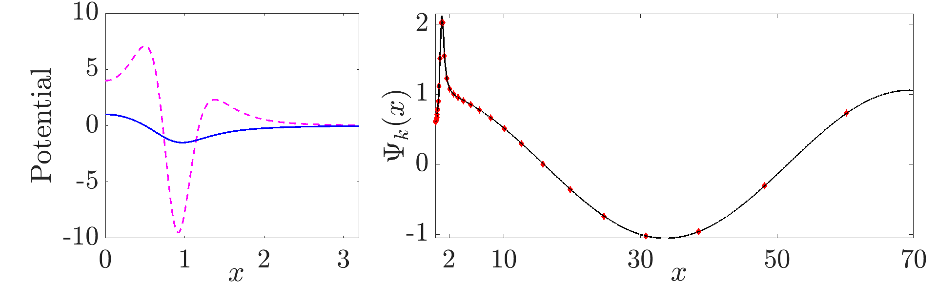
Figure 5: (color online) Left panel: The potential ${U(x)=(1-4x^{2})/(1+x^{6})}$, (blue line), and the effective potential in the Schrödinger Eq. (35): ${=-U^{\prime\prime}(x)/2+U^{\prime 2}(x)/4}$ (magenta dashed line). Right panel: The eigenfunction ${\Psi_{k}(x)}$, Eq. (45) (red diamonds), compared with the exact numerical solution of the Schrödinger Eq. (35) (black line), with the potential ${U(x)=(1-4x^{2})/(1+x^{6})}$ and ${k=0.088}$. At small ${x}$, the eigenfunction reflects the shape of the potential, since it is proportional to ${\exp[-U(x)/2]}$ (region I). At large ${x}$ (region III), the solution is proportional to ${A_{k}\cos(kx)+B_{k}\sin(kx)}$ (see Eq. (43)).

A uniform approximation, for any ${x}$, is seen to be:

$$\Psi_{k}(x) \approx e^{-U(x)/2}\Big{[}\cos(kx)(1-k^{2}(\tilde{f}(x)+\mathcal{A}))$$

$$\qquad\qquad\qquad{}-k\ell_{0}\sin(kx)\Big{]}$$ (45)

where we have defined

$${\tilde{f}(x)\equiv f(x)-x^{2}/2-\ell_{0}x-\mathcal{A}.}$$ (46)

In the left panel of Fig. 5, we show the potential, ${U(x)=(1-4x^{2})/(1+x^{6})}$, and the effective potential in the “quantum” problem, namely: ${-U^{\prime\prime}(x)/2+U^{\prime 2}(x)/4}$. In the right panel, we show that ${\Psi_{k}(x)}$ from Eq. (45) matches the exact numerical solution of the Schrödinger Eq. (35), with the above mentioned potential and ${k=0.088}$.

We are now in a position to take the $L\to\infty$ limit, wherein the sum over $n$ transforms into an integral over $k$, ${\sum_{k}\rightarrow\int\textrm{d}k\frac{L}{\pi}}$.

For finite $x$, and $x_{0}$, then, using Eqs. (34) and (44,45) the long-time density reads

$$P_{t}(x) \approx e^{-U(x)}\int_{0}^{\infty}\frac{2\textrm{d}k}{\pi}[1-k^{2}(f(x)+f(x_{0})-2\mathcal{A}+\ell_{0}^{2})]$$

$$\qquad\qquad\qquad\times e^{-Dk^{2}t}$$

$$=\frac{e^{-U(x)}}{\sqrt{\pi Dt}}\left[1-\frac{1}{2Dt}(f(x)+f(x_{0})-2\mathcal{A}+\ell_{0}^{2})\right]$$ (47)

giving us the zeroth-order time-dependent Boltzmann-Gibbs factor, with a $1/t$ correction that grows quadratically in $x$.

We test this prediction in Fig. 6, where we plot the scaled correction $Dt\left(e^{U(x)}-\sqrt{\pi Dt}P_{t}(x)\right)$ and the prediction from Eq. (47), $\frac{1}{2}e^{-U(x)}(f(x)+f(x_{0})-2\mathcal{A}+\ell_{0}^{2})$, for the case $U(x)=(1-4x^{2})/(1+x^{6})$ with $x_{0}=3$. We see that the numerics is converging to the prediction with increasing $t$, with the size of the correction growing as $x^{2}$.

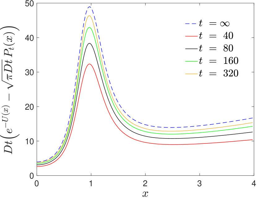
Figure 6: The predicted scaled correction $Dt\left(e^{-U(x)}-\sqrt{\pi Dt}P_{t}(x)\right)$ compared with the prediction from Eq. (47), $\frac{1}{2}e^{-U(x)}(f(x)+f(x_{0})-2\mathcal{A}+\ell_{0}^{2})$, (labelled $t=\infty)$ for the case $U(x)=(1-4x^{2})/(1+x^{6})$ with $x_{0}=3$, for $t=40$, $80$, $160$, $320$. $D=1$. For this potential, $\ell_{0}=2.1719$, $\mathcal{A}=-5.3464$.

To test the dependence on $x_{0}$, we plot in Fig. 7, the predicted correction, and the simulation results at $t=320$ for the same potential, for both $x_{0}=1$ and $x_{0}=3$. The formula is seen to correctly capture the $x_{0}$ dependence, with the correction larger in magnitude for larger $x_{0}$,

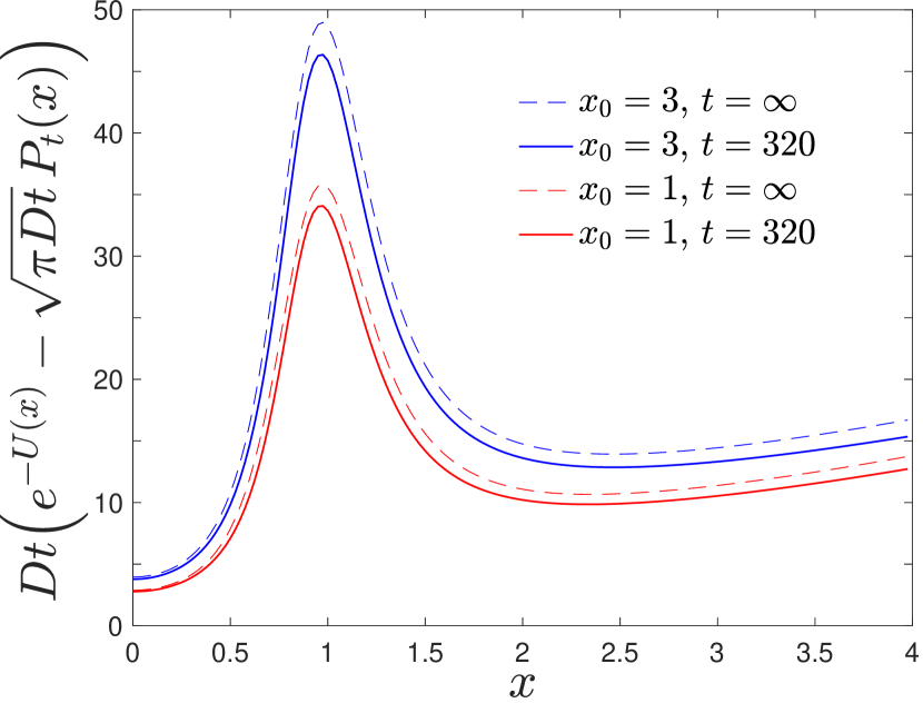
Figure 7: The predicted scaled correction $Dt\left(e^{-U(x)}-\sqrt{\pi Dt}P_{t}(x)\right)$ compared with the prediction from Eq. (47), ${\frac{1}{2}e^{-U(x)}(f(x)+f(x_{0})-2\mathcal{A}+\ell_{0})}$, (labelled $t=\infty)$ for the case $U(x)=(1-4x^{2})/(1+x^{6})$ with $x_{0}=1$ and $x_{0}=3$, for $t=320$. $D=1$, $\ell_{0}=2.1719$, $\mathcal{A}=-5.3464$.

For large $x$, of order $\sqrt{t}$, but $x_{0}$ still $O(1)$, the long-time density is

$$P_{t}(x) \approx\int_{0}^{\infty}\frac{2\textrm{d}k}{\pi}[(1-k^{2}\mathcal{A})\cos(kx)-k\ell_{0}\sin(kx)]$$

$$\qquad\times[1-k^{2}f(x_{0})][1+2k^{2}\mathcal{A}-k^{2}\ell_{0}^{2}]e^{-Dk^{2}t}$$

$$=\frac{e^{-x^{2}/4Dt}}{\sqrt{\pi Dt}}\Bigg{[}1-\frac{2Dt-x^{2}}{4D^{2}t^{2}}(-\mathcal{A}+\ell_{0}^{2}+f(x_{0}))$$

$$\qquad\qquad\qquad\qquad{}-\frac{\ell_{0}x}{2Dt}\Bigg{]}$$ (48)

Thus, it turns out that in this regime, the leading order correction to $P_{t}$ comes from a rightward shift in the Gaussian by an amount $\ell_{0}$, due to the shift in the phase of $\Psi_{k}$ discussed above. Thus, at large distances, the position of the diffusive source is effectively at $x=-\ell_{0}$. As this shift leads to an O($1/\sqrt{t}$) relative change in the solution, if we consider just this leading change, the O($1/t$) terms are negligible, and the solution simplifies to

$${P_{t}(x)\approx\frac{e^{-x^{2}/4Dt}}{\sqrt{\pi Dt}}\Big{[}1-\frac{\ell_{0}x}{2Dt}\Big{]}.}$$ (49)

Note that $\ell_{0}$ may take either positive or negative values hence the sign of the correction term depends on the force field (see Sec. VIII, where we relate $\ell_{0}$ to the virial theorem). This prediction is tested in Fig. 8, where we see very good agreement. In Fig. 9, we check the validity of the $1/t$ relative change via the difference of the simulation to the first order outer solution, Eq. (49), and see that here too the agreement is excellent.

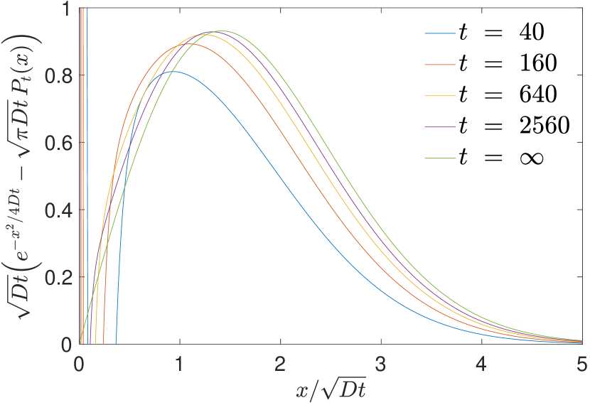
Figure 8: The predicted scaled correction in the outer regime, $x\sim\sqrt{Dt}$, $\sqrt{Dt}(e^{-x^{2}/4Dt}-\sqrt{\pi Dt}P_{t}(x))$ compared with the prediction from Eq. (49), ${\frac{\ell_{0}x}{2}(-\mathcal{A}+\ell_{0}^{2}+f(x_{0}))e^{-x^{2}/4Dt}}$ , (labelled $t=\infty)$ for the case $U(x)=(1-4x^{2})/(1+x^{6})$ with $x_{0}=1$, for $t=40$, $160$, $640$, and $2560$. $D=1$, $\ell_{0}=2.1719$.

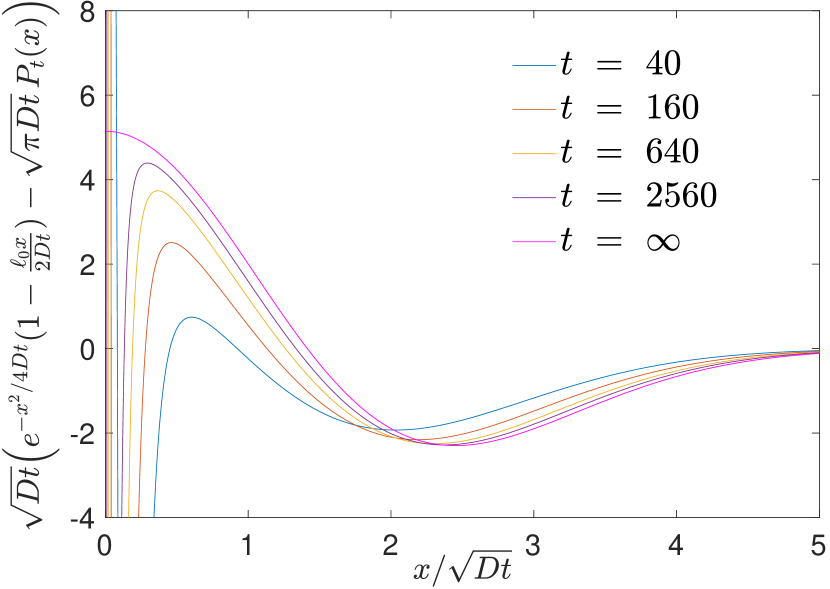
Figure 9: The predicted scaled second order correction in the outer regime, $x\sim\sqrt{Dt}$, $\sqrt{Dt}(e^{-x^{2}/4Dt}\left(1-\frac{\ell_{0}x}{2Dt}\right)-\sqrt{\pi Dt}P_{t}(x))$ compared with the prediction from Eq. (48), ${\frac{2Dt-x^{2}}{4D^{2}t^{2}}e^{-x^{2}/4Dt}}$ , (labelled $t=\infty)$ for the case $U(x)=(1-4x^{2})/(1+x^{6})$ with $x_{0}=1$, for $t=40$, $160$, $640$, and $2560$. $D=1$, $\ell_{0}=2.1719$, $\mathcal{A}=-5.3464$.

More generally, for arbitrary $x$, we have the uniform solution

$$P_{x}(t) \approx\frac{e^{-(x+\ell_{0})^{2}/4Dt}e^{-U(x)}}{\sqrt{\pi Dt}}$$

$$\qquad\times\Bigg{[}1-\frac{2Dt-x^{2}}{4D^{2}t^{2}}(-\mathcal{A}+\ell_{0}^{2}/2+f(x_{0})+\tilde{f}(x))\Bigg{]},$$ (50)

where ${\tilde{f}(x)}$ is defined in Eq. (46). In Sec. VIII.1, we use the next-to leading order behavior of ${P_{t}(x)}$ in order to obtain a correction term to the leading-order, linear behavior of the mean-squared displacement ${\langle x^{2}\rangle}$.

Comment on normalization. We can verify that the solution in Eq. (50) is normalized to unity, in the following way: Integrating ${\exp[-U(x)-x^{2}/(4Dt)]}$, we find that ${\int_{0}^{\infty}e^{-U(x)-\frac{x^{2}}{4Dt}}\textrm{d}x\approx\sqrt{\pi Dt}+\int_{0}^{\infty}(e^{-U(x)}-1)e^{-\frac{x^{2}}{4Dt}}\textrm{d}x,}$ from which, for potentials that fall-off faster than ${1/x^{2}}$ at large ${x}$, in the long-time limit we get ${\int_{0}^{\infty}e^{-U(x)-x^{2}/4Dt}\textrm{d}x\approx\sqrt{\pi Dt}+\ell_{0}}$. So, the first term of $\int_{0}^{\infty}P_{t}(x)\textrm{d}x$ is approximately $1+\ell_{0}/\sqrt{\pi Dt}$. Similarly, the $\ell_{0}x/2Dt$ term in Eq. (49), yields ${-\int_{0}^{\infty}{\ell_{0}xe^{-x^{2}/(4Dt)}\textrm{d}x/[2\sqrt{\pi}(Dt)^{3/2}]}}$. This cancels out the correction to the normalization from the leading term.

VI Time and ensemble-averages

Let us now focus on the limit of long times, where the correction terms to the leading-order behavior of ${P_{t}(x)}$ are negligible with respect to the uniform approximation, Eq. (18). To define the long-time limit of averages, we distinguish between two types of observables: integrable and non-integrable observables, with respect to the non-normalized Boltzmann state. We consider first the indicator function

$${\cal O}[x(t)]=I(x_{1}<x(t)<x_{2}),$$ (51)

where $I(\cdots)=1$ if the condition in the parenthesis is satisfied, and zero otherwise. Along the trajectory ${x(t)}$ of the particle, this observable, ${I(\cdot)}$, switches between values $+1$ and $0$, corresponding to whether the particle is present in the domain $(x_{1},x_{2})$ or not. Here, $x_{1}$ and $x_{2}$ are the experimentalist’s matter of choice.

The ensemble-average of this observable, which in principle can be obtained from a packet of non-interacting particles, at some time $t$ is

$$\langle I(x_{1}<x(t)<x_{2})\rangle =\int_{0}^{\infty}I(x_{1}<x<x_{2})P_{t}(x){\rm d}x$$

$$\sim\int_{x_{1}}^{x_{2}}e^{-\beta V(x)}/\mathcal{Z}_{t}.$$ (52)

This result is valid in the limit of long times, when $x_{1}$ and $x_{2}$ are much smaller than the diffusion length-scale $l(t)=\sqrt{4Dt}$, namely we used the approximation $\exp[-(x_{2})^{2}/4Dt]\simeq 1$. We see that, while the Boltzmann factor $\exp(-\beta V(x))$ is not normalized, it is used to obtain the ensemble averages. In this case the observable is zero at large distances, hence this observable cures the non-integrability of the infinite density. More generally, for observables integrable with respect to the non-normalized Boltzmann factor we have, using Eq. (18)

$$\lim_{t\to\infty}\mathcal{Z}_{t}\langle{\cal O}(x)\rangle=\int_{0}^{\infty}\exp[-\beta V(x)]{\cal O}(x){\rm d}x.$$ (53)

Eqs. (52,53) are valid also for the case when the system reaches a steady state, and then $\mathcal{Z}_{t}$ is the normalizing partition function; in that case Eq. (52) is simply the probability of finding the particle in thermal equilibrium in the interval $(x_{1},x_{2})$.

The time that a particle spends in the domain $(x_{1},x_{2})$ is called the residence time or the occupation time, and it is denoted $t_{x_{1}<x<x_{2}}$. This variable fluctuates from one trajectory to another, however when the system reaches a steady state (i.e. if the potential is binding), the occupation fraction in the long measurement-time limit clearly satisfies $\lim_{t\to\infty}t_{x_{1}<x<x_{2}}/t=\mbox{Prob}(x_{1}<x<x_{2})$ and the latter is obtained from the Boltzmann measure

$$\lim_{t\to\infty}t_{x_{1}<x<x_{2}}/t={\int_{x_{1}}^{x_{2}}e^{-\beta V(x)}{\rm d}x\over Z}.$$ (54)

This result can be obtained also from Birkhoff’s ergodic hypothesis in standard Boltzmann-Gibbs theory.

What is the corresponding behavior for weakly binding potentials where infinite ergodic theory is relevant? The observable $t_{x_{1}<x<x_{2}}/t$ is the finite-time average

$${t_{x_{1}<x<x_{2}}\over t}={\int_{0}^{t}I(x_{1}<x(t)<x_{2}){\rm d}t\over t}.$$ (55)

Let us first consider the ensemble-average of this observable, which is obtained by averaging over an ensemble of paths, each trajectory yielding its own residence time. Here we have

$$\left\langle{t_{x_{1}<x<x_{2}}\over t}\right\rangle={\langle\int_{0}^{t}I(x_{1}<x(t)<x_{2}){\rm d}t\rangle\over t}.$$ (56)

To calculate this value we can switch the order of the ensemble-averaging procedure with the time integration, and use $\langle I(x_{1}<x(t)<x_{2})\rangle=\int_{x_{1}}^{x_{2}}P_{t}(x){\rm d}x$. Now, we need to perform the time integration, however considering the long-time limit (and neglecting short-time effects), this calculation is straight forward: using $\mathcal{Z}_{t}=\sqrt{\pi Dt}$, Eq. (23), we get

$$\left\langle{t_{x_{1}<x<x_{2}}\over t}\right\rangle \sim{1\over t}\int_{0}^{t}{\rm d}t{\int_{x_{1}}^{x_{2}}e^{-\beta V(x)}{\rm d}x\over\mathcal{Z}_{t}}=$$

$$2{\int_{x_{1}}^{x_{2}}\exp[-\beta V(x)]{\rm d}x\over\mathcal{Z}_{t}}.$$ (57)

The factor $2$ is a consequence of the time integration, since $\int_{0}^{t}t^{-1/2}{\rm d}t=2t^{1/2}$, and note that we may take here the lower limit of the integration to zero, without any affect on the long-time limit.

As for the indicator function, now consider the averaged potential energy, with the uniform approximation, Eq. (18):

$$\langle V(x)\rangle\sim{\int_{0}^{\infty}\exp(-\beta V(x)-x^{2}/4Dt)V(x){\rm d}x\over\mathcal{Z}_{t}}.$$ (58)

In the long-time limit, we have

$$\lim_{t\to\infty}\mathcal{Z}_{t}\langle V(x)\rangle=\int_{0}^{\infty}\exp(-\beta V(x))V(x){\rm d}x,$$ (59)

since the potential is zero beyond some length-scale $l_{1}$, and $\exp(-x^{2}/4Dt)\sim 1$ for $0<x<l_{1}$. The total potential energy is decreasing with time (in absolute value, and in contrast with the entropy which is increasing), as particles are escaping the well, traveling to the bulk and exploring the spatial domain where the force is negligible. Here, it is important to note that the process is recurrent, so any particle which escapes the surface to any distance as long as we wish, will eventually return to the regime of non-zero potential with probability one (to the local minimum of the Lennard-Jones potential, for example). This means that if we perform an experiment with $N\gg 1$ particles, it is more likely to find them in the medium, beyond $l_{1}$, after some finite time. Still, since one always observes the return of the particles, there is always a non-negligible number of them which are residing in the vicinity of the surface (no escape is forever).

Now, consider the ensemble-average of the deterministic part of the force field $f(x)=-\partial_{x}V(x)$

$$\langle f(x)\rangle =k_{B}T\frac{\int_{0}^{\infty}\partial_{x}e^{-V(x)/k_{B}T}\textrm{d}x}{\mathcal{Z}_{t}}=$$

$$\frac{k_{B}T}{\mathcal{Z}_{t}}\left\{\exp[-\beta V(\infty)]-\exp[-\beta V(0)]\right\}.$$ (60)

Since this observable is also integrable with respect to the infinite density, Eq. (24), we get $\langle f(x)\rangle=k_{b}T/\mathcal{Z}_{t}$ or

$$\lim_{t\to\infty}\sqrt{\pi Dt}\langle f(x)\rangle=k_{B}T,$$ (61)

if we consider the case of the one-sided system, and ${=0.5k_{B}T}$ in the two-sided case (since ${\mathcal{Z}_{t}\rightarrow 2\mathcal{Z}_{t}}$). Notice that this limit does not depend on the specific shape of the potential.

For all the integrable observables above (and in fact for any integrable observable), we find a connection between the time and ensemble-average, which is a generalization of the Birkhoff law from standard thermodynamics, namely the doubling effect seen in Eq. (57) is a general feature for this class of observables. Consider an observable ${\cal O}[x(t)]$ which is integrable with respect to the non-normalized Boltzmann factor, then the ensemble-average of the time-average is

$$\langle\overline{{\cal O}[x(t)]}\rangle=2\langle{\cal O}(x)\rangle$$ (62)

where

$$\langle{\cal O}(x)\rangle={\int_{0}^{\infty}{\cal O}(x)\exp[-\beta V(x)]{\rm d}x\over\mathcal{Z}_{t}}.$$ (63)

The factor $2$ is a consequence of the diffusive nature of the process, which leads to the integration over the time-dependent partition function, hence this doubling effect might be widely observed. The numerical results which support Eq. (62), were presented in our previous work, Ref. Aghion, Kessler, and Barkai [2019], where we showed that the simulations agreed with the theory. Below, in Sec. IX.2, we show numerical evidence for a variation of Eq. (62), which is valid also in dimensions ${d\geq 1}$.

VII Fluctuations of the time-averages

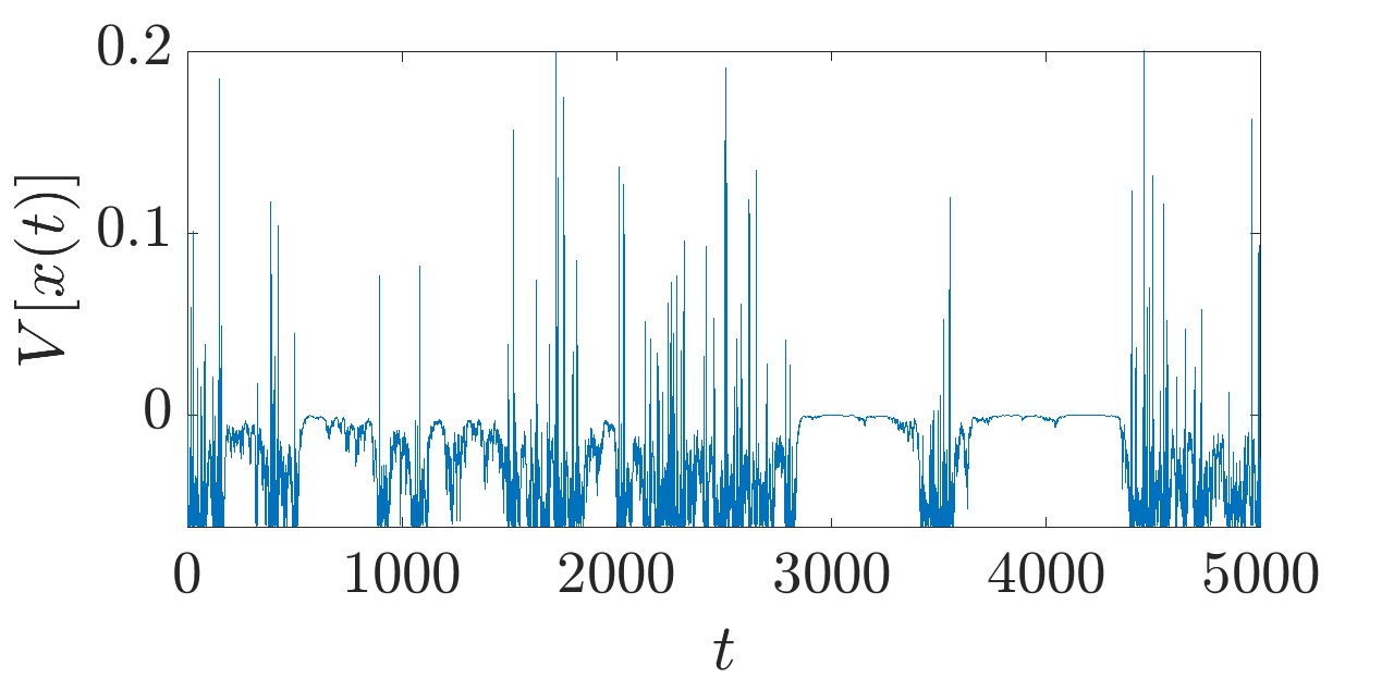
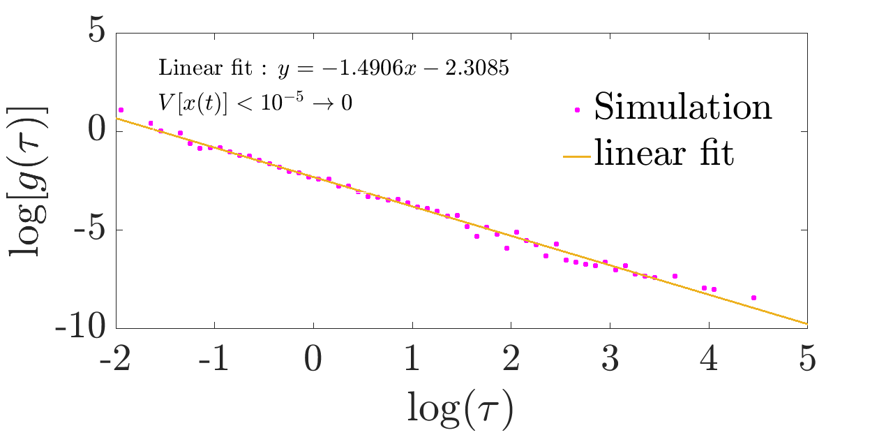
Figure 10: Upper panel: Simulated time series of the potential energy of a particle in the Lennard-Jones potential Eq. (11). It exhibits long periods during which ${|V[x(t)]|<\epsilon}$, where ${\epsilon>0}$ can be as small as we wish, and short periods where the absolute value of the energy is high. Small absolute values of the potential energy corresponds to events where the particle strays far away from the potential minimum (the particle being in the range ${x\gg 1}$). Lower panel: The probability distribution ${g(\tau)}$ of the durations (${\tau}$s) of the time periods where the absolute value of the energy is lower than ${\epsilon=10^{-5}}$ (here, the total measurement time was ${t=2\times 10^{6}}$). ${\log[g(\tau)]}$ versus ${\log(\tau)}$, obtained from the simulation (magenta circles), is matched with a linear fit (orange line) with a slope of ${\approx-3/2}$, which implies that ${g(\tau)}$ has a power-law shape similar to free Brownian motion.

The time-average $\overline{{\cal}O[x(t)]}$ in the time-independent canonical setting is equal to the ensemble-average, in the long-time limit (ergodicity). In our case, the time-averages fluctuate between different trajectories, which is a common theme in single-molecule experiments, and here we explore the fluctuations. To start, we again consider the indicator function, ${\cal O}[x(t)]=I(x_{1}<x(t)<x_{2})$, defined in Eq. (51). However, our results are far more general than that. As we will show, the fluctuations of time-averages of observables integrable with respect to the non-normalized Boltzmann density follow a universal law, in the spirit of the Aaronson-Darling-Kac theorem Aaronson [1997].

For simplicity, let us consider $x_{1}=0$. The process $I(x_{1}<x(t)<x_{2})$, starting inside the region $(0,x_{2})$, is switching randomly between two states, with sojourn times in the interval close to the surface denoted $\tau^{{\rm in}}$, when $I(x_{1}<x(t)<x_{2})=1$, and $\tau^{{\rm out}}$, when $I(x_{1}<x(t)<x_{2})=0$. The first time interval in the domain $(0,x_{2})$ is denoted $\tau_{1}^{{\rm in}}$, and the rest follow, so the sojourn times in the two states are given by the sequence

$$\left\{\tau^{{\rm in}}_{1},\tau^{{\rm out}}_{1},\tau^{{\rm in}}_{2},\tau^{{\rm out}}_{2},\cdots\right\}.$$ (64)

These times can be treated as mutually independent, identically distributed random variables, since temporal correlations in the Langevin Eq. (1) decrease exponentially fast in time. We denote the probability density functions of out and in sojourn times with $\psi_{{\rm out/in}}(\tau)$, respectively. Importantly, in the long-time limit; $\psi_{{\rm out}}(\tau)\propto\tau^{-3/2}$. This well-known result is related of course to the flatness of the potential field at large ${x}$. In this regime, the process $x(t)$ is controlled by diffusion and while it is recurrent, so the density $\psi_{{\rm out}}(\tau)$ is normalized, the average sojourn time in the out state diverges. This absence of a typical timescale, together with the diverging partition function, are precisely the reasons for the failure of the standard (Birkhoff) ergodic theory, and the emergence of Boltzmann-like infinite ergodic theory. The sojourn times in the in state are thinly distributed and, importantly, the moments of $\tau^{\textrm{in}}$ are finite, which is clearly the case since the interval $(0,x_{2})$ is of finite length.

Let $n$ be the number of switching events from the in to the out states. For a fixed measurement time $t$, this number is random. We claim that the distribution of $n$ is determined by the statistics of the ${out}$ times, when $t$ is large. Roughly speaking, the ${in}$ sojourn times are very short when compared to the ${out}$ times, since those have an infinite mean. This means that in the time interval $(0,t)$, we will typically observe an ${out}$ sojourn time of the order of magnitude of the measurement time $t$, and the size of this largest interval controls the number of ${out}$-to-${in}$ transitions (if the largest out time is very long, then $n$ is small, compared with a realization with a shorter maximal out time).

Note that the time-average of $I(x_{1}<x(t)<x_{2})$ is equal to the sum of the in times, divided by the measurement time; $\overline{I}=\sum_{i=1}^{n}\tau_{i}^{{\rm in}}/t$, where we assume, without any loss of generality, that at time $t$ the process is in state out. The mean $\langle\overline{I}\rangle$ was already obtained rigorously from the non-normalized density in Eq. (57), but with the notations of renewal theory we have $\langle\overline{I}\rangle\simeq\langle\tau^{{\rm in}}\rangle\langle n\rangle/t$ and since $\langle n\rangle\sim t^{1/2}$ we have $\langle\overline{I}\rangle\propto t^{-1/2}$, as we found earlier. The behavior $\langle n\rangle\propto t^{1/2}$ is well known in renewal theory, and with a hand-waving argument we note that the effective average sojourn time is $\langle\tau_{{\rm eff}}\rangle=\int_{0}^{t}\tau\psi_{{\rm out}}(\tau){\rm d}\tau\propto t^{1/2}$, and hence $\langle n\rangle\sim t/\langle\tau_{{\rm eff}}\rangle\propto t^{1/2}$.

Let us now consider the second moment of the time-average. Since, for any ${i\neq j}$, ${\langle(\tau^{\rm in}_{i})^{2}\rangle=\langle(\tau^{\rm in}_{j})^{2}\rangle}$ and ${\langle\tau^{\rm in}_{i}\tau^{\rm in}_{j}\rangle=\langle\tau^{\rm in}_{i}\rangle^{2}}$, we argue that

$$\langle\overline{I}^{2}\rangle ={\langle\left(\sum_{i=1}^{n}\tau_{i}^{{\rm in}}\right)^{2}\rangle\over t^{2}}$$

$$={\langle n\rangle\langle(\tau^{{\rm in}})^{2}\rangle+\langle n(n-1)\rangle\langle\tau^{{\rm in}}\rangle^{2}\over t^{2}}.$$ (65)

Now we are ready to get to the main point of this section. Considering the variance of the time-average

$$\langle(\overline{I})^{2}\rangle-\langle\overline{I}\rangle^{2}={\langle(t_{r})^{2}\rangle-\langle t_{r}\rangle^{2}\over t^{2}}=$$

$${\langle n^{2}\rangle-\langle n\rangle^{2}\over t^{2}}\langle\tau^{{\rm in}}\rangle^{2}+{\langle n\rangle\over t^{2}}\underbrace{\left[\langle(\tau^{{\rm in}})^{2}\rangle-\langle\tau^{{\rm in}}\rangle^{2}\right]}_{\textrm{Var}(\tau^{\rm in})},$$ (66)

we see that the second term is negligible, compared with the first, since from renewal theory we know that $n\sim t^{1/2}$. This means that the fluctuations of $\tau_{{\rm in}}$ are irrelevant, and there is a single important timescale describing the process, which is the average sojourn time $\langle\tau^{{\rm in}}\rangle$. We now normalize the variance using $\langle\overline{I}\rangle\sim\langle n\rangle\langle\tau^{{\rm in}}\rangle/t$ and find

$${\langle\overline{I}^{2}\rangle-\langle\overline{I}\rangle^{2}\over\langle\overline{I}\rangle^{2}}\rightarrow{\langle n^{2}\rangle-\langle n\rangle^{2}\over\langle n\rangle^{2}}.$$ (67)

This analysis can be continued to higher order moments and it yields

$${\overline{I}\over\langle\overline{I}\rangle}\rightarrow{n\over\langle n\rangle}\equiv\eta.$$ (68)

This means that the residence time in $(x_{1},x_{2})$, divided by the mean residence time, is equal in a statistical sense to number of the in-to-out transitions over their mean.

The probability density function of $0<\eta$ is known from renewal theory Godreche and Luck [2001], and since $\psi_{{\rm out}}(\tau)\propto\tau^{-3/2}$ we find

$$\mbox{PDF}(\eta)={2\over\pi}e^{-\eta^{2}/\pi}.$$ (69)

This has, by definition, unit mean. Naively, the reader might be tempted to believe that this result is related to the Gaussian central limit theorem. However, this is not the case, since for sojourn-time distributions with other fat tails we will get a form very different from Gaussian He et al. [2008]; Akimoto, Shinkai, and Aizawa [2015]; Aghion, Kessler, and Barkai [2019]. In-fact, ${\mbox{PDF}(\eta)}$ is a special case of a more general density function known as the Mittag-Leffler distribution, which in turn is related to Lévy statistics. Note, that the Aaronson-Darlin-Kac theorem Aaronson [1997] predicts that the distribution of the time average of a process with an infinite measure, will be given by the Mittag-Leffler distribution in the form of $\mathscr{M}_{\alpha}(\eta)=\frac{\Gamma^{1/\alpha}(1+\alpha)}{\alpha\eta^{1+1/\alpha}}l_{\alpha,0}\left[\frac{\Gamma^{1/\alpha}(1+\alpha)}{\eta^{1/\alpha}}\right]$, with ${l_{\alpha,0}(\#)}$ being the one-sided Lévy density (defined as the inverse-Laplace transform of ${\exp(-u^{\alpha})}$, from ${u\rightarrow\#}$), see e.g., Korabel and Barkai [2009]; Akimoto and Barkai [2013]; Radice et al. [2020]. The exponent ${\alpha}$, we argue, is determined by the first return probability ${\psi_{{\rm out}}(\tau)\propto\tau^{-1-\alpha}}$, and in our case, ${\alpha=1/2}$ means that ${\mathscr{M}_{1/2}(\eta)}$ is equal to Eq. (69). Other values of ${\alpha}$ are found in the case of diffusion in logarithmic potentials, as explained in Ref. Aghion, Kessler, and Barkai [2019] (see also Dechant et al. [2011]), which are out of the scope of this manuscript, but in that case a derivation of the Mittag-Leffler distribution can also be made following the same lines as presented below.

A hand-waving argument for Eq. (69), works as follows: Consider $n$ independent, identically distributed random variables ${\tau^{\textrm{out}}_{1},...\tau^{\textrm{out}}_{n}}$, which correspond in our physical model to the times in the state ${out}$. According to the Lévy central limit theorem Metzler and Klafter [2000], the probability density function (PDF) of these times is the one-sided Lévy density with index $1/2$

$$l_{1/2,0}(\tau)={1\over 2\sqrt{\pi}}\tau^{-3/2}\exp\left(-{1\over 4\tau}\right).$$ (70)

Here, like $\psi_{{\rm out}}(\tau)$, $l_{1/2,0}(\tau)\propto\tau^{-3/2}$ and this fat-tailed behavior allows us to consider a specific choice of the ${out}$ times distribution, in the sense that asymptotically the results are not sensitive to the short $\tau$ behavior of $\psi_{\textrm{out}}(\tau)$. We use dimensionless units, and since eventually we consider the dimensionless variable $\eta$, this is not a problem. The Laplace transform ${LT[f(\tau)]=\int_{0}^{\infty}f(\tau)\exp(-\tau u)\textrm{d}\tau}$ of Eq. (70) is $\exp(-u^{1/2})$. Now, consider the random variable $y=\sum_{i=1}^{n}\tau_{i}/n^{2}$. The PDF of $y$ is also the one-sided stable law Eq. (70), since it is easy to check that $\langle\exp(-uy)\rangle=\exp(-u^{1/2})$. We are interested in the probability distribution of $n$, and we fix the measurement time $t$ to be the sum of the sojourn times $t=\sum_{i=1}^{n}\tau_{i}$. Hence $y=t/n^{2}$, and

$$\mbox{PDF}(n)=\mbox{PDF}(y)|{{\rm d}y\over{\rm d}n}|=$$

$$l_{1/2,0}\left({t\over n^{2}}\right)|{2t\over n^{3}}|={1\over\sqrt{\pi t}}\exp\left(-{n^{2}\over 4t}\right).$$ (71)

Thus the density of $n$ is half a Gaussian. From here, we find $\langle n\rangle=2\sqrt{t/\pi}$, and switching to the random variable $\eta=n/\langle n\rangle$ we get Eq. (69). Throughout this derivation, we treat $n$ as a continuous variable, which makes sense in the long-time limit, and can be justified using well-known rigorous results.

We note that, mathematically, the number of switching events $n$ is formally infinite. This is related to the fact that the Langevin trajectories are continuous, hence once we have one transition, we experience many of them. This is not a major problem since we actually considered the scaled random variable $\eta=n/\langle n\rangle$ which has a unit mean. To put it differently, since $\langle n\rangle\sim t^{1/2}$ in the long-time limit, we consider a scaled variable which is perfectly well behaved. From the measurement point of view, we sample the trajectory with a finite rate, so $n$ is always finite, and this is also true in simulations, where we use discrete steps in space and time (in the limit of large ${n}$, the results will not be sensitive to the sampling rate and the discretization).

Inspired by infinite ergodic theory, we claim that the Mittag-Leffler distribution of time-averages is a far more general result. For example, consider the time-average of the potential energy $\overline{V}$. Also here the observable $V[x(t)]$ is switching between long periods where it is nearly zero (when the particle is far in the bulk), to relatively short bursts when this observable is nonzero, when the particle is close to the surface. Again the statistics of the number of times that the particle visits the domain where $V(x)$ is non-negligible, is similar to that of $n$, and its statistics is controlled by the first-passage probability density function from the bulk to the vicinity of the wall. Again, the latter is the fat-tailed density with the familiar $\tau^{-3/2}$ law that we have just mentioned above. So we have

$${\overline{{\cal O}[x(t)]}\over\langle\overline{{\cal O}[x(t)]}\rangle}\rightarrow\eta,$$ (72)

and Eq. (69) still holds. Note that this yields a complete description of the problem in the sense that $\langle\overline{{\cal O}}\rangle$ is calculated in principle with the non-normalized Boltzmann density, and we assume that the observable is integrable with respect to this state.

In the upper panel of Fig. 10, we see a simulated sample of the time series of the potential energy, of a particle in a Lennard-Jones potential (the details of the simulation are similar to Fig. 4). The time series exhibits long periods where ${|V(x)|<\epsilon}$, and ${\epsilon}$ is some lower cutoff that can be as small as we wish, and short periods of high energy (in absolute value). In the lower panel of Fig. 10, we see that the probability distribution ${g(\tau)}$ of the durations (${\tau}$s) of the events where the energy is low, which correspond to events where the particle has strayed far away from the potential minimum, has a power-law shape ${g(\tau)\propto\tau^{-3/2}}$, at large ${\tau}$ (as seen from the fitting function, in an orange line), like in free Brownian motion, as expected. Hence the process is recurrent, but the mean-return time is infinite. In this example, we used ${\epsilon=10^{-5}}$. We verified the Mittag-Leffler distribution of several observables, including the potential energy, using various numerical simulations, whose results are presented in our previous paper, Ref. Aghion, Kessler, and Barkai [2019].

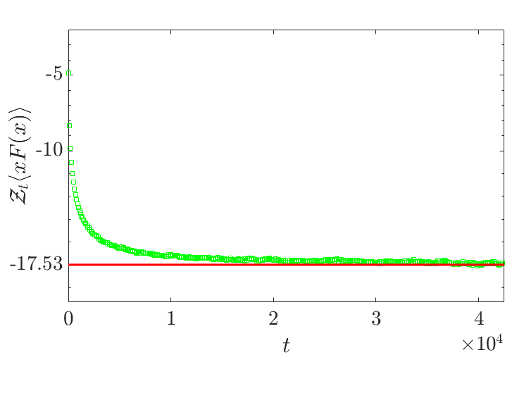
Figure 11: The value of ${\mathcal{Z}_{t}\langle xF(x)\rangle}$, obtained from simulation results based on numerical integration over the Langevin Eq. (1), where ${F(x)=-V^{\prime}(x)}$, and ${V(x)=(-25x^{2}+x^{4}/2)\exp(-x^{2}/20)/125}$ (green circles), approaches at increasing times to the theoretical value given by Eq. (74). Here ${\mathcal{Z}_{t}=2\sqrt{\pi Dt}}$, since the potential is symmetric. ${\gamma=1}$, and ${D=k_{B}T=0.5}$.

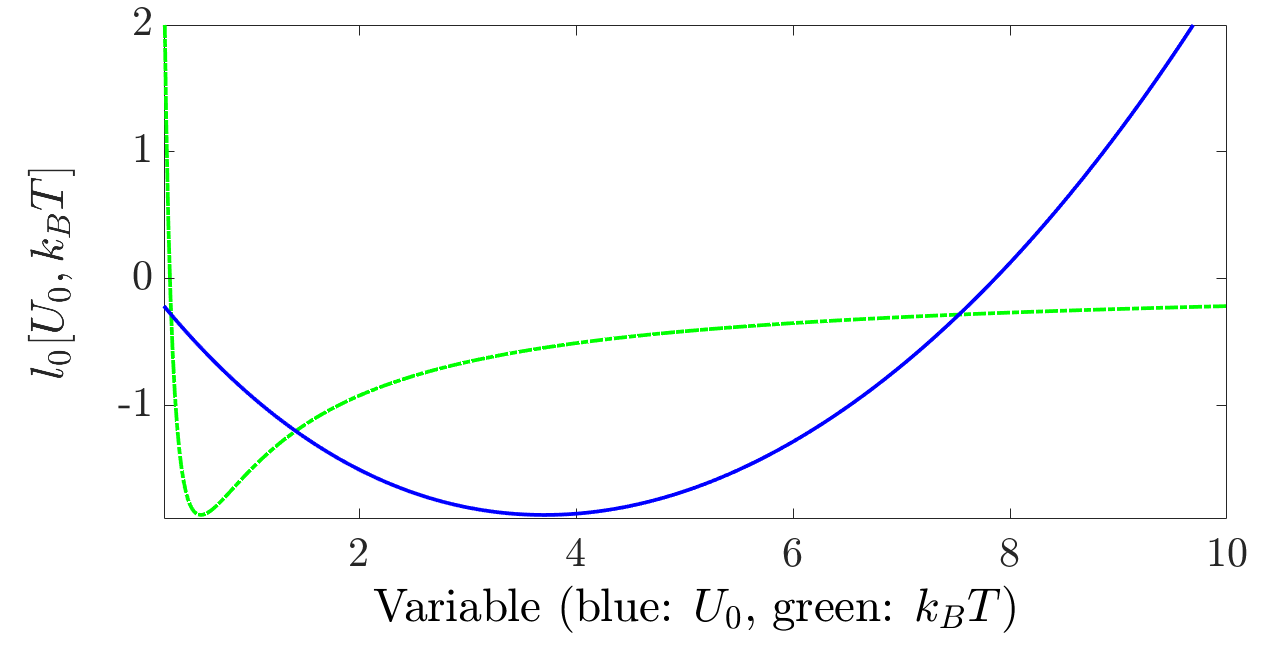
Figure 12: (Color online). Various values of ${l_{0}}$, obtained for the potential ${U(x,U_{0})=U_{0}\left[(-x/5)^{4}-(x/5)^{2}\right]\exp\left[(-x/5)^{2}\right]}$, which change sign for various values of the amplitude ${U_{0}}$ (blue line), at fixed temperature: ${k_{B}T=1}$, as well as for a fixed ${U_{0}=2}$, and varying ${T}$ (green line).

VIII Virial Theorem

The virial theorem addresses the mean of the observable $xF(x)$, where $F(x)=-V^{\prime}(x)$. binding potentials, treated with standard thermodynamics, yield $\langle{xF(x)}\rangle=-k_{B}T$. In our case Aghion, Kessler, and Barkai [2019], using the non-normalized Boltzmann state we find, by integration by parts

$$\langle xF(x)\rangle ={k_{B}T\over\mathcal{Z}_{t}}\int_{0}^{\infty}x{\partial\over\partial x}\left(e^{-V(x)/k_{B}T}-1\right){\rm d}x=$$

$$-{k_{B}T\over\mathcal{Z}_{t}}\int_{0}^{\infty}\left(e^{-V(x)/k_{B}T}-1\right){\rm d}x,$$ (73)

where we used our convention $\exp[-V(\infty)/k_{B}T]=1$. Now, using ${\ell_{0}=\int_{0}^{\infty}[\exp(-V(x)/k_{B}T)-1]\textrm{d}x}$ (introduced in Sec. V), we get

$$\lim_{t\rightarrow\infty}\mathcal{Z}_{t}\langle xF(x)\rangle\rightarrow-k_{B}T{\ell_{0}}.$$ (74)

The ratio $\ell_{0}/\mathcal{Z}_{t}$ distinguishes Eq. (74) from the standard thermal virial theorem, where the ratio ${-\langle xF(x)\rangle/k_{B}T}$ at equilibrium is unity. Note that

$${\ell_{0}=-2{B}_{2},}$$ (75)

where ${{B}_{2}}$ is called the second virial coefficient Chandler [1987]. For two-sided, symmetric potentials ${\langle xF(x)\rangle=-2k_{B}T\ell_{0}/\mathcal{Z}_{t}}$ (but as mentioned, also ${\mathcal{Z}_{t}\rightarrow 2\mathcal{Z}_{t}}$). The constant ${l_{0}}$ points to a surprising link between the virial theorem and the corrections to the uniform approximation, studied in Sec. V (particularly, Eq. (49) for large ${x}$), which means that by measuring the shape of the tails of the diffusing particle packet, one can, at least in principle, obtain knowledge about the force in the system, even though in the large ${x}$ region it is effectively zero. Interestingly, notice that ${\ell_{0}}$ can change sign, for various potentials, which is also very different from standard thermodynamics. Fig. 11 shows the approach of the simulated value of ${\mathcal{Z}_{t}\langle xF(x)\rangle}$ where ${F(x)=-V^{\prime}(x)}$, and ${V(x)=(-25x^{2}+x^{4}/2)\exp(-x^{2}/20)/125}$ at increasing times (green circles), to the theoretical limit, Eq. (74) (red line) with ${k_{B}T=\gamma=0.5}$, where the value is negative. This result was obtained from the overdamped Langevin Eq. (1). In Fig. 12, we show the various values of ${l_{0}}$, obtained for the potential ${U(x,U_{0})=U_{0}\left[(x/5)^{4}-(x/5)^{2}\right]\exp\left[(-x/5)^{2}\right]}$, for various values of the amplitude ${U_{0}}$ (blue line), at fixed temperature: ${k_{B}T=1}$, as well as for a fixed ${U_{0}=2}$, and varying ${T}$ (green line). In both those cases we used ${\gamma=1}$.

VIII.1 A Correction term for the mean-squared displacement, and the underdamped Langevin process

The result of the previous subsection provides us with a nice example that demonstrates that the next-to-leading order correction term, derived for the uniform approximation of ${P_{t}(x)}$ in Sec. V, has also some relevance to thermodynamics. This link is made by looking at the correction term to the linear behavior, in time, of the mean-squared displacement ${\langle x^{2}\rangle}$ of the system, which we now derive using an elementary calculation, and then explain it in terms of the virial theorem.

Using Eq. (49), we get

$$\langle x^{2}\rangle\approx\int_{0}^{\infty}\frac{x^{2}}{\sqrt{\pi Dt}}e^{-x^{2}/(4Dt)}\textrm{d}x$$

$$\qquad\qquad-\int_{0}^{\infty}\frac{x^{2}e^{-x^{2}/(4Dt)}}{\sqrt{\pi Dt}}\left[\frac{\ell_{0}x}{2Dt}\right]\textrm{d}x$$

$$=2Dt-4{\ell_{0}}\sqrt{Dt/\pi},$$ (76)

where we used the fact that at large ${x}$, ${V(x)\approx 0}$. In the above derivation, we considered the integration limits to be zero and infinity, although Eq. (49) is exact only in the large ${x}$ limit, since the contribution to the mean-squared displacement from the small ${x}$ regime is negligibly small at the long-time limit. Fig. 13 shows numerical results corresponding to overdamped Langevin dynamics with the same potential used for all the figures in Sec. V, with ${k_{B}T=\gamma=1}$, which confirm the validity of the correction term to the leading-order, linear, behavior of the second moment in time. The figure also shows an additional constant coming from higher-order correction terms, which was obtained numerically. Note that in the case of a two-sided system, there might be additional correction terms to the mean-squared displacement, of order ${\sqrt{t}}$, if the initial position of the particle is not located at the origin. The reason is that, here, the correction terms to ${P_{t}(x)}$ might differ from Sec. V.

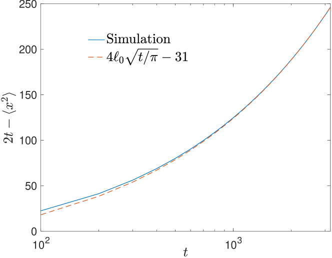
Figure 13: (Color online) Numerical results (blue line), corresponding to overdamped Langevin dynamics with the same potential used for all the figures in Sec. V, with ${k_{B}T=\gamma=1}$), which confirm the validity of the correction term to the leading-order, linear, behavior of the second moment in time. The fitting curve is shown in orange-dashed line, and it corresponds to the ${\sqrt{t}}$ term in Eq. (76), plus an additional constant coming from higher-order correction terms, which was obtained numerically.

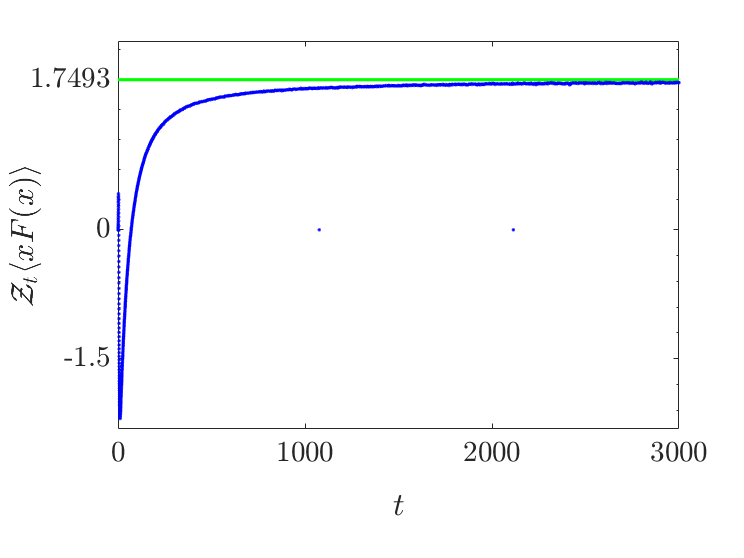
Figure 14: (Color online) The approach of  ${\mathcal{Z}_{t}\langle xF(x)\rangle}$ obtained from simulation results corresponding to the underdamped Langevin process with the two-sided potential Eq. (12), with ${k_{B}T=0.8}$ and ${\gamma=0.5}$, at increasing times (blue circles) to the asymptotic theoretical value Eq. (74) (green line).

To understand the connection between Eq. (76) and the virial theorem, we need to extend our analysis to the phase space and consider both the particle’s position ${x}$, and it’s velocity ${v}$. Namely, in what follows, instead of Eq. (1) we now use the underdamped Langevin equation, with zero-mean, white Gaussian noise; $m\partial_{t}v=F(x)-\gamma v+\eta(t)$. In this process, which also obeys the fluctuation-dissipation relation, ${\gamma>0}$, and we include the acceleration term according to Newton’s second law, where $m$ is the particle’s mass. The analysis below will yield the same results regardless if ${V(x)}$ is a one-sided or two-sided potential, given that the process starts at ${x(t=0)=0}$. Consider the identity

$$m\partial_{t}\langle xv\rangle=m\langle v^{2}\rangle+m\langle x\partial_{t}v\rangle.$$ (77)

Since the velocity is thermalised $m\langle v^{2}\rangle=k_{B}T$, and since $\langle x\eta(t)\rangle=0$ we get

$$m\partial_{t}\langle xv\rangle=k_{B}T+\langle xF(x)\rangle-\gamma\langle xv\rangle,$$ (78)

where clearly

$$\langle xv\rangle={\partial_{t}\langle x^{2}\rangle\over 2}.$$ (79)

Furthermore, we assume that in the long-time limit

$$\langle x^{2}\rangle\sim 2Dt+D_{\beta}t^{\beta}+...,$$ (80)

where the second term is small compared with the first. It is then clear that $|m\partial_{t}\langle xv\rangle|\ll|\gamma\langle xv\rangle|$ and hence

$$\gamma\langle xv\rangle=k_{B}T+\langle xF(x)\rangle.$$ (81)

For equilibrium situations, i.e. for binding potentials like the Harmonic oscillator, $\langle xv\rangle=0$ since the marginal position density is described by the Boltzmann distribution, and Maxwell-distribution for the velocities. This means that in thermal equilibrium, the velocities are not correlated with the spatial position of the particle, since in the single particle Hamiltonian the kinetic energy is separated from the potential energy. For the case under study here, the correlation $\langle xv\rangle$ is not strictly zero.

Coming back to Eq. (81), we see that the term $\langle xF(x)\rangle$ decays like $t^{-1/2}$, since $\mathcal{Z}_{t}\propto t^{1/2}$. Using the leading order term $\langle xv\rangle=\partial_{t}\langle x^{2}\rangle/2\sim D$, from Eq. (81) we get in the very long-time limit $k_{B}T-\gamma D=0$, recovering the Einstein relation. Hence we need to consider the sub-leading terms. It is easy to see that since $\langle xF(x)\rangle\propto t^{-1/2}$ we must have $\beta=1/2$. Using Eqs. (79,80,81) we find

$$\langle xF(x)\rangle={D_{1/2}\gamma\over 4t^{1/2}},$$ (82)

and from Eq. (74)

$$D_{1/2}=-{4\sqrt{D}\ell_{0}\over\sqrt{\pi}}.$$ (83)

It follows that $D_{1/2}$ is determined by the potential energy via the length-scale $\ell_{0}$, and for a given $D$ it is independent of the mass of the particle. Using Eq. (83) in Eq. (80), we therefore recover the first and second leading order terms in ${\langle x^{2}\rangle}$, obtained in Eq. (76). Fig. 14 shows the approach of the mean ${\langle xF(x)\rangle}$ obtained from simulation results, using the underdamped Langevin equation with the potential Eq. (12), to the asymptotic value Eq. (74).

We remark that the observable $xv$ is non-integrable with respect to the non-normalized Boltzmann-Gibbs state. In phase space, we speculate that the non-normalized state is $\exp[-H/k_{B}T]/\mathcal{Z}_{t}$ where the Hamiltonian $H=p^{2}/2m+V(x)$ and $p=mv$ as usual. The only change here is that $\mathcal{Z}_{t}$ is now $\sqrt{\pi Dt}\sqrt{2\pi mk_{B}T}$, where the factor $\sqrt{2\pi mk_{B}T}$ stems from the Maxwell distribution. This expression describes the bulk fluctuations of the packet of particles in phase space, while in the far tails the correlation between $x$ and $v$ builds up. The full analysis of the phase-space infinite-density remains out of the scope of this manuscript.

IX Non-normalizable Boltzmann-Gibbs states in $d$-dimensions

So far, we have treated only one-dimensional processes. However, as we mentioned in the introduction, the issue of the non-normalizability of the Boltzmann factor raised by Fermi was in the context of three-dimensional motion, under the influence of a Coulomb potential Fermi [1924]. We now show that the non-normalizable Boltzmann-Gibbs state is found also in $d$-dimensions, when the external potential is isotropic, and it decays at least as rapidly as ${1/r}$, at large distances. One should keep in mind here that in $2$-dimensions, in the absence of any potential field, Polya’s theorem states that a Brownian particle still returns to its origin with probability ${1}$ (and the mean first return time is infinite), but in any dimension ${d>2}$, this is no longer the case, if the system size is infinite. This holds also in the presence of Coulomb-like potentials. Still, as we now show, the Boltzmann infinite density is valid.

We begin our analysis in the absence of any force. The radial motion of a Brownian particle in ${d}$-dimensions, in the space defined by the orthogonal directions ${\chi_{1},\chi_{2},...\chi_{d}}$, is described by Bessel process Kubo, Toda, and Hashitsume [2012]

$${\dot{r}=D\frac{d-1}{r}+\sqrt{2D}\Gamma(t),}$$ (84)

where ${r=\sqrt{\chi_{1}^{2}+\chi_{2}^{2}+...\chi_{d}^{2}}.}$ Accordingly, the radial Fokker-Planck equation describing the expansion of the probability density ${W_{t}(r)}$ in ${d}$ dimensions is Kubo, Toda, and Hashitsume [2012] ${{\partial_{t}}W_{t}(r)=D\left[((d-1)/r)\partial_{r}+\partial^{2}_{r}\right]W_{t}(r),}$ where ${\int_{0}^{\infty}W_{t}(r)1r^{d-1}\textrm{d}r=1}$ and ${c(d)}$ is a constant which rises from the integration over all the angular degrees of freedom of the ${d}$-dimensional Laplacian. Here we assumed that the initial distribution of the particles was also isotropic around the origin. Substituting

$${W_{t}(r)=P_{t}(r)r^{1-d}/c(d),}$$ (85)

yields

$${\frac{\partial}{\partial t}P_{t}(r)=D\left[\frac{\partial}{\partial r}\frac{{1-d}}{r}+\frac{\partial^{2}}{\partial r^{2}}\right]P_{t}(r),}$$ (86)

where ${\int_{0}^{\infty}P_{t}(r)\textrm{d}r=1}$. The solution to this equation, for various boundary conditions, is found e.g. in Bray [2000]; Martin, Behn, and Germano [2011]; Medalion et al. [2016]. In two dimensions, for example, starting from a ring-shaped initial distribution $P_{0}(r,\phi)=\delta(r-r_{0})\Theta(0<\phi<2\pi)/(2\pi r_{0}),$ with a reflecting boundary condition at ${r=0}$ (see details in Bray [2000]), at time ${t}$ we find $P_{t}(r)\approx({r}/{2Dt})\exp\left(-({r^{2}+r_{0}^{2}})/{4Dt}\right)I_{0}\left({rr_{0}}/{2Dt}\right),$ where ${I_{\nu}(\cdot)}$ is the Bessel function with index ${\nu}$ (and here ${\nu=0}$). In ${d}$-dimensions, starting from a uniform probability distribution on a ${d}$-dimensional sphere of radius ${r_{0}}$, and a reflecting boundary condition at ${r=0}$ Bray [2000]:

$${P_{t}(r)=\frac{r_{0}}{2Dt}\left(\frac{r}{r_{0}}\right)^{d/2}\exp\left(-\frac{r^{2}+r_{0}^{2}}{4Dt}\right)I_{d/2-1}\left(\frac{rr_{0}}{2Dt}\right).}$$ (87)

Below, we add to the system an asymptotically flat potential field, with a repelling part on the origin. In that case, the right-hand side of Eq. (87) will describe the shape of the density in the large ${r}$ regime, where ${V(r)\sim 0}$. One can easily verify, for example, that when ${d=1}$ and ${r_{0}\ll t^{1/2}}$, but $r\sim\mathcal{O}(t^{1/2})$, ${P_{t}(r)}$ in Eq. (87) is $\sim\frac{1}{\sqrt{\pi Dt}}\exp(-r^{2}/(4Dt))$ (as is well known Bray [2000]).

IX.1 The infinite-invariant density

Consider an isotropic, radially dependent potential ${V(r)}$, such that ${V(0)={\infty}}$ and ${V(\infty)={0}}$, which falls-off at least as rapidly as ${1/r}$ at large distances (in the same spirit as the potentials we investigated in the unidimensional case). Now, the radial dynamics is described by

$${\dot{r}=D\frac{(d-1)}{r}-\frac{V^{\prime}(r)}{\gamma}+\sqrt{2D}\Gamma(t).}$$ (88)

As in the unidimensional Langevin equation, Eq. (1), here ${D=k_{B}T/\gamma}$ and ${k_{T},\gamma>0}$. The corresponding radial Fokker-Planck equation is

$${{\frac{\partial}{\partial t}}W_{t}(r)=D\left[\frac{d-1}{r}\frac{\partial}{\partial r}+r^{1-d}\frac{\partial}{\partial r}r^{d-1}\frac{V^{\prime}(r)}{k_{B}T}+\frac{\partial^{2}}{\partial r^{2}}\right]W_{t}(r).}$$ (89)

Here, and in what follows, we assume that the initial particle distribution is narrow, and isotropic. After repeating the substitution from Eq. (85), this yields

$${\frac{\partial}{\partial t}P_{t}(r)=D\left[\frac{\partial}{\partial r}\frac{{1-d}}{r}+\frac{\partial}{\partial r}\frac{V^{\prime}(r)}{k_{B}T}+\frac{\partial^{2}}{\partial r^{2}}\right]P_{t}(r).}$$ (90)

To solve Eq. (90) to leading order, in the long-time limit, we use the ansatz ${P_{t}(r)\approx\frac{r_{0}}{2Dt}\left(\frac{r}{r_{0}}\right)^{d/2}\exp\left(-\frac{r^{2}+r_{0}^{2}}{4Dt}\right)I_{d/2-1}\left(\frac{rr_{0}}{2Dt}\right)\mathcal{I}(r),}$ where ${\mathcal{I}(r)}$ is some general function of ${r}$. Note that this approach is similar to that employed in the unidimensional case, in Sec. III. Plugging this ansatz in Eq. (90), we obtain the uniform approximation

$${P_{t}(r)\approx\frac{r_{0}}{2Dt}\left(\frac{r}{r_{0}}\right)^{d/2}e^{-\frac{r^{2}+r_{0}^{2}}{4Dt}}I_{d/2-1}\left(\frac{rr_{0}}{2Dt}\right)e^{-\frac{V(r)}{k_{B}T}},}$$ (91)

for long ${t}$. From the uniform approximation, Eq. (91), using the asymptotic shape of the Bessel function in the limit ${t\rightarrow\infty}$, since $I_{d/2-1}\left(\frac{rr_{0}}{2Dt}\right)\approx({rr_{0}})^{d/2-1}/\left((4{Dt})^{d/2-1}\Gamma(d/2)\right)$, and ${\exp[-(r^{2}+r_{0}^{2})/(4Dt)]\rightarrow 1}$, we find

$${\lim_{t\rightarrow\infty}{\mathcal{Z}_{t}}r^{1-d}P_{t}(r)\rightarrow\exp\left(-V(r)/k_{B}T\right),}$$ (92)

where ${{\mathcal{Z}}_{t}=2^{d/2-1}\Gamma(d/2)(2Dt)^{d/2}}$. Importantly, from this relation we again see that, in the long time limit, the non-normalizable solution is independent of ${r_{0}}$. In one dimension, from this result we recover Eq. (18).

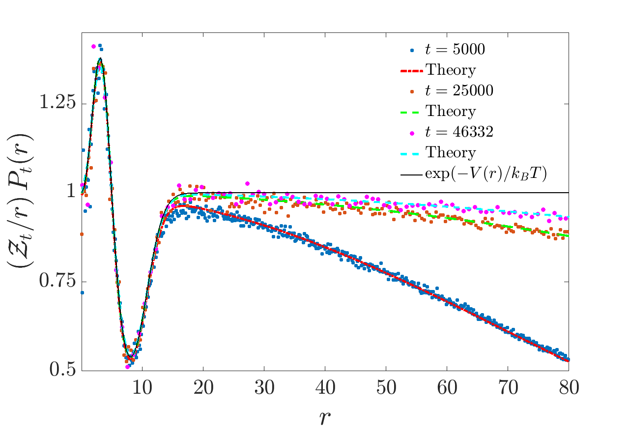
Figure 15: (Color online) Simulation results for a two-dimensional Langevin process, with ${V(r)}$ in Eq. (93) (${\gamma=1}$, and ${k_{B}T=D=0.5}$), compared with theory. Colored symbols: ${(\mathcal{Z}_{t}/r)P_{t}(r)}$, where ${r=\sqrt{x^{2}+y^{2}}}$, ${\mathcal{Z}_{t}=2Dt}$ (see Eq. (92)) and ${P_{t}(r)}$ is the radial distribution, obtained from the simulation at times ${t=5000,25000,46322}$ (blue circles, orange squares and magenta circles, respectively). The corresponding theoretical curves obtained from Eq. (91) with ${d=2}$ (multiplied by ${2Dt/r}$) are the red dash-dot line and a green dashed line and cyan dashed-line. The non-normalizable Boltzmann factor ${\exp(-V(r)/k_{B}T)}$, appears in solid black line. Here, the initial distribution of the ${10^{6}}$ particles was uniform around a ring of radius ${r_{0}=5}$.

Fig. 15 shows excellent agreement between the simulation results of a two-dimensional Langevin process, and the theory corresponding to Eqs. (91,92). The simulation method used an Euler-Mayurama integration scheme over the two Langevin equations $\dot{x}=-V^{\prime}(r)\cos(\theta)+\sqrt{2D}\Gamma_{1}(t)$ and $\dot{y}=-V^{\prime}(r)\sin(\theta)+\sqrt{2D}\Gamma_{2}(t)$, where

$${V(r)=\left[(r/5)^{4}-(r/5)^{2}\right]\exp[-(r/5)^{2}].}$$ (93)

${\Gamma_{1}(t)}$ and ${\Gamma_{2}(t)}$ represent two independent, zero-mean and ${\delta}$-correlated Gaussian white noise terms. At ${t=0}$, the particles were uniformly distributed around a ring of radius ${r_{0}=5}$. Fig. 16 shows simulation results of a three-dimensional Langevin process, with the Coulomb-type potential

$${V(r)=(2/r)^{12}-0.5/r.}$$ (94)

Here ${r}$ is defined in spherical coordinates. The repulsive part of the potentials, which falls-off as rapidly as ${1/r^{12}}$, was added to regularize the interactions near the origin in the simulation (this is technically simpler to realize numerically than putting a hard spherical wall around some ${r\ll 1}$). This model mimics a field created by a finite-sized charge, which repels the observed particle at short distances. The figure shows excellent match between the simulated radial PDF ${P_{t}(r)}$, multiplied by ${\mathcal{Z}_{t}}$ (defined in Eq. (92)) at times ${t=5000,50000,100000}$ (green stars, blue circles and red diamonds, respectively), and the corresponding uniform approximation, Eq. (91) with ${d=3}$ (magenta, purple and brown lines, respectively). At increasing times, the simulation results approach the non-normalizable Boltzmann state ${\exp(-V(r)/k_{B}T)}$ (black line), via Eq. (92), as expected, confirming the existence of the infinite-invariant density also in three dimensions. Here, ${D=k_{B}T=0.05}$. In this system the minimum of the field is on ${r_{\textrm{min}}\approx 2.84}$, hence in Fig. 16 we see a peak at this value. Also notice that the depth of the well is ${V(r_{\textrm{min}})\approx-0.16}$, hence ${V(r_{\textrm{min}})/k_{B}T\approx-3.22}$. Thus we are dealing here with a trap that is not too deep, this allows the escape of the particles on a finite observation time. For a deeper well, we will need to wait for even longer observation time to find the infinite density.

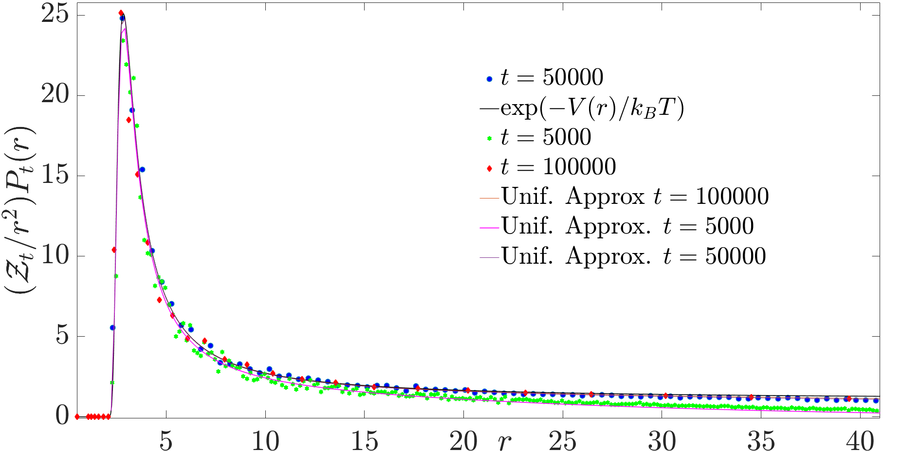
Figure 16: (Color online) Simulation results of a three-dimensional Langevin process, with the Coulomb-type potential Eq. (94). The figure shows excellent match between the simulated radial PDF ${P_{t}(r)}$ (here we used spherical coordinates), multiplied by ${\mathcal{Z}_{t}/r^{2}}$ (and ${{\mathcal{Z}}_{t}}$ is defined below Eq. (92)) at times ${t=5000,50000,100000}$ (green stars, blue circles and red diamonds, respectively), and the corresponding uniform approximation , Eq. (91) with ${d=3}$ (magenta, purple and brown lines, respectively). At increasing times, the simulation results approach to the non-normalizable Boltzmann state ${\exp(-V(r)/k_{B}T)}$ (black line), via Eq. (92), as expected, confirming the existence of the infinite-invariant density also in three dimensions. Here, ${D=k_{B}T=0.05}$, and we used ${10^{7}}$ particles.

IX.2 Ergodicity of time-weighted observables, in $d$-dimensions

As mentioned above, Brownian motion in $d$-dimensions is non-recurrent. In this section, we propose a new approach for evaluating time and ensemble averages of observables integrable with respect to the infinite-density, Eq. (92), and show that this method leads to a Birkhoff-like equality between the two means, which is valid in any dimension ${d\geq 1}$.

Let ${\mathcal{O}(r)}$ be an integrable observable, with respect to ${r^{d-1}\exp\left(-V(r)/k_{B}T\right)}$, in Eq. (92), e.g., ${\mathcal{O}(r)=\Theta(r_{a}<r(t)<r_{b})}$. Here, ${\Theta(r_{a}<r(t)<r_{b})=1}$ while the particle’s trajectory passes inside the $d$-dimensional shell with inner radius ${r_{a}>0}$, and outer radius ${r_{b}<\infty}$, and zero otherwise. We define the ensemble mean of the weighted time-average as

$$\left\langle\overline{\mathcal{Z}_{t}\mathcal{O}[r(t)]}\right\rangle\equiv\left\langle\frac{1}{t}\int_{0}^{t}\mathcal{Z}_{\tilde{t}}\mathcal{O}[r(\tilde{t})]\textrm{d}\tilde{t}\right\rangle$$

$$=\frac{1}{t}\int_{0}^{t}\mathcal{Z}_{\tilde{t}}\left\langle\mathcal{O}(r)\right\rangle_{\tilde{t}}\textrm{d}\tilde{t}=\frac{1}{t}\int_{0}^{t}\textrm{d}\tilde{t}\mathcal{Z}_{\tilde{t}}\int_{0}^{\infty}\mathcal{O}(r)P_{\tilde{t}}(r)\textrm{d}r.$$ (95)

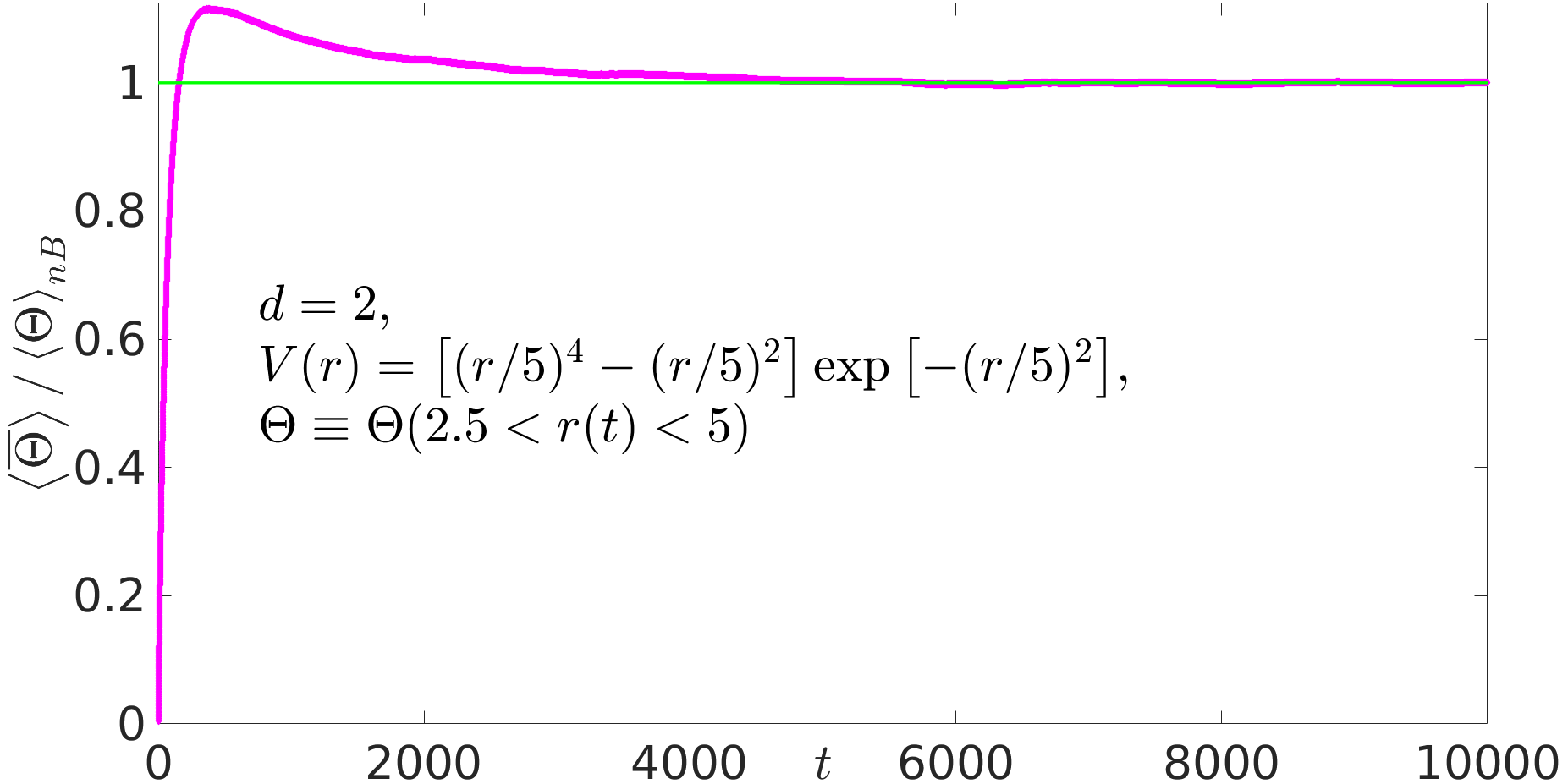
Figure 17: (Color online) The ratio between the weighted time average Eq. (95), measured in a two-dimensional Langevin simulation, and the ensemble average with respect to the non-normalizable Boltzmann state ${\langle\Theta\rangle_{nB}}$ of the indicator function ${\Theta(2.5<r(t)<5)}$, converges to unity at increasing times (simulation results in magenta line, the green line on ${1}$ serves as a guide to the eye). This validates Eq. (98). The details of the simulation are similar to those in Fig. 15 (so ${\langle\Theta\rangle_{nB}\approx 11.7076}$).

Using Eq. (92), in the limit ${t\rightarrow\infty}$, Eq. (95) leads to

$$\left\langle\overline{\mathcal{Z}_{t}\mathcal{O}[r(t)]}\right\rangle \rightarrow\frac{1}{t}\int_{0}^{t}\textrm{d}\tilde{t}\mathcal{Z}_{\tilde{t}}\left[\frac{1}{\mathcal{Z}_{\tilde{t}}}\right]\int_{0}^{\infty}\mathcal{O}(r)r^{d-1}e^{-V(r)/k_{B}T}\textrm{d}r,$$

$$=\int_{0}^{\infty}\mathcal{O}(r)r^{d-1}e^{-V(r)/k_{B}T}\textrm{d}r.$$ (96)

We denote ${\langle\mathcal{O}(r)\rangle_{nB}\equiv\int_{0}^{\infty}\mathcal{O}(r)r^{d-1}e^{-V(r)/k_{B}T}\textrm{d}r,}$ and then Eq. (96) means that when ${t\rightarrow\infty}$, ${\left\langle\overline{\mathcal{Z}_{t}\mathcal{O}[r(t)]}\right\rangle\rightarrow\langle\mathcal{O}(r)\rangle_{nB}}$. We now relate this weighted time average to an ensemble average, performed at time ${t}$. Clearly,

$$\mathcal{Z}_{t}\left\langle{\mathcal{O}(r)}\right\rangle_{t} =\mathcal{Z}_{t}{\int_{0}^{\infty}}\mathcal{O}(r)P_{t}(r)\textrm{d}r$$

$$\rightarrow\langle\mathcal{O}(r)\rangle_{nB}.$$ (97)

Therefore,

$$\lim_{t\rightarrow\infty}\frac{\left\langle\overline{\mathcal{Z}_{t}\mathcal{O}[r(t)]}\right\rangle}{\left\langle{\mathcal{Z}_{t}\mathcal{O}(r)}\right\rangle_{t}}\rightarrow 1.$$ (98)

Eq. (98) is a generalized form of Birkhoff’s theorem. Note that in one dimension, this equation constitutes an alternative to Eq. (62), which was derived for non-weighted time-averages. Here, like in Sec. VI, both the ensemble-average, and the weighted time-average are estimated in the long-time limit from the non-normalizable ($d$-dimensional) Boltzmann-Gibbs state, Eq. (92), hence Eq. (98) constitutes further extension of infinite-ergodic theory (in the sense of the ratio between time and ensemble means). Fig. 17 shows the ratio between the weighted time average Eq. (95), measured in a two-dimensional Langevin simulation, and the ensemble average with respect to the non-normalizable Boltzmann state ${\langle\Theta\rangle_{nB}}$ of the indicator function ${\Theta(2.5<r(t)<5)}$. This ratio converges to unity at increasing times, validating Eq. (98). The details of the simulation are similar to Fig. 15. Fig. 18 shows a similar ratio as in Fig. 17, but this time it is measured in a three-dimensional Langevin simulation, for ${\Theta(2.8<r(t)<3)}$ (blue line). The details of this simulation are similar to Fig. 16, and the ratio again converges to unity at increasing times.

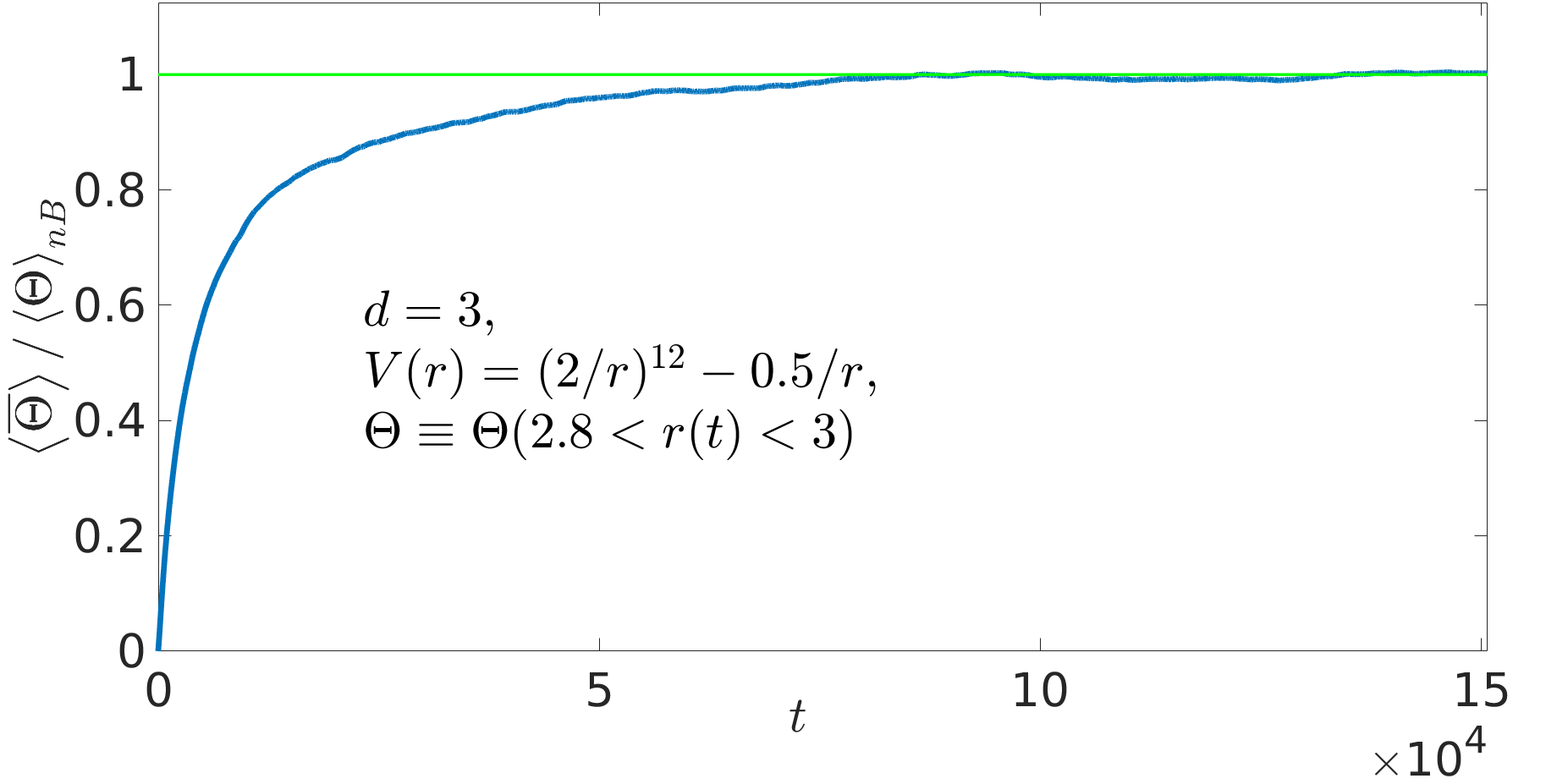
Figure 18: (Color online) The ratio between the weighted time average Eq. (95), measured in a three-dimensional Langevin simulation, and the ensemble average with respect to the non-normalizable Boltzmann state ${\langle\Theta\rangle_{nB}}$ of the indicator function ${\Theta(2.8<r(t)<3)}$, converges to unity at increasing times (simulation results in blue line, the green line on ${1}$ serves as a guide to the eye). This validates Eq. (98). The details of the simulation are similar to Fig. 16 (so ${\langle\Theta\rangle_{nB}\approx 41.7144}$), except that here we used ${10^{5}}$ particles.

X Summary of our main results

In this manuscript, which extends our work in Ref. Aghion, Kessler, and Barkai [2019], we have shown that the spatial shape of a diffusing particle packet, inside an asymptotically flat potential, converges at long times to a non-normalizable Boltzmann state in any dimension, ${d\geq 1}$. This state, which is treated mathematically as an infinite-invariant density Aaronson [1997], takes the place of the standard Boltzmann distribution, which gives the equilibrium state in systems with strong confinement, in the sense that we can use it to obtain time and ensemble averages of integrable observables. We have mainly focused on one-dimensional systems, which obey the Aaronson-Darlin-Kac theorem, and here we also showed that the non-normalizable Boltzmann state gives the entropy-energy relation, and the virial theorem. We studied the emergence of the latter in detail in one dimension, and it would be interesting to study it further also in higher dimensions in a future work.

We have obtained the non-normalizable Boltzmann state in one dimension using three different techniques: via physical scaling assumptions (Sec. III), using the entropy maximization principle (Sec. IV), and via a rigorous eigenfunction expansion method (Sec. V). The last of these also yielded terms which describe the sub-leading order behavior of the probability density function, which decay more rapidly with time. Though the analysis based on an eigenfunction expansion in ${d>1}$ dimension is left for future work, here we showed that by attaching a proper weight function to integrable observables, the ratio between weighted time averages and ensemble averages converges to unity (see Eq. (98)). The distribution of the weighted time average is an open question for future research.

The main results of this manuscript are the uniformly valid approximation for the one-dimensional probability density $P_{t}(x)$ including the first-order correction, Eq. (50); the relationship between the mean-squared position and the virial theorem, expressed in Eq. (76) and Eqs. (80 and 83); the leading order probability density in arbitrary dimensions, Eq. (92); and lastly, the ergodicity of time-weighted observables, expressed in Eq. (98).

XI Discussion

Infinite ergodic theory can be applied to many thermodynamic systems, as the main condition is that the fluctuation-dissipation theorem holds. One must distinguish however between recurrent, and non-recurrent processes, since only in the latter the Aaronson-Darlin-Kac theorem holds. Physically, the key point is that we can identify easily important observables that are integrable with respect to the infinite density, and the fluctuation-dissipation theorem guarantees that this infinite density is the non-normalizable Boltzmann factor. Ryabov, et al. Šiler et al. [2018]; Ryabov, Holubec, and Berestneva [2019] considered a different, though related, setup in one dimension, with an unstable potential that does not allow for the return of the particle to its starting point. Also here the partition function diverges, but again a certain aspect of Boltzmann equilibrium remains. Hence, our work suggests that further aspects of ergodicity should be studied in this setup, perhaps in the spirit of the evaluation of weighted-time-averaged observables, and it also indicates that future studies in that direction could be interesting in other classes of potentials as well. Our work also encourages the investigation of these problems in non-Markovian settings, and in the presence of many-body interactions, and since we have assumed that the fluctuation-dissipation relation holds, it will be interesting to examine if this assumption can be relaxed and infinite-ergodic theory can be studied also e.g. in the framework of active particles, as in Romanczuk et al. [2012]; Hoell, Löwen, and Menzel [2019].

While in this manuscript we considered the fluctuations of time averages, and in particular the fluctuations of energy, the whole framework of stochastic thermodynamics could in principle be investigated. For example, it would be interesting to explore the fluctuations of the rate of entropy production, and the work and heat exchange between the particles and the heat bath. It should be noted however that our theory gives rise to both extensions of stochastic thermodynamics, for systems with a non-normalizable Boltzmann-Gibbs state, but also the connection between fluctuations (diffusivity) and thermodynamics. This is seen in the virial correction to the diffusion law (Sec. VIII). In the current theory, one cannot separate diffusion from non-normalized Boltzmann-Gibbs states, as was demonstrated in the extremum principle studied in Sec. IV.

Acknowledgement: The support of Israel Science Foundation grant $1898/17$ is acknowledged.

References

- Chandler [1987] D. Chandler, Introduction to Modern Statistical Mechanics, by David Chandler, pp. 288. Foreword by David Chandler. Oxford University Press, Sep 1987. ISBN-10: 0195042778. ISBN-13: 9780195042771 , 288 (1987).
- Aghion, Kessler, and Barkai [2019] E. Aghion, D. A. Kessler, and E. Barkai, Physical Review Letters 122, 010601 (2019).
- Darling and Kac [1957] D. Darling and M. Kac, Transactions of the American Mathematical Society 84, 444 (1957).
- Aaronson [1997] J. Aaronson, “An Introduction to Infinite Ergodic Theory” (American Mathematical Soc., 1997).
- Dechant et al. [2011] A. Dechant, E. Lutz, E. Barkai, and D. A. Kessler, Journal of Statistical Physics 145, 1524 (2011).
- Bouin, Dolbeault, and Schmeiser [2020] E. Bouin, J. Dolbeault, and C. Schmeiser, Kinetic & Related Models 13, 345 (2020).
- Wang, Deng, and Chen [2019] X. Wang, W. Deng, and Y. Chen, The Journal of Chemical Physics 150, 164121 (2019).
- Sivan and Farago [2018] M. Sivan and O. Farago, Physical Review E 98, 052117 (2018).
- Šiler et al. [2018] M. Šiler, L. Ornigotti, O. Brzobohatỳ, P. Jákl, A. Ryabov, V. Holubec, P. Zemánek, and R. Filip, Physical review letters 121, 230601 (2018).
- Ryabov, Holubec, and Berestneva [2019] A. Ryabov, V. Holubec, and E. Berestneva, Journal of Statistical Mechanics: Theory and Experiment , 084014 (2019).
- Zweimüller [2009] R. Zweimüller, Lecture notes, Surrey Univ (2009).
- Thaler [2001] M. Thaler, “Infinite ergodic theory. course notes from” the dynamic odyssey”, cirm 2001,” (2001).
- Akimoto and Miyaguchi [2010] T. Akimoto and T. Miyaguchi, Physical Review E 82, 030102 (2010).
- Korabel and Barkai [2012] N. Korabel and E. Barkai, Physical Review Letters 108, 060604 (2012).
- Klages [2013] R. Klages, in From Hamiltonian Chaos to Complex Systems (Springer, 2013) pp. 3–42.
- Akimoto, Shinkai, and Aizawa [2015] T. Akimoto, S. Shinkai, and Y. Aizawa, Journal of Statistical Physics 158, 476 (2015).
- Meyer and Kantz [2017] P. Meyer and H. Kantz, Physical Review E 96, 022217 (2017).
- Leibovich and Barkai [2019] N. Leibovich and E. Barkai, Physical Review E 99, 042138 (2019).
- Akimoto, Barkai, and Radons [2019] T. Akimoto, E. Barkai, and G. Radons, arXiv preprint arXiv:1908.10501 (2019).
- Zhou, Xu, and Deng [2019] T. Zhou, P. Xu, and W. Deng, arXiv preprint arXiv:1909.07213 (2019).
- Sato and Klages [2019] Y. Sato and R. Klages, Physical Review Letters 122, 174101 (2019).
- Radice et al. [2020] M. Radice, M. Onofri, R. Artuso, and G. Pozzoli, Physical Review E 101, 042103 (2020).
- Kessler and Barkai [2010] D. A. Kessler and E. Barkai, Physical Review Letters 105, 120602 (2010).
- Lutz and Renzoni [2013] E. Lutz and F. Renzoni, Nature Physics 9, 615 (2013).
- Rebenshtok et al. [2014a] A. Rebenshtok, S. Denisov, P. Hänggi, and E. Barkai, Physical Review Letters 112, 110601 (2014a).
- Rebenshtok et al. [2014b] A. Rebenshtok, S. Denisov, P. Hänggi, and E. Barkai, Phys. Rev. E 90, 062135 (2014b).
- Holz, Dechant, and Lutz [2015] P. C. Holz, A. Dechant, and E. Lutz, EPL (Europhysics Letters) 109, 23001 (2015).
- Aghion, Kessler, and Barkai [2017] E. Aghion, D. A. Kessler, and E. Barkai, Physical Review Letters 118, 260601 (2017).
- Wang et al. [2019] W. Wang, A. Vezzani, R. Burioni, and E. Barkai, Physical Review Research 1, 033172 (2019).
- Vezzani, Barkai, and Burioni [2019] A. Vezzani, E. Barkai, and R. Burioni, Physical Review E 100, 012108 (2019).
- Pavani et al. [2009] S. R. P. Pavani, M. A. Thompson, J. S. Biteen, S. J. Lord, N. Liu, R. J. Twieg, R. Piestun, and W. Moerner, Proceedings of the National Academy of Sciences 106, 2995 (2009).
- Chechkin et al. [2012] A. V. Chechkin, I. M. Zaid, M. A. Lomholt, I. M. Sokolov, and R. Metzler, Physical Review E 86, 041101 (2012).
- Metzler et al. [2014] R. Metzler, J.-H. Jeon, A. G. Cherstvy, and E. Barkai, Physical Chemistry Chemical Physics 16, 24128 (2014).
- Campagnola et al. [2015] G. Campagnola, K. Nepal, B. W. Schroder, O. B. Peersen, and D. Krapf, Scientific Reports 5, 17721 (2015).
- Krapf et al. [2016] D. Krapf, G. Campagnola, K. Nepal, and O. B. Peersen, Physical Chemistry Chemical Physics 18, 12633 (2016).
- Wang, Wu, and Schwartz [2017] D. Wang, H. Wu, and D. K. Schwartz, Physical Review E 119, 268001 (2017).
- Ashkin et al. [1986] A. Ashkin, J. M. Dziedzic, J. Bjorkholm, and S. Chu, Optics letters 11, 288 (1986).
- Grier and Roichman [2006] D. G. Grier and Y. Roichman, Applied Optics 45, 880 (2006).
- Drobczynski and Ślezak [2015] S. Drobczynski and J. Ślezak, Appl. Opt. 54, 7106 (2015).
- Fermi [1924] E. Fermi, Zeitschrift für Physik 26, 54 (1924).
- Godreche and Luck [2001] C. Godreche and J. Luck, Journal of Statistical Physics 104, 489 (2001).
- He et al. [2008] Y. He, S. Burov, R. Metzler, and E. Barkai, Physical review letters 101, 058101 (2008).
- Korabel and Barkai [2009] N. Korabel and E. Barkai, Physical Review Letters 102, 050601 (2009).
- Akimoto and Barkai [2013] T. Akimoto and E. Barkai, Physical Review E 87, 032915 (2013).
- Metzler and Klafter [2000] R. Metzler and J. Klafter, Physics Reports 339, 1 (2000).
- Kubo, Toda, and Hashitsume [2012] R. Kubo, M. Toda, and N. Hashitsume, “Statistical physics II: nonequilibrium statistical mechanics”, Vol. 31 (Springer Science & Business Media, 2012).
- Bray [2000] A. J. Bray, Physical Review E 62, 103 (2000).
- Martin, Behn, and Germano [2011] E. Martin, U. Behn, and G. Germano, Physical Review E 83, 051115 (2011).
- Medalion et al. [2016] S. Medalion, E. Aghion, H. Meirovitch, E. Barkai, and D. A. Kessler, Scientific Reports 6, 27661 (2016).
- Romanczuk et al. [2012] P. Romanczuk, M. Bär, W. Ebeling, B. Lindner, and L. Schimansky-Geier, The European Physical Journal Special Topics 202, 1 (2012).
- Hoell, Löwen, and Menzel [2019] C. Hoell, H. Löwen, and A. M. Menzel, The Journal of Chemical Physics 151, 064902 (2019).