Experimental investigation of entropic uncertainty relations and coherence uncertainty relations
Abstract
Uncertainty relation usually is one of the most important features in quantum mechanics, and is the backbone of quantum theory, which distinguishes from the rule in classical counterpart. Specifically, entropy-based uncertainty relations are of fundamental importance in the region of quantum information theory, offering one nontrivial bound of key rate towards quantum key distribution. In this work, we experimentally demonstrate the entropic uncertainty relations and coherence-based uncertainty relations in an all-optics platform. By means of preparing two kinds of bipartite initial states with high fidelity, i.e., Bell-like states and Bell-like diagonal states, we carry on local projective measurements over a complete set of mutually unbiased bases on the measured subsystem. In terms of quantum tomography, the density matrices of the initial states and the post-measurement states are reconstructed. It shows that our experimental results coincide with the theoretical predictions very well. Additionally, we also verify that the lower bounds of both the entropy-based and coherence-based uncertainty can be tightened by imposing the Holevo quantity and mutual information, and the entropic uncertainty is inversely correlated with the coherence. Our demonstrations might offer an insight into their uncertainty relations and their connection to quantum coherence in quantum information science, which might be applicable to the security analysis of quantum key distributions.
I INTRODUCTION
Heisenberg’s uncertainty principle Heisenberg172 is deemed as one of the most fundamental features of quantum world, which essentially is different from classical world. The uncertainty principle manifests that it is impossible to accurately predict both the position and the momentum of a microscopic particle. In other words, the more accurate the position measurement is, the more uncertain the momentum measurement will be, and vice versa Coles015002 ; Wang1900124 . Before long, Robertson Robertson163 generalized the uncertainty principle to an arbitrary pair of non-commuting observables. Notably, there is a conceptual shortcoming in Robertson’s inequality, leading to a trivial result when the systemic state is in the state of one of eigenstates of the measured observables. Afterwards, Deutsch had established the celebrated entropic uncertainty relation (EUR) Deutsch631 ; Kraus3070 , in terms of Shannon entropy, which was improved by Maassen and Uffink into the form of Maassen1103
| (1) |
where and are two arbitrary observables, denotes the Shannon entropy, and stands for the maximum overlap between any two eigenvectors ( and ) of and .
Notably, the entropy-based uncertainty relation mentioned previously is suitable for observing the law of incompatible measurements in a single-particle system. As to a composite system with to be probed and as a quantum memory, Berta et al. Berta659 had put forward the quantum-memory-assisted entropic uncertainty relation, which is given by
| (2) |
where represents the conditional von Neumann entropy of and is the reduced state, denotes the conditional von Neumann entropy of the post-measurement state , which can be obtained by performing the local projective measurements on the subsystem . Subsequently, Li et al. Li752 and Prevedel et al. Prevedel757 experimentally demonstrated the quantum-memory-assisted entropic uncertainty relation through two back-to-back all-optical configurations.
Technically, EURs had yielded many potential applications in the domain of quantum information science, e.g., quantum key distribution Berta659 ; Li752 , entanglement witness Berta659 ; Li752 ; Prevedel757 ; Coles022112 , quantum teleportation Hu032338 , quantum steering Schneeloch062103 ; Walborn130402 , and quantum metrology Jarzyna013010 . Accordingly, EURs has received much attention and several tighter lower bounds of the uncertainty were proposed by means of various methods Pati042105 ; Hu014105 ; Coles022112 ; Adabi062123 ; Huang545 . Later on, the entropic uncertainty relations are generalized to multi-observable versions Liu042133 ; Xiao042125 . Soon afterwards, Xing et al. Xing2563 reported an experimental investigation of entropic uncertainty relations with regard to three measurements in a pure diamond system. In addition, there exhibit some promising experiments to verify different types of uncertainty relations Ma160405 ; Xiao17904 ; Wang39 ; Chen062123 .
On the other hand, quantum coherence, the embodiment of the superposition principle of quantum states, is also one of the most fundamental features that marks the violation of quantum mechanics from the classical world Streltsov041003 ; Hu1 ; Vicente045301 ; Marvian052324 . It has been widely concerned and studied since Baumgratz et al. Baumgratz140401 established a rigorous framework for the quantification of coherence. Generally, quantum coherence is related to the characteristics of the whole system. In order to reveal the relationship between quantum coherence and quantum correlations, the unilateral coherence Ma160407 ; Hu052106 is introduced for a bipartite system. Intrinsically, quantum coherence of a quantum state depends on the choice of the reference basis. If two or more incompatible reference bases are selected, coherence-based uncertainty relations (CURs) can be established Singh47 ; Yuan032313 ; Dolatkhah13 ; Fan085203 . Soon after, Lv et al. Lv062337 demonstrated an all-optical experiment of CURs in two different reference bases.
In this paper, we focus on achieving experimental investigations with respect to EURs and CURs in an all-optics framework. By means of preparing two kinds of bipartite initial states, i.e., Bell-like states (pure) and Bell-like diagonal states (mixed), we then perform local projective measurements over a complete set of mutually unbiased bases (MUBs) on one of the subsystem Wootters391 ; Wootters363 . By utilizing quantum tomography James052312 , we obtain the density matrices of the initial states and the post-measurement states, as well as the corresponding measurement probability. It shows our experimental results coincide with the theoretical predictions very well. Moreover, we also demonstrate that the lower bounds of both the entropic and coherence-based uncertainty can be strengthened based on the Holevo quantity and mutual information.
II THEORETICAL FRAMEWORK
Briefly, we herein review the EURs for multiple measurements, and then render a theoretical framework of the CURs. For a quantum state in a -dimensional Hilbert space , once resorting to an arbitrary set of basis , the relative entropy of coherence can be written as Baumgratz140401
| (3) |
where is the von Neumann entropy, and is the diagonal part of in the basis . For a bipartite state in a composite Hilbert space , after performing a local projective measurement on subsystem , the probability of obtaining result is quantified by and the post-measurement state of the bipartite composite system reads as , where is the identity operator in Hilbert space of subsystem . As a result, the post-measurement state of the system is a mixture of , explicitly given by
| (4) |
In general, the unilateral coherence of the bipartite system can be written as Ma160407 ; Hu052106
| (5) |
Furthermore, for a bipartite state and projective measurements performed on subsystem , the entropic uncertainty relations with regard to multiple measurements can be described by Liu042133
| (6) |
here with denoting the largest overlap between any two eigenvectors of the given observables. According to Eqs. (5) and (6), we can obtain the uncertainty relations for unilateral coherence under multiple measurements Dolatkhah13 , viz.
| (7) |
Specifically, for a -dimensional bipartite state , if we select a complete set of MUBs applied on subsystem , the EURs and CURs in MUBs can be derived into
| (8a) | |||
| (8b) | |||
respectively. Note that, the lower bound of the EURs can be strengthened by adding a term relating to the Holevo quantity and mutual information Dolatkhah13 ; Adabi062123
| (9) |
where , is the mutual information of the bipartite system , and is the Holevo quantity Nielsen , which is an upper bound on the accessible information by the local projective measurement on the subsystem . Likewise, this additional term has been verified to be available on improving the lower bound of the CURs Fan085203
| (10) |
III EXPERIMENTAL SCHEME
As an illustration, we herein choose a two-qubit mixed state as the initial state, which is with form of
| (11) |
where and are two Bell-like states with the adjustable parameter , and is an adjustable mixing parameter which is used to change the proportion of the two Bell-like states. Here, is encoded the horizontal polarization state and is encoded the vertical polarization state in a linear optical system KwiatR773 ; Xu7 ; Qi19 ; Wu454 ; Li032107 . For the local projective measurement on the subsystem , we resort to the eigenbasis of three Pauli operators to build a most commonly used complete set of MUBs in a qubit system.
| Operator | Measurement | ||||
|---|---|---|---|---|---|
| HWP | HWP | ||||
| HWP | HWP | ||||
| QWP | QWP | ||||
| QWP | QWP | ||||
| HWP | HWP | ||||
| HWP | HWP |
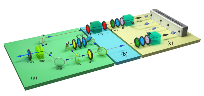
We herein set up an all-optical experiment to realize the scheme, and the schematic diagram of our scheme is provided in Fig. 1. To be explicit, the experimental setup can be divided into three parts: (a) quantum state preparation, (b) local projective measurement, and (c) quantum state tomography. In part (a), we firstly prepare the entangled mixed state shown as Eq. (11). After a continuous linearly polarized pumped beam with the power of 130 mW and the wavelength of 405nm passes through a half-wave plate (HWP), a beam of polarized light with adjustable horizontal and vertical components can be harvested. The parameter can be easily adjusted by changing the angle of the optical axis of the HWP. This pumped beam is focused on two type-I -barium borate (BBO) crystals (mm) with optical axis cut at . After that, a pair of entangled photons with state and the central wavelength of 810nm will be generated by the spontaneous parametric down-conversion (SPDC). In order to prepare the mixed state consisting of two Bell-like state, we add an unbalanced Mach-Zehnder device (UMZ) in the A-path Li752 , which includes two 50/50 beam splitters (BSs), two mirrors (MIRs), two attenuators (ATTs), and two HWPs with optical axes and , respectively. The mixing weight parameter can be regulated by the two ATTs. Part (b) is to realize the local projective measurements of A-path photons. It consists of two wave plates and and a polarizing beam splitter (PBS). By means of different wave plate combinations and setting the corresponding optical axis angles (for ) and (for ), the different projective measurements can be implemented. The detailed setting has been provided in Table I Ding022308 . The role of part (c) is to reconstruct the quantum state by the tomography process, which consists of two quarter-wave plates (QWPs), two HWPs, two 3-nm interference filters (IFs), two PBSs, four single photon detectors (SPDs) and a logic coincidence unit. By setting the optical axis of the QWPs and the HWPs, we can achieve at least 16 groups of measurement bases. Based on the obtained coincidence number, the density matrix of the quantum state can be perfectly reconstructed James052312 .
IV EXPERIMENTAL RESULTS
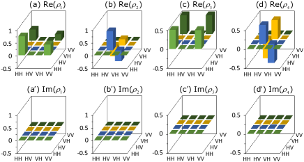
To prepare the initial states given in Eq. (11), we prepare two kinds of states, i.e., Bell-like states (pure) and Bell-like diagonal states (mixed). First, we assure that the parameter is constant, and choose to prepare two groups of Bell-like states: and . In this case, the value of is adopted as , respectively. Second, we fix the parameter and prepare the other two groups of Bell-like diagonal states: and . Here is set as , respectively. We reconstruct the density matrices of all initial states by quantum state tomography process shown in part (c) in Fig. 1. Explicitly, Fig. 2 shows the real and imaginary parts of four typical Bell-like states we prepared: , , , . By precisely adjusting the mixing proportion of these quantum states, we can easily prepare the Bell-like diagonal states as desired by us. In our scheme, the average fidelity of the experimental result is up to , quantified by , where is the corresponding target states, and the error bar is estimated according to the Monte Carlo method Altepeter105 .
With respect to the initial state we prepared, we perform the local complete set of MUB measurements on photon , which are composed of the eigenbases of the three Pauli operators : , and , where is the outcome of 0 or 1. In linear optics, we generally assume that , , , , , and , where , , , and denote the diagonal, antidiagonal, right-circular, and left-circular polarized states Altepeter105 . After the local measurements, the bipartite states will become , and with the corresponding probability , and , respectively. Similarly, we can reconstruct the density matrices of these quantum states according to tomography process, and work out the corresponding probability via coincidence counts Li752 . Thereby, one can attain the post-measurement states of the composite system: , and . To demonstrate the EURs and the CURs we focus, it is indispensable to derive the left-hand sides and the right-hand sides of Eqs. (8a), (8b), (9), and (10), respectively. Explicitly, the left-hand side of Eq. (8a) is defined by , and the left-hand side of Eq. (8b) by . and stand for the right-hand sides of Eqs. (8a) and (8b), and represent the right-hand sides of Eqs. (9) and (10), respectively.
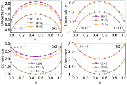
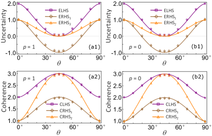
The experimental results and theoretical predictions of the EURs and the CURs in MUBs with the initial Bell-like states and Bell-like diagonal states have been shown in Figs. 3 and 4. The axis in Fig. 3 represents the parameter of the initial states, while the axis in Fig. 4 represents the parameter . In both figures, the axis of subgraphs (a1) and (b1) represents the magnitude of the uncertainty, and the axis of subgraphs (a2) and (b2) represents the values of the coherence. The purple squares in (a1) and (b1) represent the measured values of ELHS and the purple squares in (a2) and (b2) represent CLHS. The brown rhombus and the orange triangles in (a1) and (b1) denote the measured values of and , while these shapes in (a2) and (b2) denote and , respectively. The solid lines with different colors represent the corresponding theoretical predictions of uncertainties and coherences, respectively. Following the figures, it has been directly shown that the experimental results coincide with the theoretical predictions very well, which lies in:
(i) All experimental results are consistent with the theoretical curve within the error range, which not only verifies the theory in an all-optical setup, but also indicates that the prepared quantum states have high fidelity.
(ii) The orange triangles ( or ) are always above the brown rhombus ( or ), which means that the lower bounds of the entropic uncertainty relations and the coherence uncertainty relations can be improved by the Holevo quantity and mutual information. In particular, for Bell diagonal states in Figs. 4 (b1) and (b2), it indicates that the orange rhombus and the purple squares (ELHS or CLHS) almost coincide, meaning that the lower bounds of the EURS and CURs are enhanced.
(iii) With the variation of quantum state parameters, the total entropic uncertainty (ELHS) will increases (decreases), while the total coherence uncertainty (CLHS) decreases (increases). It means that the entropic uncertainty is inversely correlated with the coherence, which is essentially in agreement with the conclusion from Dolatkhah13 . For the Bell-like states and in Figs. 3, the total coherence reaches a maximum of 3 at , while the uncertainty decreases to the minimum value of 0. This phenomenon is also shown in Figs. 4 (b1) and (b2) with Bell diagonal states .
V CONCLUSIONS
To conclude, we experimentally demonstrated the entropic uncertainty relations and the coherence-based uncertainty relations via an all-optical platform. We prepare the initial states in Bell-like states and Bell-like diagonal states with high fidelity . We perform a complete set of MUBs measurements on one of the subsystems, i.e., three general Pauli-operator measurements. By virtue of quantum tomography, we reconstruct the density matrices of the initial states and the post-measurement states, as well as gaining the corresponding measurement probability. Therefore, we can easily attain the magnitude of the uncertainty and the lower bounds in those proposed uncertainty inequalities both experimentally and theoretically. Remarkably, our experimental results coincide with the theoretical predictions very well. Moreover, it also verifies that the lower bounds of these inequalities are effectively improved by means of the Holevo quantity and mutual information. Further, the experimental results also suppose that the entropic uncertainty is inversely correlated with the quantum coherence. With these in mind, we believe that our demonstration could deepen the understanding of entropic uncertainty relations and its connection to quantum coherence, and the results are expected to be applicable to quantum key distributions.
ACKNOWLEDGMENTS
This work was supported by the National Natural Science Foundation of China (Grant Nos. 11575001, 11405171, 61601002 and 11605028), the Natural Science Research Project of Education Department of Anhui Province of China (Grant No. KJ2018A0343), the Key Program of Excellent Youth Talent Project of the Education Department of Anhui Province of China (Grant Nos. gxyqZD2019042, gxyq2018059 and gxyqZD2018065), the Key Program of Excellent Youth Talent Project of Fuyang Normal University (Grant No. rcxm201804), the Open Foundation for CAS Key Laboratory of Quantum Information (Grant Nos. KQI201801 and KQI201701), and the Research Center for Quantum Information Technology of Fuyang Normal University (Grant No. kytd201706).
Zhi-Yong Ding and Huan Yang contributed equally to this work.
References
- [1] W. Heisenberg, Z. Phys. 43, 172 (1927).
- [2] P. J. Coles, M. Berta, M. Tomamichel, and S. Wehner, Rev. Mod. Phys. 89, 015002 (2017).
- [3] D. Wang, F. Ming, M.-L. Hu, and L. Ye, Ann. Phys. (Berlin) 531, 1900124 (2019).
- [4] H. P. Robertson, Phys. Rev. 34, 163 (1929).
- [5] D. Deutsch, Phys. Rev. Lett. 50, 631 (1983).
- [6] K. Kraus, Phys. Rev. D 35, 3070 (1987).
- [7] H. Maassen and J. B. M. Uffink, Phys. Rev. Lett. 60, 1103 (1988).
- [8] M. Berta, M. Christandl, R. Colbeck, J. M. Renes, and R. Renner, Nat. Phys. 6, 659 (2010).
- [9] C.-F. Li, J.-S. Xu, X.-Y. Xu, K. Li, and G.-C. Guo, Nat. Phys. 7, 752 (2011).
- [10] R. Prevedel, D. R. Hamel, R. Colbeck, K. Fisher, and K. J. Resch, Nat. Phys. 7, 757 (2011).
- [11] P. J. Coles and M. Piani, Phys. Rev. A 89, 022112 (2014).
- [12] M.-L. Hu and H. Fan, Phys. Rev. A 86, 032338 (2012).
- [13] J. Schneeloch, C. J. Broadbent, S. P. Walborn, E. G. Cavalcanti, J. C. Howell, Phys. Rev. A 87, 062103 (2013).
- [14] S. P. Walborn, A. Salles, R. M. Gomes, F. Toscano, P. H. Souto Ribeiro, Phys. Rev. Lett. 106, 130402 (2011).
- [15] M. Jarzyna, R. Demkowicz-Dobrzański, New J. Phys. 17, 013010 (2015).
- [16] A. K. Pati, M. M. Wilde, A. R. Usha Devi, A. K. Rajagopal, and Sudha, Phys. Rev. A 86, 042105 (2012).
- [17] M.-L. Hu and H. Fan, Phys. Rev. A 88, 014105 (2013).
- [18] F. Adabi, S. Salimi, and S. Haseli, Phys. Rev. A 93, 062123 (2016).
- [19] J.-L. Huang, W.-C. Gan, Y. Xiao, F.-W. Shu, and M.-H. Yung, Eur. Phys. J. C 78, 545 (2018).
- [20] S. Liu, L.-Z. Mu, and H. Fan, Phys. Rev. A 91, 042133 (2015).
- [21] Y. Xiao, N. Jing, S.-M. Fei, T. Li, X. Li-Jost, T. Ma, and Z.-X. Wang, Phys. Rev. A 93, 042125 (2016).
- [22] J. Xing, Y.-R. Zhang, S. Liu, Y.-C. Chang, J.-D. Yue, H. Fan, and X.-Y. Pan, Sci. Rep. 7, 2563 (2017).
- [23] W. Ma, Z. Ma, H. Wang, Z. Chen, Y. Liu, F. Kong, Z. Li, X. Peng, M. Shi, F. Shi, S.-M. Fei, and J. Du, Phys. Rev. Lett. 116, 160405 (2016).
- [24] L. Xiao, K. Wang, X. Zhan, Z. Bian, J. Li, Y. Zhang, P. Xue, and A. K. Pati, Opt. Exp. 25, 17904 (2017).
- [25] H. Wang, Z. Ma, S. Wu, W. Zheng, Z. Cao, Z. Chen, Z. Li, S.-M. Fei, X. Peng, V. Vedral, and J. Du, npj Quantum Inf. 5, 39 (2019).
- [26] Z.-X. Chen, J.-L. Li, Q.-C. Song, H. Wang, S. M. Zangi, and C.-F. Qiao, Phys. Rev. A 96, 062123 (2017).
- [27] A. Streltsov, G. Adesso, and M. B. Plenio, Rev. Mod. Phys. 89, 041003 (2017).
- [28] M.-L. Hu, X. Hu, J. Wang, Y. Peng, Y.-R. Zhang, and H. Fan, Phys. Rep. 762-764, 1 (2018).
- [29] J. I de Vicente and A. Streltsov, J. Phys. A: Math. Theor. 50, 045301 (2017).
- [30] I. Marvian and R. W. Spekkens, Phys. Rev. A 94, 052324 (2016).
- [31] T. Baumgratz, M. Cramer, and M. B. Plenio, Phys. Rev. Lett. 113, 140401 (2014).
- [32] J. Ma, B. Yadin, D. Girolami, V. Vedral, and M. Gu, Phys. Rev. Lett. 116, 160407 (2016).
- [33] M.-L. Hu and H. Fan, Phys. Rev. A 95, 052106 (2017).
- [34] U. Singh, A. K. Pati, and M. N. Bera, Mathematics 4, 47 (2016).
- [35] X. Yuan, G. Bai, T. Peng, and X. Ma, Phys. Rev. A 96, 032313 (2017).
- [36] H. Dolatkhah, S. Haseli, S. Salimi1, and A. S. Khorashad, Quantum Inf. Process. 18, 13 (2019).
- [37] X.-G. Fan, Z.-Y. Ding, H. Yang, J. He, and L. Ye, Laser Phys. Lett. 16, 085203 (2019).
- [38] W.-M. Lv, C. Zhang, X.-M. Hu, H. Cao, J. Wang, Y.-F. Huang, B.-H. Liu, C.-F. Li, and G.-C. Guo, Phys. Rev. A 98, 062337 (2018).
- [39] W. K. Wootters, Found. Phys. 16, 391 (1986).
- [40] W. K. Wootters, B. D. Fields, Ann. Phys. 191, 363 (1989).
- [41] D. F. V. James, P. G. Kwiat, W. J. Munro, and A. G. White, Phys. Rev. A 64, 052312 (2001).
- [42] M. A. Nielsen and I. L. Chuang, Quantum Computation and Quantum Information (Cambridge University Press, Cambridge, 2000).
- [43] P. G. Kwiat, E. Waks, A. G. White, I. Appelbaum, and P. H. Eberhard, Phys. Rev. A 60, R773 (1999).
- [44] J.-S. Xu, X.-Y. Xu, C.-F. Li, C.-J. Zhang, X.-B. Zou, and G.-C. Guo, Nat. Commun. 1, 7 (2010).
- [45] B. Qi, Z. Hou, Y. Wang, D. Dong, H.-S. Zhong, L. Li, G.-Y. Xiang, H. M. Wiseman, C.-F. Li, and G.-C. Guo, npj Quantum Inf. 3, 19 (2017).
- [46] K.-D. Wu, Z. Hou, H.-S. Zhong, Y. Yuan, G.-Y. Xiang, C.-F. Li, and G.-C. Guo, Optica 4, 454 (2017).
- [47] J. Li, C.-Y. Wang, T.-J. Liu, and Q. Wang, Phys. Rev. A 97, 032107 (2018).
- [48] Z.-Y. Ding, H. Yang, H. Yuan, D. Wang, Jie Yang, and L. Ye, Phys. Rev. A 100, 022308 (2019).
- [49] J. B. Altepeter, E. R. Jeffrey, and P. G. Kwiat, Adv. At. Mol. Opt. Phys. 52, 105 (2005).