Bridging Inertial and Dissipation Range Statistics in Rotating Turbulence

Abstract

We investigate the connection between the inertial range and the dissipation range statistics of rotating turbulence through detailed simulations of a helical shell model and a multifractal analysis. In particular, by using the latter, we find an explicit relation between the (anomalous) scaling exponents of equal-time structure functions in the inertial range in terms of the generalised dimensions associated with the energy dissipation rate. This theoretical prediction is validated by detailed simulations of a helical shell model for various strengths of rotation from where the statistics of dissipation rate, and thus the generalised dimensions, as well as the inertial range, in particular the anomalous scaling exponents, are extracted. Our work also underlines a surprisingly good agreement—such as in the spatial structure of the energy dissipation rates and the decrease in inertial range intermittency with increasing strengths of rotation—between solutions of the Navier–Stokes equation in a rotating frame with those obtained from low-dimensional, dynamical systems such as the shell model which are not explicitly anisotropic. Finally, we perform direct numerical simulations of the Navier–Stokes equation, with the Coriolis force incorporated, to confirm the robustness of the conclusions drawn from our multifractal and shell model studies.

I Introduction

Turbulent flows are amongst the more well-known problems where the use of standard tools of statistical physics and analysis has met with limited success. One of the factors contributing to this is the intermittent nature of the flow Frisch (1995); Lohse and Grossmann (1993) which, in turn, leads to non-Gaussian distributions of observables such as velocity gradients as well as the multiscaling of (suitably-defined) $q$-th order moments of the spatial increments of the velocity field: Higher-order moments (and their exponents $\zeta_{q}$) are not trivially (linearly) related to lower-order moments Kolmogorov (1941a, b, 1962). We recall that these moments, referred to as equal-time structure functions, and the associated exponents, for a velocity field ${\bf v}({\bf x})$ are defined as $S_{q}(r)\equiv\langle\delta v\,^{q}\rangle\sim r^{\zeta_{q}}$, where $\delta v\equiv[{\bf v}({\bf x}+{\bf r})-{\bf v}({\bf x})]\cdot{\bf\hat{r}}$. The angular brackets denote an average over the spatial points ${\bf x}$; the separation ${\bf r}$ over which this velocity difference is taken (and then projected along that vector ${\bf\hat{r}}$ to obtain the longitudinal component) is assumed to be within the inertial range of scales of turbulence. In other words $L\gg r\gg\eta$, where $L$ is the largest scales where energy is injected and $\eta$ is the smallest (Kolmogorov) length scales where energy is dissipated. Several experiments and direct numerical simulations (DNSs) of the three-dimensional, incompressible Navier-Stokes equation for fully-developed, statistically homogeneous and isotropic turbulence have now established beyond doubt that not only are distributions of velocity-gradients and fluid acceleration characterised by non-Gaussianity and fat tails Kailasnath, Sreenivasan, and Stolovitzky (1992); La Porta et al. (2001) but the scaling exponents $\zeta_{q}$ are non-linear, concave, monotonically increasing functions of $q$.

While the inertial range exponents display multiscaling, there is also overwhelming experimental and numerical evidence Batchelor and Townsend (1949) that the energy dissipation rates show strong temporal and spatial fluctuations Siggia (1981) characterized by periods of intense bursts and calmness. An important question is to find rigorous estimates for the statistics of the energy dissipation rate $\epsilon$ which is, within the Kolmogorov picture, on average equal to the constant energy flux across the inertial range of scales. A popular candidate to model the statistics of $\epsilon$ is to use a log-normal form to fit the probability distribution function of the energy dissipation rate Kolmogorov (1962). Subsequently, this issue of the statistics of the dissipation rate has been revisited and the problems associated with the log-normal assumption Mandelbrot (1972); Kraichnan (1974) eventually gave way to fractal models Mandelbrot (1974); Frisch, Sulem, and Nelkin (1978) culminating in the Frisch–Parisi multifractal formalism Frisch and Parisi (1985). One of the great successes of the latter was the rationalization of the observed multiscaling of velocity structure functions Frisch (1995); Pandit, Perlekar, and Ray (2009).

This connection between the statistics of the dissipation and inertial ranges has been studied extensively for turbulence which is homogeneous and isotropic. However, a similar analysis and its consequences when isotropy is explicitly broken is far from obvious. In this work, we explore this question in some detail by studying turbulent flows in a setting where isotropy is explicitly broken. A natural choice for this is the problem of rotating turbulence Greenspan (1968); Moffatt (1983); Davidson (2013) whose ubiquity ensures that our study is not merely an academic exercise but an important addition in areas of fluid dynamics, geophysics, and astrophysics Barnes (2001); Cho et al. (2008); Le Reun et al. (2017); Aurnou et al. (2015). Indeed there are several examples of turbulent flows which are inevitably associated with the Coriolis force that, while doing no work or additional energy injection, reorganizes the structure of the flow, introduces anisotropy and hence leads to physics quite distinct (often mediated by large-scale columnar vortices) from non-rotating turbulent flows Smith and Waleffe (1999); Müller and Thiele (2007); Mininni, Alexakis, and Pouquet (2009); Bartello (1995); Métais et al. (1996); Yarom, Vardi, and Sharon (2013). Thus, unsurprisingly, the last few decades have seen major theoretical and experimental studies on the different Lagrangian and Eulerian aspects of rotating turbulence Bartello, Métais, and Lesieur (1994); Bartello (1995); Métais et al. (1996); Godeferd and Lollini (1999); Zeman (1994); Hattori, Rubinstein, and Ishizawa (2004); Müller and Thiele (2007); Mininni, Alexakis, and Pouquet (2009); Sreenivasan and Davidson (2008); Pouquet and Mininni (2010); Castello and Clercx (2011); Biferale et al. (2016); Maity, Govindarajan, and Ray (2019); Ibbetson and Tritton (1975); Hopfinger, Browand, and Gagne (1982); Bewley et al. (2007); Morize, Moisy, and Rabaud (2005); Moisy et al. (2011); Yarom, Vardi, and Sharon (2013); Yarom, Salhov, and Sharon (2017); Sharma et al. (2018); Sharma, Verma, and Chakraborty (2018, 2019). Surprisingly, though, the issue of the statistics of the Eulerian dissipation field (beyond a recent work on Lagrangian irreversibility) and its connections with the observed modifications of the statistics of the inertial range, quantified via the scaling exponents of the equal-time structure functions, has not been studied in-depth for such flows Seiwert, Morize, and Moisy (2008); Thiele and Müller (2009); Mininni and Pouquet (2010a); Imazio and Mininni (2017).

In this paper, we tackle this question. In particular, we (a) show how with increasing rotation rates not only does the energy dissipation field appear less intermittent with associated changes in its multifractal spectrum, and (b) establish a relation between the anomalous exponents of equal-time velocity structure functions, measured in the inertial range to the Rényi scaling exponent obtained from partition functions of the dissipation field $\varepsilon(x)$.

Experiments and DNSs are of course primary sources on which theoretical and phenomenological ideas are built. Nevertheless, synthetic models still serve as useful tools to develop insights on the origins of intermittency and the curious nature of energy dissipation Kraichnan (1958, 1959); Orszag (1970); Lesieur (2008); Frisch and Bec (2001); Saha, Chakraborty, and Bhattacharjee (2008); Chakraborty, Saha, and Bhattacharjee (2009); Ray (2015, 2018). A particularly useful example of this is the class of cascade models known as shell models. Remarkably such models which have very little in common (beyond the formal structure) to the Navier–Stokes equations, are shown, for homogeneous and isotropic turbulence, to mimic the multiscaling of two-point correlation functions with remarkable accuracy and hence have, over the years, proved a remarkable testing ground for theories of various correlation functions which were inaccessible to full-scale simulations or experiments.

Rotating turbulent flows are however inherently anisotropic. Therefore, for such systems, understandably, the use of shell models have been sparse. Therefore, in this work, beyond our theoretical (multifractal) analysis, we resort to extensive simulations of a shell model which incorporates the effect of the Coriolis force without explicitly resolving the anisotropy which manifests itself through structural differences in the flow in planes parallel and perpendicular to the axis of rotation. Nevertheless, as we find, such a shell model is still robust enough to (a) pick out the relevant Zeman scales and hence the two power-law regimes in the energy spectrum, (b) predict the scaling exponents of the equal-time structure functions (without, of course, distinguishing the planes parallel and perpendicular to the axis of rotation) in the inertial range with significant accuracy, and (c) allow an extraction of the spatial profile of the energy dissipation rate, through a method due to Lepreti, Carbone, and Veltri Lepreti, Carbone, and Veltri (2006). The last of these allows us to extract the generalised dimension $D_{q}$ for the dissipation rate statistics which, coupled with measurements of $\zeta_{q}$, serves to independently verify the validity of our theoretical prediction bridging the statistics of the inertial and the dissipation ranges. In the end, we finally resort to full-scale direct numerical simulations of the Navier–Stokes equation, with rotation, as well as results from DNSs reported by others in the past, to validate of the central results of our shell model study. This agreement between the two approaches not only underlines one of the objectives of this work, viz., the extent and usefulness of modeling rotating turbulence as a low-dimensional dynamical systems model, but it also serves as an additional confirmation of the theoretical predictions borne out of the multifractal approach.

II A Helical Shell Model for Rotating Turbulence

We begin with the incompressible ($\mathbf{\nabla}\cdot\mathbf{u}=0$) Navier–Stokes equation for the velocity field $\mathbf{u}$ of a three-dimensional flow, with density $\rho$ and a kinematic viscosity $\nu$ small enough to generate turbulence, under a solid body rotation $\mathbf{\Omega}$:

$$\frac{\partial\mathbf{u}}{\partial t}+(\mathbf{u}.\mathbf{\nabla})\mathbf{u}=-\frac{1}{\rho}\mathbf{\nabla}p+\nu\nabla^{2}\mathbf{u}-2\mathbf{\Omega}\times\mathbf{u}+\mathbf{f}.$$ (1)

The pressure $p$ includes the effect of the centrifugal force and the Coriolis force $-2\mathbf{\Omega}\times\mathbf{u}$ results from the solid body rotation. Furthermore, an external, large-scale, force $\mathbf{f}$ ensures that the (turbulent) flow remains in a statistically stationary state through the injection of an energy $\epsilon=\langle\mathbf{u}\cdot\mathbf{f}\rangle$. Unlike non-rotating three-dimensional turbulent flows, helicity plays an important role in rotating turbulence; a natural source of helicity is the Coriolis force which results in a helicty injection $\langle 2\mathbf{u}\cdot\nabla(\mathbf{\Omega}\cdot\mathbf{u})\rangle$; similarly the external drive can also inject helicity at large-scales via helicity $\langle\omega\cdot\mathbf{f}+\mathbf{u}\cdot(\nabla\times\mathbf{f})\rangle$. (The angular brackets in these definitions imply suitable averaging in space or in time for non-equilibrium stationary states.)

The solution of Eq. (1) is characterized not only by its Reynolds number $Re$ (as would be the case for non-rotating flows) but by a second non-dimensional number, the Rossby number $Ro=\mathbf{u}_{\rm rms}/(2L\mathbf{\Omega})$, which is a measure of the relative importance of the Coriolis and inertial terms in flow; $L$ is the characteristic length of the domain (typically, 2$\pi$ in numerical simulations) and $\mathbf{u}_{\rm rms}$ is the root-mean-square velocity.

Rotating turbulent flows in nature or in laboratories have often a non-zero helicity. This non-zero helicity, in turn, affects the statistical properties of the flow principally through a modification of the fluxes. Given that in this paper we bridge inertial to dissipative range statistics, it is useful to avoid possible (non-essential) contributions coming in via a mean helicity. Thus, we are careful in ensuring a zero mean-helicity injection in the model we simulate (see below); we have nevertheless checked that small to moderate mean helicities do not change the central results of this paper.

Shell models are essentially low-dimensional dynamical systems which mimic the spectral Navier–Stokes equation without being actually derived from it Frisch (1995); Bohr et al. (1998); Biferale (2003); Pandit, Perlekar, and Ray (2009). The dynamical system is constructed by replacing the three-dimensional Fourier space with a one-dimensional logarithmically-spaced shell-space. We associate with each shell $n$ in this lattice, corresponding to a wavenumber $k_{n}=k_{0}\lambda^{n}$, a dynamical, complex variable $u_{n}$ which mimics the velocity increments over a scale $r\sim 1/k_{n}$ in the Navier–Stokes equation. The actual structure of this shell-space is determined by the constant $k_{0}$ and $\lambda$. It is this logarithmic construction on a one-dimensional lattice and restricting the non-linear interactions to just the nearest and next-nearest neighbours which allows shell models to achieve extremely high Reynolds numbers—and hence inertial ranges—well beyond those possible through DNSs. Curiously, shell models seem to give very reliable measurements of the anomalous, due to intermittency, scaling exponents of structure functions and the energy spectrum; however not much is known about the dissipation statistics of such models. Thus such models have been used extensively in the past for problems which ranged from studies of static and dynamic multiscaling in fluid, passive-scalar, binary fluids and magnetohydrodynamic turbulence Biskamp (1994); Wirth and Biferale (1996); Basu et al. (1998); Frick and Sokoloff (1998); Mitra and Pandit (2004, 2005); Ray, Mitra, and Pandit (2008); Ray and Basu (2011); Banerjee et al. (2013), turbulent flows with polymer-additives and elastic turbulence Benzi et al. (2003); Kalelkar, Govindarajan, and Pandit (2005); Ray and Vincenzi (2016) as well the equilibrium solutions of such dynamical systems Ditlevsen and Mogensen (1996); Gilbert et al. (2002); Tom and Ray (2017). However, the application of such low-dimensional models for rotating turbulence is both sparse and fairly recent Chakraborty, Jensen, and Sarkar (2010); Hattori, Rubinstein, and Ishizawa (2004).

To this end, we simulate a helical shell model (to ensure a zero mean helicity for the reasons mentioned before), for rotating turbulence, constructed by decomposing the velocity field in the basis corresponding to the eigenvectors of the curl operator Benzi et al. (1996); Waleffe (1992):

$$\mathbf{u}(\mathbf{x}) = \sum_{\mathbf{k}}\mathbf{u}(\mathbf{k})\exp(i\mathbf{k}\cdot\mathbf{x})$$ (2)

$$= \sum_{\mathbf{k}}[u^{+}(\mathbf{k})\mathbf{h}_{+}+u^{-}(\mathbf{k})\mathbf{h}_{-}]\exp(i\mathbf{k}\cdot\mathbf{x}).$$

Here $\mathbf{u}^{\pm}$ are the velocity components along the unit eigenvectors $\mathbf{h}_{\pm}$ of the curl operator $i\mathbf{k}\times\mathbf{h}_{\pm}=\pm k\mathbf{h}_{\pm}$. Such a decomposition is adapted to a shell model framework to yield the following set of ordinary differential equations

$$\frac{d}{dt}u_{n}^{\pm}=\mathcal{N}^{\pm}-\nu k_{n}^{2}u_{n}^{\pm}+\mathcal{F}_{m}^{\pm}-i\Omega u_{n}^{\pm}.$$ (3)

The non-linear terms $\mathcal{N}^{\pm}$ are defined as

$$\mathcal{N}^{\pm} = i\left[ak_{n+1}u_{n+2}^{\mp}u_{n+1}^{\pm}+bk_{n}u_{n+1}^{\mp}u_{n-1}^{\pm}\right.$$ (4)

$$\left.+ck_{n-1}u_{n-1}^{\mp}u_{n-2}^{\mp}\right]^{*}$$

with real coefficients $a,b$ and $c$, the superscript * denoting a complex conjugate, and the effective velocity associated with each shell $u_{n}=\sqrt{|u_{n}^{+}|^{2}+|u_{n}^{-}|^{2}}$. We set the coefficient $a$ to unity and the coefficients $b=-\frac{\lambda^{-1}+\lambda}{\lambda+1}$ and $c=\frac{\lambda^{-1}+1}{\lambda+1}$ to ensure the conservation ($\nu=0$) of energy ($a+b+c=0$) and helicity ($a+b\lambda-c\lambda^{2}=0$). The structure of the shell model allows an easy identification of the viscous dissipative term and a forcing term on the $m^{th}$ shell with $\mathcal{F}_{m}^{\pm}=\epsilon^{\pm}(1+i)/(u^{\pm}_{m})^{*}$; $\epsilon^{\pm}$ is the energy input rate to the mode $u_{m}^{\pm}$ and we choose $m=3$. The helicity injection rate is given by $k_{m}(\epsilon^{+}-\epsilon^{-})$; by choosing $\epsilon^{+}=\epsilon^{-}$ we ensure that there is no injection of kinetic helicity in the system. Finally, the last term— where $\Omega$ is the rotation rate—mimics the Coriolis force and is made explicitly imaginary to ensure that it does not explicitly inject energy into the system.

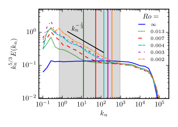
Figure 1: Loglog plots of the compensated energy spectrum $k_{n}^{5/3}E(k_{n})$ versus the wavenumber $k_{n}$ for different Rossby numbers (see legend) from our simulations of the helical shell model. For $Ro=\infty$, the plateau (over several decades and shown by the shaded region) confirms the Kolmogorov scaling $E(k_{n})\sim k_{n}^{-5/3}$ for non-rotating, homogeneous and isotropic turbulence. As the Rossby number decreases, corresponding to an increased level of rotation, the compensated spectrum to the left of the Zeman scale (shown by vertical lines with colors corresponding to the respective $Ro$ numbers) departs from the plateau with an additional scaling factor which asymptotes to $k_{n}^{-1/3}$, and hence $E(k_{n})\sim k_{n}^{-2}$, as $Ro\ll 1$ and for wavenumbers lower than the Zeman wavenumber.

In our simulations, we use a total of $N=32$ shells (with $k_{0}=1/16$ and $\lambda=1.62$), $\nu=10^{-7}$ ($Re\sim 10^{7}$), and for time-marching an exponential fourth-order Runge-Kutta scheme, with a time-step $\delta t=10^{-4}$, to factor in the stiffness of these coupled ordinary differential equations. We initialise our velocity field ($u_{n}^{\pm}=\sqrt{k_{n}}\exp(i\theta)$, for $n\leq 4$ and $u_{n}^{\pm}=\sqrt{k_{n}}\exp(-k_{n}^{2})\exp(i\theta)$ for $n\geq 5$, where $\theta\in[0,2\pi]$ is a random phase) and force the system to a statistically steady state before turning on the Coriolis term.

Analogous to the case of turbulence generated in a rotating fluid governed by the Navier–Stokes equation, the Rossby number is defined as $Ro:=U_{\rm rms}/\Omega L_{0}$, where $U_{\rm rms}=(\sum_{n}\mid u_{n}\mid^{2})^{1/2}$ is the root-mean-square velocity and $L_{0}=1/k_{0}$ is the integral length scale Biferale (2003). We perform simulations with several different values of $Ro$; in this paper, for clarity, we present results mostly for the cases $Ro=\infty$ (no rotation), $0.004,0.003$, and $0.002$ (corresponding to $\Omega=0,10,15$, and $20$, respectively).

III Structure functions in rotating turbulence

The Coriolis force plays a significant effect on the statistics of turbulence. Dimensionally, rotation sets an (inverse) time-scale in the problem resulting in a characteristic (Zeman) scale $l_{\Omega}\sim\sqrt{{\epsilon}/{{\Omega}^{3}}}$ (or wavenumber $k_{\Omega}\sim\sqrt{{{\Omega}^{3}}/{\epsilon}}$) where the rotational and fluid (eddy) turnover time-scales match Zeman (1994). For finitely small values of the Zeman scale (corresponding to $Ro\ll 1$), the two-point statistics, most usefully characterized by the (Fourier space) kinetic energy spectrum $E(k)=|u(k)|^{2}$, shows a dual-cascade Zeman (1994); Zhou (1995); Yeung and Zhou (1998); Baroud et al. (2002, 2003); Hattori, Rubinstein, and Ishizawa (2004); Biferale et al. (2016): For wavenumbers $k<k_{\Omega}$, $E(k)\sim k^{-2}$ and for $k>k_{\Omega}$, the usual Kolmogorov spectrum $E(k)\sim k^{-5/3}$. The dual cascade energy spectrum phenomenology is central to theories of rotating turbulence. It is tempting to now ask if low-dimensional dynamical systems, which mimic the formal structure of the Navier–Stokes equation but are neither rigorously derived from them nor sensitive to the geometrical reorganisation of flows under rotation, show any evidence of this new rotation-induced scaling regime. Remarkably, simulations of the shell model—which is devoid of geometry but only respects the formal structure of the Navier–Stokes equation—shows the exact same scaling behaviour. (For the shell model, the energy spectrum is defined as $E(k_{n})=|u(k_{n})|^{2}/k_{n}$ with an associated Zeman scale defined as above.)

A convenient way to see the point and extent of departure from the Kolmogorov $k^{-5/3}$ scaling is to look at plots of the compensated spectrum $k_{n}^{5/3}E(k_{n})$ versus $k_{n}$, for different strengths of the Coriolis force. In Fig. 1, we present representative plots of this compensated spectra for different values of the Rossby number. For clarity, we show by vertical lines, the Zeman wavenumber corresponding to different values of $Ro$ and shade the inertial range which would have been present in the absence of rotation; for easy comparison we also show results from simulations of non-rotating, homogeneous, isotropic turbulence corresponding to $Ro=\infty$. We immediately note the flatness of the compensated spectrum—before falling-off in the deep dissipation range—for all values of $Ro$ as long as $k_{n}>k_{\Omega}$. This is in sharp contrast to the steeper slopes of the spectrum, as evidenced by the departure from the plateau, for finite rotation ($Ro\neq\infty$) at scales $k_{n}<k_{\Omega}$. In the limit of strong rotation $Ro\ll 1$, the compensated spectrum reaches a slope $E(k_{n})\sim k_{n}^{-1/3}$ (indicated by the black-solid line), for $k_{n}<k_{\Omega}$, corresponding to prediction of the secondary scaling regime $E(k)\sim k^{-2}$ for wavenumbers smaller than the Zeman wavenumber. The dual-scaling behaviour observed in our spectrum is consistent with those observed earlier in fully resolved direct numerical simulations for the so-called isotropic energy spectrum Biferale et al. (2016); Mininni and Pouquet (2010b); Yeung and Zhou (1998), which is obtained by ignoring the rotation-induced anisotropy and averaging over spherical Fourier shells; interestingly, earlier results also suggest that the scaling of this isotropic spectrum is identical to the one obtained from just considering the wavevectors perpendicular to the axis of rotation Thiele and Müller (2009); Mininni and Pouquet (2010b).

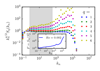
Figure 2: Compensated plots of the equal-time structure functions (compensated by the dimensional prediction $q/2$ for $Ro\to 0$) of various orders for $Ro=0.002$. The shaded region marks the range of inertial scales (lower than the Zeman wavenumber) where rotation modifies the scaling behaviour. The departure from a plateau, especially for higher orders, shows the existence of intermittency corrections to the dimensional prediction. (Inset) A plot of the flatness versus the wave-number as a measure scale-by-scale intermittency for the same value of the Rossby number.

The nature of the energy spectrum from our shell model is consistent with the phenomenology and dimensional predictions which ignore any corrections due to intermittency. Indeed it is well-known that intermittency corrections in the energy spectrum, that is essentially related to the second-order structure function through a Fourier transform, is notoriously hard to detect Frisch (1995). Hence we must turn our attention to higher-order structure functions and calculate the scaling exponents $\xi_{q}$ (for $k_{n}<k_{\Omega}$), defined via $S_{q}(k_{n})\equiv\langle|u_{n}|^{q}\rangle\sim k_{n}^{-\xi_{q}}$, for different values of $Ro$. If we ignore the effects of intermittency, we obtain $\xi_{q}=q/2$ as $Ro\to 0$ (strong rotation limit) and $\zeta_{q}=q/3$ as $Ro\to\infty$ (the familiar Kolmogorov result for non-rotating, homogeneous and isotropic turbulence). Measurements Müller and Thiele (2007); Mininni, Alexakis, and Pouquet (2009), as we also show below, suggest that for any finite Rossby number $\xi_{q}(\neq q/2)$ is a non-linear, concave function of $q$ (multiscaling stemming from the intermittency effects) and it is only in the limit $Ro\to 0$, that the scaling exponents get close to the dimensional prediction. (Such a definition of structure functions in a shell model is consistent with those defined for longitudinal velocity increments in the Navier–Stokes equation and DNSs; with the addition of rotation, as we see later in this paper, the shell model definition is consistent with the structure functions evaluated for the longitudinal velocity increments evaluated in the direction perpendicular to the rotation axis in direct numerical simulations. There is, of course, no rigorous way to prove this.)

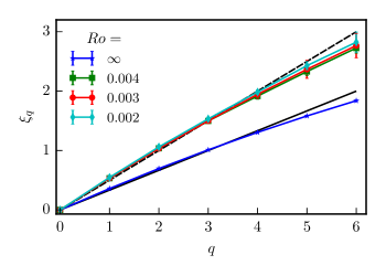
Figure 3: The scaling exponents $\xi_{q}$ (with error bars and connected by lines as a guide to the eye), from our shell model simulations, of the equal-time structure function for different Rossby numbers (see Table I and, for comparison with direct numerical simulations, Table II), including the case of no rotation ($Ro=\infty$). For finite values of rotation, the exponents differ significantly from those obtained for non-rotating turbulence as well (lower set of data points, in blue, with the Kolmogorov scaling $q/3$ shown by a black solid line) as the dimensional prediction $\xi=q/2$ (black dashed line) for rotating flows. Nevertheless as $Ro\ll 1$, the exponents seem to asymptote to the dimensional prediction suggesting a suppression of intermittency in the flow and consequently a loss of multiscaling.

In order to get a sense of how close the structure functions are to the dimensional prediction $S_{q}(k_{n})\sim k_{n}^{-q/2}$ (as $Ro\to 0$), we first adopt a strategy similar to that used more traditionally for the energy spectrum (Fig. 1), namely to look at plots of the compensated structure function $k_{n}^{q/2}S_{q}(k_{n})$ for a sufficiently small value of the Rossby number. In Fig. 2, we plot these compensated structure functions for several orders for $Ro=0.002$. The shading region marks the inertial range of scales smaller than the Zeman wavenumber. These plots suggest that there is a clear departure from the dimensional prediction, especially for higher orders, due to the familiar intermittency corrections. Indeed, in the inset of the same figure and for the same Rossby number, we plot the flatness $S_{4}/S_{2}^{2}$ as a function of the wavenumber to illustrate more clearly the issue of scale-by-scale intermittency for such systems.

All of these suggests that it is vital now to make our observations more quantitative by actually measuring the equal-time exponents for different values of the Rossby number. As is common to such measurements, we use the extended-self-similarity (ESS) procedure to extract more reliable estimates of the scaling exponents Benzi et al. (1993); Chakraborty, Frisch, and Ray (2010); Chakraborty et al. (2012). Furthermore, given the spacing of wavenumbers in a shell model a local slope analysis, a natural choice for data from direct numerical simulations, is not as useful. We therefore use a different statistical measure of the errors on our measurement. We obtain $S_{q}(k_{n})$, and thus $\xi_{q}$, after averaging over several large eddy turn over times. We then repeat this for 49 other statistically independent measurements to obtain 50 statistically independent measurements of $\xi_{q}$. The mean of these yield the final exponents that we quote and their standard deviations become our error bars.

In Fig. 3, we plot the equal-time scaling exponents $\xi_{q}$ as a function of $q$ (also listed in Table I for different (small) values of $Ro$), from our shell model simulations, for different strengths of the Coriolis force. For comparison, we also show the exponents $\xi_{q}$ for non-rotation turbulence ($\Omega=0;Ro=\infty$) and the associated black solid line indicating the $q/3$ prediction of Kolmogorov. The black dashed line corresponds to the dimensional prediction $q/2$ and our measurements clearly show $\xi_{q}\neq q/2$, with the effect becoming more pronounced Baroud et al. (2002, 2003) for $q>3$. For rotating flows, we of course present results in Fig. 3 for sufficiently low Rossby numbers. This is because for weak rotation (large Rossby numbers), the Zeman wavenumber is small leading to a shrinking inertial range (see Fig. 1) not amenable to the extraction of higher order scaling exponents. Hence, we do not show the exponents for such high Rossby numbers in Fig. 3. However, as $Ro\to 0$, the scaling exponents tend to asymptote to values more consistent with the dimensional prediction showing a strong depletion of intermittency effects. This behaviour has been noted in earlier studies Müller and Thiele (2007); Seiwert, Morize, and Moisy (2008); Mininni, Alexakis, and Pouquet (2009) that showed that strong rotation leads to a depletion of intermittency effects in turbulent flows. What is intriguing is that this feature is faithfully reproduced in a low-dimensional dynamical system—shell model—which is insensitive to any geometrical effects and the proliferation of columnar vortices in real flows or solutions of the Navier–Stokes equation. Furthermore, the exponents from our shell model simulations (Fig. 3 and Table I) are in agreement with those reported, for similar Rossby numbers, from direct numerical simulations of earlier studies, such as the work of Thiele and Müller Thiele and Müller (2009) (see Table II). We note, in passing, that measurements of equal-time exponents for wavenumbers $k>k_{\Omega}$ (but smaller than the dissipation range) yield exponents which are consistent with what is known for non-rotating, homogeneous and isotropic, three-dimensional turbulence.

IV Energy Dissipation Rate

The three-dimensional Navier–Stokes equation is known to be invariant under suitable scaling transformations Frisch (1995) with a scaling exponent $h$ which allows us to write the (scalar) velocity increments $\delta u_{r}$ across a scale $r$ as $\delta u_{r}\sim r^{h}$. Phenomenologically, the scale-dependent mean kinetic energy dissipation rate $\epsilon(r)\sim\frac{\delta u_{r}^{3}}{r}\sim r^{\alpha-1}$, where $\alpha=3h$. For homogeneous and isotropic turbulence, Kolmogorov theory, in the absence of intermittency or multifractal statistics, predicts $h=1/3$ which ensures, in the inertial range, a scale-independent dissipation rate equal to the constant energy flux across these scales. Real turbulence, though, is multifractal. Thus the dissipation field cannot be characterized by a unique choice of $\alpha$ but rather by its singularity spectrum $f(\alpha)$ and the mass function of Renyi dimension $\tau(q)$, both of which we define precisely later.

In a three-dimensional flow the local energy dissipation rate

$$\varepsilon(\mathbf{x})=\frac{\nu}{2}\sum_{i,j}(\partial_{i}u_{j}+\partial_{j}u_{i})^{2},$$ (5)

is a function of all three spatial directions. For shell models, given its lack of spatial structure, obtaining the analogue of such a scalar dissipation field amenable to a multifractal analysis is less obvious. Let us nevertheless assume that the shell model describes the flow in a spatial domain of size $L$ and that the energy dissipation rate can be defined at any spatial position $x\in[0,L]$. Thus, keeping in mind the Richardson picture of energy cascade, it is natural to assume that beginning with the largest eddy of size $\sim L$, an energy cascade is set up in the system such that each eddy in a given generation $m$ of the cascade breaks up into 2 to provide the eddies of the next generation. This suggests a hierarchical transfer of energy, scale-by-scale, such that at each scale $m\in\{0,1,2,\cdots,K\}$, the number of eddies is $2^{m}$ and the typical size of each eddy is $l_{m}=L/2^{m}\sim 1/k_{m}$ (since the wave-numbers in a shell model correspond to the inverse of the spatial scales). The smallest scales, set by $K$, correspond to the viscosity-dominated Kolmogorov scale of the flow. Let us now focus on the $i$-th eddy (of size $l_{m}=L/2^{m}\sim 1/k_{m}$) out of the $2^{m}$ eddies of generation $m$. Denoting the energy of this eddy by $E_{i}^{(m)}$, the total energy at scale $l_{m}$ must correspond to the kinetic-energy of the $m$-th shell in our shell model: $|u_{m}|^{2}\equiv 2\sum_{i=1}^{2^{m}}E_{i}^{(m)}$ with an associated energy density $E_{i}^{(m)}/l_{m}$ in the $i$-th eddy. Thus we adapt the multifractal cascade ideas of Meneveau and Sreenivasan Meneveau and Sreenivasan (1987a) and construct it for our shell model. Furthermore, we choose different fractions $p\in(0.5,0.9]$ of the energy distribution amongst the daughter eddies and find that our results are qualitatively insensitive to the particular choice of $p$; in this paper we report results for $p=0.7$.

With these definitions, following Lepreti et al. Lepreti, Carbone, and Veltri (2006), the kinetic energy density $e(x)$ at a spatial location $x\in[0,L]$ is given by the contributions from eddies of all scales which have their imprints on a specific point $x$: $e(x)=\sum_{m=0}^{K}E_{s_{m}(x)}^{(m)}/l_{m}$ where $s_{m}(x):=\lceil(x-1)/l_{m}\rceil$ and thence the one-dimensional energy dissipation rate

$$\varepsilon(x)=2\nu\sum_{m=0}^{K}k_{m}^{2}E_{s_{m}(x)}^{(m)}/l_{m}$$ (6)

in the shell model. We refer to the reader to Lepreti et al. (2006) Lepreti, Carbone, and Veltri (2006) for a detailed description on how $\epsilon(x)$ is evaluated in the shell model at any given instant of time from the knowledge of the energy content of the eddies in the previous time step. In our calculations, we choose the largest length scale $L$ as the one associated with the forcing shell, i.e., $n=3$, and ${K}=23$ to obtain a grid resolution $L/2^{20}$. Finally, to obtain reliable statistics, we extract the spatial distribution $\epsilon(x)$ from 100 different, statistically-independent velocity configurations in the steady state.

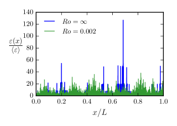
Figure 4: Reconstructed cuts of the energy dissipation rate following Lepreti et al. Lepreti, Carbone, and Veltri (2006) (see text) from our simulations of the helical shell model. It suggests a suppression of intermittency when the flow is strongly rotating.

In Fig. 4, we show a representative plot of $\varepsilon(x)$, obtained from our shell model data as described above, for the case of the non-rotating flow and one with $Ro=0.002$. Fig. 4 suggests that the behaviour of a spatial trace of the energy dissipation rate, at any given instant in time, obtained from the low-dimensional model is consistent with what is seen in direct numerical simulations of such flows (see also Fig. 7 in Appendix A, obtained from our DNS). It is clear though that given the much higher Reynolds number that our shell model achieves (as well as the more intermittent nature of such cascade models), the intensity of the intermittent peaks in the dissipation rate in Fig 4 are much stronger than what is seen in DNSs. Furthermore, when we compare the cuts of these dissipation rates for the rotating and non-rotating cases, we do see a suggestion—the relatively calmer traces of $\varepsilon$—that intermittency is suppressed (along with the degree of multifractality) as soon as we have a small enough Rossby number. However, this visual evidence is hardly compelling and in order to substantiate our claim, we must resort to a more quantitative characterization of this phenomenon through a full multifractal analysis.

V Multifractal Analysis

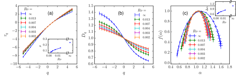
Figure 5: Signatures of decreasing intermittency with increased rotation. The figure depicts (a) the Rényi scaling exponents $\tau_{q}$ (inset: the intermittency exponent $\mu$ as a function of $Ro$), (b) the generalised dimension $D_{q}$, and (c) the singularity spectrum $f(\alpha)$ (inset: widths $\Delta\alpha$ as a function of $Ro$), for different values of $Ro$, of the energy dissipation obtained from our simulations of the helical shell model and with $p=0.7$ (see text).

We set the stage for this analysis by defining, through the 1D cuts of the dissipation field $\varepsilon(x)$, a scale-dependent energy dissipation $\varepsilon_{r}\equiv\int_{x\in I_{r}}\varepsilon(x)dx$ integrated in an interval $I_{r}$ of size $r$. If we choose the interval all the way up to the integral scale $L$, this gives a reference scale-dependent dissipation $\varepsilon_{L}$ which allows us to define the Rényi scaling exponent $\tau_{q}$ via

$$\langle\epsilon_{r}^{q}\rangle\sim\epsilon_{L}^{q}\left(\frac{r}{L}\right)^{\tau_{q}}$$ (7)

for $L\gg r\gg\eta$. By using this exponent $\tau_{q}$, we can define the generalised dimension Hentschel and Procaccia (1983) $D_{q}=\tau_{q}/(q-1)$ and the multifractal singularity spectrum Halsey et al. (1986); Ott (2002) through a Legendre transform of $\tau_{q}$ as $f(\alpha)=\min_{q}(q\alpha-\tau_{q})$ where $\alpha={d\tau_{q}}/{dq}$. As is traditional in this field, we characterize intermittency Meneveau and Sreenivasan (1991) through the exponent $\mu=-({d^{2}\tau_{q}}/{dq^{2}})_{q=0}$ ($\mu\approx 0.26$ for the non-rotating case) and the width of the singularity spectrum $\Delta\alpha=\alpha_{\rm max}-\alpha_{\rm min}$, where $\alpha_{\rm min}$ and $\alpha_{\rm max}$ are the strongest and weakest singularities, respectively: Self-similar solutions are naturally characterised by $\Delta\alpha=0$ and $q$-independent generalised dimension.

From our simulations of the helical shell model we first calculate $\tau_{q}$ via Eq. 7, directly Hentschel and Procaccia (1983); Halsey et al. (1986) from the statistics of dissipation and from there the generalised dimension $D_{q}$ as well as the intermittency exponent $\mu$. The singularity spectrum $f(\alpha)$ is obtained independently using the method proposed by Chhabra and Jensen Chhabra and Jensen (1989); Chhabra et al. (1989); we have confirmed that a numerical calculation of $f(\alpha)$ from $D_{q}$ by using the Legendre transform yields similar results but with larger error bars. In practice, we choose a long time series for the dissipation rate (Fig. 4) from which we are able to compute $\tau_{q}$ for $q\in[-5,5]$. Such a large range of $q$ is important to ensure that the the generalised dimensions (computed through $\tau_{q}$) and the singularity spectrum shows definite signs of convergence: Namely, $D_{q}$ reaching a plateau for the largest $|q|$ with an associated infinite slope of the singularity spectrum for the largest and smallest measured $\alpha$ (which corresponds to the extremal values of $D_{q}$ as $q\to-\infty$ and $q\to\infty$, respectively). Finally, we calculate $D_{q}$, $f(\alpha)$, and $\tau_{q}$ (and thus the intermittency exponent $\mu$), from several independent runs; in Fig. 5 we plot the means of these measurements and show their standard deviations as error bars.

In panel (a) of Fig. 5 we show plots of $\tau_{q}$ as a function of $q$ for different strengths of rotations. We notice, visually, a diminishing of the curvature of $\tau_{q}$ around $q=0$ suggesting a depletion of intermittency. This is confirmed by measuring $\mu$ for different values of $Ro$ (inset, Fig. 5(a)); as $Ro\to 0$, there is a significant decrease in $\mu$ compared to the $Ro=\infty$ (non-rotating) value for homogeneous and isotropic turbulence. This observations if further strengthened by looking at plots of $D_{q}$ vs. $q$ in Fig. 5(b) which plateau (as $|q|\gg 1$) to values much closer to 1 as the Rossby numbers decrease. This is confirmed in in panel (c) where we show the singularity spectrum $f(\alpha)$ and the widths $\Delta\alpha$ as insets. With increasing rotation, the spectrum narrows, quantified by $\Delta\alpha$ which shows a monotonic decrease with $Ro$.

Thus our multifractal analysis on the shell model data strongly suggests that the lack of self-similarity (and intermittent behaviour) in the statistics of the dissipation rate—as measured through the generalised dimension $D_{q}$, the singularity spectrum $f(\alpha)$ and the exponent $\tau_{q}$—weakens considerably with increasing strengths of rotation. Indeed in the limit $Ro\to 0$, it may be argued that the dissipation range statistics may well recover a truly self-similar form which would be consistent with the dimensional (non-intermittent) prediction of the inertial range (anomalous) scaling exponent $\xi_{q}$.

All of this then naturally brings us to an important question: For rotating turbulence (especially in the limit $Ro\ll 1$), is there a way to bridge the statistics of the dissipation rates, characterised by generalised dimension $D_{q}$ with the (anomalous) inertial range scaling exponents $\xi_{q}$? In other words, what would be the analogue of the familiar $\zeta_{q}=q/3+(q/3-1)(D_{q/3}-1)$ result Meneveau and Sreenivasan (1987b) for non-rotating, homogeneous and isotropic turbulence?

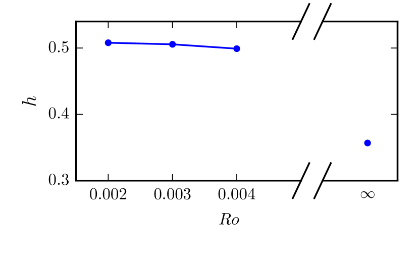
Figure 6: The scaling exponent $h$ versus the Rossby number $Ro$ from our shell model simulations. The exponent saturates to $h=1/2$ in the strong rotation limit $Ro\ll 1$ and to $h=1/3$ in the case of no rotation $Ro=\infty$.

To answer this question, we make the following ansatz when $Ro\neq\infty$:

$$\xi_{q}=hq+(hq-1)(D_{hq}-1)$$ (8)

which can be re-arranged in the more useful form (for what is to follow):

$$\frac{\xi_{q}-1}{D_{hq}}+1=hq.$$ (9)

(For $Ro=\infty$ or $\Omega=0$, the scaling exponent $h=1/3$.)

By using our measurements of the scaling exponents $\xi_{q}$ and $D_{q}$, we use Eq. (9) to obtain the scaling exponent $h$ as a function of $Ro$; our results are shown in Fig. 6. Indeed, as we would expect from phenomenology (and also consistent with Fig. 1), as $Ro\to 0$, the exponent $h\to 1/2$ while, in for the case of no rotation ($Ro=\infty$), $h=1/3$. This leads us to conjecture, in the limit $Ro\to 0$, the following relation bridging the dissipation range and the inertial range statistics:

$$\xi_{q}=q/2+(q/2-1)(D_{q/2}-1);\quad\quad Ro\to 0.$$ (10)

Furthermore, this relationship shows how the emergence of an approximate self-similarity ($\Delta\alpha\to 0$ and a $q$-independent generalised dimension) as $Ro\to 0$, leads to a progressively simple scaling (and not multi-scaling) of the exponents of the equal-time structure functions as shown in Fig. 3. It is worth emphasizing that, in the limit $Ro\rightarrow 0$, the Zeman scale is pushed all the way up to the dissipation scale as indicated in Fig. 1 making the K41 ($k^{-5/3}$) scaling no longer discernible: The $k^{-2}$ spectral scaling dominates all the way up to the dissipation scale. It is in this limit, of course, that our relation (10) holds.

$Ro$	$q$	$\xi_{q}$	$q/2+(q/2-1)(D_{q/2}-1)$
	1	0.513 $\pm$ 0.007	0.513 $\pm$ 0.001
	2	1	1.0 $\pm$ 0.0
0.004	3	1.44 $\pm$ 0.03	1.463 $\pm$ 0.003
	4	1.85 $\pm$ 0.05	1.905 $\pm$ 0.007
	5	2.25 $\pm$ 0.07	2.31 $\pm$ 0.01
	6	2.63 $\pm$ 0.09	2.70 $\pm$ 0.02
	1	0.516 $\pm$ 0.004	0.512 $\pm$ 0.002
	2	1	1.0 $\pm$ 0.0
0.003	3	1.45 $\pm$ 0.03	1.469 $\pm$ 0.004
	4	1.88 $\pm$ 0.07	1.92 $\pm$ 0.01
	5	2.3 $\pm$ 0.1	2.35 $\pm$ 0.02
	6	2.7 $\pm$ 0.2	2.77 $\pm$ 0.03
	1	0.516 $\pm$ 0.008	0.510 $\pm$ 0.001
	2	1	1.0 $\pm$ 0.0
0.002	3	1.45 $\pm$ 0.03	1.471 $\pm$ 0.003
	4	1.87 $\pm$ 0.04	1.913 $\pm$ 0.007
	5	2.29 $\pm$ 0.07	2.35 $\pm$ 0.01
	6	2.7 $\pm$ 0.2	2.78 $\pm$ 0.02

Table 1: Summary of results from simulations of our shell model for different Rossby numbers. The excellent agreement between columns 3 ($\xi_{q}$, the left hand side of Eq. (10)) and 4 ($q/2+(q/2-1)(D_{q/2}-1)$, the right hand side of Eq. (10)) is evidence for the central theoretical prediction of this work.

Our theoretical prediction, while similar in spirit to earlier results of the homogeneous and isotropic turbulence, still needs an independent check from numerical data. A convincing way to do this is to independently evaluate the left-hand-side ($\xi_{q}$, corresponding to inertial range statistics) and the right-hand-side ($q/2+(q/2-1)(D_{q/2}-1)$, corresponding to dissipation range statistics) of Eq. (10) from our simulations of the shell model and check if the equality holds for sufficiently small values of $Ro$ and several values of $q$. Given that we have already calculated the equal-time exponents $\xi_{q}$ (Fig. 3) and the generalised dimensions $D_{q}$ (Fig. 5(b)) for different values of $q$, it is straightforward now to carry out this validation. In Table I, we show values of the left-hand-side (column 3) right-hand-side (column 4) of Eq. (10) for $q=1,2,...,6$; furthermore we present results for 3 different, but sufficiently small, values of $Ro$. A comparison of columns 3 and 4, for any given $q$ (and $Ro$), leaves little doubt as to the validity of our prediction bridging the inertial range and the dissipation range statistics.

$Ro$	$q$	$\xi_{q}$	$q/2+(q/2-1)(D_{q/2}-1)$
	1	0.52 $\pm$ 0.003	0.528 $\pm$ 0.006
	2	1	1.0 $\pm$ 0.0
0.005	3	1.43 $\pm$ 0.006	1.42 $\pm$ 0.02
	4	1.82 $\pm$ 0.02	1.80 $\pm$ 0.04
	5	2.15 $\pm$ 0.03	2.13 $\pm$ 0.08
	6	2.42 $\pm$ 0.05	2.4 $\pm$ 0.1
	1	0.52 $\pm$ 0.002	0.522 $\pm$ 0.005
	2	1	1.0 $\pm$ 0.0
0.001	3	1.43 $\pm$ 0.007	1.43 $\pm$ 0.01
	4	1.80 $\pm$ 0.02	1.82 $\pm$ 0.02
	5	2.13 $\pm$ 0.03	2.17 $\pm$ 0.04
	6	2.42 $\pm$ 0.05	2.48 $\pm$ 0.05

Table 2: A summary of results from direct numerical simulations confirming the validity of Eq. (10) for two different values of the Rossby number (column 1). The equal-time exponents $\xi_{q}$ (column 3) for the plane perpendicular to the axis of rotation, are those reported, from the DNS studies by Thiele and Müller Thiele and Müller (2009); the generalised dimension $D_{q}$ (column 4) are from our dissipation rate statistics for the plane perpendicular to the axis of rotation (Fig. 7a). The excellent agreement between columns 3 and 4 is compelling evidence for the validity of Eq. (10).

Before we conclude, it is tempting to validate Eq. (10) against data from actual direct numerical simulations. Although DNSs are not the central focus of this study, such an exercise is useful in this case for the sake of completeness. We use data for the equal-time exponents of the axis-perpendicular longitudinal velocity structure functions from the work of Thiele and Müller Thiele and Müller (2009) who used similarly small values of Rossby numbers. However in order to compute the generalised dimensions $D_{q}$ and thence the right-hand-side of Eq. (10), we perform DNSs (see Appendix A for details) corresponding to the Rossby numbers used by Thiele and Müller Thiele and Müller (2009). In a manner exactly similar to Table I, we show, in Table II, the left-hand-side and right-hand-side of our bridge relation by using data from DNSs. Once again, a comparison of columns 3 and 4 suggests clearly for small enough Rossby numbers, it is indeed possible to bridge the statistics of the inertial and the dissipation ranges.

VI Conclusion

Equation (10) captures the key result in this study by bridging, in the limit of strongly rotating ($Ro\to 0$) turbulence, the statistics of the energy dissipation rate characterised by the generalised dimension $D_{q}$ with the scaling exponents $\xi_{q}$ of the moments of velocity increments over scales $r$ in the inertial range. Furthermore our analysis provides a more complete description of the depletion of intermittency in flows affected strongly by the Coriolis force. Furthermore, our work shows that even for anisotropic system such as rotating turbulence, shell models, while being insensitive to the spatial reorganisation of the flow due to the Coriolis force, are nevertheless able to capture the scaling laws of two-point correlation functions in a way consistent with direct numerical simulations. Indeed, our work shows that following Lepreti et al. Lepreti, Carbone, and Veltri (2006) (see also Meneveau et al. Meneveau and Sreenivasan (1987a)), it is possible to extract a spatial profile of the dissipation rates in such shell models that can be used for future studies of the small-scale statistics of different forms of turbulence for whom such a low-dimensional dynamical systems representation exists. In this context, it is worth mentioning that there is another useful method Jensen (1999); Roux and Jensen (2004); Chakraborty, Jensen, and Sarkar (2010); Chakraborty, Jensen, and Madsen (2010) of generating a synthetic real space velocity field from the shell models; it could provide complementary insights in such studies.

Finally, we remind ourselves that this paper studies the problem of bridging inertial and dissipative statistics in the limit where the mean helicity vanishes. Although we have some evidence that for small values of the mean helicity our results and conclusions are unaltered, it would be important to study in future the problem of non-zero helicity and how it should modify the central result captured in Eq. (10); the helical shell model used in this paper is particularly useful from this point of view as it allows us to introduce a mean helicity in a controlled way. Furthermore, Eq. (10) is an asymptotic result valid in the vanishing Rossby number limit; we leave for future work possible Rossby number corrections to this prediction.

Data Availability

The data that support the findings of this study are available from the corresponding author on request.

Appendix A Direct Numerical Simulations

Our direct numerical simulations, which were performed to provide additional support for our theoretical predictions, were performed with a standard fully de-aliased pseudo-spectral method to solve Eq. (1) on a $2\pi$ periodic cubic box, with $N^{3}=512^{3}$ collocation points, and a fourth-order Runge-Kutta scheme for time-marching. In our simulations, an adaptive time-step $\delta t$ consistent with the Courant–Friedrich–Lewy (CFL) condition is employed and the viscosity $\nu=10^{-3}$ is chosen to obtain Taylor-scale based Reynolds numbers $Re_{\lambda}=50$ and $58$, corresponding to rotation rates $\Omega=8$ and $32$ (or equivalently, $Ro=0.005$ and $0.001$), respectively. As is the case in the simulations of our shell model, we use a forcing

$$\mathbf{{f}}(\mathbf{k})=\frac{\epsilon{\mathbf{u}}(\mathbf{k})}{n_{f}\left[{\mathbf{u}}(\mathbf{k})\cdot{\mathbf{u}}^{*}(\mathbf{k})\right]},$$ (11)

which allows for a constant-energy injection (and no kinetic-helicity) at wavenumber $\mathbf{k}_{f}\in[{40,41}]$ ($n_{f}$ is the number of modes at this wavenumber) to drives the system to a statistically stationary, isotropic and homogeneous, turbulent regime. Once we reach such a stationary state, we turn on the Coriolis force. We then wait a sufficiently long time for the rotating system to reach a statistically stationary state before measuring the local energy dissipation rates (Figs. 7(a) and (b)) and from there the generalised dimension $D_{q}$ necessary for the verification of Eq.(10) (see Table II).

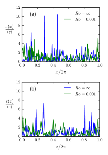
Figure 7: Representative snapshots of the one-dimensional cuts of the energy dissipation rates from our DNSs along the (a) x-axis and (b) z-axis. A comparison of the panels with Fig. 4 show qualitatively similar features with a more intermittent—higher peaks—behaviour in the data from our shell model consistent with its much larger Reynolds number. These plots also suggest a suppression of intermittency when the flow is strongly rotating.

A convenient way to carry out a multifractal analysis of energy dissipation field is to take several one-dimensional (1D) cuts of $\varepsilon(\mathbf{x})$ parallel and perpendicular to the direction of rotation ($z-$axis). These 1D cuts along the axis of rotation yield $\varepsilon(z)=\varepsilon(x_{0},y_{0},z)$; similarly, for the plane perpendicular to the axis of rotation, we obtain $\varepsilon(x)=\varepsilon(x,y_{0},z_{0})$ and $\varepsilon(y)=\varepsilon(x_{0},y,z_{0})$. For reliable statistics, we choose 49 cuts along each direction with different values of $x_{0}$, $y_{0}$ and $z_{0}$ lying in the interval $[\pi/4,3\pi/4]$. Considering that the data size for a cut is small, we employ a waveletMeneveau (1991) leaders based method Jaffard, Lashermes, and Abry (2007); Wendt and Abry (2007) to calculate the Rényi scaling exponents, and thence the generalized dimensions.

In Figs. 7(a) and (b) we show representative plots of one such cut for the reconstructed $\varepsilon(x)$ and $\varepsilon(z)$, respectively, normalised by the global mean, at a single instant of time for the non-rotating case and one with Rossby number $Ro=0.001$ which illustrates that highly intermittent nature of the dissipation field persists even for such 1D cuts. It is worth remarking that such fields are strikingly similar (with less extreme excursions) to the ones reported in the paper from our shell model simulations. Finally, we mention in passing, that the singularity spectrum $f(\alpha)$ and the exponent $\tau_{q}$ from these DNSs are in excellent agreement to those reported in this paper from our shell model study.

Our DNSs were performed by using the open-source code “Tarang” Verma et al. (2013); Chatterjee et al. (2018) developed at IIT Kanpur.

References

References

- Frisch (1995) U. Frisch, Turbulence: The Legacy of A. N. Kolmogorov (Cambridge University Press, 1995).
- Lohse and Grossmann (1993) D. Lohse and S. Grossmann, “Intermittency in turbulence,” Physica A: Statistical Mechanics and its Applications 194, 519–531 (1993).
- Kolmogorov (1941a) A. N. Kolmogorov, “The local structure of turbulence in incompressible viscous fluid for very large Reynolds numbers,” Dokl. Akad. Nauk SSSR 30, 301–305 (1941a).
- Kolmogorov (1941b) A. N. Kolmogorov, “Dissipation of energy in locally isotropic turbulence,” Dokl. Akad. Nauk SSSR 32, 16–18 (1941b).
- Kolmogorov (1962) A. N. Kolmogorov, “A refinement of previous hypotheses concerning the local structure of turbulence in a viscous incompressible fluid at high reynolds number,” Journal of Fluid Mechanics 13, 82–85 (1962).
- Kailasnath, Sreenivasan, and Stolovitzky (1992) P. Kailasnath, K. Sreenivasan, and G. Stolovitzky, “Probability density of velocity increments in turbulent flows,” Phys. Rev. Lett. 68, 2766–2769 (1992).
- La Porta et al. (2001) A. La Porta, G. A. Voth, A. M. Crawford, J. Alexander, and E. Bodenschatz, “Fluid particle accelerations in fully developed turbulence,” Nature 409, 1017–1019 (2001).
- Batchelor and Townsend (1949) G. K. Batchelor and A. A. Townsend, “The nature of turbulent motion at large wave-numbers,” Proceedings of the Royal Society of London. Series A. Mathematical and Physical Sciences 199, 238–255 (1949).
- Siggia (1981) E. D. Siggia, “Numerical study of small-scale intermittency in three-dimensional turbulence,” Journal of Fluid Mechanics 107, 375 (1981).
- Mandelbrot (1972) B. B. Mandelbrot, “Possible refinement of the lognormal hypothesis concerning the distribution of energy dissipation in intermittent turbulence,” in Statistical Models and Turbulence (Springer Berlin Heidelberg, 1972) pp. 333–351.
- Kraichnan (1974) R. H. Kraichnan, “On kolmogorov’s inertial-range theories,” Journal of Fluid Mechanics 62, 305 (1974).
- Mandelbrot (1974) B. B. Mandelbrot, “Intermittent turbulence in self-similar cascades: divergence of high moments and dimension of the carrier,” Journal of Fluid Mechanics 62, 331–358 (1974).
- Frisch, Sulem, and Nelkin (1978) U. Frisch, P.-L. Sulem, and M. Nelkin, “A simple dynamical model of intermittent fully developed turbulence,” Journal of Fluid Mechanics 87, 719–736 (1978).
- Frisch and Parisi (1985) U. Frisch and G. Parisi, “Turbulence and predictability in geophysical fluid dynamics and climate dynamics,” (North-Holland Publ. Co., Amsterdam/New York, 1985) Chap. On the singularity structure of fully developed turbulence, p. 84.
- Pandit, Perlekar, and Ray (2009) R. Pandit, P. Perlekar, and S. S. Ray, “Statistical properties of turbulence: An overview,” Pramana 73, 157 (2009).
- Greenspan (1968) Greenspan, The Theory of Rotating Fluids (Cambridge University Press, 1968).
- Moffatt (1983) H. K. Moffatt, “Transport effects associated with turbulence with particular attention to the influence of helicity,” Rep. Prog. Phys. 46, 621 (1983).
- Davidson (2013) P. A. Davidson, Turbulence in Rotating, Stratified and Electrically Conducting Fluids (Cambridge University Press, 2013).
- Barnes (2001) S. A. Barnes, “An assessment of the rotation rates of the host stars of extrasolar planets,” Astrophys. J. 561, 1095–1106 (2001).
- Cho et al. (2008) J. Y.-K. Cho, K. Menou, B. M. S. Hansen, and S. Seager, “Atmospheric circulation of close-in extrasolar giant planets. i. global, barotropic, adiabatic simulations,” Astrophysic. J. 675, 817 (2008).
- Le Reun et al. (2017) T. Le Reun, B. Favier, A. J. Barker, and M. Le Bars, “Inertial wave turbulence driven by elliptical instability,” Phys. Rev. Lett. 119, 034502 (2017).
- Aurnou et al. (2015) J. Aurnou, M. Calkins, J. Cheng, K. Julien, E. King, D. Nieves, K. Soderlund, and S. Stellmach, “Rotating convective turbulence in earth and planetary cores,” Physics of the Earth and Planetary Interiors 246, 52 – 71 (2015).
- Smith and Waleffe (1999) L. M. Smith and F. Waleffe, “Transfer of energy to two-dimensional large scales in forced, rotating three-dimensional turbulence,” Phys. Fluids 11, 1608–1622 (1999).
- Müller and Thiele (2007) W.-C. Müller and M. Thiele, “Scaling and energy transfer in rotating turbulence,” EPL (Europhysics Letters) 77, 34003 (2007).
- Mininni, Alexakis, and Pouquet (2009) P. D. Mininni, A. Alexakis, and A. Pouquet, “Scale interactions and scaling laws in rotating flows at moderate rossby numbers and large reynolds numbers,” Physics of Fluids 21, 015108 (2009).
- Bartello (1995) P. Bartello, “Geostrophic adjustment and inverse cascades in rotating stratified turbulence,” Journal of the Atmospheric Sciences 52, 4410–4428 (1995).
- Métais et al. (1996) O. Métais, P. Bartello, E. Garnier, J. Riley, and M. Lesieur, “Inverse cascade in stably stratified rotating turbulence,” Dynamics of Atmospheres and Oceans 23, 193 – 203 (1996), stratified flows.
- Yarom, Vardi, and Sharon (2013) E. Yarom, Y. Vardi, and E. Sharon, “Experimental quantification of inverse energy cascade in deep rotating turbulence,” Physics of Fluids 25, 085105 (2013).
- Bartello, Métais, and Lesieur (1994) P. Bartello, O. Métais, and M. Lesieur, “Coherent structures in rotating three-dimensional turbulence,” Journal of Fluid Mechanics 273, 1–29 (1994).
- Godeferd and Lollini (1999) F. S. Godeferd and L. Lollini, “Direct numerical simulations of turbulence with confinement and rotation,” J. Fluid Mech. 393, 257–308 (1999).
- Zeman (1994) O. Zeman, “A note on the spectra and decay of rotating homogeneous turbulence,” Physics of Fluids 6, 3221–3223 (1994).
- Hattori, Rubinstein, and Ishizawa (2004) Y. Hattori, R. Rubinstein, and A. Ishizawa, “Shell model for rotating turbulence,” Physical Review E 70 (2004).
- Sreenivasan and Davidson (2008) B. Sreenivasan and P. A. Davidson, “On the formation of cyclones and anticyclones in a rotating fluid,” Phys. Fluids 20, 085104 (2008).
- Pouquet and Mininni (2010) A. Pouquet and P. D. Mininni, “The interplay between helicity and rotation in turbulence: implications for scaling laws and small-scale dynamics,” Philos. Trans. R. Soc. Lond., A 368, 1635–1662 (2010).
- Castello and Clercx (2011) L. D. Castello and H. J. H. Clercx, “Lagrangian velocity and acceleration auto-correlations in rotating turbulence,” Journal of Physics: Conference Series 318, 052028 (2011).
- Biferale et al. (2016) L. Biferale, F. Bonaccorso, I. Mazzitelli, M. van Hinsberg, A. Lanotte, S. Musacchio, P. Perlekar, and F. Toschi, “Coherent structures and extreme events in rotating multiphase turbulent flows,” Physical Review X 6 (2016).
- Maity, Govindarajan, and Ray (2019) P. Maity, R. Govindarajan, and S. S. Ray, “Statistics of lagrangian trajectories in a rotating turbulent flow,” Phys. Rev. E 100, 043110 (2019).
- Ibbetson and Tritton (1975) A. Ibbetson and D. J. Tritton, “Experiments on turbulence in a rotating fluid,” J.Fluid Mech. 68, 639–672 (1975).
- Hopfinger, Browand, and Gagne (1982) E. J. Hopfinger, F. K. Browand, and Y. Gagne, “Turbulence and waves in a rotating tank,” J. Fluid. Mech. 125, 505–534 (1982).
- Bewley et al. (2007) G. P. Bewley, D. P. Lathrop, L. R. M. Maas, and K. R. Sreenivasan, “Inertial waves in rotating grid turbulence,” Physics of Fluids 19, 071701 (2007).
- Morize, Moisy, and Rabaud (2005) C. Morize, F. Moisy, and M. Rabaud, “Decaying grid-generated turbulence in a rotating tank,” Phys. Fluids 17, 095105 (2005).
- Moisy et al. (2011) F. Moisy, C. Morize, M. Rabaud, and J. Sommeria, “Decay laws, anisotropy and cyclone–anticyclone asymmetry in decaying rotating turbulence,” Journal of Fluid Mechanics 666, 5–35 (2011).
- Yarom, Salhov, and Sharon (2017) E. Yarom, A. Salhov, and E. Sharon, “Experimental quantification of nonlinear time scales in inertial wave rotating turbulence,” Phys. Rev. Fluids 2, 122601 (2017).
- Sharma et al. (2018) M. K. Sharma, A. Kumar, M. K. Verma, and S. Chakraborty, “Statistical features of rapidly rotating decaying turbulence: Enstrophy and energy spectra and coherent structures,” Physics of Fluids 30, 045103 (2018).
- Sharma, Verma, and Chakraborty (2018) M. K. Sharma, M. K. Verma, and S. Chakraborty, “On the energy spectrum of rapidly rotating forced turbulence,” Physics of Fluids 30, 115102 (2018).
- Sharma, Verma, and Chakraborty (2019) M. K. Sharma, M. K. Verma, and S. Chakraborty, “Anisotropic energy transfers in rapidly rotating turbulence,” Physics of Fluids 31, 085117 (2019).
- Seiwert, Morize, and Moisy (2008) J. Seiwert, C. Morize, and F. Moisy, “On the decrease of intermittency in decaying rotating turbulence,” Physics of Fluids 20, 071702 (2008).
- Thiele and Müller (2009) M. Thiele and W.-C. Müller, “Structure and decay of rotating homogeneous turbulence,” Journal of Fluid Mechanics 637, 425 (2009).
- Mininni and Pouquet (2010a) P. D. Mininni and A. Pouquet, “Rotating helical turbulence. II. intermittency, scale invariance, and structures,” Physics of Fluids 22, 035106 (2010a).
- Imazio and Mininni (2017) P. R. Imazio and P. D. Mininni, “Passive scalars: Mixing, diffusion, and intermittency in helical and nonhelical rotating turbulence,” Physical Review E 95 (2017).
- Kraichnan (1958) R. H. Kraichnan, “Higher order interactions in homogeneous turbulence theory,” The Physics of Fluids 1, 358–359 (1958).
- Kraichnan (1959) R. H. Kraichnan, “The structure of isotropic turbulence at very high reynolds numbers,” Journal of Fluid Mechanics 5, 497–543 (1959).
- Orszag (1970) S. A. Orszag, “Analytical theories of turbulence,” Journal of Fluid Mechanics 41, 363–386 (1970).
- Lesieur (2008) M. Lesieur, Turbulence in Fluids (Springer, 2008).
- Frisch and Bec (2001) U. Frisch and J. Bec, “Burgulence,” in New trends in turbulence Turbulence: nouveaux aspects: 31 July – 1 September 2000 (Springer Berlin Heidelberg, Berlin, Heidelberg, 2001) pp. 341–383.
- Saha, Chakraborty, and Bhattacharjee (2008) A. Saha, S. Chakraborty, and J. Bhattacharjee, “Dominance of rare events in some problems in statistical physics,” Pramana 71, 413–422 (2008).
- Chakraborty, Saha, and Bhattacharjee (2009) S. Chakraborty, A. Saha, and J. K. Bhattacharjee, “Large deviation theory for coin tossing and turbulence,” Physical Review E 80 (2009).
- Ray (2015) S. S. Ray, “Turbulence in noninteger dimensions by fractal fourier decimation,” Pramana 84, 395 (2015).
- Ray (2018) S. S. Ray, “Non-intermittent turbulence: Lagrangian chaos and irreversibility,” Phys. Rev. Fluids 3, 072601 (2018).
- Lepreti, Carbone, and Veltri (2006) F. Lepreti, V. Carbone, and P. Veltri, “Model for intermittency of energy dissipation in turbulent flows,” Physical Review E 74 (2006).
- Bohr et al. (1998) T. Bohr, M. H. Jensen, G. Paladin, and A. Vulpiani, Dynamical Systems Approach to Turbulence (Cambridge University Press, 1998).
- Biferale (2003) L. Biferale, “Shell models of energy cascade in turbulence,” Annual Review of Fluid Mechanics 35, 441–468 (2003).
- Biskamp (1994) D. Biskamp, “Cascade models for magnetohydrodynamic turbulence,” Phys. Rev. E 50, 2702–2711 (1994).
- Wirth and Biferale (1996) A. Wirth and L. Biferale, “Anomalous scaling in random shell models for passive scalars,” Phys. Rev. E 54, 4982–4989 (1996).
- Basu et al. (1998) A. Basu, A. Sain, S. K. Dhar, and R. Pandit, “Multiscaling in models of magnetohydrodynamic turbulence,” Phys. Rev. Lett. 81, 2687–2690 (1998).
- Frick and Sokoloff (1998) P. Frick and D. Sokoloff, “Cascade and dynamo action in a shell model of magnetohydrodynamic turbulence,” Phys. Rev. E 57, 4155–4164 (1998).
- Mitra and Pandit (2004) D. Mitra and R. Pandit, “Varieties of dynamic multiscaling in fluid turbulence,” Phys. Rev. Lett. 93, 024501 (2004).
- Mitra and Pandit (2005) D. Mitra and R. Pandit, “Dynamics of passive-scalar turbulence,” Phys. Rev. Lett. 95, 144501 (2005).
- Ray, Mitra, and Pandit (2008) S. S. Ray, D. Mitra, and R. Pandit, “The universality of dynamic multiscaling in homogeneous, isotropic navier–stokes and passive-scalar turbulence,” New Journal of Physics 10, 033003 (2008).
- Ray and Basu (2011) S. S. Ray and A. Basu, “Universality of scaling and multiscaling in turbulent symmetric binary fluids,” Phys. Rev. E 84, 036316 (2011).
- Banerjee et al. (2013) D. Banerjee, S. S. Ray, G. Sahoo, and R. Pandit, “Multiscaling in hall-magnetohydrodynamic turbulence: Insights from a shell model,” Phys. Rev. Lett. 111, 174501 (2013).
- Benzi et al. (2003) R. Benzi, E. De Angelis, R. Govindarajan, and I. Procaccia, “Shell model for drag reduction with polymer additives in homogeneous turbulence,” Phys. Rev. E 68, 016308 (2003).
- Kalelkar, Govindarajan, and Pandit (2005) C. Kalelkar, R. Govindarajan, and R. Pandit, “Drag reduction by polymer additives in decaying turbulence,” Phys. Rev. E 72, 017301 (2005).
- Ray and Vincenzi (2016) S. S. Ray and D. Vincenzi, “Elastic turbulence in a shell model of polymer solution,” EPL (Europhysics Letters) 114, 44001 (2016).
- Ditlevsen and Mogensen (1996) P. D. Ditlevsen and I. A. Mogensen, “Cascades and statistical equilibrium in shell models of turbulence,” Phys. Rev. E 53, 4785–4793 (1996).
- Gilbert et al. (2002) T. Gilbert, V. S. L’vov, A. Pomyalov, and I. Procaccia, “Inverse cascade regime in shell models of two-dimensional turbulence,” Phys. Rev. Lett. 89, 074501 (2002).
- Tom and Ray (2017) R. Tom and S. S. Ray, “Revisiting the SABRA model: Statics and dynamics,” EPL (Europhysics Letters) 120, 34002 (2017).
- Chakraborty, Jensen, and Sarkar (2010) S. Chakraborty, M. H. Jensen, and A. Sarkar, “On two-dimensionalization of three-dimensional turbulence in shell models,” The European Physical Journal B 73, 447–453 (2010).
- Benzi et al. (1996) R. Benzi, L. Biferale, R. M. Kerr, and E. Trovatore, “Helical shell models for three-dimensional turbulence,” Physical Review E 53, 3541–3550 (1996).
- Waleffe (1992) F. Waleffe, “The nature of triad interactions in homogeneous turbulence,” Physics of Fluids A: Fluid Dynamics 4, 350–363 (1992).
- Zhou (1995) Y. Zhou, “A phenomenological treatment of rotating turbulence,” Physics of Fluids 7, 2092–2094 (1995).
- Yeung and Zhou (1998) P. K. Yeung and Y. Zhou, “Numerical study of rotating turbulence with external forcing,” Physics of Fluids 10, 2895–2909 (1998).
- Baroud et al. (2002) C. N. Baroud, B. B. Plapp, Z.-S. She, and H. L. Swinney, “Anomalous self-similarity in a turbulent rapidly rotating fluid,” Physical Review Letters 88 (2002).
- Baroud et al. (2003) C. N. Baroud, B. B. Plapp, H. L. Swinney, and Z.-S. She, “Scaling in three-dimensional and quasi-two-dimensional rotating turbulent flows,” Physics of Fluids 15, 2091–2104 (2003).
- Mininni and Pouquet (2010b) P. D. Mininni and A. Pouquet, “Rotating helical turbulence. I. global evolution and spectral behavior,” Physics of Fluids 22, 035105 (2010b).
- Benzi et al. (1993) R. Benzi, S. Ciliberto, R. Tripiccione, C. Baudet, F. Massaioli, and S. Succi, “Extended self-similarity in turbulent flows,” Physical Review E 48, R29–R32 (1993).
- Chakraborty, Frisch, and Ray (2010) S. Chakraborty, U. Frisch, and S. S. Ray, “Extended self-similarity works for the burgers equation and why,” Journal of Fluid Mechanics 649, 275–285 (2010).
- Chakraborty et al. (2012) S. Chakraborty, U. Frisch, W. Pauls, and S. S. Ray, “Nelkin scaling for the burgers equation and the role of high-precision calculations,” Physical Review E 85 (2012).
- Meneveau and Sreenivasan (1987a) C. Meneveau and K. R. Sreenivasan, “Simple multifractal cascade model for fully developed turbulence,” Physical Review Letters 59, 1424–1427 (1987a).
- Hentschel and Procaccia (1983) H. Hentschel and I. Procaccia, “The infinite number of generalized dimensions of fractals and strange attractors,” Physica D: Nonlinear Phenomena 8, 435–444 (1983).
- Halsey et al. (1986) T. C. Halsey, M. H. Jensen, L. P. Kadanoff, I. Procaccia, and B. I. Shraiman, “Fractal measures and their singularities: The characterization of strange sets,” Physical Review A 33, 1141–1151 (1986).
- Ott (2002) E. Ott, Chaos in Dynamical Systems (Cambridge University Press, 2002).
- Meneveau and Sreenivasan (1991) C. Meneveau and K. R. Sreenivasan, “The multifractal nature of turbulent energy dissipation,” Journal of Fluid Mechanics 224, 429 (1991).
- Chhabra and Jensen (1989) A. Chhabra and R. V. Jensen, “Direct determination of the f() singularity spectrum,” Physical Review Letters 62, 1327–1330 (1989).
- Chhabra et al. (1989) A. B. Chhabra, C. Meneveau, R. V. Jensen, and K. R. Sreenivasan, “Direct determination of the f() singularity spectrum and its application to fully developed turbulence,” Physical Review A 40, 5284–5294 (1989).
- Meneveau and Sreenivasan (1987b) C. Meneveau and K. Sreenivasan, “The multifractal spectrum of the dissipation field in turbulent flows,” Nuclear Physics B - Proceedings Supplements 2, 49–76 (1987b).
- Jensen (1999) M. H. Jensen, “Multiscaling and structure functions in turbulence: An alternative approach,” Physical Review Letters 83, 76–79 (1999).
- Roux and Jensen (2004) S. Roux and M. H. Jensen, “Dual multifractal spectra,” Physical Review E 69 (2004).
- Chakraborty, Jensen, and Madsen (2010) S. Chakraborty, M. H. Jensen, and B. S. Madsen, “Three-dimensional turbulent relative dispersion by the gledzer-ohkitani-yamada shell model,” Physical Review E 81 (2010).
- Meneveau (1991) C. Meneveau, “Analysis of turbulence in the orthonormal wavelet representation,” Journal of Fluid Mechanics 232, 469 (1991).
- Jaffard, Lashermes, and Abry (2007) S. Jaffard, B. Lashermes, and P. Abry, “Wavelet leaders in multifractal analysis,” in Wavelet Analysis and Applications, edited by T. Qian, M. I. Vai, and Y. Xu (Birkhäuser Basel, 2007) pp. 201–246.
- Wendt and Abry (2007) H. Wendt and P. Abry, “Multifractality tests using bootstrapped wavelet leaders,” IEEE Transactions on Signal Processing 55, 4811–4820 (2007).
- Verma et al. (2013) M. K. Verma, A. Chatterjee, K. S. Reddy, R. K. Yadav, S. Paul, M. Chandra, and R. Samtaney, “Benchmarking and scaling studies of pseudospectral code tarang for turbulence simulations,” Pramana 81, 617–629 (2013).
- Chatterjee et al. (2018) A. G. Chatterjee, M. K. Verma, A. Kumar, R. Samtaney, B. Hadri, and R. Khurram, “Scaling of a fast fourier transform and a pseudo-spectral fluid solver up to 196608 cores,” Journal of Parallel and Distributed Computing 113, 77–91 (2018).