The frequency of very young galaxies in the local Universe: II. The view from SDSS spectra

Abstract

Only a handful of galaxies in the local Universe appear to be very young. We estimate the fraction of very young galaxies (VYGs), defined as those with more than half their stellar masses formed within the last Gyr. We fit non-parametric star formation histories (SFHs) to $\sim$280 000 galaxy spectra from a flux- and volume-limited subsample of the Main Galaxy Sample (MGS) of the SDSS, which is also complete in mass-to-light ratio, thus properly accounting for passive galaxies of a given mass. The VYG fractions decrease with increasing galaxy stellar mass, from $\sim$50 per cent at $m=10^{8}\,{\rm M}_{\odot}$ to $\sim$0.1 per cent at $m=10^{11.5}\,{\rm M}_{\odot}$, with differences of up to 1 dex between the different spectral models used to estimate the SFH and on how we treat aperture effects. But old stellar populations may hide in our VYGs despite our conservative VYG sample built with galaxies that are globally bluer than within the region viewed by the SDSS fibre. The VYG fractions versus mass decrease more gradually compared to the Tweed et al. predictions using analytical and semi-analytical models of galaxy formation, but agree better with the SIMBA hydrodynamical simulation. These discrepancies highlight the usefulness of VYGs in constraining the strong uncertainties in both galaxy formation models and spectral modelling of galaxy SFHs. Given the lognormal cosmic SFH, these mean VYG fractions suggest that galaxies with $m>10^{8}\,\rm M_{\odot}$ undergo at most 4 major starbursts on average.

1 Introduction

Among the wide variety of galaxies in the local Universe, a handful of low-mass star-forming galaxies (SFGs) have drawn attention because of their extremely low metal abundance, 12 + log O/H $\leq$ 7.3. The blue compact dwarf (BCD) galaxy I Zw 18, first observed spectroscopically by Searle&Sargent72, with oxygen abundances 12 + log O/H $\sim$ 7.17-7.26 (Skillman&Kennicutt93; Izotov&Thuan98) long stood as the lowest metallicity SFG known. The most metal-poor dwarf SFG known to date has 12 +log O/H = 6.98$\pm$0.02 (Izotov+18), i.e. 1/50th the Sun’s metallicity if 12 + log O/H = 8.7 is adopted for the Sun. In their discussion of I Zw 18, Searle&Sargent72 posed the question: are the most metal-deficient BCDs young galaxies, i.e. they formed their first stars at a relatively recent time ($\leq$ 1 Gyr ago) or are they old galaxies which formed most of their stars several Gyr ago, in which case the present starburst is just the last episode of a series of such events? For the vast majority of BCDs (more than 99 per cent), the second case appears to be true: deep CCD images clearly show an extended low-surface brightness stellar component, indicative of an older stellar population, whereas the most metal-deficient BCDs, those with 12 + log O/H $\leq$ 7.3, do not show such an extended low surface brightness stellar component (e.g. Papaderos+02). This suggests that the most metal-deficient galaxies in the local Universe have very young stellar populations, i.e. are very young galaxies (hereafter, VYGs).

Using colour-magnitude diagrams (CMDs) of stars in I Zw 18, resolved through observations with the Hubble Space Telescope (HST), Izotov&Thuan04 estimated the bulk of the stellar mass to have formed within the last 500 Myr. Their age was based on the lack of red giant stars. However, the young age of I Zw 18 was disputed by Aloisi+07 and ContrerasRamos+11 who obtained deeper CMDs with additional HST observations. They found more red giant stars and attributed an age of at least 1–2 Gyr to I Zw 18. However, it was not clear from their work whether that older stellar population found constituted only a small fraction of the stellar mass of I Zw 18, or accounted for the bulk of it. In the first case, it could still be called a VYG.

In the last few years, there has been an independent development that also suggest young ages, not for low-mass dwarf galaxies like BCDs, but for galaxies with considerably larger stellar masses. While the BCDs have stellar masses in the range $\sim$ $10^{7-8}{\rm M_{\odot}}$, Dressler et al. (2018) have found a population of galaxies in the redshift range 0.45$<$ $z$ $<$ 0.75 and with stellar masses $>$ $10^{10}{\rm M_{\odot}}$, that formed the majority of their stars within $\sim$2 Gyr of the epoch of observation, which they called Late Bloomers (LBs). These LBs account for $\sim$20 per cent of $z$ $\sim$ 0.6 galaxies with Milky Way masses, with a moderate dependence on mass ($\sim$ 30 per cent at half the Milky Way mass and 5 to 10 per cent at masses greater than that of the Milky Way). According to Dressler et al. (2018), major star formation in about 1/5th of the massive galaxies somehow got delayed by billions of years. The LB population declines rapidly at $z$ $\sim$ 0.3 and is essentially extinct today for $M$ $>$ 10¹⁰ M_⊙. These LBs are like VYGs except they have higher stellar masses and are at larger redshifts.

These observations have motivated us to look at the question of the frequency of VYGs in the local Universe. Tweed+18, hereafter Paper I, have studied the predicted frequency of VYGs at $z=0$, defined to have at least half their stellar mass formed in the last 1 Gyr ($z<0.08$). They have used various models of galaxy formation, four analytical ones and one semi-analytical model (SAM), to predict the VYG fraction as a function of galaxy stellar mass (hereafter ‘galaxy mass’ or simply ‘mass’). In Paper I, we have found that the predicted VYG fraction as a function of galaxy mass can differ between the models, by up to 3 orders of magnitude. While all models predict low fractions of VYGs at stellar masses $m>10^{11}\,{\rm M_{\odot}}$, some predict a few percent of VYGs at masses below $10^{10}\,{\rm M_{\odot}}$, while another found a peak in the VYG fraction at $10^{9}\,{\rm M_{\odot}}$. Finally, the SAM predicts only 0.01 per cent of VYGs at intermediate masses, increasing somewhat at lower masses.

These wildly discrepant model results have led us to ask whether we can constrain, directly from observations, the fraction of VYGs in the local Universe. We defined VYGs following Paper I to have at least half their stellar mass formed within 1 Gyr from the epoch corresponding to their redshift.

The ideal way to measure a galaxy’s star formation history (SFH) is by combining a high spectral resolution spectrum, covering a wide spectral range, with a colour-magnitude diagram (CMD). Unfortunately, CMDs have been measured in only 186 nearby galaxies. This sample is much too small to study the mass dependence of the VYG fraction, especially if the latter reaches peak values of only a few percent. However, one can derive SFHs of galaxies from their spectral energy distributions (SEDs). In fact, that was the method used by Dressler+18 whose work was published during the course of our own. From SEDs defined by broadband optical and infrared (IR) photometry and optical prism observations with $R\approx 30$, those authors derived SFHs for 20 000 galaxies at $0.25<z<0.75$ and with stellar mass $m>10^{10}{\rm M_{\odot}}$.

In this article, we make use of the spectral database of the Main Galaxy Sample (MGS) of the Sloan Digital Sky Survey (SDSS) Data Release 12 (DR12), comparing the SFHs of over 400 000 galaxies between two SFH codes, using a total of 7 models of single stellar populations. This allows us to estimate the fraction of VYGs as a function of galaxy stellar mass for each spectral model.

We describe our sample in Sect. 2 and explain our methods in Sect. 3. In Sect. 4, we present the fractions of VYGs inferred from the SDSS spectra. These results are summarized and discussed in Sect. 5.

2 Data and Sample Selection

2.1 Summary

We extracted our sample from the MGS of the SDSS data release 12 (DR12), according to the following criteria:

1. flux limit: $r_{\rm Petro}^{0}\leq 17.77$;

2. object spectra obtained with original 3 arcsec fibre;

3. redshift range: $0.005<z<0.12$;

4. the STARLIGHT (CidFernandes+05) SFH code does not fail when applied to the object;

5. object is in the VErsatile SPectral Analysis database (VESPA) of SFHs;

6. single spectrum for each galaxy;

7. surface brightness limit: $\mu_{r,50}^{0}\leq 23.0$;

8. stellar mass range: $6<\log(m/{\rm M_{\odot}})<12.5$ for all spectral models;

9. reasonable magnitudes: $g_{\rm Petro}>0$, $r_{\rm Petro}>0$, $i_{\rm Petro}>0$;

10. colours are not extreme:
    $\hbox{\qquad}-1<(g-i)_{\rm model}^{0}<2.5$ AND $-1<(g-i)_{\rm fibre}^{0}<2.5$;

11. fibre colours are not too different from model colours:
    $\hbox{\qquad}|(g-i)_{\rm fibre}^{0}-(g-i)_{\rm model}^{0}|<1$;

12. all 6 spectral fits yield $\chi^{2}>0$;

13. redshift is not too large to fail to see passive galaxies:
    $\hbox{\qquad}z<z_{\rm max}(m)$.

In addition, we allowed ourselves to apply the following criteria to the VYG candidates (but not to the parent sample):

1. galaxy does not contain an Active Galactic Nucleus (AGN, using the curve of Kauffmann+03 that conservatively separates AGN from SFGs in the BPT81, hereafter BPT, diagram);

2. fibre colour is not bluer than the model colour:
   $\hbox{\qquad}(g-i)_{\rm fibre}^{0}>(g-i)_{\rm model}^{0}$.

2.2 Basic selection criteria

According to Strauss+02, the MGS sample is defined to be limited in both flux ($r_{\rm Petro}\leq 17.77$) and surface brightness $\mu_{r,50}=r_{\rm Petro}+2.5\,\log(2\pi\theta_{50}^{2})\leq 24.5$, where $r_{\rm Petro}$ is the extinction-corrected Petrosian magnitude, while $\theta_{50}$ is the angular half-light radius.

We first selected galaxies, according to our first 3 criteria, with

SELECT (...)
  FROM
    SpecObj as s,
    PhotoObj as p
  WHERE
    s.bestobjid = p.objid
    AND s.instrument = ’sdss’
    AND s.Class = ’GALAXY’
    AND (p.petroMag_r - p.extinction_r) < 17.77
    AND s.z >= 0.005 & s.z <= 0.12

This provided us an initial sample of 424 506 galaxies.

The limit in the apparent magnitude (criterion 1), corrected for Galactic extinction, is the limit of the SDSS MGS. By selecting the ‘sdss’ instrument, we are avoiding the BOSS spectra that employ smaller fibres (criterion 2). The lower redshift limit ensures a sufficiently accurate distance based on the redshift (the peculiar velocities contribute negligibly to the redshift), while the upper redshift limit ensures that we are not limited to the most luminous galaxies, given the flux limit (criterion 3).

We added extra requirements based on our stellar population synthesis analysis (see Sect. 3). The STARLIGHT SFH code (see Sect. 3) did not provide SFHs (criterion 4) for 842 spectra (2 per cent), leaving us with 423 664 galaxies. The VESPA galaxy sample (see Sect. 3) is limited in surface brightness to $\mu_{r,50}^{0}<23.0$ (criterion 5), which leads to a smaller sample of 406 005 galaxies. We then excluded 200 galaxies that have more than one spectroscopic observation per galaxy (criterion 6): after visually inspection, we kept the spectrum that was closest to the galaxy centre. This left us with 405 805 unique galaxies.

The $\mu_{r,50}<23.$ surface brightness limit (criterion 7) of the VESPA galaxy sample had been applied to photometry from the 7th data release (DR7) of the SDSS. Since the SDSS photometry is different in DR12, a few (361) galaxies end up with $\mu_{r,50}^{0}>23$ and are removed, leaving us with 405 444 galaxies.

We also required the stellar masses to be in the range from $10^{6}\,{\rm M_{\odot}}$ to $10^{12.5}\,{\rm M_{\odot}}$ for each of our 6 spectral models (criterion 8), making us lose another 84 galaxies, leaving us with 405 360 galaxies. Note that the stellar masses are obtained by extrapolating the masses within the fibre using the difference between fibre and model magnitudes in the $z$ band.

We also demanded that the $g$ and $z$ Petrosian magnitudes be positive (criterion 9), making us lose another 2 galaxies, now leaving us with 405 358 galaxies.

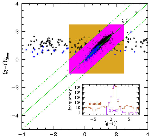
Figure 1: Model versus fibre galaxy colours (both corrected for Galactic extinction) for the sample built with criteria 1-9. Our final selection is highlighted by the magenta region, where only one random galaxy among 4 is plotted for clarity. The asterisks show the galaxies whose model colours are bluer than –1 or redder than 2.5. The crosses show the galaxies whose fibre or model colours fail to meet equation (1). The plus signs display the galaxies whose model and fibre colours are within the limits of equation (1), but whose difference between model and fibre colour is greater than 1 magnitude in absolute value. The blue points represent VYGs according to the STARLIGHT V15 model (see Table 1). The inset shows the distribution of model (brown) and fibre (purple) colours.

We excluded objects with unreliable photometry, analysing their colours (criteria 10 and 11) as follows. Fig. 1 displays the model $(g\!-\!i)^{0}$ colours (corrected for Galactic extinction) as a function of the corresponding fibre colours, as well as the distributions of model and fibre colours. Both the model (brown) and fibre (purple) colours are roughly Gaussian-distributed for

$$-1<(g-i)^{0}<2.5\ ,$$ (1)

but the fibre colours display much fewer outliers. We visually inspected all galaxies whose colours that do not satisfy equation (1) and found that nearly all were contaminated by neighbouring saturated stars or large galaxies. We thus removed from our sample those galaxies whose model or fibre colours do not obey equation (1). The square shaded box in Fig. 1 indicates our colour-filtered sample. We then visually inspected all galaxies whose model and fibre colours both satisfied equation (1), but differed by over 1 magnitude in absolute value. Most of these galaxies were again contaminated by nearby saturated stars or large galaxies. We thus made a second colour selection, requesting that the absolute difference of model and fibre colours be less than unity (magenta region in Fig. 1). This led us to discard an additional 336 galaxies, leaving us with a photometrically accurate sample of 405 022 galaxies. We finally excluded 95 galaxies with negative $\chi^{2}$ values in the spectral fits in any of the 6 spectral models (criterion 12), leaving us with our clean sample of 404 931 galaxies.

2.3 Handling of selection effects

Several observational selection effects can influence our analysis of VYG fractions.

2.3.1 Mass-to-light ratio selection effects

When estimating fractions of VYGs, we must also worry that, at a given stellar mass, galaxies with young stellar populations, which have low mass-to-light ratios, will be more luminous. We must thus ensure that the galaxies with old stellar populations are not missed, hence the fraction of VYGs not overestimated because of this selection effect against high mass-to-light ratio galaxies. Since we are measuring VYG fractions as a function of galaxy stellar mass, a doubly complete survey in volume and luminosity is not complete for the passive galaxies. A sample complete in stellar mass would be desirable, but many more galaxies are found by requesting that the sample is complete in mass-to-light ratio for given mass bins.

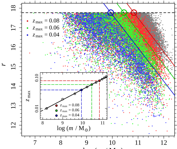
Figure 2: Illustration of the estimation of maximum redshift for completeness at a given stellar mass (for the STARLIGHT / V15 model, see Table 1). Main plot: apparent magnitude vs. stellar mass, for SDSS galaxies in the clean sample, whose $r=17.77$ flux limit is shown as the dashed horizontal line. The full set of galaxies is shown in grey, with galaxies at 3 representative redshifts, $z=0.04$, 0.06, and 0.08, shown in blue, green, and red, respectively, for illustrative purposes, with the corresponding oblique coloured lines representing our estimates of 95th percentiles of mass as a function of apparent magnitude, for that maximum redshift. The large coloured circles indicate the values of $m_{95}(r_{\rm lim})$. Inset: resultant maximum redshift versus stellar mass (with same colour code), with the 3 representative redshifts and corresponding masses shown in colour.

For this, we estimated the maximum redshift for which the subsample of galaxies of a given stellar mass is complete in luminosity (or in mass-to-light-ratio) at our flux limit. This maximum redshift for given mass, $z_{\rm max}(m)$, is estimated in an analogous fashion as Garilli+99, LaBarbera+10, and Trevisan+17. Here, we considered a fine grid of maximum redshifts, $z_{\rm max}$ (in steps of $\Delta z_{\rm max}=0.005$), estimated for each one the 95th percentile in galaxy stellar mass, $m_{95}(r)$, in narrow bins of apparent magnitude $r$, and deduced $m_{95}(r_{\rm lim})$ using a linear fit of $m_{95}(r)$ vs. $r$.

Table 1: Star formation history models

SFH	SSP	acronym	reference	stellar	evol.	IMF	dust	age	metal.	$a_{0}$	$a_{1}$
code	code			library	tracks		model	bins	bins
(1)	(2)	(3)	(4)	(5)	(6)	(7)	(8)	(9)	(10)	(11)	(12)
SL	BC03	S_BC03	Bruzual & Charlot (2003)	STELIB	Padova	Chabrier	screen	15	5	–4.677	0.331
SL	V15	S_V15	Vazdekis et al. (2015)	BaSTI	MILES	Kroupa	screen	15	6	–4.814	0.344
VESPA	BC03	V_BC03_d1	Bruzual & Charlot (2003)	STELIB	Padova	Chabrier	mixed	16	5	–5.218	0.391
VESPA	BC03	V_BC03_d2	Bruzual & Charlot (2003)	STELIB	Padova	Chabrier	2-comp	16	5	–5.228	0.392
VESPA	M05	V_M05_d1	Maraston (2005)	Basel	Padova	Kroupa	mixed	16	4	–5.121	0.382
VESPA	M05	V_M05_d2	Maraston (2005)	Basel	Padova	Kroupa	2-comp	16	4	–5.202	0.390

Notes: The columns are: (1): star formaiton history code (‘SL’ stands for STARLIGHT); (2): single stellar population code; (3): spectral model acronym; (4): reference; (5): stellar library; (6): evolutionary tracks; (7): initial mass function (Chabrier 2003 and Kroupa 2003); (8): dust model (screen, mixed or mixed with additional component around young stars); (9): number of log age bins; (10): number of metallicity bins; (11) and (12): parameters of $z-{\rm max}$ vs. $m$ (eq. [2]).

As seen in the inset of Fig. 2, the relation between maximum redshift and stellar mass is a power law,

$$\log z_{\rm max}=a_{0}+a_{1}\,\log\,\left({m\over{\rm M_{\odot}}}\right)\ ,$$ (2)

whose coefficients are given in Table 1. This constitutes criterion 13. This procedure is illustrated in Fig. 2 for 3 values of $z_{\rm max}$, where the oblique lines indicate the linear fits to $m_{95}(r)$ vs. $r$ and the big circles show the linear extrapolation for $m_{95}(r_{\rm lim})$. The inset of Fig. 2 shows the resulting maximum redshift as a function of stellar mass. There are usually no solutions $z_{\rm max}<0.005$ (below which we do not trust our stellar masses, given the importance of peculiar velocities that reduce the accuracy of redshifts as distance indicators) for $\log\,(m/{\rm M_{\odot}})\leq 8$. The fits of equation (2) and Table 1 are thus only adequate for $\log\,(m/{\rm M_{\odot}})\geq 8$.

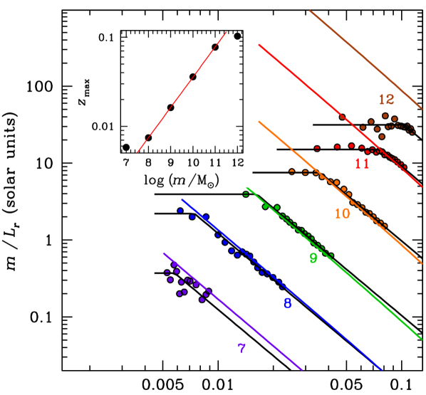
Figure 3: Mass-to-light ratio versus redshift of the clean sample in narrow bins of stellar mass (for the STARLIGHT / Vazdekis et al. 2015 model) of $\log(m/{\rm M_{\odot}})=7$, 8, 9,10, 11, and 12, of respective widths 0.25, 0.15, 0.02, 0.01, 0.01, and 0.02 dex. The symbols indicate the 95th percentiles in equal number bins. The broken black lines show the broken power-law fits for low and high redshift slopes of 0 and –2, respectively, while the straight coloured lines indicate the maximum $m/L_{r}$ given the mass bin maxima and the flux limit. The inset shows the resultant fit of maximum redshift versus mass, with our adopted linear fit (restricted to $8\leq\log\,(m/{\rm M_{\odot}})\leq 11$, red line).

Fig. 3 illustrates this procedure in another fashion. It shows how the variation with redshift of the mass-to-light ratios of galaxies in the clean sample are affected by the flux limit. This is shown for different stellar masses (shown as different colours). The 95th percentiles in equal number bins (circles) show that $m/L_{r}$ is constant with redshift up to some limiting redshift, then decreases as the flux limit leads to a maximum $m/L_{r}$ for given mass and redshift (straight coloured lines), which decreases with increasing redshift. This behaviour is seen for all masses except the lowest mass ($10^{7}\,{\rm M_{\odot}}$), where constant mass-to-light ratio is not seen at low redshifts, nor at the highest mass in $10^{12}\,{\rm M_{\odot}}$, where the flux limit allows for much higher $m/L_{r}$ values than found.

We fitted a broken power-law to each run of $m/L_{r}$ vs. redshift, with slopes of 0 and $-2$. This fit was obtained with a first estimate of the turning point height using the median $\log(m/L_{r})$ of the 25 per cent of the lowest redshifts. Our initial estimate of the turning point redshift used $\hbox{Median}(\log z+0.5\,\log m/L_{r})-\hbox{Median}(\log m/L_{r})$, computed on the 25 per cent highest redshifts. We then minimised $\chi^{2}=\sum\left[\log(m/L_{r})_{\rm data}-\log(m/L_{r})_{\rm model}\right]^{2}$ for the 2 parameters of the broken line break, allowing for $\log m/L_{r}$ and $\log z$ to lie within 0.3 from the first guess. The best-fit broken lines are displayed in black in Fig. 3. The inset to the figure shows the best fit values of $z_{\rm max}$, the abscissa of the breaks of the broken lines in the main figure. One notices that $\log z_{\rm max}$ increases linearly with $\log m$, as $\log z_{\rm max}=-4.849+0.340\,\log(m/{\rm M_{\odot}})$ for the S_V15 model.

Given the similarity between the fits obtained with these two methods, we adopted the relation of equation (2) with the coefficients shown in Table 1, which we assume extrapolate to $m<10^{8}\,{\rm M_{\odot}}$.

2.3.2 Discarding AGN

Although this is not a selection effect, we allow ourselves to discard AGN from our candidate VYGs (criterion 14). For this, we discard VYG candidates that lie above the Kauffmann+03 curve of the BPT diagram.

2.3.3 Aperture effects

The finite (3 arcsec) aperture of the SDSS fibres limits the spectra to the inner regions of many galaxies. Fig. 1 shows that the galaxies that are considered VYGs by one of the spectral models (STARLIGHT V15, see Sect. 3) before filtering by colour and the $\chi^{2}$ of the spectral fits) are associated with blue fibre colours. But there is very little relation between global (model) colour and galaxy youth (blue symbols) estimated from the spectrum measured within the fibre. Many (21 per cent of) galaxies in the clean sample have bluer nuclei than their global bodies (lying below the solid green curve of Fig. 1), leading to spectral fits pointing to a younger stellar population than averaged over the galaxy. For example, the galaxy NGC 838 in the HCG 16 compact group, whose stellar mass is $\approx 5\times 10^{10}\rm\,M_{\odot}$ (O'Sullivan+14a and references therein), has a nucleus (the SDSS fibre subtends an angular radius of 400 pc) whose stellar population has an important very young component (younger than 300 Myr), which accounts for nearly half of the stellar mass of the nucleus, depending on the SFH and SSP model (O'Sullivan+14a), while the bulk of the galaxy is older (Vogt+13). Some of these galaxies with blue nuclei may thus be classified as VYGs even if the bulk of their stellar mass is old.

This aperture effect is potentially serious, since the median fraction of galaxy light subtended by the fibre is only 26 per cent, and only 3 per cent of our sample have fibres covering more than half of the galaxy light. Moreover, building a galaxy sample where the fibres see over, say, 30 per cent of the galaxy light (39 per cent of the sample), leads to an effective cut at higher surface brightness than our limit of $\mu_{r,50}=23$, leading us to lose 99.8 per cent of all galaxies with $21.5<\mu_{r,50}<23$.

Instead, we handle the aperture selection effect by restricting our VYGs to galaxies with blue colour gradients, ${\rm d}(g-i)^{0}/{\rm d}R<0$ (where $R$ is the projected distance to the center), i.e. with a global (model) colour that is bluer than the fibre colour. This constitutes criterion 15.

2.4 Final samples

Table 2: Galaxy samples

Sample	Ages	Size
	(Gyr)	S_V15	V_BC03_d2	V_M05_d2	Gallazzi
clean	all	404 931	404 931	404 931	98 624
liberal VYG	$<\,1$	29 775	5974	5780	303
conserv. VYG	$<\,1$	16 212	3041	3011	124
complete	all	264 847	287 748	291 317	74 836
liberal VYG	$<\,1$	1461	1196	1187	39
conserv. VYG	$<\,1$	649	729	746	15

Notes: The clean galaxy sample is filtered against bad measurements, while the complete one is also complete in mass-to-light ratio. The conservative VYG sample is like the liberal one, except it excludes AGN and galaxies with red colour gradients. Only the main spectral models are shown.

The sample extracted with criteria 1-12 is our clean sample (404 931 galaxies). The sample with criteria 1-13 is our complete sample (typically 280 000 galaxies, depending on the spectral model). We consider two samples of VYGs: liberal samples (one for each spectral model) and a conservative sample that excludes AGN (criterion 14) as well as galaxies with red colour gradients (criterion 15). The two parent samples and the two VYG samples are shown in Table 2.

3 Ages from galaxy spectra

Galaxy SFHs and ages were inferred from the SDSS-DR12 spectra through stellar population synthesis analysis. These spectra have the advantage of fairly high spectral resolution ($R\approx 2000$), excellent signal to noise (above $\sim$20), wide spectral range (from below $3800\,$Å to $9200\,$Å) and they are flux calibrated. They allow to estimate the SFH of each galaxy, by fitting the observed spectrum with the predicted spectrum obtained by the combination of single stellar population (SSP) spectra convolved by the SFH.

We considered three algorithms to estimate the SFH. We used two non-parametric codes: STARLIGHT (CidFernandes+05), which we ran ourselves, and the VESPA database (Tojeiro+09). Both codes fit non-parametric SFHs and metal histories with an internal extinction, considering typically 16 (roughly equally spaced) bins of log age, as well as 4 to 6 bins of metallicity, and a single extinction (see Table 1). This leads to a total of typically $16\times 5+1=81$ free parameters.

We also used the method of Gallazzi+05, who analysed the SFHs of the 175 128 galaxies in the 2nd data release (DR2) of the SDSS. Gallazzi+05 adopted a Bayesian approach to derive median likelihood estimates of stellar population properties such as $r$-band weighted and mass-weighted mean stellar age, stellar metallicity and stellar mass. For each galaxy, observed absorption features were compared with the predictions from a large library of metallicities and SFHs, described by an exponential declining law on top of which random bursts are added, convolved with BC03 SSP models. The probability distribution functions (from which the 16, 50, 84 percentiles are measured) of the light- and mass-weighted mean ages are obtained by marginalising over all the other parameters of the models. We limited our analysis of the Gallazzi+05 sample to the intersection with our clean and complete galaxy samples discarding the 18 per cent of galaxies with no age measurements, with numbers given in Table 1.

All four algorithms have been run using the Bruzual&Charlot03 (Bruzual&Charlot03, hereafter BC03) model to produce synthetic spectra of SSPs to fit the observed SDSS spectra. The SSPs were calculated with the Padova 1994 stellar evolution tracks (Bressan+93; Fagotto+94a; Fagotto+94b; Girardi+96) and with the Chabrier03 initial mass function (IMF). The BC03 model employs the STELIB stellar library (LeBorgne+03). VESPA has also been run using the SSPs of Maraston05 using the Basel stellar library (Lejeune+98) and the Kroupa01 IMF. We also ran STARLIGHT on 424 506 SDSS spectra. STARLIGHT uses the Medium resolution Isaac Newton Telescope Library of Empirical Spectra (MILES, Sanchez-Blazquez+06), using the updated version 10.0 (Vazdekis+15, hereafter V15) of the code presented in Vazdekis+10. These MILES models were computed with the Kroupa01 IMF, and stellar evolution tracks from BaSTI (Bag of Stellar Tracks and Isochrones, Pietrinferni+04; Pietrinferni+06). While STARLIGHT was run assuming a screen dust model, VESPA assumed either a mixed slab interstellar dust model (Charlot&Fall00) or combined it with extra dust around young stars (also from Charlot&Fall00). Gallazzi+05 used a screen dust, with the $\lambda^{-0.7}$ extinction curve used later by VESPA.

The advantage of the STARLIGHT model with the V15 SSP is its recent stellar library and evolutionary tracks, while the VESPA models involve a more refined treatment of dust extinction. The age and metallicity bins of the two SFH codes are quite similar: The lowest age bins are 25 Myr for STARLIGHT and less than 20 Myr for VESPA, while the metallicity bins ranged from $Z=0.0004$ to 0.05 (VESPA BC03) or 0.04 (VESPA M05) or from $Z=0.001$ to 0.048 (STARLIGHT). Note that the lower limit of metallicity of $Z-0.001$ corresponds to the limit of “safe” spectral modeling with the MILES based models (see http://research.iac.es/proyecto/miles/pages/ssp-models/safe-ranges.php).

For each galaxy and for each spectral (SFH and SSP) model (see Table 1), we compute the median age, $\rm age_{50}$, when the stellar mass was half its final value, by linear interpolation of the fractional mass as a function of log age, or use the arithmetic mean mass-weighted age for the Gallazzi model. VYGs are defined as galaxies whose median (or mean for Gallazzi) ages are less than 1 Gyr.

3.1 Tests of the spectral models

We tested the VESPA and STARLIGHT spectral models in several ways.

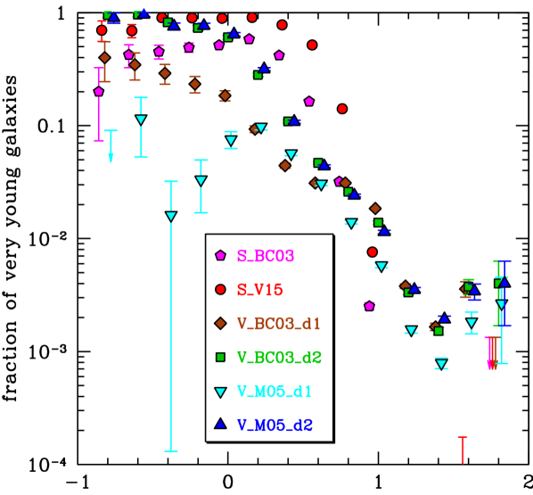
Figure 4: Fraction of very young galaxies (more than half the stellar mass formed in the last Gyr) versus fibre colour, for the STARLIGHT and VESPA spectral models (using the acronyms given in Table 1), for our clean galaxy sample. The error bars are binomial with Wilson 84 percent confidence ($\sim 1\,\sigma$) upper limits. The abscissa are slightly shifted for clarity.

We first check that the fraction of VYGs is very high for the bluest fibre colours. Fig. 4 compares the variation of the VYG fraction with fibre colour for the 6 spectral models. One sees that the VESPA M05 model with 1-component dust fails to achieve a high fraction of VYGs for the bluest colours. Only the STARLIGHT V15 model and the VESPA models with 2-component dust reach high fractions of VYGs at the bluest fibre colours, i.e. over 82 per cent of galaxies with $(g-i)_{\rm fibre}^{0}<-0.1$ are VYGs according to these 3 models, while less than 45 per cent of them are VYGs according to each of the other 3 models.

We then checked that galaxies with the largest H$\alpha$ equivalent widths (EWs) have the greatest fractions of VYGs, close to unity. Indeed, EW measures the ratio of line flux over continuum intensity, which is proportional to the ratio of ongoing or very recent star formation (SF) rate over luminosity, and hence roughly proportional to the ratio of recently formed stellar mass over total stellar mass. Therefore, strong EWs are a sign of high fractions of recently formed stars. This interpretation of the EW is oversimplified, as it depends on the evolution of the stellar mass-to-light ratio, i.e. on the SFH, as well as on the geometrical effects of dust opacity. Nevertheless, according to the STARBURST99 model (Leitherer+99), assuming a Salpeter55 IMF extending to star masses of $100\,\rm M_{\odot}$ and metallicities of $Z_{\odot}/20$, $\rm EW(H\alpha)>500\,$Å indicates ages lower than 50 Myr for a continuous SFH (fig. 84 of Leitherer+99), and lower than only 5 Myr for an instantaneous starburst (fig. 83 of Leitherer+99). These maximum ages are reduced by about a quarter when moving to solar metallicity. For continuous SFH, a burst that started 1 Gyr ago would lead to $\rm EW(H\alpha)=150\,$Å. Of course, if there is an underlying old stellar population at the time of the burst, the continuum would be higher, and the EW reduced. On the other hand, the SFHs computed by VESPA and STARLIGHT do not consider the emission lines, hence they provide an independent estimate of galaxy youth.

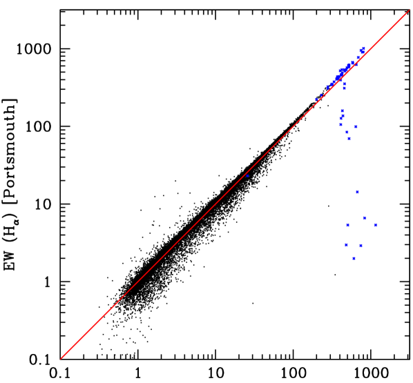
Figure 5: Comparison of the $\rm H\alpha$ equivalent widths between the Portsmouth emission line code (absorption line galaxies have EW = 0) and the MPA/JHU code, which uses the opposite nomenclature (negative EW for emission). Each point is a galaxy (one point in 10 is plotted for clarity) from the clean sample, only keeping galaxies whose EW uncertainties are less than one-third of the absolute value of the EW. 9 galaxies with emission lines according to Portsmouth have absorption lines according to MPA/JHU (thus not shown). The red line denotes equality, while the blue points show all galaxies with very blue fibre colours $(g-i)^{0}<-0.3$.

We first compared two measures of SDSS H$\alpha$ line EWs. The first was taken from the GalSpecLine table (MPA/JHU, Brinchmann+04; Tremonti+04), where the continuum is fitted with linear combinations of BC03-MILES simple stellar population models, similarly to STARLIGHT, and the emission lines are then distinguished from the stellar continuum. The second meaure of EW was extracted from the emissionLinesPort table (Portsmouth, Thomas+13), which is similar to MPA/JHU, but uses the single stellar population model of Maraston&Stromback11, the Gas and Absorption Line Fitting code, GANDALF (Sarzi+06), and Penalized PiXel Fitting, pPFX (Cappellari&Emsellem04). The Portsmouth EW model, which assigns EW = 0 to absorption line galaxies, fails to assign values for 473 galaxies of our clean sample, and assigns astronomically high values of EW (from over $10^{4}\,$Å to over $10^{30}\,$Å) for another 120 galaxies.

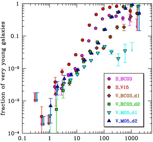
Figure 6: Fraction of very young galaxies (more than half the stellar mass formed in the last Gyr) as a function of the H$\alpha$ equivalent width (determined from the MPA/JHU code) for the STARLIGHT and VESPA spectral models (using the acronyms given in Table 1). We filtered our clean galaxy sample against AGN and for the errors in equivalent width to be lower than 1/3 of the absolute value of the equivalent width. The error bars are binomial with Wilson 84 percent confidence ($\sim 1\,\sigma$) upper limits. The abscissa are slightly shifted for clarity.

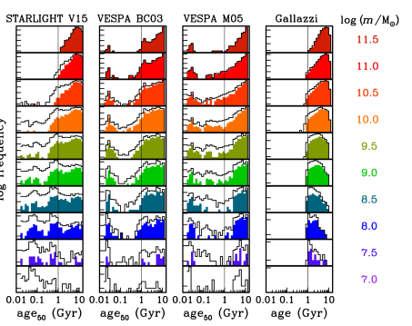
Figure 7: Distribution of the median (mass-weighted mean for Gallazzi) ages of galaxies in the clean SDSS Main Galaxy Sample in bins of stellar mass, for our four spectral models. The open and filled histograms respectively indicate the clean and complete (i.e. limited to $z<z_{\rm max}(m)$, using the fit given in eq. [2] and Table 1) samples. Note that there are no galaxies in the complete sample in the lowest mass bin of all 4 spectral models. The intervals between ticks of log frequency are unity (1 dex).

Fig. 5 compares the EWs between the MPA/JHU and Portsmouth for the 304 418 galaxies for which $0.01\,$Å $<\rm EW(H\alpha)[Portsmouth]<5000\,$Å and for which the absolute value of the EW is at least 3 times its uncertainty for both models. Note that the MPA values use a nomenclature opposite to that of the Portsmouth values: the MPA EWs are negative for emission lines and positive for absorption lines. There is good general agreement between the two measures of H$\alpha$ EW. In particular, all galaxies with $\rm EW(H\alpha)[Portsmouth]>100\,$Å have $\rm-EW(H\alpha)[MPA/JHU]>44\,$Å. However, the converse is not true: among galaxies with $-\rm EW(H\alpha)[MPA/JHU]>100\,$Å, 12 have $\rm EW(H\alpha)[Portsmouth]<44\,$Å, yet most of them have very blue fibre colours, i.e. $(g-i)_{\rm fibre}^{0}<-0.3$ (thick blue points), suggesting very recent SF (at least in the nucleus). While most such galaxies with very blue fibre colours lie on the ridge of equality (taking into account the different sign conventions) between the two measures, and all of them but one have $\rm-EW(H\alpha)[MPA/JHU]>200\,$Å, several galaxies with blue fibre colours have $\rm EW(H\alpha)[Portsmouth]<200\,$Å, and 7 have $\rm EW(H\alpha)[Portsmouth]$ lower than $20\,$Å. This led us to adopt the MPA/JHU values for the H$\alpha$ EWs.

Fig. 6 displays the VYG fractions as a function of the H$\alpha$ EWs. It shows that the VYG fractions generally rise with increasing H$\alpha$ EWs. But the M05 model run with VESPA using a one-component mixed dust model (cyan) gives only a few per cent of VYGs for $\rm EW(H\alpha)>100\,$Å. The corresponding VESPA BC03 model (brown) reaches higher values, but not as high as the VESPA models with a 2-component dust extinction (green and blue). Finally, the BC03 model ran with STARLIGHT (magenta) gives intermediate VYG fractions of $\sim 35$ per cent at these high EWs. In sum, the figure shows that only 3 spectral models stand out in this regard: STARLIGHT with V15 (red), and VESPA with 2-component dust (both BC03 [green] and M05 [blue]), as all three predict that over half the galaxies with $\rm EW(H\alpha)>500\,$Å are VYGs.

The models with the best behaving VYG fractions as a function of fibre colour and H$\alpha$ EW thus appear to be V15 with STARLIGHT, and the 2-component dust BC03 and M05 models with VESPA. We therefore adopt these 3 spectral models in our subsequent analysis of VYGs, and will no longer discuss the other 3 models. We now refer to our adopted spectral models as V15 STARLIGHT, VESPA BC03 and VESPA M05, respectively.

3.2 Comparison between different spectral models

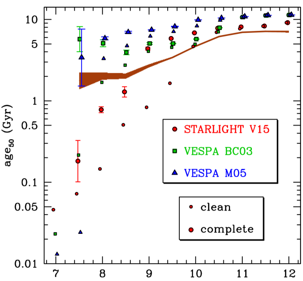
Figure 8: Median (over galaxies within a given mass bin) of ‘median’ stellar ages versus stellar mass for galaxies in the clean (small symbols) and complete (large symbols) SDSS Main Galaxy Sample according to STARLIGHT with the Vaz15 model (red circles), VESPA with BC03 (green squares) and VESPA with Maraston et al. (2005, blue triangles). The brown shaded region shows the mass-weighted arithmetic mean ages from the intersection of the Gallazzi et al. (2005) sample with the complete sample. The error bars (only shown for the complete sample) and the widths of the shaded regions are the uncertainties on the medians from 100 bootstraps.

Fig. 7 shows the distribution of median ages of galaxies according to our 3 adopted spectral models. It confirms the well-known downsizing trend of typically lower masses of galaxies with younger stellar populations. Moreover, the figure shows that the lower age bins are over-represented in the clean sample (open histograms) compared to the complete sample built with $z_{\rm max}(m)$ as described in Sect. 2.3.1 (filled histograms). This effect is especially evident at low mass, where the maximum redshift for completeness is considerably lower (eq. [2], Table 1, Figs. 2 and 3).

Comparing the first three panels of Fig. 7, it seems odd that the two VESPA SFH models, despite their more realistic treatment of dust (a mixed slab instead of a simple screen), assign extremely young ages (less than 80 Myr) to many galaxies at all masses, yet yield only few galaxies with slightly older ages (between 80 and 250 Myr), especially with the BC03 SSP. It is difficult to imagine a universe where the log age distribution of galaxies is so bimodal at all masses. This odd behaviour is not seen in the STARLIGHT V15 model, which shows, within the statistical uncertainties, more continuous distributions of log age for all galaxy masses. The Gallazzi model does not show the extension to very low ages seen in the other models, but this is based on the (arithmetic) mass-weighted mean ages, which are higher than the median ages.

Fig. 8 summarises the differences between the SFH/SSP models by showing the median (over mass bins) of the median age versus galaxy stellar mass. One notices important differences between the models at low galaxy stellar mass. In the clean sample (small points), the 2 VESPA models show a jump in age₅₀ at low masses, while the increase is more gradual with STARLIGHT V15. On the other hand, the complete sample shows high ages at low mass with the VESPA models compared to low ages at low mass for the STARLIGHT model. In other words, STARLIGHT V15 predicts a strong downsizing down to low masses, while the downsizing trend is weaker for the VESPA models, with signs of reaching a plateau at low mass (and perhaps even upsizing with VESPA BC03). In any event, the median ages of galaxies are enhanced when switching from the clean sample to the complete sample, especially for the STARLIGHT V15 model, but least so for VESPA M05.

Fig. 8 also displays the mass-weighted arithmetic mean ages for the intersection of our complete sample (with S V15) with the sample extracted from Gallazzi+05, shown as the brown shaded region.

4 Results

4.1 Fraction of very young SDSS galaxies versus mass

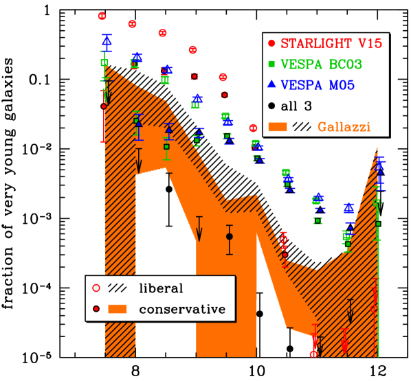
Figure 9: Fraction of very young galaxies (half the stellar mass formed less than 1 Gyr before the epoch corresponding to the galaxy’s redshift) versus stellar mass for the complete SDSS sample. The open symbols and dashed shaded region indicate the fractions of liberal VYGs for the 3 SFH models and the Gallazzi model, respectively, while the solid symbols and orange shaded region show the corresponding fractions of galaxies in the complete sample that are conservative VYGs (not AGN and with bluer global (model) colours than the fibre colours). The true fraction of VYGs should lie in between the two sets of symbols. The black filled circles are the fractions of the galaxies that are liberal VYGs for all 3 models (the log masses are the means of the 3 spectral models with weights 1/2 for STARLIGHT and 1/4 for the two VEPSA models). The errors are binomial with Wilson 90 per cent confidence upper limits. The abscissas are slightly shifted for clarity.

We now arrive at the focus of our analysis: the fraction of VYGs as a function of galaxy stellar mass. Fig. 9 shows the fraction of VYGs versus galaxy mass for the complete sample of SDSS galaxies, using the 3 spectral models, as well as that of Gallazzi+05. These models are shown for both the liberal and conservative (‘not AGN & $\nabla(g-i)^{0}<0$’) VYG samples.

For all 3 spectral models, the liberal VYG fractions (open symbols in Fig. 9) decrease with increasing mass. The STARLIGHT V15 model gives VYG fractions $>$3 per cent at low masses ($m$ $<$ $10^{10}\,{\rm M_{\odot}}$) and 50 per cent at the lowest securely complete mass, $m$ = $10^{8.5}\,{\rm M_{\odot}}$ (see Sect. 2.3.1). In comparison, the two VESPA models lead to VYG fractions over 1 per cent at low masses ($m$ $<$ $10^{10}\,{\rm M_{\odot}}$) and to 12 per cent at $m$=$10^{8.5}\,{\rm M_{\odot}}$. However at high masses, the VESPA models produce a slowly decreasing VYG fraction with increasing mass, while the STARLIGHT V15 model gives a sharply decreasing VYG fraction for $m$ $>$ $10^{10}\,{\rm M_{\odot}}$, 1–2 orders of magnitude lower than the VYG fractions found in VESPA models.

As discussed in Sect. 2.3.3, a serious concern is that the SDSS 3 arcsec diameter fibre is often limited to the light from the central regions of extended galaxies. We may thus mistakenly identify a galaxy as very young, while it may be an old galaxy with a very young nucleus. Hence, in Fig. 9, we also plot the fraction of galaxies in the complete sample that are conservative VYGs, i.e. that are not AGNs, and with global colours that are bluer than their fibre colours. The liberal VYG sample may be contaminated by AGN and by galaxies that are young according to their fibre colours but older globally. On the other hand, the conservative VYG sample may miss galaxies that are extremely young in the region covered by the SDSS fibre but that are still very young (but redder and older) overall. The true fraction of VYGs should thus lie somewhere between the liberal and conservative VYG fractions, i.e. they are delimited by the open and filled symbols in Fig. 9.

While the conservative estimates of the VYG fractions resemble the liberal estimates at high mass, they yield flat trends of VYG fractions at $m<10^{10}\,{\rm M_{\odot}}$ for the VESPA spectral models. Hence, for the 3 adopted spectral models, the difference between the lower and upper limits of the VYG fractions is only important at low mass.

The black points in Fig. 9 represent our most conservative estimate of the VYG fraction. We obtained these ‘3-way VYG’ fractions by requesting that all 3 spectral models agree that the median age of conservative VYG candidates is less than 1 Gyr, leading to only 9 3-way VYGs over all masses. The shaded regions in Fig. 9 show that the fractions of VYGs derived from the Gallazzi model (using mass-weighted ages) are typically 10 times lower than with the STARLIGHT and VESPA models.

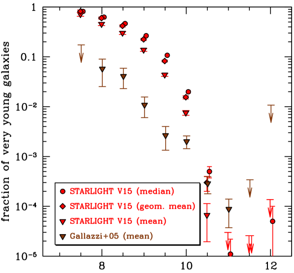
Figure 10: Effect of the definition of age in the fraction of liberal very young galaxies in the complete sample as a function of stellar mass. The galaxy ages are computed as medians (circles), or mass-weighted with geometric means (diamonds) or arithmetic means (triangles), for STARLIGHT V15 (red) and the Gallazzi model (brown). The error bars are binomial with 90 per cent Wilson upper limits. The abscissa are slighted shifted for clarity.

Since the SFHs of VYGs are not Gaussian in time but have long high-age tails, the arithmetic mean mass-weighted age will be greater than the corresponding median age. This implies that the VYG fractions defined with arithmetic mean mass-weighted ages should be smaller than with median ages. Fig. 10 confirms this idea using the STARLIGHT V15 model: the VYG fractions are indeed lower with arithmetic mean mass-weighted ages instead of median ages, in particular at intermediate and high masses for the complete sample, where the decrease reaches a factor 4 (while the VYG fractions obtained with the mass-weighted geometric mean ages are only slightly lower than those found with the median ages). Nevertheless, the Gallazzi model (using mean ages) yields even lower VYG fractions than the STARLIGHT V15 model using similarly defined mean mass-weighted ages.

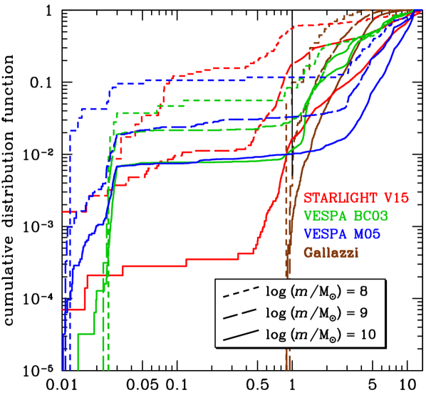
Figure 11: Cumulative distribution functions of median (mass-weighted mean for Gallazzi) age for galaxies in the complete sample, for the four spectral models and for 3 mass bins of width $\pm 0.5$ dex. The vertical line illustrates our choice of 1 Gyr for defining VYGs.

One question of interest is how the VYG fractions vary when the maximum median age is changed to values below or above 1 Gyr. Fig. 11 illustrates the distribution of median ages for the 3 spectral models and in 3 bins of stellar mass. This allows us to estimate the fraction of galaxies younger than any chosen age. For example, with STARLIGHT V15, the fraction of galaxies younger than 100 Myr is typically one order of magnitude lower than the fraction of galaxies younger than 1 Gyr (our VYGs). In contrast, the VESPA models indicate nearly identical fractions of galaxies younger than 100 Myr and younger than 1 Gyr. This difference is related to the wide gap between 30 Myr and 500 Myr in the distribution of ages seen in Fig. 7 for these models (see the filled histograms corresponding to the complete sample). Finally, whereas the Gallazzi model produces only rare galaxies younger than 1 Gyr, it produces roughly the same fraction of galaxies less than 2 Gyr than the other 2 SFH codes.

5 Discussion

5.1 Summary of results

The spectral analyses of SDSS galaxies with different SFH codes and different single stellar population models lead to different age-mass relations (Fig. 8). STARLIGHT shows downsizing at all masses down to the limit of $\log\,(m/{\rm M}_{\odot})=8.5$ where we are confident that the data is complete, while VESPA gives a rough plateau in age at masses below $10^{10}\,{\rm M_{\odot}}$ and Gallazzi is in between.

The derived VYG fractions fall with increasing mass, with possibly as many as 50 per cent (STARLIGHT V15, liberal) at $\log\,(m/{\rm M}_{\odot})=8.5$ to less than half a per cent at $\log\,(m/{\rm M}_{\odot})=10.5$. The VESPA models show a shallower slope ($\approx\!\!-1.5$) with stellar mass than STARLIGHT ($\approx\!-3$). Thus, VESPA models predict that VYGs should occur at high masses, while STARLIGHT V15 does not. The spectral model of Gallazzi+05 yields VYG fractions that resemble the lower VESPA fractions at low mass and the lower STARLIGHT fractions at high mass.

5.2 Caveats

Estimating the fraction of VYGs from SDSS spectra is difficult for several reasons.

1. The SDSS spectra are limited to the inner regions of the galaxies, hence do not provide a global view of the SFH of each galaxy. We considered this aperture effect in our conservative VYG sample, which discards not only AGN, but also VYG candidates with red colour gradients. The true VYG fractions ought to lie in between our liberal and conservative estimates.

2. Individual SFHs of galaxies suffer from degeneracies caused by their different epochs of SF, their metallicities, and their galactic extinction in the inner region sampled by the SDSS fibre. In fact, old stellar populations may not be revealed by the SFH modelling, as we will discuss in Sect. 5.8.

3. Our SFHs neglect stellar evolution and the disappearance of high-mass stars exploding as type II supernovae. Indeed, the VESPA code does not consider these effects, and for consistency we have chosen to use the same approach with STARLIGHT.

   

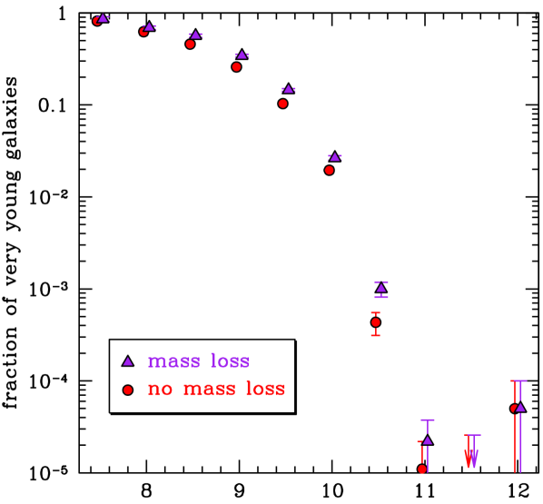
   Figure 12: Effect of considering mass loss in the fraction of VYGs versus stellar mass, using the STARLIGHT V15 model on the complete sample. The error bars are binomial, with 90 per cent Wilson upper limits. The abscissa are shifted for clarity.

   Supernova explosions affect massive stars that are short-lived, thus depleting more the stars formed earlier. Similarly, mass loss from stellar evolution takes time, thus decreases more the stars formed earlier. So both type II supernovae and stellar evolution should result in enhanced VYG fractions. Fig. 12 confirms that mass loss does raise the VYG fractions, but never more than by 0.2 dex for low and intermediate galaxy stellar masses ($\log\,(m/{\rm M}_{\odot})\leq 10$).

4. There is disagreement between different spectral models using the same SFH code (e.g. BC03 vs. M05 with VESPA) and using different SFH codes (e.g. STARLIGHT vs. VESPA).

5. The spectral models may lead to worse fits for low-mass galaxies, which show the highest fractions of VYGs.

   

   

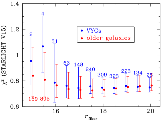
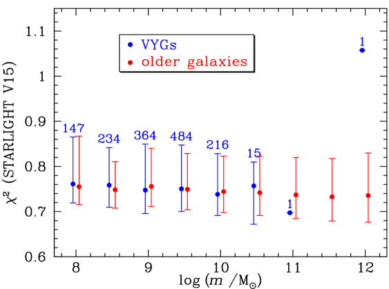
   Figure 13: Spectral fit quality (reduced $\chi^{2}$) for the STARLIGHT V15 fits on the complete sample, as a function of the fiber magnitude (proxy for the signal to noise of the spectrum, top) and of the galaxy stellar mass (bottom), for both the VYGs (blue and the older galaxies (red). The symbols denote medians, while the error bars represent 16th and 84th percentiles. The numbers above the error bars indicate the number of VYGs per bin.

   The top panel of Fig. 13 shows how the reduced $\chi^{2}$ of the spectral fit varies with fiber magnitude. Since all observations are in the same angular aperture of 3 arcsec, fiber magnitude is directly linked to the mean surface brightness in the fibre, which is an excellent proxy for the signal to noise ratio of the continuum. The figure indicates that for $r_{\rm fiber}>15.75$, the spectral fits of the VYGs are only slightly worse than those of the older galaxies. This is likely due to the enhanced emission lines in the spectra of VYGs (see Sect. 5.6 and Fig. 19 below). However, at very bright fiber magnitudes, the spectral fits are marginally worse for the VYGs (as the numbers on the figure attest, this only concerns 6 galaxies, of which 4 have $\chi^{2}>1$). However, the older very bright galaxies also show a stronger dispersion in $\chi^{2}$ than less bright galaxies of the same age range, and their high numbers attest that this higher dispersion is statistically significant. The bottom panel of Fig. 13 shows that the spectral fits of VYGs and older galaxies differ very little when $\chi^{2}$ is plotted versus galaxy stellar mass.

   We also ran STARLIGHT V15 for I Zw 18, whose stellar mass is only $10^{7}\,{\rm M}_{\odot}$ (Papaderos&Ostlin12; Izotov+18). We found a median age of only 30 Myr (our lower allowed age), with 100 per cent of the stars younger than 100 Myr. Theses ages are much lower than those derived from CMDs (less than 500 Myr according to Izotov&Thuan04 and over 1 Gyr according to Aloisi+07). This galaxy is known to have strong nebular emission, not only in lines (EW(H$\alpha)=410\,\rm\AA$), but also in the continuum (Papaderos&Ostlin12). However, in the spectral range of SDSS, the contribution of the nebular emission to the continuum rises with wavelength, reaching half of the continuum at 8200$\,\rm\AA$ (fig. 9b of Izotov+11). Since we do not subtract the nebular contribution to the continuum, the galaxy appears redder, leading the spectral modeling of stellar populations to overestimate the ages. Therefore, according to STARLIGHT V15, the median age of I Zw 18 should be even lower than 30 Myr.

6. Regardless of the quality of the fits, it is very difficult to extract SFHs of galaxies with non-negligible young stellar populations, since young stars have so high luminosity/mass ratios compared to older ones.

5.3 Comparison to the literature

The only other study known to us in estimating fractions of very young galaxies per bin of stellar mass is that of Dressler+18. These authors derived SFHs from galaxy SEDs defined by $R=20-50$ prism observations in the optical band, combined with $ugrizJK$ broadband photometry, following the prescriptions described in Dressler+16. They used single stellar population models from Conroy+09, based on the BaSeL 3.1 library (Lejeune+98), the Padova isochrones (Marigo&Girardi07; Marigo+08), and an IMF that is virtually identical to that of Chabrier03.

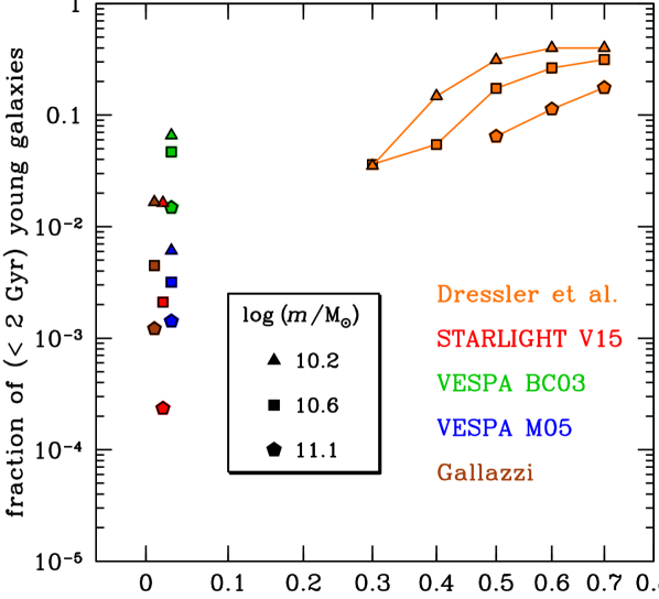
Figure 14: Comparison of our analysis of the SDSS Main Galaxy Sample with the analysis of Dressler et al. (2018) of a higher redshift sample of the mass dependence of the fraction of ‘young’ galaxies, defined here to have over half their stellar mass formed within 2 Gyr before the epoch of observation, versus redshift in 3 bins of stellar mass. The SDSS fractions (i.e. low redshift) are for the conservative definition using the complete sample, with slightly shifted abscissas for clarity.

Note that Dressler+18 selected their galaxies at $3.6\,\rm\mu m$, i.e at typically $2.2\,\rm\mu m$ in the rest frame. While galaxies evolve more slowly in the near-IR than in the optical $r$ band used in SDSS, there is still significant evolution of the mass-to-light ratio in the $K$ band between 1 and 13 Gyr for single stellar populations, by a similar fraction as in the $r$ band (see. fig. 5 of Charlot&Bruzual91), but there is no evolution of $M/L_{K}$ after 4 Gyr, contrary to $M/L_{r}$. Therefore, the sample of Dressler+18 may be incomplete for high mass-to-light ratio galaxies. However, we noted in Sect. 2.3.1 that this incompleteness is smaller at the high stellar masses probed by Dressler+18.

As seen in Fig. 14, the young galaxy fractions measured by Dressler+18 decrease with decreasing redshift, as expected, since the redshifts considered are past the cosmic noon ($z\approx 2$), the epoch when the cosmic star SF rate density is highest. The comparison of their fractions with ours involves an extrapolation of their fractions to the low redshifts probed by the complete subsamples of the SDSS/MGS ($\left\langle z\right\rangle\approx 0.07$). The high young galaxy fractions found with the VESPA BC03 spectral model (also seen in Fig. 11 for these high masses) appear inconsistent with these extrapolations. However, there is no obvious conflict between the young galaxy fractions found by Dressler+18 and those deduced from our other three spectral models.

5.4 Star formation histories

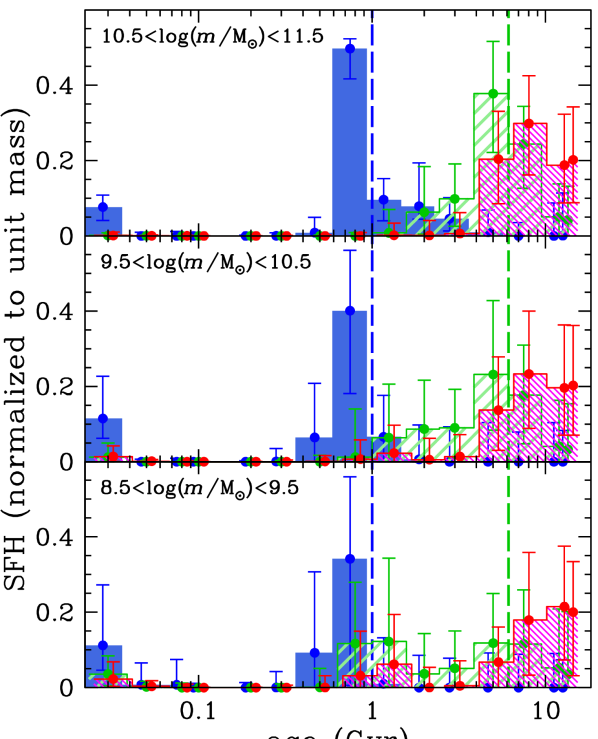
Figure 15: Star formation histories for VYGs (blue), intermediate age galaxies ($1<\rm age_{50}<6.1\,Gyr$, green) and old galaxies ($\rm age_{50}>6.1\,Gyr$, red) for 3 bins of final stellar mass, for the STARLIGHT V15 model, using the complete sample. These star formation histories account for stellar evolution and the disappearance of massive stars by supernova explosions. The points indicate the median star formation history, while the error bars indicate 16th and 84th percentiles. The vertical dashed lines delimit the maximum allowed median ages for the very young and intermediate galaxy classes.

One can go further and ask whether the SFHs of VYGs are such that the distribution of stellar ages has a narrow peak slightly below 1 Gyr or is more spread out. We also explore how these SFHs vary with final galaxy stellar mass, and how varied are the SFHs of VYGs of given stellar mass.

Fig. 15 displays, for 3 bins of $z$=0 stellar mass, the SFHs of VYGs (blue symbols) as well as of intermediate-age galaxies, which we define as having median ages between 1 and 6.1 Gyr, and of old galaxies (older than 6.1 Gyr). The figure shows the STARLIGHT SFHs, accounting for stellar evolution and the disappearance of massive stars from type II supernova explosions.

At high mass, the VYGs display an intermediate-age (1-4 Gyr) stellar population, and virtually no population younger than 600 Myr, except for an extremely young population of 30 Myr. This is probably an unavoidable artefact of the over-sensitivity of SFH codes to very young stellar populations. At lower masses, the VYGs no longer display the 1-4 Gyr population, but progressively enhance their younger 0.4-0.6 Gyr population. In other words, the SFHs of VYGs, expressed in log age, are positively skewed at high masses and negatively skewed at low masses. One also notices an increase in the diversity of the SFHs of VYGs towards lower galaxy stellar masses. Similar trends are seen for intermediate-age galaxies (green symbols), indicating a general trend of higher age diversity at lower masses (see Fig. 7).

5.5 Comparison to predictions from models of galaxy formation

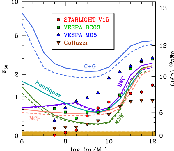
Figure 16: Median (over each mass bin) of median stellar ages versus galaxy stellar mass, measured in the complete sample of the SDSS Main Galaxy Sample with 3 spectral models (symbols) and predicted in galaxy formation models (lines): the physical model of Cattaneo et al. (2011) with a more realistic truncation at low mass from Gnedin (2000) [C+G] (royal blue), the empirical (abundance matching) models of Moster et al. (2013) [MNW] (olive green) and Behroozi et al. (2013) [BWC] (violet), where all three model the stellar mass a a function of halo mass and redshift; the model of Mutch et al. [MCP] (salmon), which has the stellar mass growth rate as the halo mass growth rate times a function of halo mass and redshift, and the Henriques et al. (2015) [Henriques] SAM (blue-green) run on the Millennium II simulation (Boylan-Kolchin et al. 2009) for centrals only. The solid and dashed lines show the analytical galaxy formation models with the bursty and quiet halo merger schemes, respectively. The orange shaded region highlights very young galaxies.

We now compare the spectral models in this paper with the galaxy formation models described in Paper I (Tweed+18). There, we had considered three analytical models where the galaxy stellar mass is a function of $z$=0 halo mass and redshift: one physical model (Cattaneo+11), improved with a more realistic cut off at low halo masses from the hydrodynamical simulations of Gnedin00 [C+G], and two empirical models (Moster+13 [MNW], Behroozi+13 [BWC])] that use abundance matching to link galaxy stellar masses with their halo masses. We also considered a model where the galaxy stellar mass growth rate is equal to its halo mass growth rate times a function of the $z$=0 halo mass and of redshift (Mutch+13 [MCP]). Finally, we considered the SAM of Henriques+15, which has the advantage of having environmental effects implicitly incorporated, but the disadvantage of worse mass resolution and poorer statistics. Note that the galaxy formation models were limited to central galaxies, either explicitly (for Henriques) or by construction of the Monte-Carlo halo merger trees (analytical models), while the spectral models were run on all galaxies. However, in Paper I, we found that the fraction of VYGs differs little between centrals and satellites in the Henriques SAM.

Fig. 16 compares the age-mass relations of the galaxy formation models derived in Paper I with those of the spectral models (also shown in Fig. 8). The spectral models exhibit a shallower decrease of ages with decreasing stellar mass (i.e. shallower downsizing of mass) between $\log\,(m/{\rm M}_{\odot})=10$ to 11.5. While several galaxy formation models (C+G, MNW, and Henriques) predict upsizing at masses below $10^{9}\,{\rm M_{\odot}}$, this is not seen in the spectral models run on SDSS galaxies, except in the VESPA BC03 model.

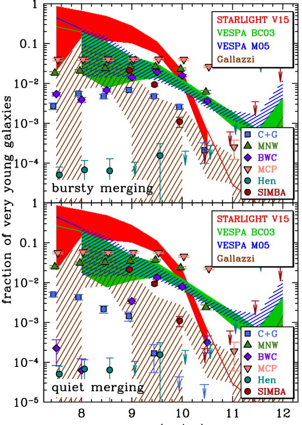
Figure 17: Fraction of very young galaxies versus stellar mass: constraints from the complete sample of SDSS galaxy spectra (shaded regions and lines) confronted to the predictions from the galaxy formation models (symbols, with same acronyms as in Fig. 16) of Paper I, for bursty (top) and quiet (bottom) halo merging. The upper and lower envelopes of the shaded regions are respectively the 84th percentiles of the liberal VYG sample and the 16th percentiles of the conservative VYG sample (no AGN and blue colour gradients). The lines are the 84th percentiles of the liberal VYG sample. The error bars for the ‘Hen’ (Henriques et al. 2015) SAM and the SIMBA simulation (Davé et al. 2019) are binomial and the upper limits are $1\,\sigma$. In the first 4 models, the galaxies are weighted, hence the error bars are estimated from 100 bootstraps.

Can the differences in the VYG fractions of SDSS galaxies obtained with different spectral models and/or different (conservative/liberal) treatments of the selection effects be understood by comparing those results to the predictions of VYG fractions from models of galaxy formation? Fig. 17 compares the VYG fractions derived from the SDSS spectra with the predicted fractions from galaxy formation models obtained in Paper I, the only study known to us that uses galaxy formation/evolution models to predict the fractions of VYGs versus stellar mass. The two panels are for the two schemes of halo merging, one that comes with starbursts, and the other one that does not.

One first notices that the different galaxy formation models display a much wider range of predicted VYG fractions than the spectral models do, although in the bursty halo merging scheme the analytical models agree fairly well with one another. It is the SAM that disagrees the most by predicting orders of magnitude fewer VYGs.

The VYG fractions predicted by the galaxy formation models vary little with galaxy stellar mass, while the spectral models predict decreasing liberal VYG fractions with increasing stellar mass. One exception is the BWC model in the quiet merging scheme, which shows a peak in VYG fraction at $\log\,(m/{\rm M}_{\odot})=9.5$.

The match between the VYG fractions versus mass based on galaxy formation model predictions and on spectral modelling is generally not good. In particular, the STARLIGHT spectral model yields much higher conservative VYG fractions at $m<10^{9}\,{\rm M_{\odot}}$ than any galaxy formation model predicts. Also, the Henriques SAM predicts at least 100 times lower VYG fractions than even the conservative spectral models. At $m=10^{8.5}\,{\rm M_{\odot}}$, the Henriques SAM predicts 1000 times fewer VYGs than the conservative estimate of the STARLIGHT V15 model. However a closer look reveals that, in the bursty halo merging scheme, the BWC model predicts VYG fractions that match well the VESPA VYG fractions.

Fig. 17 also shows the first predictions of the fractions of VYGs versus stellar mass at $z=0$ from a cosmological hydrodynamical simulation, here the $100\,h^{-1}\,\rm Mpc$ SIMBA simulation (Dave+19). This simulation has a more refined treatment of AGN feedback for low and intermediate mass galaxies, and reproduces better observational properties of galaxies at $z=0$ than analogous simulations of the same resolution in space and mass ($1\,h^{-1}\,\rm kpc$). Moreover, hydrodynamical simulations should be more realistic than the analytical models and the SAM, thanks to their much better spatial resolution and their more refined subgrid physics (in particular the AGN feedback in SIMBA). The VYG fractions found in SIMBA are much higher than in the SAM (up to over 300 times at $\log\,(m/{\rm M}_{\odot})=9$), but comparable to the analytical models, and quite similar to the upper envelope of the Gallazzi spectral models. However, the VYG fractions are overestimated at the lowest masses, because galaxies near the lowest resolved mass cannot form early and galaxy formation is delayed, as we found in Paper I for the Henriques SAM run on the lower resolution Millennium simulation. In the SIMBA simulation, the SFHs appear to have converged for 256 star particles, corresponding to $\log\,(m/{\rm M}_{\odot})=9.3$.

5.6 Comparison to emission-line galaxies

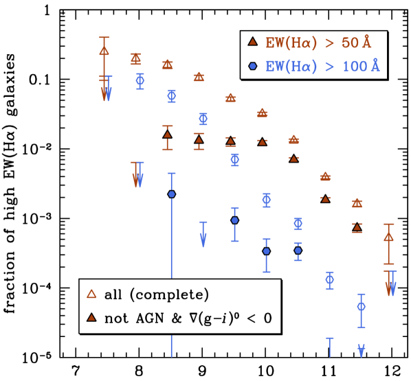
Figure 18: Fraction of galaxies in complete sample (for all 3 spectral models) that have their H$\alpha$ emission-line with equivalent width (determined from MPA/JHU, now using the sign convention of positive EW for emission lines) above a threshold, as a function of the mean of the log masses of the 3 spectral models (with weights 1/2, 1/4, and 1/4 for STARLIGHT V15, VESPA BC03, and VESPA M05, respectively. The open symbols are the fraction of high EWs among all galaxies in the complete sample, while the filled symbols represent the fraction of galaxies in the complete sample that have high EWs, are not AGN and have blue colour gradients. The error bars are binomial with 90 per cent Wilson upper limits. The abscissa are slightly shifted for clarity.

Strong emission lines in galaxy spectra are another indicator of very young stellar populations. As already mentioned in Sect. 3.1, by measuring the ratio of the line flux over the continuum, the EW of an emission line essentially measures the ongoing SF rate over its integral over time, which to first order is the specific SF rate. According to Leitherer+99 using the starburst99 code, a single burst of SF is characterised by an (H$\alpha$) EW that decreases 4 Myr after the burst as $t^{-4}$, becoming negligible ($<0.1\,$Å) after 1 Gyr. On the other hand, if the SF rate is uniform in time, the EW falls off much more slowly, roughly as $t^{-1/3}$, leading to values of 30 and 150 Å, depending on whether the initial mass function is truncated at 30 or $100\,{\rm M_{\odot}}$ at the high end.

Fig. 18 displays the fraction of galaxies with high EWs; 1) those with EW $>$ 50 Å and 2) those with EW $>$ 100 Å. These fractions decrease with increasing mass, roughly in the same way as the fractions of VYGs. In particular, the conservative case of the fraction of galaxies in the complete sample that have high H$\alpha$ EWs $>$ 50 Å, are not AGN, and have blue colour gradients (solid symbols), shows the same plateau at $\simeq 1.5$ per cent as does the fraction of VYGs with the same constraints in the two VESPA models (Fig. 9).

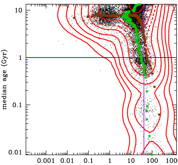
Figure 19: Median age (from the STARLIGHT V15 model fit to the continua of SDSS spectra) versus H$\alpha$ equivalent width (from MPA/JHU) for the non-AGN galaxies in the clean sample. Only 1 random galaxy among 20 is shown, while the contours (in steps of 0.5 dex in density – and 2 intermediate ones shown by dashes – estimated in 40$\times$40 cells) are for the full galaxy sample (the limits of the figure correspond to the limits of the data, after discarding systems with $\rm-EW(H\alpha)<0$). The horizontal blue line corresponds to a median age of 1 Gyr (7th percentile), while the vertical purple line corresponds to $\rm-EW(H\alpha)=41\,\AA$ (93rd percentile). The brown circles show the medians of the median ages in equal number bins of EW (1000/bin), while the green circles show the medians of EW in equal number bins of median age.

Fig. 19 compares the ages and H$\alpha$ EWs of the clean galaxy sample. One notices 3 classes of galaxies in this figure: a class of low EW with high ages (upper left clump of points), a dominant class of moderately high EW with high ages (upper right clump), and a class of somewhat higher EW and low ages (lower clump). Admittedly, the bimodal distribution of galaxy ages (even with STARLIGHT, see Fig. 7) may be an artifact of the spectral modeling of the SFHs. Note that the dominant clump of high-EW old galaxies cannot be AGN, since we had filtered these out of the clean sample for this figure. Fig. 19 displays a clear anti-correlation between ages and EWs ($r=0.37$ from a Spearman rank correlation test, with a null $p$ value). However, one might have hoped for an even stronger correlation, as can be seen by the disagreement in the trajectories of median age vs EW (brown) and its transpose (green).

Telles&Melnick18 analysed a sample of galaxies with EW(H$\alpha)>50$ Å, EW(H$\beta)>30$ Å and a rectangular selection of the upper left portion of the BPT diagram. They fit parametric three-burst SFHs to the spectral energy distributions of these galaxies from the ultraviolet (UV) to the mid-IR. They found that the ‘young’ stellar population contributes to typically less than 2 per cent of the stellar mass of their emission-line galaxies, and never more than 8 per cent. However, their ‘young’ population is defined to be less than 10 Myr old, and unfortunately they do not provide the fraction of stellar mass in galaxies in their ‘intermediate’ age population which spans 100 Myr to 1 Gyr in age.

5.7 Number of very young galaxies in the SDSS Main Galaxy Sample

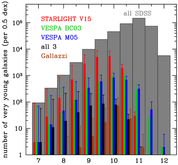
Figure 20: Observed numbers of SDSS Main Galaxy Sample galaxies in clean sample (grey bars) and numbers of conservative (thick bars) and liberal (error bars) very young galaxies in the clean sample, all as a function of stellar mass (averaged over the 3 models as in Fig. 9). The black bars represent the subsample of these very young galaxies that are classified as very young in all three spectral models.

Given the non-negligible fractions of VYGs, how many VYGs may lurk in the SDSS Main Galaxy Sample? Fig. 20 displays the numbers of VYGs in the clean sample for the different spectral models, as well as the numbers of galaxies that are VYGs for all three spectral models (black bars).

The SDSS spectra analysed by STARLIGHT and VESPA lead to thousands of conservative VYGs in the clean samples of the SDSS/MGS (16211, 3040, and 3010 for the STARLIGHT V15, VESPA BC03, and VESPA M05 spectral models, respectively). These spectral estimates lead to peaks in the number of VYG galaxies in the SDSS/MGS around $m=10^{10}\,{\rm M}_{\odot}$. This would mean that VYGs like I Zw 18, but much more massive, are not so rare, but rather ubiquitous.

There is also a large discrepancy in the predicted number of VYGs at large stellar masses, between the VESPA models, according to which there are many VYGs with masses higher than $10^{11.25}\,{\rm M_{\odot}}$ and the STARLIGHT V15 model, whose most massive VYG has $m=10^{10.82}\,{\rm M_{\odot}}$. The most massive conservative VYG found by all three spectral models has $\log\,(m/{\rm M}_{\odot})=10.35$ (STARLIGHT V15), 10.93 (VESPA BC03), 11.05 (VESPA M05), and corresponds to the same galaxy. Its weighted log mass is $\log\,(m/{\rm M}_{\odot})=10.67$.

5.8 Can VYGs contain hidden old stellar populations?

The higher fraction of VYGs found in our analysis of SFHs derived from SDSS spectra, in comparison with the predictions from nearly all galaxy formation models (Fig. 17), suggest that old stellar populations may be present in VYGs, but are hidden from our view and do not contribute strongly to the SED. By selecting conservative VYGs that have bluer global colours than their fibre colours, we have attempted to eliminate galaxies that possess an old extended stellar population underlying the young stellar population. However, the old stellar population may have no effect on the global colour within the extent of the galaxy in the SDSS image, and yet become increasingly important with radius, dominating the integrated stellar mass at large radii.

We examine this situation by considering the following simple model. Assume that the galaxy is composed of two stellar populations, one young and one old, which both follow Sérsic surface brightness profiles,

$$\Sigma(\theta)=\Sigma(0)\,\exp\left[-b(n)\left({\theta\over\theta_{\rm e}}\right)^{1/n}\right]\ ,$$ (3)

where $b(n)\simeq 2\,n-1/3+0.009876/n$ (Prugniel&Simien97), with effective (half-light) radii, $\theta_{\rm young}$ and $\theta_{\rm old}$, indices $n_{\rm young}$ and $n_{\rm old}$, and with very different mass-to-light ratios, $\Upsilon_{\rm young}$ and $\Upsilon_{\rm old}$, both assumed to be independent of radius. Our model includes the additional constraint that each population contributes to half the total stellar mass within the fibre. This is a conservative assumption, since our VYGs are selected to contain at least half their stellar mass younger than 1 Gyr. We also assume that the young population has a Sérsic index $n_{\rm young}=1$ as expected for exponential disks and choose $\theta_{\rm young}=3^{\prime\prime}$ (close to the median of the conservative VYGs of 2.9 arcsec in the clean sample).

Given that the integrated stellar mass (or luminosity), in cylindrical apertures, of the Sérsic model follows (see Graham&Colless97)

$$m(\theta)={2\pi\,n\over b^{2n}(n)}\,\gamma\left[2n,b(n)\left({\theta\over\theta_{\rm e}}\right)^{1/n}\right]\,\Sigma_{0}\,d^{2}\,\theta_{\rm e}^{2}\ ,$$ (4)

where $\Sigma_{0}$ is the central surface mass density, $d$ is the (cosmological angular) distance and $\gamma(a,x)$ is the lower incomplete gamma function, the ratio of total old mass over total young mass is

$${m_{\rm old}\over m_{\rm young}} ={\left[m(\theta_{\rm fib})/m\right]_{\rm young}\over\left[m(\theta_{\rm fib})/m\right]_{\rm old}}$$ (5)

$$={P[2n_{\rm young},b(n_{\rm young})\left(\theta_{\rm fib}/\theta_{\rm young}\right)^{1/n_{\rm young}}]\over P[2n_{\rm old},b(n_{\rm old})\left(\theta_{\rm fib}/\theta_{\rm old}\right)^{1/n_{\rm old}}]}\ ,$$ (6)

where $P(a,x)=\gamma(a,x)/\Gamma(a)$ is the lower regularised gamma function and where equation (5) comes from the equal contributions of the young and old populations to the mass within the fibre.

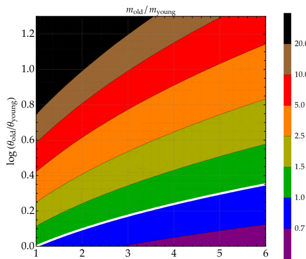
Figure 21: Ratios of old over young total masses, $m_{\rm old}/m_{\rm young}$ (eq. [6]) as a function of the Sérsic index of the old population, $n_{\rm old}$ and the ratio of effective radii $\theta_{\rm old}/\theta_{\rm young}$, assuming $n_{\rm young}=1$ and $\theta_{\rm young}=3^{\prime\prime}$. The white curve denotes a ratio of unity.

Fig. 21 indicates that the ratio of total masses of the old versus young populations can be much larger than unity for sufficiently large effective radius of the old stellar population (the region above the white curve).

Could this old stellar population hide in our conservative VYG sample whose galaxies have bluer global colours than their fibre colours? Since we assume that the mass-to-light ratio of each stellar population is independent of the aperture, their $(g-i)^{0}$ colours are also constants. Therefore, the integrated colour of the mix of the two populations at aperture $\theta$ is

$$(g\!-\!i)^{0}(\theta) =-2.5\,\log\left[{L_{g}^{\rm young}(\theta)+L_{g}^{\rm old}(\theta)\over L_{i}^{\rm young}(\theta)+L_{i}^{\rm old}(\theta)}\right]$$

$$=-2.5\log\left[{\cal R}(\theta)\right]\ ,$$ (7)

where

$${\cal R}(\theta)={{\rm dex}\left[-0.4\,(g\!-\!i)_{\rm young}^{0}\right]+\lambda_{i}(\theta)\,{\rm dex}\left[-0.4\,(g\!-\!i)_{\rm old}^{0}\right]\over 1+\lambda_{i}(\theta)}\ .$$ (8)

In equation (8), $\lambda_{i}(\theta)$ is the ratio of old to young $i$-band luminosities at the aperture of angle $\theta$:

$$\lambda_{i}(\theta) ={L_{\rm old}(\theta)\over L_{\rm young}(\theta)}$$

$$={\Upsilon_{i,\rm young}\over\Upsilon_{i,\rm old}}\,{\gamma\left(2n_{\rm old},b(n_{\rm old})\,(\theta/\theta_{\rm old})^{1/n_{\rm old}}\right)\over\gamma\left(2n_{\rm old},b(n_{\rm old})\,(\theta_{\rm fib}/\theta_{\rm old})^{1/n_{\rm old}}\right)}$$

$$\quad\quad\times{\gamma\left(2n_{\rm young},b(n_{\rm young})\,(\theta/\theta_{\rm young})^{1/n_{\rm young}}\right)\over\gamma\left(2n_{\rm young},b(n_{\rm young})\,(\theta_{\rm fib}/\theta_{\rm young})^{1/n_{\rm young}}\right)}\ ,$$ (9)

for our adopted Sérsic models and our usual assumption of equal young and old contributions to the stellar mass within the fibre.

Table 3: Parameters of two-population model

population	age	metallicity	$n$	$\theta_{\rm e}$	$\Upsilon_{i}$	$(g-i)^{0}$
	(Gyr)		(arcsec)	(solar)
young	1	solar	1	3	0.56	0.52
old	10	solar	free	free	2.52	1.16

Notes: The columns are: 1) population; 2) age; 3) Sérsic index; 4) effective radius; 5) mass-to-light ratio in the $i$ band; 6) $(g-i)^{0}$ colour.

We illustrate our toy model by adopting the STARLIGHT V15 spectral model, assuming that the young and old stellar populations have respective ages of 1 and 10 Gyr, both with solar metallicity. Table 3 displays the $i$-band mass-to-light ratios and $(g-i)^{0}$ colours of the young and old populations for the V15 single stellar population model, determined by cubic spline interpolation of both log $\Upsilon$ and $(g-i)^{0}$ vs. (log) metallicity in the table for the BaSTI isochrones and the Kroupa Universal IMF (see Table 1) in Magnitudes, colours and mass-to-light ratios for the SDSS filters (AB system).

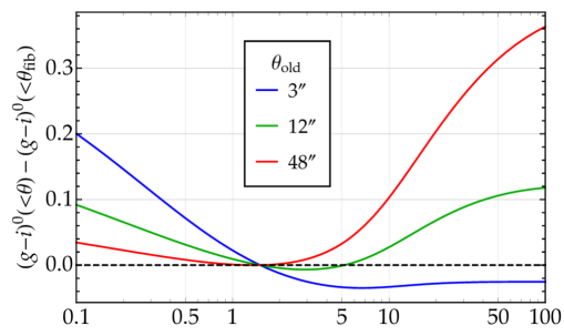
Figure 22: Colour profiles for a mixed population of young and old stars, with $n_{\rm old}=3$ and other parameters from Table 3.

Fig. 22 shows that, contrary to intuition, the mix of a young stellar population with an old one does not necessarily lead to a red colour gradient. This can be understood by the differences in the low and high index Sérsic models: in a log-log plot the surface brightness profile of an $n$=1 Sérsic model is flat in the inner regions and falls rapidly at large radii, while a higher index has a much more gradual decline at all radii. Thus, the high-$n$ Sérsic surface brightness profile dominates the $n$=1 one both at low and high radii. This is similar to spiral galaxies, which are dominated by bulges in their inner regions, spheroids in their outer regions, and with the disc dominating in between. Therefore, the colour of the mix of Sérsic models should have a blue gradient at small radii and a red gradient at large radii. Conversely, the presence of a blue gradient does not necessarily eliminate the possibility of an old, red stellar population at large radii.

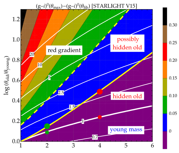
Figure 23: Difference in $(g\!-\!i)^{0}$ colours (eqs. [7]-[9]) between $\theta_{\rm max}=4$ half-light radii of the young population (where SDSS measures the global photometry) and the fibre radius, as a function of the Sérsic index of the old population, $n_{\rm old}$ and the ratio of effective radii $\theta_{\rm old}/\theta_{\rm young}$, assuming the parameters given in Table 3. The solid yellow curve shows the strict upper limit for a blue gradient, while the dashed yellow curve shows the upper limit allowing for a slight red difference of 0.05 magnitudes caused by photometric errors. The white curves indicate the old over young mass ratios, with equality as a thick white curve (as in Fig. 21). The filled circles represent four extreme cases that are discussed for future observability.

Fig. 23 illustrates the difference between the global colour (difference of model magnitudes, measured at $\theta_{\rm max}=4\,\theta_{\rm young}$, because the SDSS photometric pipeline fits exponential profiles out to 4 effective radii) and the fibre colour, again as a function of the old population Sérsic index and of the ratio of old to young effective radii. Fig. 23 clearly shows that there is a range of effective radii of the old population that allows this old population to dominate the total mass (between the thick white curve and either of the yellow curves) without making the colour redder than $(g-i)_{\rm fibre}$. The region between the white and solid yellow curves only allows bluer global colours, while extending to the dashed yellow curve allows slightly redder global colours (by 0.05 mag), consistent with typical photometric errors. For example, if $n_{\rm old}=3$, one can have an old stellar population if $1.5<\theta_{\rm old}/\theta_{\rm young}<2.1$ (i.e. 0.18 to 0.32 in log) for no red gradient, or up to 4.9 for $0<(g-i)^{0}(\theta_{\rm max})-(g-i)^{0}(\theta_{\rm fib})<0.05$, if we allow for photometric errors. The same model applied to the VESPA models, using the same online calculator to recompute the colours and mass-to-light ratios, yields very similar curves as in Fig. 23.

We conclude that forcing a blue gradient does not rule out an underlying old stellar population of high Sérsic index coupled with an effective radius that is greater but not very much greater than that of the young stellar population. Note that in high EW galaxies, the colours are strongly affected by the emission lines, so that bluer does not necessarily mean younger, as is clear in I Zw 18 (Papaderos&Ostlin12). This reinforces the possibility of an old stellar population hiding in our conservative sample of VYGs.

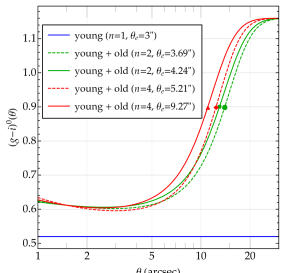
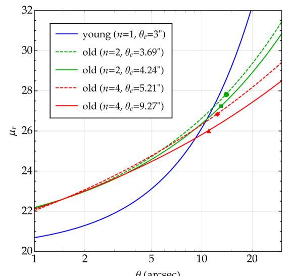
Figure 24: Top: Colour profiles of the young stellar population as well as mixtures of the young with 4 extreme old populations (corresponding to the symbols shown in Fig. 23) that 1) dominate the stellar mass, 2) account for half the stellar mass within the 3 arcsec SDSS fibre, and 3) have a blue gradient. Bottom: Surface brightness profiles for the same models as in the top panel. In both panels, the symbols correspond to $(g-i)^{0}=0.9$, a typical colour that can be distinguished from the bluer inner colour.

We finally ask how deep will observations be required to detect a possible underlying old stellar population. Fig. 24 shows the colour and surface brightness profiles for the young stellar population and mixtures of this young population with four extreme old stellar populations, two with Sérsic index $n_{\rm old}=2$ and two with $n_{\rm old}=4$. For each Sérsic index, we adopt the extreme values for the effective radii, $\theta_{\rm old}$, lying on the thick white (minimum effective radius for old population dominating the mass) and yellow (maximum effective radius to allow for a blue gradient up to $4\,\theta_{\rm young}$) curves of Fig. 23. Assuming 0.1 mag photometric uncertainties for very deep observations, colours will have 0.14 mag uncertainties, and a $2\,\sigma$ detection of a red colour gradient will require a redward shift of 0.3 mag, i.e. an outer colour of $(g-i)^{0}=0.9$ given the typical inner colour of $(g-i)^{0}=0.6$. The top panel of Fig. 24 indicates $(g-i)^{0}=0.9$ is reached between 12 and 15 arcsec. Reading off the corresponding values for the surface brightness in the bottom panel of Fig. 24, we deduce that observations reaching a depth in the range from 26 mag arcsec^-2 ($n_{\rm old}=4$, largest possible $\theta_{\rm old}$) to 28 mag arcsec^-2 ($n_{\rm old}=2$, smallest possible $\theta_{\rm old}$) will be required to detect the possible hidden old stellar population. But Sérsic indices of $n=4$ pertain to giant ellipticals, and a hidden old stellar population is likely to be less luminous and with a lower index, making it more difficult to detect (the surface brightness will need to reach 27 mag arcsec^-2). Repeating this analysis allowing for the $2\,\sigma$ detection of a 0.1 mag redward shift (instead of 0.3 mag) brings the required surface brightness values to 25 to 27 mag arcsec^-2 (26 to 27 mag arcsec^-2 for $n_{\rm old}\leq 3$).

5.9 The number of major starbursts and the reliability of the VYG classification

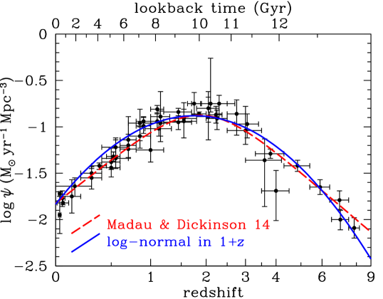
Figure 25: Evolution of the cosmic star formation density. The symbols are the data compiled by Madau & Dickinson (2014), while the dashed red and solid blue curves are two analytical fits from Madau & Dickinson and from our lognormal fit to $\psi$ vs. $1+z$ (with mean of 0.44 and standard deviation 0.21), respectively.

Can the VYG fractions constrain the SFHs of galaxies? The most realistic assumption is that the distribution of lookback times should follow the cosmic star formation history (CSFH). We first note the CSFH (denoted $\psi$) is very close to a log-normal in $1+z$, i.e. $\psi(z)\simeq\psi_{\rm max}\,\exp\{-[\log(1+z)-\mu]^{2}/(2\,\sigma^{2})\}$. This is shown in Figure 25 for our best-fit $\mu=0.44$ and $\sigma=0.21$ (with a peak CSFR $\psi=0.13\rm\,M_{\odot}\,yr^{-1}\,Mpc^{-3}$ at $z=10^{0.44}-1=1.76$, with 84 per cent of the CSFR occurring at redshifts $0.7<z<3.5$). The lognormal CSFH produces a slightly smaller $\chi^{2}$ (in $\log\psi$) than the fit of Madau&Dickinson14, despite having one less parameter (leading to a reduced $\chi_{\nu}^{2}$ of 1.46 instead of 1.58).

The mean redshift of our complete sample is $z_{\rm obs}=0.07$, i.e. a lookback time of 0.93 Gyr. This means that the critical (maximum) redshift for our galaxies to be VYGs is the redshift corresponding to lookback time of 1.93 Gyr, i.e. $z_{\rm crit}=0.154$. According to the lognormal CSFH, we expect the probability $p_{\rm young}$ that a star in a galaxy at $z=0.07$ is younger than 1 Gyr will be

$$p_{\rm young} \!\!\!\!=\!\!\!\! P(z_{\rm obs}<z<z_{\rm crit}\,|\,z>z_{\rm obs})$$ (10)

$$\!\!\!\!=\!\!\!\! {\int_{z_{\rm obs}}^{z_{\rm crit}}\psi(z)\,/\,[(1+z)\,E(z)]\,{\rm d}z\over\int_{z_{\rm obs}}^{\infty}\psi(z)\,/\,[(1+z)\,E(z)]\,{\rm d}z}=0.026\ .$$

In one extreme situation, suppose that all galaxies have single burst SFHs. If we draw random SF redshifts from our lognormal CSFH, we expect that VYGs will comprise 2.6 per cent of our sample of $z=0.07$ galaxies (eq. [10]). At the other extreme, if the SFH of galaxies is continuous, the probability of $>10^{8}$ (unrelated) stars to be younger than 1 Gyr, will be negligible. More precisely, if each star has a probability $p_{\rm young}$ of being younger than 1 Gyr, the probability of $N$ unrelated stars or starbursts (of equal mass) leading to at least half the stellar mass being younger than 1 Gyr will be the cumulative distribution function of the binomial distribution

$$f_{\rm young}=\sum_{k=k_{\rm min}}^{N}{N\choose k}\,p_{\rm young}^{k}\left(1-p_{\rm young}\right)^{N-k}\ ,$$ (11)

where $k_{\rm min}=N/2$ and $(N+1)/2$ for even and odd $N$, respectively. As shown in Figure 26 (symbols), Eq. (11) yields a VYG fraction of $2\,p_{\rm young}\,(1-p_{\rm young}/2)=5$ per cent for $N=2$ starbursts, but falls very rapidly to 0.4 per cent for $N=4$ starbursts, $3\times 10^{-4}$ for $N=6$ starbursts (and below $10^{-10}$ for $N=20$ bursts of SF).

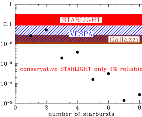
Figure 26: Comparison of prediction of mean fractions of very young galaxies of stellar mass $m>10^{8}{\rm M_{\odot}}$: predicted by the cosmic star formation history (from eq. [11], filled circles) and obtained from SDSS (from eq. [12], shaded regions extending from conservative to liberal).

We compare these predicted VYG fractions with the mean fractions predicted from a mass-limited sample:

$$\left\langle f_{\rm young}\right\rangle={\int_{m_{\rm min}}^{\infty}\phi(m)\,f_{\rm young}(m)\,{\rm d}m\over\int_{m_{\rm min}}^{\infty}\phi(m)\,{\rm d}m}\ ,$$ (12)

where $f_{\rm young}(m)$ is the VYG fraction that we obtained for the complete SDSS/MGS sample and $\phi(m)$ is the $z=0.07$ cosmic stellar mass function. Adopting the double Schechter stellar mass function of Baldry+08 and integrating down to minimum galaxy stellar mass $m_{\rm min}=10^{8}\,{\rm M_{\odot}}$, we find liberal mean VYG fractions of 32, 9 and 3 per cent for STARLIGHT V15, VESPA and Gallazzi, respectively, and conservative fractions of 8 per cent for STARLIGHT V15 and 1 per cent for the VESPA and Gallazzi models, as shown in Figure 26 (shaded regions). The geometric means of these liberal and conservative mean VYG fractions are 16, 3, and 2 per cent for per cent with the STARLIGHT, VESPA, and Gallazzi models, respectively. The VYG classification with STARLIGHT is, at best, 30 per cent reliable for the 2-burst model ($f_{\rm young}=0.05$), while with the other spectral models it is either incomplete and fully reliable for the 2-burst model, or nearly complete and reliable for the single-burst model. For 4 major starbursts, the VYG classification would have reliability of only 2.5, 13 and 20 percent for STARLIGHT, VESPA and Gallazzi, respectively. We now focus on STARLIGHT, which predicts $\sim$ 8 times more frequent conservative VYGs than the other two models. Adopting the ansatz that the conservative VYG classification of STARLIGHT is only 1 per cent reliable, we deduce that $m>10^{8}\rm M_{\odot}$ galaxies undergo on average at most 4 major starbursts.

This discussion is based on the full galaxy population. It cannot be applied to specific populations. It suggests that the decrease of the fraction of VYGs with increasing galaxy stellar mass is a natural outcome of the more bursty SFHs of low mass galaxies (as seen in cosmological hydrodynamical simulations, e.g. Tollet+19).

5.10 Concluding remarks

Our galaxy SFHs from SDSS spectra using different spectral models all indicate that the fraction of VYGs decrease with stellar mass. Nevertheless, the fraction of VYGs remains an unsolved problem for two reasons: 1) the wide variation in estimates of VYG fractions, both among the spectral models, and among the galaxy formation models; 2) the possibility of our missing old stellar populations. Turning this around, we believe that the very strong sensitivity of the fraction of VYGs, to the galaxy formation modelling on one hand (and the number of major starbursts per galaxy) and to the spectral modelling of observed spectra on the other hand, make the study of the mass variation of the fraction of VYGs a strong constraint for both models of galaxy formation and evolution and for spectral models.

It will be worthwhile to confirm the existence of VYGs (some nearly as massive than our Milky Way), in several ways:

1. Analyze the spectra of the VYG candidates with Bayesian modelling (e.g. BEAGLE, Chevallard&Charlot16), for example to penalise against decreasing metal histories.

2. Perform spectral fits to stacked spectra of VYG candidates.

3. Analyze jointly SDSS spectra and photometry in the far- and near-UV from the Galaxy Evolution Explorer (GALEX) and in the near-IR from the Wide-field Infrared Survey Explorer (WISE), accounting for aperture effects (e.g. with BEAGLE).

4. Obtain integral field spectroscopy of a large statistical sample of the VYG candidates to test whether they are globally young or if their youth is restricted to their inner regions probed by the SDSS fibres (instead of relying on the blue colour gradient as a way to avoid aperture effects, since the presence of such a gradient is insufficient to exclude old stellar populations).

5. Obtain deep images of VYG candidates, e.g. with E-ELT, to search for low-surface brightness, extended old stellar populations that may dominate the stellar mass (as Papaderos+02 have done for I Zw 18).

6. Stack hundreds or thousands of images of VYG candidates to achieve comparable depths to search for old stellar populations..

7. Obtain deep near-IR images of nearby VYG candidates with the future James Web Space Telescope (JWST) to derive colour-magnitude diagrams of resolved stars deeper than previously done with HST.

While we cannot be certain that the majority of the thousands of VYGs that we find in the SDSS MGS truly have median ages below 1 Gyr, these VYGs may still hold clues to important recent star formation. Indeed, in a forthcoming article (Trevisan et al. in prep.), we will highlight the specific properties that distinguish VYGs from other star forming galaxies and discuss the impact of galaxy mergers in the formation of VYGs at low redshift. Moreover, we have begun radio observations at GMRT and VLA to understand the kinematics and accretion history of neutral gas around VYGs.

An electronic table of the Clean sample of 404 931 galaxies that are VYGs according to one of our 3 preferred spectral models is provided in electronic form, with the top 10 lines shown in Table 4.

Appendix A Table of very young galaxies

Table 4: Table of Clean sample of 404 931 galaxies that are very young according to at least one of our three preferred spectral models

ID	RA	Dec	plate	MJD	fiber	Compl.	blue	AGN	$\log(m/{\rm M_{\odot}})$	age50 (Gyr)		$\log(m/{\rm M_{\odot}})$	age50 (Gyr)		$\log(m/{\rm M_{\odot}})$	age50 (Gyr)		SFH (SL V15 - no evol)				SFH (SL V15 - evol)
	deg J2000					gradient			SL V15			VESPA BC03			VESPA M05			0–1 Gyr	1–6.1 Gyr	$>$6.1 Gyr		0–1 Gyr	1–6.1 Gyr	$>$6.1 Gyr
(1)	(2)	(3)	(4)	(5)	(6)	(7)	(8)	(9)	(10)	(11)		(12)	(13)		(14)	(15)		(16)	(17)	(18)		(19)	(20)	(21)
1	0.0065	$-0.0926$	387	51791	186	Y	N	T	10.96	5.84		10.67	10.33		10.70	11.43		0.00	0.56	0.44		0.00	0.57	0.43
2	0.0083	$15.6972$	750	52235	456	Y	Y	T	11.04	6.58		10.91	9.44		10.63	7.06		0.01	0.43	0.56		0.01	0.45	0.54
3	0.0087	$15.8817$	750	52235	459	Y	Y	N	10.05	12.93		10.20	3.28		10.25	11.33		0.08	0.04	0.89		0.12	0.04	0.83
4	0.0118	$14.7155$	750	52235	174	N	N	N	9.62	1.36		9.63	3.31		9.66	2.74		0.42	0.36	0.21		0.51	0.34	0.15
5	0.0134	$-1.1130$	685	52203	232	N	Y	N	8.75	0.79		8.92	7.23		8.74	2.67		0.95	0.04	0.01		0.96	0.03	0.01
6	0.0139	$-10.7211$	650	52143	211	Y	Y	T	11.78	12.00		10.99	5.12		10.91	8.19		0.01	0.18	0.81		0.01	0.20	0.79
7	0.0144	$14.1982$	750	52235	92	Y	Y	T	11.61	7.43		11.23	9.61		11.17	9.07		0.01	0.38	0.61		0.01	0.42	0.57
8	0.0174	$-8.7342$	650	52143	446	Y	Y	T	11.27	9.31		10.95	10.89		10.83	7.05		0.00	0.21	0.79		0.00	0.22	0.78
9	0.0192	$-8.9438$	650	52143	447	N	Y	N	8.70	0.47		9.31	5.35		8.82	3.89		0.74	0.26	0.00		0.79	0.21	0.00
10	0.0198	$0.7817$	387	51791	446	Y	Y	T	11.92	8.64		11.53	11.24		11.57	11.09		0.00	0.21	0.79		0.00	0.22	0.77

Notes: the columns are: (1): unique identifier; (2) and (3): equatorial coordinates; (4), (5) and (6): SDSS plate, MJD and fiber; (7): is galaxy in complete sample? (8): does galaxy have a blue colour gradient? ($(g-i)_{\rm model}^{0}<(g-i)_{\rm fiber}^{0}$); (9): is galaxy an AGN: ‘Y’ (yes, above Kewley+01 curve), ‘T’ (transition between curves of Kewley+01 and Kauffmann+03), ‘N’ (no, below Kauffmann+03 curve); (10): stellar mass according to STARLIGHT with V15 model; (11): median age according to STARLIGHT with V15 model; (12): stellar mass according to VESPA with BC03 2-component dust model; (13): median age according to VESPA with BC03 2-component model; (14): stellar mass according to VESPA with M05 2-component dust model; (15): median age according to VESPA with M05 2-component model; (16) to (18): star formation history in respective bins of 0-1 Gyr, 1-6.12 Gyr, and over 6.12 Gyr, using STARLIGHT with the V15 model, with no correction for stellar evolution; (19) to (21): star formation history in respective bins of 0-1 Gyr, 1-6.12 Gyr, and over 6.12 Gyr, using STARLIGHT with the V15 model, now correcting for stellar evolution. The full table for the 404 931 galaxies of the clean sample is available online.