Wave scattering on lattice structures involving array of cracks

Abstract

Scattering of waves due to a vertical array of equally-spaced cracks on a square lattice is studied. The convenience of Floquet periodicity reduces the study to that of scattering of specific wave-mode from single crack in a waveguide. The discrete Green’s function, for the waveguide, is used to obtain semi-analytical solution for scattering problem in case of finite cracks whereas the limiting case of semi-infinite cracks is tackled by an application of Wiener–Hopf technique. Reflectance and transmittance of such an array of cracks, in terms of incident wave parameters, is analyzed. Potential applications include construction of tunable atomic scale interfaces to control energy transmission at different frequencies.

Introduction

Multiple scattering [martinbook] has been researched for more than a century and continues to pose interesting questions, while simultaneously finding applications (see eg., [julius], etc.). In the context of mechanics of solids, presence of defects such as cracks, grooves, holes, etc, [achenbook, julius], lead to scattering of elastic waves. One of the simplest case occurs for scattering of time harmonic anti-plane shear waves as it often allows an analytical investigation [achenbook]; typically, involving two dimensional Helmholtz equation and the prescription of Dirichlet or Neumann condition on certain boundary. Same equation also occurs in special situations dealing with acoustic and electromagnetic waves. Recall that the scattering of H- or E-polarised electromagnetic wave by an infinite array of parallel plates was originally formulated and solved by Carlson and Heins [HeinsI, HeinsII, HeinsIII]. In mechanical framework too, such problems have been studied (see [angelI, kentplates, grating, screens], and references therein), for instance, scattering due to array of cracks.

In recent years, with advancements in technology, the size of structures has been reduced to a few micrometres or nanometres. In a simplified setting, such structures can be modelled using discrete framework [slepyan, brill] which has been around for a while [Lifshitz1, mara]; in fact, some primitive aspects of such models can be traced back to Newton and Hamilton. The discrete models have been extensively used to study brittle fracture [thomson1971lattice, slepyananti, marder, slepyan, marder1], and recently in a series of articles on discrete scattering [sK, sFK, sC, sFC, sWaveguide] in different geometries [sMixed, BGpair1, gmtwocracksasymp]. In this framework, a discrete analogue of the boundary conditions [sK, sC] in the continuous case, depending on the nature of the defects, need to be invoked. For example, a crack [sK, sFK] is modelled by assuming broken bonds between two consecutive rows [slepyananti, slepyan].

The present article follows upon the work of Carlson and Heins [HeinsI, HeinsII, HeinsIII], in the arena of discrete models, as wave scattering due to finite as well as semi-infinite cracks is investigated; the latter employs the method of Wiener and Hopf [noble]. From the viewpoint of applications, the wave transmission across a periodic arrangement of cracks finds potential relevance in radio frequency devices [yang2015II, yang2015I, yang2016]. In certain systems [shin2015], such phononic crystals enable the tailorability, controllability and high conversion efficiency at large frequencies.

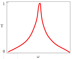
Figure 1: A narrow band of frequency transmitted by the system proposed by [shin2015].

Although, the recently reported transmission behaviour [shin2015] (particularly, a narrow transmission band, shown in the schematic of Fig. 1) is different from the one analyzed in the present work, the geometric arrangements of the cracks allows a favourable transmission/blocking of high frequency lattice waves. In the context of thermal conduction in nano-structures [anufriev2017, li2015], the phonon transmission and reflection has been found to be appropriately controlled using a periodic arrangement of discrete scatterers (air holes, typically). The present study does not investigate any mechanisms enabling the transduction between photons and phonons or the details of phonon transport in monolayers [yang2015I, yang2015II, yang2016, huang2017, xu2018].

In this article, §1 provides the lattice model. §2 formulates the scattering due to a single crack on a lattice ‘waveguide’ and presents the semi-analytical solution for finite crack; the elementary details of calculation of suitable Green’s function are included. The exact solution for semi-infinite case is given in §3, whereas §LABEL:numresult provides some key results and relevant discussion overall. Concluding remarks, and three appendices appear at the end of article.

1 Square lattice model

Consider an infinite square lattice, with each particle of unit mass and an interaction with its four nearest neighbours through linearly elastic identical, massless bonds with a spring constant $1/b^{2}$ [sK] (see Fig. 2(a)). Let $\mathbb{Z}$ denote the set of integers, let $\mathbb{Z}^{2}$ denote $\mathbb{Z}\times\mathbb{Z}$. The lattice contains an infinite array of finite-length cracks (of length $\mathtt{N}_{b}$, i.e., the number of broken bonds) described by the crack faces

$$\{(x,y)\in\mathbb{Z}^{2}|-\mathtt{N}_{b}+n\mathtt{M}\leq x\leq-1+n\mathtt{M},y=n\mathtt{N}+\aleph\,\text{or}\,y=n\mathtt{N}+\aleph-1,n\in\mathbb{Z}\},$$ (2)

where $\mathtt{N}_{b}\in\mathbb{Z}$, $\mathtt{M}\in\mathbb{Z}^{+}$, and $\mathtt{N}\in\mathbb{Z}^{+}$ with (no loss of generality)

$$\aleph={\mathtt{N}/2\text{ when $\mathtt{N}$ is even whereas }\aleph=(\mathtt{N}-1)/2\text{ when $\mathtt{N}$ is odd}.}$$ (3)

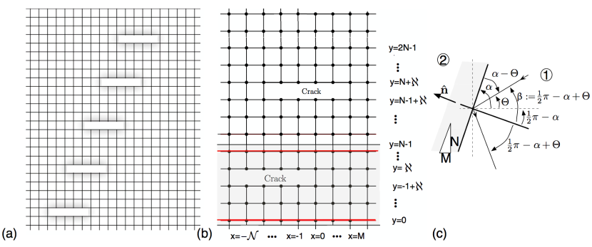
Figure 2: (a) Schematic of lattice with an infinite array of finite, staggered cracks (with $\mathtt{N}_{b}=4,\mathtt{N}=5,\mathtt{M}=2$). (b) The shaded portion (within red lines) corresponds to lattice waveguide containing a single crack. (c) Typical angles.

Suppose $u^{i}$ describes the incident lattice wave with frequency $\upomega$ and a wavenumber $\upkappa$ which is incident on the lattice at an angle $\Theta\in(-\pi,\pi]$. The total displacement $u^{t}$ of a particle satisfies the discrete Helmholtz equation [sK]

$$\Delta u^{t}_{x,y}+\upomega^{2}u^{t}_{x,y}=0,$$ (4)

away from the crack faces (2), with $\Delta u_{x,y}=u_{x+1,y}+u_{x-1,y}+u_{x,y+1}+u_{x,y-1}-4u_{x,y}$. Specifically, it is assumed that (in terms of the incident angle $\Theta$ and incident wavenumber $\upkappa$)

$$u^{i}_{x,y}={{\mathrm{A}}}~{}{\exp}({-i\upkappa x\cos\Theta-i\upkappa y\sin\Theta-ib^{-1}\upomega t}),~{}(x,y)\in\mathbb{Z}^{2},$$ (5)

where ${{\mathrm{A}}}\in\mathbb{C}$. Throughout the article, $\mathbb{C}$ denotes the set of complex numbers, the real part, $\operatorname{\text{\rm Re}}{z}$, of a complex number $z\in\mathbb{C}$ is denoted by $z_{1}$, and its imaginary part, $\operatorname{\text{\rm Im}}{z}$, is denoted by $z_{2}$ (so that $z=z_{1}+iz_{2}$); $|z|$ denotes the modulus for $z\in\mathbb{C}$ while $\arg z$ denotes the argument for $z\in\mathbb{C}$. With schematic illustration in Fig. 2(c), using the reference to the lattice structure shown in Fig. 2(a,b), let ${\upalpha}$ denote the angle of stagger of the crack array (2) relative to the ${x}$ axis, i.e. tanα=N/M, whereas β:= π/2-α+Θ; here, ${\upbeta}$ is the angle of incidence relative to the outward normal to the ‘line’ of the edges. Accordingly, the angle of incidence with respect to the upper side of the edge plane is ${\upalpha}-{\Theta}$.

Substituting (5) in (4) (for an intact lattice), a relation for the triplet $\upomega$, $\upkappa$, $\Theta$, called the dispersion relation (see [sC]), is obtained; it is given by $\upomega^{2}=4\sin^{2}(\frac{1}{2}\upkappa\cos\Theta)+4\sin^{2}(\frac{1}{2}\upkappa\sin\Theta).$ For convenience, a vanishing amount of damping is introduced in the model as in [noble], therefore,

$$\upomega=\upomega_{1}+i\upomega_{2},\upomega_{2}>0.$$ (6)

Thus, $\upkappa$ is also a complex, $\upkappa=\upkappa_{1}+i\upkappa_{2},\upkappa_{2}>0$ (typically, we consider $\upomega_{2}\to 0^{+}$, $\upkappa_{2}\to 0^{+}$). In this article, the scattered wave displacement $u$ is defined as the difference between the total displacement $u^{t}$ and the incident wave displacement $u^{i}$ of an arbitrary particle on the lattice:

$$u_{x,y}=u_{x,y}^{t}-u_{x,y}^{i},~{}~{}(x,y)\in\mathbb{Z}^{2}.$$ (7)

Following [sK, sFK], for a particular crack (say, between $y=\aleph+n\mathtt{N}$ and $y=\aleph-1+n\mathtt{N}$, when $\aleph$ is given by (3) while $n$ is an arbitrary integer), the force in the vertical bonds connecting the particles at $y=\aleph+n\mathtt{N}$ and $y=\aleph-1+n\mathtt{N}$, ahead of the crack, is defined by v_x^t(n):=-1b2v_x^t(n), x∈Z∖{-1+nM,…,-N_b+nM}, with  v_x^t(n):=u^t_x,ℵ+nN-u^t_x,ℵ-1+nN. The force on the particle at $(x,\aleph+n\mathtt{N})$, $x\not\in\{-1+n\mathtt{M},\dotsc,-\mathtt{N}_{b}+n\mathtt{M}\}$, due to the vertical bond with $(x,\aleph-1+n\mathtt{N})$, is $v_{x}^{t}(n)$, while that the force at $(x,\aleph-1+n\mathtt{N})$ due to the same bond is $-v_{x}^{t}(n)$. Since the crack is modelled by assuming broken bonds between two consecutive lattice rows, $v_{x}^{t}(n)=0,~{}~{}x\in\{-1+n\mathtt{M},\dotsc,-\mathtt{N}_{b}+n\mathtt{M}\}.$ It is also useful to define the difference of the scattered displacements, $u_{x,\aleph+n\mathtt{N}}$ and $u_{x,\aleph-1+n\mathtt{N}}$ as

$$\mathtt{v}_{x}(n)=u_{x,\aleph+n\mathtt{N}}-u_{x,\aleph-1+n\mathtt{N}},~{}~{}x\in\mathbb{Z}.$$ (8)

In analogy with (7), a part of the force $v_{x}^{t}(n)$ occurs due to the scattered displacement of particles at $(x,\aleph+n\mathtt{N})$, $x\not\in\{-1+n\mathtt{M},\dotsc,-\mathtt{N}_{b}+n\mathtt{M}\}$; this is given by $v_{x}(n)=-(1/b^{2})\mathtt{v}_{x}(n)$. Let the incident crack opening displacement at $(x,\aleph)$ and $(x,\aleph-1)$, be denoted by

$$\mathtt{v}_{x}^{i}(n)=u_{x,\aleph+n\mathtt{N}}^{i}-u_{x,\aleph-1+n\mathtt{N}}^{i}.$$ (9)

Then, $v_{x}^{i}(n)=-(1/b^{2})\mathtt{v}_{x}^{i}(n)$ can be interpreted as an ‘external force’ on particle at $(x,\aleph+n\mathtt{N})$, $x\in\{-1+n\mathtt{M},\dotsc,-\mathtt{N}_{b}+n\mathtt{M}\}$.

By the virtue of (4), (5) and (7) the scattered wave field also satisfies the discrete Helmholtz equation (4) (replace $u^{t}$ by $u$) away from the array of cracks. The displacement field on the crack face at $y=\aleph+n\mathtt{N}$ and $y=\aleph-1+n\mathtt{N}$ satisfies, respectively,

$$u_{x+1,\aleph+n\mathtt{N}}+u_{x-1,\aleph+n\mathtt{N}}+u_{x,\aleph+1+n\mathtt{N}}+(\upomega^{2}-3)u_{x,\aleph+n\mathtt{N}}=-\mathtt{v}_{x}^{i}(n),$$ (10)

$$u_{x+1,\aleph-1+n\mathtt{N}}+u_{x-1,\aleph-1+n\mathtt{N}}+u_{x,\aleph-2+n\mathtt{N}}+(\upomega^{2}-3)u_{x,\aleph-1+n\mathtt{N}}=\mathtt{v}_{x}^{i}(n),$$ (11)

for $x\in\{-1+n\mathtt{M},\dotsc,-\mathtt{N}_{b}+n\mathtt{M}\}$. Here (10) and (11) can be interpreted as boundary conditions for (4). Then, using the definition of the scattered field $u$, (7), along with the definitions of $\mathtt{v}_{x}(n)$ and $\mathtt{v}_{x}^{i}(n)$ and the boundary conditions (10), (11), the linear difference equation [levy] formally satisfied by the scattered displacement $u$ is

$$\Delta u_{x,y}+\upomega^{2}u_{x,y}=-\sum\nolimits_{n=-\infty}^{\infty}\sum\nolimits_{l=-\mathtt{N}_{b}}^{-1}(\mathtt{v}_{l}(n)+\mathtt{v}_{l}^{i}(n))\delta_{l+n\mathtt{M},x}(\delta_{\aleph+n\mathtt{N},y}-\delta_{\aleph-1+n\mathtt{N},y}),$$ (12)

where $\{\mathtt{v}_{l}(n)\}_{l=-\mathtt{N}_{b},\dotsc,-1;n\in{\mathbb{Z}}}$ are an infinite number of unknowns. Throughout this article, the symbol $\delta$ denotes the Kronecker delta so that $\delta_{a,b}$ equals $0$ if $a\neq b$ while it equals $1$ if $a=b$.

2 Reduction to lattice waveguide with ‘Floquet boundary’: Green’s function and solution for finite cracks

Since the array of finite-length cracks extends indefinitely, there is a periodicity induced into the system by virtue of the Floquet–Bloch theorem. This conveniently reduces the scattering problem to the study of scattering of the incident wave (5) by a single crack in a subset ${\mathscr{S}}_{0}$ (defined below) with $\mathtt{N}$ rows (see the shaded region of Fig. 2(b)). Suppose the region ${\mathscr{S}}_{0}$ corresponds to the crack $n=0$ in (2). Henceforth, in the context of the symbols used for crack opening displacement, $(n)$ notation is dropped; $(0)$ will be omitted for making reference to ${\mathscr{S}}_{0}$. Thus, a shorter notation and Floquet–Bloch periodicity based reduction allows a simplification from the system of equations (12) to the following equation

$$\Delta u_{x,y}+\upomega^{2}u_{x,y}=-\sum\nolimits_{l=-\mathtt{N}_{b}}^{-1}(\mathtt{v}_{l}+\mathtt{v}_{l}^{i})\delta_{l,x}(\delta_{\aleph,y}-\delta_{\aleph-1,y}),(x,y)\in{\mathscr{S}}_{0}.$$ (13)

Observe that the set ${\mathscr{S}}_{0}$ of lattice sites is infinite in the horizontal direction while it is confined in the vertical direction. We employ the natural notation ${\mathbb{Z}}_{a}^{b}$ for the set $\{a,a+1,\dotsc,b\}$ ($\subset{\mathbb{Z}}$). Indeed, $\cup_{n\in{\mathbb{Z}}}{\mathscr{S}}_{n}={\mathbb{Z}^{2}}\text{ with }{\mathscr{S}}_{n}={\mathscr{S}}_{0}+n{\mathtt{N}}\hat{\mathbf{j}}=\{({x},{y}+n{\mathtt{N}})\in{{\mathbb{Z}^{2}}}:{x}\in{\mathbb{Z}},{y}\in{\mathbb{Z}}_{0}^{{\mathtt{N}}-1}\}.$

The incident lattice wave (5), i.e., $u_{x,y}^{i}={{\mathrm{A}}}\exp({-i\upkappa(x\cos\Theta+y\sin\Theta)})$ in ${\mathscr{S}}_{n}$, i.e., at one set of $\mathtt{N}$ rows, in the lattice is related to another set ${\mathscr{S}}_{n+1}$ via

$$u_{x+\mathtt{M},y+\mathtt{N}}^{i}={{\uppsi}}u_{x,y}^{i},\text{where }{{\uppsi}}={\exp}({-i\upkappa(\mathtt{M}\cos\Theta+\mathtt{N}\sin\Theta)}).$$ (14)

By the Floquet–Bloch theorem, the scattered wave field must satisfy identical condition u_x+M, y+N&=ψu_x, y. In the perspective of the infinite square lattice, the formal definition of ${\mathscr{S}}_{0}$ is

$$\{(x,y)\in\mathbb{Z}^{2}|y\in{\mathbb{Z}}_{0}^{{\mathtt{N}}-1},u_{x+\mathtt{M},y+\mathtt{N}}={{\uppsi}}u_{x,y}\}.$$ (15)

Notably ${\mathscr{S}}_{0}$ includes the ‘Floquet’ periodic boundary conditions inherently. The periodically repeating cell (as ${\mathscr{S}}_{n}$s are copies of ${\mathscr{S}}_{0}$) is the ‘waveguide’ mentioned earlier.

Classically, the wave field in a scattering problem can be written in terms of an appropriate Green’s function (see for example, [achenbook]). It has been shown that using discrete Fourier transforms [sFK] a discrete Green’s function (following the traditional terminology), can be also used for the lattice wave scattering. In the present case, the discrete Green’s function $\mathcal{G}$ is sought for the lattice waveguide ${\mathscr{S}}_{0}$ and it satisfies a difference equation given by

$$\Delta\mathcal{G}_{x,y}+\upomega^{2}\mathcal{G}_{x,y}=\delta_{x_{0},x}\delta_{y_{0},y},~{}~{}(x,y)\in{\mathscr{S}}_{0},$$ (16)

where it is assumed that a source is located at $(x_{0},y_{0})\in{\mathscr{S}}_{0}$. Due to (6), note that the Green’s function $\mathcal{G}_{x,y}\sim{\exp}({-\upkappa_{2}|x|})$ as $|x|\to\infty$. The Green’s function, the subject of the following, must satisfy the Floquet periodic boundary conditions of the waveguide. Thus, the difference equation (16) is subjected to the condition (using (14) and (2)) $\mathcal{G}_{x+\mathtt{M},y+\mathtt{N}}={{\uppsi}}\mathcal{G}_{x,y},(x,y)\in{\mathscr{S}}_{0}.$ For the particles at the boundary rows, i.e., at $y=0$ and $y=\mathtt{N}-1$, this leads to $\mathcal{G}_{x+\mathtt{M},\mathtt{N}}={{\uppsi}}\mathcal{G}_{x,0},x\in\mathbb{Z},$ and $\mathcal{G}_{x+\mathtt{M},\mathtt{N}-1}={{\uppsi}}\mathcal{G}_{x,-1},x\in\mathbb{Z},$ respectively. Using (16), the governing equation for a particle at the boundary of the waveguide (that is, $y=0$ and $y=\mathtt{N}-1$, respectively) can be written as

$$\mathcal{G}_{x+1,0}+\mathcal{G}_{x-1,0}+\mathcal{G}_{x,1}+{{\uppsi}}^{-1}\mathcal{G}_{x+\mathtt{M},\mathtt{N}-1}+(\upomega^{2}-4)\mathcal{G}_{x,0}=0,~{}x\in\mathbb{Z},$$ (17)

$$\text{and }\mathcal{G}_{x+1,\mathtt{N}-1}+\mathcal{G}_{x-1,\mathtt{N}-1}+\mathcal{G}_{x,\mathtt{N}-2}+{{\uppsi}}\mathcal{G}_{x-\mathtt{M},0}+(\upomega^{2}-4)\mathcal{G}_{x,\mathtt{N}-1}=0,~{}x\in\mathbb{Z}.$$ (18)

Suppose that the discrete Fourier transform of a sequence $\{u_{m}\}_{m\in\mathbb{Z}}$ is denoted by $u^{{\mathrm{F}}}$ and defined by $u^{{\mathrm{F}}}(z)=\sum\nolimits_{m=-\infty}^{+\infty}u_{m}z^{-m}$. Using the discrete Fourier transform (see also [sFK, gmtwocracksasymp]), the transformed Green’s function can be written as (suppressing $z$ dependence for brevity)

$$\mathcal{G}_{y}^{{\mathrm{F}}}=\sum\nolimits_{x=-\infty}^{\infty}\mathcal{G}_{x,y}z^{-x}.$$ (19)

Based on the nature of $\mathcal{G}_{x,y}$ as $|x|\to\infty$, the region of analyticity of above Fourier transform [sWaveguide] can be found to be an annulus ${{\mathscr{A}}}_{g}$ in the complex plane centred at the origin, which is given by ${{\mathscr{A}}}_{g}=\{z\in\mathbb{C}:{\exp}({-\upkappa_{2}})<|z|<{\exp~{}}{\upkappa_{2}}\}.$ The application of the discrete Fourier transform (19) to (16) results into

$$\mathcal{G}_{y}^{{\mathrm{F}}}({\mathpzc{H}}+2)-(\mathcal{G}_{y+1}^{{\mathrm{F}}}+\mathcal{G}_{y-1}^{{\mathrm{F}}})=-z^{-x_{0}}\delta_{y,y_{0}},\text{where }{\mathpzc{H}}=2-z-z^{-1}-\upomega^{2}.$$ (20)

Similarly, the application of the discrete Fourier transform (19) to the boundary conditions, (17) and (18), respectively, yields

$$\mathcal{G}_{0}^{{\mathrm{F}}}({\mathpzc{H}}+2)-(\mathcal{G}_{1}^{{\mathrm{F}}}+{{\uppsi}}^{-1}z^{\mathtt{M}}\mathcal{G}_{\mathtt{N}-1}^{{\mathrm{F}}})=0,\text{and }\mathcal{G}_{\mathtt{N}-1}^{{\mathrm{F}}}({\mathpzc{H}}+2)-(\mathcal{G}_{\mathtt{N}-2}^{{\mathrm{F}}}+{{\uppsi}}z^{-\mathtt{M}}\mathcal{G}_{0}^{{\mathrm{F}}})=0.$$ (21)

Since (20) is a non-homogeneous linear difference equation in $y$ with coefficients independent of $y$, the solution can be written as [levy] $\mathcal{G}_{y}^{{\mathrm{F}}}=\mathcal{G}_{y}^{Fh}+\mathcal{G}_{y}^{{{\mathrm{F}}}nh},$ where $\mathcal{G}_{y}^{{{\mathrm{F}}}h}$ is the solution to the homogeneous equation $\mathcal{G}_{y}^{{{\mathrm{F}}}h}({\mathpzc{H}}+2)-(\mathcal{G}_{y+1}^{{{\mathrm{F}}}h}+\mathcal{G}_{y-1}^{{{\mathrm{F}}}h})=0,$ with certain boundary conditions (to be stated below), and $\mathcal{G}_{y}^{{{\mathrm{F}}}nh}$ is a particular solution of

$$\mathcal{G}_{y}^{{{\mathrm{F}}}nh}({\mathpzc{H}}+2)-(\mathcal{G}_{y+1}^{{{\mathrm{F}}}nh}+\mathcal{G}_{y-1}^{{{\mathrm{F}}}nh})=-\delta_{y,y_{0}}z^{-x_{0}}.$$ (22)

Using elementary calculus [sCheby], a (particular) solution of (22) is found

$$\mathcal{G}_{y}^{{{\mathrm{F}}}nh}=G_{0}(z){{\lambda}}^{|y-y_{0}|}(z),z\in{{\mathscr{A}}},$$ (23)

where [sK, sFK, slepyan] λ(z):=r(z)-h(z)r(z)+h(z), z∈C∖B, h(z):=H(z), r(z):=H(z)+4. The square root function, $\sqrt{\cdot}$, has the branch cut from $-\infty$ to $0$. ${\mathscr{B}}$ denotes the union of branch cuts for ${{\lambda}}$, borne out of the chosen branch for ${{\mathpzc{h}}}$ and ${{\mathpzc{r}}}$ such that $|{{\lambda}}({{z}})|\leq 1,{{z}}\in{\mathbb{C}}\setminus{\mathscr{B}}.$ In above equations, the annulus ${{\mathscr{A}}}$ is given by

$${{\mathscr{A}}}={{\mathscr{A}}}_{g}\cap{{\mathscr{A}}}_{\mathfrak{L}},$$ (24)

with ${{\mathscr{A}}}_{\mathfrak{L}}$ being the annular region where ${\mathpzc{h}}$ and ${\mathpzc{r}}$ (and ${\lambda}$ too) are analytic (for ${\mathscr{A}}_{g}$, see the sentence following (19)). The coefficient $G_{0}$ in (23) is determined by substituting the ansatz of $\mathcal{G}_{y}^{{{\mathrm{F}}}nh}$ in (22), that is, $G_{0}{{\lambda}}^{|y-y_{0}|}({\mathpzc{H}}+2)-(G_{0}{{\lambda}}^{|y-y_{0}+1|}+G_{0}{{\lambda}}^{|y-y_{0}-1|})=-z^{-x_{0}}\delta_{y-y_{0},0},$ for $z\in{{\mathscr{A}}}$, which leads to $G_{0}=-{z^{-x_{0}}}/{({{\mathpzc{H}}+2-2{{\lambda}}})}$, so that, a particular solution of the linear non-homogeneous difference equation (22) can be written as [levy]

$$\mathcal{G}_{y}^{{{\mathrm{F}}}nh}=-\frac{z^{-x_{0}}{{\lambda}}^{|y-y_{0}|}}{{\mathpzc{H}}+2-2{{\lambda}}},z\in{{\mathscr{A}}}.$$ (25)

After substitution of the particular solution (25) of (20) in the boundary conditions (21) (for $y=0$ and $y=\mathtt{N}-1$), we obtain the boundary conditions for the homogenous solution $\mathcal{G}_{y}^{{{\mathrm{F}}}h}$,

$$\mathcal{G}_{0}^{{{\mathrm{F}}}h}({\mathpzc{H}}+2)-(\mathcal{G}_{1}^{{{\mathrm{F}}}h}+z^{\mathtt{M}}{{\uppsi}}^{-1}\mathcal{G}_{\mathtt{N}-1}^{{{\mathrm{F}}}h})=\frac{z^{-x_{0}}({{\lambda}}^{|y_{0}|}({\mathpzc{H}}+2)-{{\lambda}}^{|1-y_{0}|}-{{\lambda}}^{|\mathtt{N}-1-y_{0}|}{{\uppsi}}^{-1}z^{\mathtt{M}})}{{\mathpzc{H}}+2-2{{\lambda}}},$$ (26)

$$\mathcal{G}_{\mathtt{N}-1}^{{{\mathrm{F}}}h}({\mathpzc{H}}+2)-(\mathcal{G}_{\mathtt{N}-2}^{{{\mathrm{F}}}h}+{{\uppsi}}z^{-\mathtt{M}}\mathcal{G}_{0}^{{{\mathrm{F}}}h})=\frac{z^{-x_{0}}({{\lambda}}^{|\mathtt{N}-1-y_{0}|}({\mathpzc{H}}+2)-{{\lambda}}^{|\mathtt{N}-2-y_{0}|}-{{\uppsi}}z^{-\mathtt{M}}{{\lambda}}^{|y_{0}|})}{{\mathpzc{H}}+2-2{{\lambda}}},$$ (27)

for $z\in{{\mathscr{A}}}$ (recall that $\mathpzc{H}$ is defined by (20)); these conditions are used to determine the unknown coefficients in the general solution for homogenous part. After an elementary calculation, we find

$${\mathcal{G}}_{y}^{{\mathrm{F}}}=-z^{-x_{0}}\frac{{{\mathtt{U}}}_{\mathtt{N}-|y-y_{0}|-1}(\vartheta)+{{\mathtt{U}}}_{|y_{0}-y|-1}(\vartheta)({\uppsi}z^{-\mathtt{M}})^{\text{sign}(y-y_{0})}}{2{\mathtt{T}}_{\mathtt{N}}(\vartheta)-({\uppsi}z^{-\mathtt{M}}+{\uppsi}^{-1}z^{\mathtt{M}})},\text{where }\vartheta=1+\frac{1}{2}{\mathpzc{H}}.$$ (28)

It is emphasized that the numerator and denominator in (28) involve the Chebyshev polynomials which have been found significant in the description of wave propagation characteristics of lattice waveguides [sCheby, sHoney]. In particular, ${\mathtt{U}}_{n}$ denotes the Chebyshev polynomials of second kind [mason] defined by ${\mathtt{U}}_{n}(\vartheta):=\sin((n+1)\vartheta)/\sin\vartheta,n\geq 0$ while ${\mathtt{T}}_{n}$ denotes the Chebyshev polynomials of first kind [mason] defined by ${\mathtt{T}}_{n}(\vartheta):=\cos n\vartheta$.

The discrete Green’s function in the physical domain can be obtained by inverse Fourier transform of (28), i.e.,

$$\mathcal{G}_{x,y}=\frac{1}{2\pi i}\oint_{C}\mathcal{G}_{y}^{{\mathrm{F}}}(z)z^{x-1}\,dz,$$ (29)

where $C$ can be chosen to be a closed contour that lies inside the annulus ${{\mathscr{A}}}$ (24). Due to the vanishingly small imaginary part of the frequency and hence, the wavenumber, all the singularities of the integrand in (29), are either inside the unit circle or outside the circle, that is, they are away from the contour (see [noble]). Till this point, our exposition completes the derivation of the discrete Green’s function. It turns out that the denominator of the transformed Green’s function, (28), represents the dispersion relation for a square lattice waveguide with Floquet–Bloch periodic boundaries. Brief discussion of the same is provided in Appendix LABEL:wdisperse.

The description of the scattered displacement field in terms of the Green’s function (29) now follows the well known approach [Lifshitz1] (see also [sFK, sFC] for notation relevant to the manipulations presented below). In fact, the present problem is closely related to the scattering due to a finite crack in infinite lattice and the description of the scattered field $u$ in terms of the Green’s function has been discussed systematically in [sFK]. For additional clarity, $\mathcal{G}_{x,y;x_{0},y_{0}}$ will be used instead of $\mathcal{G}_{x,y}$ in the subsequent paragraphs. Note that the expression (29) is the solution of the equation (16) which has the source located at $(x_{0},y_{0})$ (recall (16)).

Using (13) and (16), by inspection, it can be found that the scattered displacement field due to an infinite array of cracks in the lattice is given by

$$u_{x,y}=-\sum\nolimits_{l=-\mathtt{N}_{b}}^{-1}(\mathtt{v}_{l}+\mathtt{v}_{l}^{i})(\mathcal{G}_{x,y;l,\aleph}-\mathcal{G}_{x,y;l,\aleph-1}),$$ (30)

for $(x,y)\in{\mathscr{S}}_{0}$. In fact, (30) provides the unique solution to the equation (13) in terms of the crack opening displacement $\{\mathtt{v}_{l}\}_{l\in\in{\mathbb{Z}}_{-\mathtt{N}_{b}}^{-1}}$. The rigorous aspects of the issue of existence and uniqueness of the solution, for the assumed case $\upomega_{2}>0$, are analogous to the results provided in [sFK] and are, therefore, omitted in the present article. Substitution of (30) into (8) yields a system of equations of the form

$$\sum\nolimits_{l=-\mathtt{N}_{b}}^{-1}\mathtt{c}_{j,l}\mathtt{v}_{l}=b_{j},~{}~{}j\in{\mathbb{Z}}_{-\mathtt{N}_{b}}^{-1},$$ (31)

$$\text{where }\mathtt{c}_{j,l}=\delta_{j,l}-(-\mathcal{G}_{j,\aleph;l,\aleph}+\mathcal{G}_{j,\aleph;l,\aleph-1}+\mathcal{G}_{j,\aleph-1;l,\aleph}-\mathcal{G}_{j,\aleph-1;l,\aleph-1}),$$ (32)

$$b_{j}=\sum\nolimits_{l=-\mathtt{N}_{b}}^{-1}(\delta_{l,j}-\mathtt{c}_{j,l}),\text{ for }j\in{\mathbb{Z}}_{-\mathtt{N}_{b}}^{-1}.$$ (33)

Introducing $\mathbf{v}=[\mathtt{v}_{-1},\mathtt{v}_{-2},\dotsc,\mathtt{v}_{-\mathtt{N}_{b}}]^{T}\in\mathbb{C}^{\mathtt{N}_{b}}~{}~{}\text{and}~{}~{}\mathbf{v}^{i}=[\mathtt{v}_{-1}^{i},\mathtt{v}_{-2}^{i},\dotsc,\mathtt{v}_{-\mathtt{N}_{b}}^{i}]^{T}\in\mathbb{C}^{\mathtt{N}_{b}},$ (31) can be expressed as $\mathbf{v}=\mathbf{F}_{\mathtt{N}_{b}}(\mathbf{v}+\mathbf{v}^{i})$, where $\mathbf{F}_{\mathtt{N}_{b}}$ is an $\mathtt{N}_{b}\times\mathtt{N}_{b}$ matrix with $[\mathbf{F}_{\mathtt{N}_{b}}]_{j,l}={\delta_{j,l}-\mathtt{c}_{j,l}}$. Therefore, $\mathbf{v}=(\mathbf{I}_{\mathtt{N}_{b}}-\mathbf{F}_{\mathtt{N}_{b}})^{-1}\mathbf{F}_{\mathtt{N}_{b}}\mathbf{v}^{i}.$ The matrix $\mathbf{F}_{\mathtt{N}_{b}}$ is a matrix, of the Toeplitz form [sK, sFK] due to peculiar nature of the Green’s function (16). Eventually, the complete displacement field on the lattice (with an array of cracks) can be written by substitution of the components of $\mathbf{v}$ in (30) and extending to the entire lattice by using the Floquet phase factor (14).

3 Semi-infinite cracks: Wiener–Hopf method

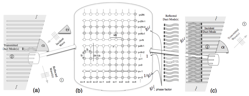
Figure 3: A schematic illustration of an infinite array of cracks with a horizontal stagger ${\mathtt{M}}$ (b), together with directions of incident wave, reflected wave(s), and duct mode(s) in (a) and (c), respective to the incidence from bulk lattice (1) and portion between the cracks (2). The crack tips shown schematically in (b). Intact lattice is shown as gray dots and the particles located at the crack faces (lacking a nearest neighbor bond) as white dots.

In the following, the limiting case as $\mathtt{N}_{b}\to\infty$, i.e. semi-infinite cracks, is analyzed via the method of Wiener and Hopf [noble]. We depart from the choice (3), also without any loss of generality, and consider the choice $\aleph=0$ in the context of (2). The details of the wave propagation problem concerning the periodically repeating cell ${\mathscr{S}}_{0}$ are provided in Appendix LABEL:wdisperseLABEL:appWmodeaway; this is now important for the case of semi-infinite cracks since one possible mode of incidence corresponds to that from the cracked portions (with the assumption that the incidence from the infinite array still satisfies the Floquet condition (14)).

After taking the Fourier transform along ${x}$, the general solution of the discrete Helmholtz equation (4) for the scattered wave field in the lattice sites sandwiched between the two edges of ${\mathscr{S}}_{0}$, i.e., ${y}=0$ and ${y}={\mathtt{N}}-1$, is given by ${u}^{{\mathrm{F}}}_{{y}}=a{\lambda}^{{y}}+b{\lambda}^{-{y}},{y}\in{\mathbb{Z}}_{0}^{{\mathtt{N}}-1},$ where ${\lambda}$ is defined in (23). After solving for $a$ and $b$ in terms of ${u}^{{\mathrm{F}}}_{0},{u}^{{\mathrm{F}}}_{{\mathtt{N}}-1}$, it is easy to see that u^F_y=u^F_0λy-λ2N-2-y1-λ2N-2+u^F_N-1λN-1-y-λN-1+y1-λ2N-2, y∈Z_0^N-1. As observed in the previous section, the phase modulated periodicity (14) implies ${u}^{{\mathrm{F}}}_{{\mathtt{N}}-1}={\uppsi}{z}^{-{\mathtt{M}}}{u}^{{\mathrm{F}}}_{-1}.$ We now consider the discrete Fourier transform as a sum of a pair of half-transforms, u^F(z)=u_+(z)+u_-(z), u_+(z)=∑_m=0^+∞u_mz^-m, u_-(z)=∑_m=-∞^-1u_mz^-m. Employing the discrete Fourier transform (3) to the governing equation for a particle at $y=0$ and $y=-1$, respectively, we get (recall that $\mathpzc{H}$ is defined by (20))

$$-{{b}^{2}}{{\mathit{v}}}^{i}_{0;-}({{z}})+{u}_{0;-}({{z}})-{u}_{-1;-}({{z}})=({{\mathpzc{H}}}({{z}})+2){u}^{{\mathrm{F}}}_{0}({{z}})-{u}_{1}^{{\mathrm{F}}}({{z}})-{u}_{-1}^{{\mathrm{F}}}({{z}}),$$ (34)

$${{b}^{2}}{{\mathit{v}}}^{i}_{0;-}({{z}})+{u}_{-1;-}({{z}})-{u}_{0;-}({{z}})=({{\mathpzc{H}}}({{z}})+2){u}^{{\mathrm{F}}}_{-1}({{z}})-{u}_{-2}^{{\mathrm{F}}}({{z}})-{u}_{0}^{{\mathrm{F}}}({{z}}),{{z}}\in{{{\mathscr{A}}}},$$ (35)

$$\text{where }{{\mathit{v}}}^{i}_{0;-}({{z}})={b}^{-2}{{{\mathrm{A}}}}(1-{\exp}({i{\upkappa}_{y}}))\delta_{D-}({{z}}{{z}}_{{P}}^{-1}),\text{and }\delta_{D-}({{z}}){:=}\sum\nolimits_{n=-\infty}^{-1}{{z}}^{-n},|{{z}}|<1,$$ (36)

$${{z}}_{{P}}{:=}{\exp}({-i{\upkappa}\cos{\Theta}})\in{\mathbb{C}},\text{further, \eqref{floquet} implies ${\uppsi}={z}_{{P}}^{{\mathtt{M}}}{\lambda}_{{P}}^{-{\mathtt{N}}}\text{ with }{\lambda}_{{P}}={\lambda}({z}_{{P}})={\exp}({i{\upkappa}\sin{\Theta}}).$}$$ (37)

In (36)₂, it is clear that $\delta_{D-}({{z}})=z/(1-z)$ (using formula for the geometric series). Using (3) and (14), the pair of coupled Wiener–Hopf equations (35) can be expressed as &B[u0;+u-1;+]+ (B-[1-1-11])[u0;-u-1;-]=[-11]b^2v^i_0;-,
where B=[νN-(1+z-MψμN)-(1+zMψ-1μN)νN], ν_N =λ-N-λNλ1-N-λN-1, μ_N =λ-1-λλ1-N-λN-1. Although above problem (3) appears to be in the realm of matrix Wiener–Hopf kernels [noble], there exists a structure which leads to its reduction to scalar equation. Indeed, after addition of both component equations in (3), it is found that u_-1;++u_-1;-=u_-1^F=Vu_0^F=V(u_0;++u_0;-), where V=-νN-1-μNzMψ-1νN-1-μNz-Mψ. On the other hand, taking the difference of both equations (3) (at this point recall (8)), using v^F=v_++v_-=u_0^F-u_-1^F=(1-V)u_0^F, and simplifying further (following [sWaveguide]), a scalar Wiener–Hopf equation result in ${\mathtt{v}}_{\pm}$, i.e., v_+(z)+L_(z) v_-(z)=-(1-L_(z))b^2v^i_0;-(z),  z∈A, where L_ &=H(z)UN-1(ϑ)2TN(ϑ)-(zMψ-1+z-Mψ)=ND. In fact, by virtue of the presence of Chebyshev polynomials [sCheby] of argument $\vartheta$ (28), an equivalent expression for kernel is ${{\operatorname{\mathpzc{L}}}}={\mathpzc{h}}^{2}\prod_{j=1}^{{\mathtt{N}}-1}({{\mathpzc{h}}}^{2}+4\sin^{2}\frac{1}{2}\frac{j\pi}{{\mathtt{N}}})/\big{(}\prod_{j=1}^{{\mathtt{N}}}({{\mathpzc{h}}}^{2}+4\sin^{2}\frac{1}{2}\frac{(j-\frac{1}{2})\pi}{{\mathtt{N}}})-({z}^{{\mathtt{M}}}{z}_{{P}}^{-{\mathtt{M}}}{\lambda}_{{P}}^{{\mathtt{N}}}+{z}^{-{\mathtt{M}}}{z}_{{P}}^{{\mathtt{M}}}{\lambda}_{{P}}^{-{\mathtt{N}}})\big{)}$; recall that ${\uppsi}$ is defined by (14) and ${\lambda}_{{P}},{z}_{{P}}$ by (37).

The discrete Wiener–Hopf equation (3) has the same form as Eq. (2.23) in [sK] and in fact it is almost identical to (2.8) in [sWaveguide], hence, employing the same kind of, elementary, multiplicative factorization of the kernel ${{\operatorname{\mathpzc{L}}}}$ (following the section §2.4 of [sWaveguide]), i.e., ${\operatorname{\mathpzc{L}}}={\operatorname{\mathpzc{L}}}_{+}{\operatorname{\mathpzc{L}}}_{-}$ on $\mathscr{A}$, we find L^-1_+(z)v_+(z)+L__-(z)v_-(z)=C(z),  z∈A_, where ${{\mathpzc{C}}}({{z}})=({{\operatorname{\mathpzc{L}}}}_{{}+}^{-1}({{z}})-{{{\operatorname{\mathpzc{L}}}}}_{-}({{z}})){{{\mathrm{A}}}}(1-{\exp}({i{\upkappa}_{y}}))\delta_{D-}({{z}}{{z}}_{{P}}^{-1}),{{z}}\in{{{\mathscr{A}}}}.$ Further, an additive factorization of ${{\mathpzc{C}}}$, following [sK], is C=C_+(z)+C_-(z), C_±(z)=∓A(1-exp(i κ_y))(L^-1_+(z_P)-L__±^∓1(z))δ_D-(z z_P^-1),  z∈A_, which leads to the exact solution of (3) as v_±(z)=C_±(z)L__±^±1(z), z∈C, —z—≷$\max$$\min${R_±, R_L_^±1}. Recall that ${z}_{{P}}$ is given by (37).

Using (3), the exact solution (3) implies ($\mathtt{v}^{{\mathrm{F}}}=\mathtt{v}_{+}+\mathtt{v}_{-}$) u