The variability of the star formation rate in galaxies: I. Star formation histories traced by EW(H$\alpha$) and EW(H$\delta_{\rm A}$)

Abstract

To investigate the variability of the star formation rate (SFR) of galaxies, we define a star formation change parameter, ${\rm SFR}_{\rm 5Myr}/{\rm SFR}_{\rm 800Myr}$  which is the ratio of the SFR averaged within the last 5 Myr to the SFR averaged within the last 800 Myr. We show that this parameter can be determined from a combination of H$\alpha$ emission and H$\delta$ absorption, plus the 4000 Å break, with an uncertainty of $\sim$0.07 dex for star-forming galaxies. We then apply this estimator to MaNGA galaxies, both globally within $R_{e}$ and within radial annuli. We find that the global ${\rm SFR}_{\rm 5Myr}/{\rm SFR}_{\rm 800Myr}$, which indicates by how much a galaxy has changed its specific SFR (sSFR) is nearly independent of its sSFR, i.e. of its the position relative to the star formation main sequence (SFMS) as defined by SFR_800Myr. Also, at any sSFR, there are as many galaxies increasing their sSFR as decreasing it, as required if the dispersion in the SFMS is to stay the same. The ${\rm SFR}_{\rm 5Myr}/{\rm SFR}_{\rm 800Myr}$ of the overall galaxy population is very close to that expected for the evolving Main Sequence. Both of these provide a reassuring check on the validity of our calibration of the estimator. We find that galaxies with higher global ${\rm SFR}_{\rm 5Myr}/{\rm SFR}_{\rm 800Myr}$ appear to have higher ${\rm SFR}_{\rm 5Myr}/{\rm SFR}_{\rm 800Myr}$ at all galactic radii, i.e. that galaxies with a recent temporal enhancement in overall SFR have enhanced star formation at all galactic radii. The dispersion of the ${\rm SFR}_{\rm 5Myr}/{\rm SFR}_{\rm 800Myr}$ at a given relative galactic radius and a given stellar mass decreases with the (indirectly inferred) gas depletion time: locations with short gas depletion time appear to undergo bigger variations in their star-formation rates on Gyr or less timescales. In Wang et al. (2019) we showed that the dispersion in star-formation rate surface densities $\Sigma_{\rm SFR}$ in the galaxy population appears to be inversely correlated with the inferred gas depletion timescale and interpreted this in terms of the dynamical response of a gas-regulator system to changes in the gas inflow rate. In this paper, we can now prove directly with ${\rm SFR}_{\rm 5Myr}/{\rm SFR}_{\rm 800Myr}$ that these effects are indeed due to genuine temporal variations in the SFR of individual galaxies on timescales between $10^{7}$ and $10^{9}$ years rather than possibly reflecting intrinsic, non-temporal, differences between different galaxies.

1. Introduction

Studying the star formation histories (SFH) of galaxies is a major tool to study the formation and evolution of galaxies. Thanks to a series of deep surveys of galaxies, the evolution of the star formation rate (SFR) for the global galaxy population also known as the cosmic evolution of the star formation rate density (SFRD), is well established up to redshift of $\sim$9 (e.g. Lilly et al., 1996; Schiminovich et al., 2005; Bouwens et al., 2011, 2014; Madau & Dickinson, 2014; Hagen et al., 2015; Alavi et al., 2016; Goto et al., 2019). The evolution of the SFRD is measured based on the galaxy population at different redshifts.

Observationally, most star-forming (SF) galaxies form a narrow sequence on the stellar mass-SFR diagram up to at least redshift of 3 (e.g. Brinchmann et al., 2004; Daddi et al., 2007; Elbaz et al., 2007; Noeske et al., 2007; Elbaz et al., 2011). This sequence is known as the star formation main sequence (SFMS). The relation is approximately linear, i.e. there is a characteristic specific SFR (sSFR). The sSFR-normalization of the SFMS has been found to evolve with lookback time as $(1+z)^{2.2}$ (Pannella et al., 2009; Stark et al., 2013; Schreiber et al., 2015; Boogaard et al., 2018). This increase with look-back time of the sSFR of typical galaxies at a given mass is due to the higher rate of accretion of cold gas by galaxies at high redshift. The scatter of the SFMS is rather small at any given redshift, 0.2-0.4 dex, depending on the exact definition of the SF populations and the method to obtain the stellar masses and SFRs. The origin of the SFMS and the small scatter of the SFMS is not well understood, but likely reflects the effect of a long-term quasi-steady state between gas accretion, star formation and gas outflow driven by feedback processes (e.g. Schaye et al., 2010; Bouché et al., 2010; Davé et al., 2011; Lilly et al., 2013; Tacchella et al., 2016; Rodríguez-Puebla et al., 2016; Wang et al., 2019).

It is clear that the scatter of the SFMS is relevant to the variability of SFHs of individual SF galaxies, and accurate measurements of SFHs could uncover the contributions of the scatter of SFMS by the variation of SFHs at different timescales. However, the accurate star formation histories of individual galaxies are still poorly determined from observations, especially on short timescales ($<100$ Myr).

Many physical processes have been proposed to account for the variability of the SFHs for individual galaxies. These processes are generally separated into two types: internal processes and those driven by the external environment. Basically, these processes enhance or suppress (or even quench) the star formation by producing changes in the cold gas content and/or a change in the star formation efficiency (SFE), defined as the SFR per unit mass of cold gas. For instance, disk instabilities (e.g. Dekel & Burkert, 2014; Zolotov et al., 2015; Tacchella et al., 2016) and bar-induced gas inflows (e.g. Wang et al., 2012; Lin et al., 2017; Chown et al., 2019) may enhance the star formation via an increase of star formation efficiency, while outflows driven by stellar feedback (e.g. Ceverino & Klypin, 2009; Muratov et al., 2015; El-Badry et al., 2016) or tidal/ram-pressure stripping in massive halos (e.g. Gunn & Gott, 1972; Moore et al., 1996; Abadi et al., 1999; Poggianti et al., 2017) may suppress the star formation in galaxies by removing cold gas.

The variability of SFHs on short and long timescales is likely governed by physical processes operating on different timescales (Sparre et al., 2015, 2017; Broussard et al., 2019; Wang et al., 2019). For instance, variations in gas accretion may drive the variation of SFR on relatively long timescales (Sparre et al., 2015; Wang et al., 2019), while feedback from supernovae or active galactic nuclei (AGN) may produce changes in the SFR on relatively short timescales (Sparre et al., 2017). Having more extensive information of how individual galaxies change their SFRs over time could reveal which physical processes enhance or suppress the star formation during the lifetime of galaxies, and which processes govern the variation of SFR over long and short timescales.

Hydro-dynamical simulations can, in principle, produce accurate SFHs of simulated galaxies, which may be helpful to understand the origin of the scatter of the SFMS, regardless of the poorly understood sub-grid physics. Indeed, based on cosmological zoom-in simulations of 26 moderately massive galaxies, Tacchella et al. (2016) found that SF galaxies oscillate about the SFMS ridge on time-scales of $\sim$0.4 Hubble time ($t_{\rm Hubble}$) at $1<z<4$. The oscillation is the result of an interplay between gas compaction, gas depletion (including star formation and outflow), and accretion. Based on the EAGLE simulations, Matthee & Schaye (2019) investigated the evolution and origin of the scatter of the SFMS. They found that the scatter in sSFR in the local Universe originates in their simulation from a combination of fluctuations on short time-scales (0.2-2 Gyr), likely associated with self-regulation of cooling, star formation and outflows, and variations on long time-scale ($\sim 10$ Gyr) associated to different halo formation times. They found that the long time-scale variations dominate the scatter of the SFMS in the local Universe. Rodríguez-Puebla et al. (2016) found that the scatter of the halo mass accretion rate ($\sim$0.3 dex) in the Bolshoi-Planck simulation (Klypin et al., 2016) is comparable to the observed scatter of SFMS. However, it should be noted that the halo mass accretion rate is averaged over 0.2$t_{\rm Hubble}$, which is much larger than the timescale of most SFR indicators in observations, such as H$\alpha$ and ultraviolet/infrared luminosity. The scatter of halo mass accretion rate could be larger than 0.3 dex if it was averaged within a shorter timescale.

Although the integrated spectral energy distribution (SED) of galaxies records the information of star formation at different lookback times, it is very challenging to obtain accurate SFHs by SED modelling (e.g. Papovich et al., 2001; Shapley et al., 2001; Muzzin et al., 2009; Conroy, 2013; Carnall et al., 2019; Leja et al., 2019). As shown in the SED modelling test of Ge et al. (2018), the SED fitting code is able to reproduce the input stellar population age, metallicity and mass-to-light ratio with reasonable accuracy in dust-poor cases, while large discrepancies can occur in dust-rich cases. In addition, although SED modelling can reproduce the overall shape of input SFHs in most cases, the short-time variations ($\sim 100$ Myr) in SFHs are usually not well recovered (e.g. Ocvirk et al., 2006; Gallazzi & Bell, 2009; Zibetti et al., 2009; Leja et al., 2019). Considering the possible variation of the initial mass function (IMF), and possibly different dust attenuations in young and old stellar populations (Calzetti et al., 2000; Moustakas & Kennicutt, 2006; Wild et al., 2011; Hemmati et al., 2015; Reddy et al., 2015), we are still quite a long way from obtaining accurate SFHs from SED modelling. An alternative way of obtaining individual SFHs is to analyze images of galaxies that are resolved down to individual stars (e.g. Tolstoy et al., 2009; Cignoni et al., 2015; Sacchi et al., 2019), but this approach is only practical for the closest galaxies.

Given the difficulties of obtaining accurate SFHs of galaxies from observations, a number of measures comparing a longer-timescale SFR to a shorter-timescale SFR have been proposed in the literature (Sullivan et al., 2000; Boselli et al., 2009; Wuyts et al., 2011; Guo et al., 2016; Sparre et al., 2017; Broussard et al., 2019; Emami et al., 2019; Faisst et al., 2019). These are often called “burstiness” parameters, but we ourselves find this restrictive, as will be dismissed below. It is clear that such burstiness contains information on the variability of recent SFHs. Weisz et al. (2012) found that the distribution of H$\alpha$-to-far-UV (FUV) flux ratios of a sample of 185 nearby galaxies can be well matched with simple, periodic SFH models, but can not be matched by the constant SFHs with varying IMF. Guo et al. (2016) found a decrease in H$\beta$-to-FUV ratio with decreasing galaxy mass, which can be explained by a bursty SFH on a timescale of a few tens of Myrs on galactic scales. More recently, Broussard et al. (2019) found that the dispersion of burstiness characterizes the stochasticity of a galaxy population’s recent star formation, rather than the average value of burstiness. Consistent with this, Caplar & Tacchella (2019) have tried to use the scatter of the SFMS based on different SFR indicators to model the stochasticity of SFHs.

A common method of quantifying burstiness is to use the average H$\alpha$-to-UV flux ratio. The H$\alpha$ emission is produced by the recombination of gas ionized by photons from massive stars ($>15$${\rm M}_{\odot}$), and is expected to be observed only within the typical lifetimes of these massive stars ($<5$ Myr). The UV continuum comes from non-ionizing photospheric emission from stars with mass greater than 3${\rm M}_{\odot}$ (Kennicutt, 1998, and references therein), which have lifetimes of $<$300 Myr. However, as pointed out by Caplar & Tacchella (2019), the commonly-used SFR indicators, such as H$\alpha$, NUV, FUV, u-band and UV+IR luminosities, do not exactly follow the recent SFHs within a specified timescale. Instead, the SFRs traced by any of these indicators can be considered to be a convolution of the SFH with the luminosity evolution of these indicators for a single stellar population. This increases the complexity of studying the stochasticity of SFHs of a galaxy population. In addition, the measured burstiness based on the above indicators strongly depends on the dust attenuation correction, which may significantly broaden the scatter.

In this work, we develop a new parameter to characterize the change of star formation, SFR_5Myr/SFR_800Myr. This is the ratio of the SFR averaged within the most recent 5 Myr to the SFR averaged within the last 800 Myr. The definition of this parameter is similar to the definition of the burstiness in the literature, but in this work we prefer to call it a “star formation change parameter” (or simply the “change parameter”), because galaxies can either enhance or suppress their star formation in the recent 5 Myr with respect to the average star formation within the last 800 Myr. In other words, the parameter can take values above or below unity, and indeed should average to unity over a large enough population.

Our change parameter SFR79 is calibrated using three diagnostic observational parameters: the equivalent width of H$\alpha$ emission (EW(H$\alpha$)), the Lick index of H$\delta$ absorption (EW(H$\delta$)_A), and the size of 4000 Å break (D_n(4000)). The H$\alpha$ emission is a good tracer of the SFR averaged within the last 5 Myr, the EW(H$\delta$_A) traces the star formation within the last roughly $\sim$1 Gyr, and the 4000 Å break is sensitive to the light-weighted stellar age within 2 Gyr (e.g. Balogh et al., 1999; Kauffmann et al., 2003; Li et al., 2015; Wang et al., 2017, 2018). These three parameters can be directly measured from galaxy spectra, and each being measured at a single wavelength they are all, in principle, insensitive to dust attenuation, although dust effects can still enter if different components of the system suffer different extinctions (this is explored in Section 2.6 below). These observational parameters provide the basic means to measure the star formation change parameter ${\rm SFR}_{\rm 5Myr}/{\rm SFR}_{\rm 800Myr}$. We then apply this estimator to the MaNGA (Mapping Nearby Galaxies at Apache Point Observatory; Bundy et al., 2015) galaxies.

We then use this change parameter to study the variations of SFR between and within galaxies on different timescales and the recent change of star formation within and across galaxies. We establish a new observational result that strengthens the scenario proposed in Wang et al. (2019, hereafter W19) that the variation of SFR within and across galaxies is the result of the dynamic response of the gas-regulator system to the variation of the gas accretion.

This paper is organized as follows. We develop the new change indicator ${\rm SFR}_{\rm 5Myr}/{\rm SFR}_{\rm 800Myr}$ of SFH in Section 2. Specifically, in Section 2.1, we discuss the meaning of the star-formation change parameter. In Section 2.2 and 2.3, we present the detailed calibration of the ${\rm SFR}_{\rm 5Myr}/{\rm SFR}_{\rm 800Myr}$ based on three the three observational diagnostic parameters, and a wide suite of mock SFHs. We build the calibrator of ${\rm SFR}_{\rm 5Myr}/{\rm SFR}_{\rm 800Myr}$ and examine how good it is in Section 2.4. We explore the dependence of the calibrator on different IMFs and different isochrones in Section 2.5. In Section 2.6, we present the recipes of the dust attenuation correction for EW(H$\alpha$), EW(H$\delta$_A) and D_n(4000) when applying the calibrator to the observed spectra of galaxies. In Section 3, we apply the calibrator to a well-defined SF galaxy sample selected from MaNGA survey, and generate the maps and profiles of ${\rm SFR}_{\rm 5Myr}/{\rm SFR}_{\rm 800Myr}$ and the surface density of SFR_800Myr for the sample galaxy. In Section 4, we apply the calibrator to the integrated quantities of galaxies, and examine whether the calibrator can produce reasonable values of ${\rm SFR}_{\rm 5Myr}/{\rm SFR}_{\rm 800Myr}$. In Section 5, we study the profiles of ${\rm SFR}_{\rm 5Myr}/{\rm SFR}_{\rm 800Myr}$ and SFR_800Myr, as well as the dispersion of ${\rm SFR}_{\rm 5Myr}/{\rm SFR}_{\rm 800Myr}$ and SFR_800Myr within and across galaxies. We summarize this work in Section 6.

Throughout this paper, we assume a flat cold dark matter cosmology with $\Omega_{\rm m}$=0.27, $\Omega_{\Lambda}$ = 0.73 and h=0.7 when computing distance-dependent parameters. For convenience, the average star-formation over the last 5 Myr, SFR_5Myr, is denoted as SFR7, and that averaged over the last 800 Myr, SFR_800Myr, as SFR9, and the ratio SFR_5Myr/SFR_800Myr is denoted as SFR79.

2. The construction and calibration of the change parameter of star formation

In this section, our task is to first construct and then calibrate our change parameter based on the diagnostic observational parameters, EW(H$\alpha$), EW(H$\delta$_A), and D_n(4000).

2.1. The star-formation change parameter SFR79

The relatively long timescales for the formation of individual stars means that measurements of the rate of star-formation must necessarily represent averages over some even longer timescale, say $10^{7}$ years. Ideally, we would like to have a change parameter that reflects the change of the star-formation rate, as measured within some fixed time interval, e.g. $10^{7}$ years, over some other, longer, time interval, say $10^{9}$ years. Unfortunately this is not possible with current observational material, and it is in fact hard to see how it ever will be. Practicalities therefore force us to instead compare the star-formation rates that are obtained by averaging over different periods of time prior to the epoch of observation, e.g. to compare the star-formation rate averaged over the previous 5 Myr with that averaged over the previous 800 Myr. As noted above, we adopt a shorthand of SFR7 and SFR9 for these quantities, with the ratio denoted by SFR79.

The ratio SFR79 therefore mixes information both on short term ($10^{7}$ year) variations in the SFR, i.e. on the “burstiness” of star-formation, with longer-term drifts in the SFR of the galaxy taking place on longer timescales ($10^{9}$ year). For this reason we prefer to think of the ratio SFR7/SFR9 as a star-formation “change parameter” rather than simply as a measure of the “burstiness” of the star-formation. To think of “bursts” of star-formation implies values of SFR79 greater than unity. This may be appropriate for some subset of the galaxy population, but within the overall population, we would expect to find some values of SFR79 below unity, and indeed the average SFR79 should be roughly unity. To be more precise on this point, we would expect the ratio of the average SFR7 divided by the average SFR9 (which will not be precisely the same as the average SFR79) to be unity, modulo any long term evolution of the SFR of galaxies with cosmic time.

A galaxy with a constant SFR will have an SFR79 of exactly unity. A galaxy with constant sSFR will have an SFR79 that is greater than unity by an amount that depends on that constant sSFR, because the increase in mass during the last Gyr will have produced an (exponentially) increasing SFR. However, this effect is small if the mass-doubling timescale ${\rm sSFR}^{-1}$ is long compared with 1 Gyr, as will generally be the case for galaxies at the present epoch. This effect will be discussed further below.

SFR79 will also give information on the movement of a galaxy in the SFR-mass plane. If we neglect the changes in the stellar mass over the timescales of interest, i.e. if ${\rm sSFR}^{-1}>>$ 1 Gyr, then the SFR79 will tell us the present location of a galaxy on the SFR7-mass plane compared to the average position it has occupied over the last $10^{9}$ years. In this sense, it tells us whether the individual galaxy is broadly moving up or down relative to its SFMS.

2.2. The diagnostic observational parameters of the recent SFHs

The basis of the calibration is that the three chosen observational parameters contain information about the (specific) SFR averaged within 5 Myr and roughly 1 Gyr, and therefore the change parameter can be derived from a combination of these three diagnostic parameters.

Here we briefly describe our overall approach to derive the change parameter. The details will then be presented in the following subsections. We first construct millions of mock SFHs of galaxies. These mock SFH span the whole of cosmic time and should cover as much as possible the range of SFH encountered in the real Universe. We then generate synthetic spectra of these mock galaxies at the present epoch based on stellar population models for a range of different metallicities. We then measure the three diagnostic parameters of interest. We also compute the actual SFR79 from the mock SFHs. Finally, we search for the solution of SFR79 in terms of the three diagnostic observational parameters.

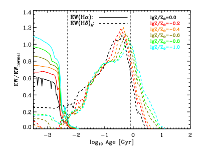
Figure 1.— Left panel: The scaled equivalent width of H$\alpha$ emission (solid lines) and H$\delta$ absorption (dashed lines) lines as a function of the age of single stellar populations for six different metallicities. The EW(H$\alpha$) is scaled to 10000 Å, and the EW(H$\delta$_A) is scaled to 10 Å. The two vertical dotted lines represent the fiducial ages of 5 Myr and 800 Myr, defining the windows of age traced by the H$\alpha$ emission and H$\delta$ absorption lines. Right panel: The 4000 Å break as a function of the age of single stellar populations for the different metallicities.

The three diagnostic parameters have long been used to indicate the recent SFHs on different timescales (e.g. Worthey & Ottaviani, 1997; Balogh et al., 1999; Kauffmann et al., 2003; Li et al., 2015; Wang et al., 2017, 2018). In SF galaxies, the H$\alpha$ emission mainly comes from the recombination of gas ionized by photons from extremely massive stars ($>$15${\rm M}_{\odot}$), which is therefore expected to trace the SFHs within the lifetime of these massive stars ($\sim$5 Myr). However, the EW(H$\delta$_A) traces the recent star formation within a longer timescale of more like 1 Gyr. The Balmer absorption lines arise from intermediate mass main-sequence stars with lifetimes of $\sim$1 Gyr. They are relatively insensitive to the metal abundance because they depend mostly on the behavior of the main-sequence turn-off temperature rather than the behavior of the red giant branch temperature (Worthey et al., 1994; Worthey & Ottaviani, 1997). Finally, the 4000 Å break is determined by the SFHs on still longer timescales with respect to EW(H$\delta$_A), and is found to be sensitive to the light-weighted stellar age (Balogh et al., 1999).

The evolution of these three diagnostic parameters for single stellar population (SSP) models of different metallicities can be seen by using the Flexible Stellar Population Synthesis code (FSPS; Conroy et al., 2009). FSPS is a powerful code that can generate spectra and absolute magnitudes of arbitrary stellar populations, with a series of flexible settings, such as metallicity, choice of stellar library, different IMF, and different evolutionary isochrones. Throughout this work, we will adopt the MILES stellar library (Sánchez-Blázquez et al., 2006; Falcón-Barroso et al., 2011), a Chabrier (2003) IMF, and the Padova isochrones (e.g. Bertelli et al., 1994, 2008), unless specified otherwise.

Nebular emission is produced by using the FSPS implementation of the photoionization code, CLOUDY (Byler et al., 2017). By simulating physical conditions within a gas cloud, CLOUDY predicts the thermal, ionization, and chemical structure of the cloud, and further produces the resultant spectrum of the diffuse emission (Ferland et al., 2013). In FSPS model, the ionizing radiation is produced by a point source at the central of a spherical shell of cloud, with assuming a constant gas density of $n_{\rm H}=100{\rm cm}^{-3}$. The fraction of the ionizing luminosity to escape from the HII region is assumed to be zero (Byler et al., 2017).

For each of our mock SFH, we produce the current-epoch spectrum for six metallicities ($\log_{10}Z/Z_{\odot}=$0.0, $-$0.2, $-$0.4, $-$0.6, $-$0.8 and $-$1.0), without implementing any dust attenuation. This means that the diagnostic parameters in the calibration are assumed to be dust-free. Being equivalent widths, the observed diagnostic parameters should, ideally, be independent of dust attenuation, but this will only be true if the nebular emission and stellar continuum have the same attenuation, which is unlikely to be the case. There are likely be second-order effects if different stellar populations have different dust obscuration. The correction of the observed diagnostic parameters for these second order dust effects will be presented in Section 2.6. Although we will only calibrate the SFR79 for the six discrete metallicities, we can obtain the SFR79 calibration for galaxies of other metallicities by linear interpolation in $\log_{10}Z/Z_{\odot}$ (see details in Section 3.1).

Figure 1 shows the evolution of EW(H$\alpha$), EW(H$\delta$_A) and D_n(4000) as a function of stellar age for SSP models at the six different metallicities. We present the evolution of EW(H$\alpha$) (solid lines) and EW(H$\delta$_A) (dashed lines) on the left panel of Figure 1. For all the different metallicities, the EW(H$\alpha$) is scaled to 10000 Å, and the EW(H$\delta$_A) is scaled to 10 Å. The two vertical dotted lines represent the ages of 5 Myr and 800 Myr respectively. As expected, after a single burst of star formation, EW(H$\alpha$) is large at first, but then quickly decays and becomes only 10% of its maximum value after 5 Myr, for all the six different metallicities. In addition, EW(H$\alpha$) is higher at lower metallicities. The dependence of EW(H$\alpha$) on metallicity comes from the nearly equal contribution of the variation in stellar continuum and the variation in H$\alpha$ emission.

For an SSP model with given metallicity, EW(H$\delta$_A) instead shows a peak at an age of a few hundred Myrs. The stellar population age corresponding to the peak EW(H$\delta$_A) decreases with metallicity. Rather than having a different timescale for each metallicity, we choose instead a standard timescale of 800 Myr for all metallicities that enables the defined change parameter SFR79 to be reasonably well calibrated at all the six metallicities. This however makes the SFR79 calibration dependent on metallicity. The D_n(4000) increases with increasing stellar age at a given metallicity, and increases with increasing metallicity at given stellar age.

Our definition of SFR79 is based on the SFR across two orders of magnitude in timescale, which is much larger than that of the widely-used “burstiness” based on H$\alpha$-to-UV ratio.

Further, as already noted the diagnostic parameters based on equivalent widths are insensitive to the dust attenuation and can be readily measured from the existing large body of optical spectra of galaxies, and are not strongly model-dependent. These conditions make the three diagnostic parameters to be an ideal choice to study the variability of SFR in galaxies.

2.3. Construction of the mock SFHs

Figure 2.— Illustrating the range of variation in the SFHs that are used in the calibration of SFR79. Each column of panels has the same $\tau_{\rm break}$, from left to right: 100 Myr, 500 Myr and 1000 Myr. Each row of panels has the same $\alpha$, from top to bottom: 1.0, 2.0 and 3.0.

In parametric SED modelling, strong priors are usually imposed on the SFHs. One of the widely used ones is the exponentially declining SFH (e.g. Bruzual A., 1983; Papovich et al., 2001; Shapley et al., 2005; Pozzetti et al., 2010; Carnall et al., 2019), i.e. the SFR is assumed to decline exponentially with some e-fold timescale $\tau$: ${\rm SFH}(t)\propto\exp(-t/\tau)$. However, it is clear in the real Universe, that the SFH of galaxies may be much more complicated than any assumed analytic formula. Motivated by the fact that the global SFD is well fit by a log-normal in time, Gladders et al. (2013) proposed that the log-normal form might also characterize the SFHs of individual galaxies (Dressler et al., 2013; Oemler et al., 2013; Abramson et al., 2015). Using the Illustris simulation, Diemer et al. (2017) investigated the SFHs for individual galaxies, and found that the log-normal form fits the overall shape of the majority of SFHs very well: 85% of cumulative SFHs are fitted to within a maximum error of 5% of the total stellar mass formed. The log-normal works systematically better than the commonly used exponentially declining model, and appears to be a reasonably good description for the global shape of SFHs for individual galaxies. Therefore we adopt the log-normal fits of the SFHs for Illustris galaxies (Diemer et al., 2017) as being representative of the global shape for the long-term variation of SFHs in the real Universe.

On top of these smoothly varying underlying SFH must be added short-term stochastic variations. We describe the stochastic variations in SFR in the frequency (or time) domain using the power spectrum distribution (PSD) of variations in the SFR. To construct the mock SFH, we use, for simplicity and following the work of Caplar & Tacchella (2019), a broken power-law PSD to characterize the possible variations in SFR that are superposed on the broad underlying log-normal SFH. The PSD can be written as:

$${\rm PSD}(\nu)=\frac{\sigma^{2}}{1+(\tau_{\rm break}\nu)^{\alpha}},$$ (1)

where $\nu$ is the frequency, $\sigma$ defines the amplitude of the PSD, $\alpha$ is the slope of PSD at the high frequency end, and $\tau_{\rm break}$ defines the break point where the PSD becomes flat towards lower frequency. We refer the reader to Caplar & Tacchella (2019) for more details of the properties of this kind of PSDs.

We then use a public IDL code to generate the random time series of variation in SFR with a given power spectrum distribution. Note that the variations of SFR are generated in logarithmic space. Figure 2 shows examples of the variations of stochastic components with different $\alpha$ and $\tau_{\rm break}$. Here we only show the variations with a time range of 2 Gyr, while in practise we generate the variation in time series over the full lifetime of the Universe. Following the work of Caplar & Tacchella (2019), the 1$\sigma$ scatter of the variations are normalized to 0.4 dex, which is comparable to the maximum scatter of SFMS in the observations (e.g. Whitaker et al., 2012; Speagle et al., 2014; Schreiber et al., 2015; Davies et al., 2019). The time resolution is set to be 1 Myr, which is much smaller than the SFH timescale traced by H$\alpha$, and smaller than the free-fall timescale of molecular clouds (Murray et al., 2010; Hollyhead et al., 2015; Freeman et al., 2017). As shown in Figure 2, larger $\alpha$ and longer $\tau_{\rm break}$ result in slower oscillations and stronger correlation in time domain.

In total, there are 29,203 galaxies in the Illustris simulation with stellar mass greater than $10^{9}$${\rm M}_{\odot}$ (Diemer et al., 2017). We do not yet exclude the quenched galaxies, but will do so later in Section 2.4 based on the EW(H$\alpha$) and EW(H$\delta$_A) of the mock spectra. For each of these 29,203 galaxies, with a given underlying log-normal SFH, we then construct 100 stochastic variations of the SFH by varying both $\alpha$ and $\tau_{\rm break}$ in logarithmic space, $\Delta_{\rm SFH}$ (see examples in Figure 2). The mock SFHs are then constructed by multiplying the log-normal SFH from Illustris galaxies with a factor 10${}^{\Delta_{\rm SFH}}$. We therefore have 2,920,300 mock SFHs in total. In practise, we make a 10$\times$10 grid for $\alpha$ and $\tau_{\rm break}$, where the two parameters are evenly spaced with $\alpha$ in the range of 1 to 3, and $\tau_{\rm break}$ in the range of 100 Myr to 1000 Myr. The ranges of the two parameters are chosen according to the result of Caplar & Tacchella (2019). Further, we find that the constrained slope of PSD is within this range in the second paper of this series. For each point on this grid, we generate a stochastic variation of SFH based on its $\alpha$ and $\tau_{\rm break}$ according to the approach above. We stress that our propose is not to try to model or reproduce the stochastic variation in SFHs in the real Universe, but is instead to simply generate a huge range of SFHs, which should cover the range of SFR79 that will be encountered in normal galaxies in the real Universe.

2.4. Calibration of SFR79

For each of the 2.9 million mock SFHs constructed above, we calculate the change parameter SFR79 at the present epoch, i.e. the simple ratio of the SFR averaged over the last 5 Myr to that averaged over the last 800Myr. Using the mock SFH and the SSP models, we can obtain the mock spectrum of the composite stellar population produced by each mock SFH by convolving the time varying spectrum of the SSP (at a given metallicity) with the detailed age distribution of each mock SFH. We can further compute the three diagnostic spectral parameters for each mock spectrum at the present epoch, for each of the six metallicities.

In practise, we do not of course need to produce an entire high resolution composite spectrum but simply measure the relevant input fluxes (or flux deficits) of the SSP once as a function of age from its evolving spectrum and then produce the diagnostic parameters for each mock SFH at the present epoch through a straight convolution of these functions with the age distribution of the SFH in question. For instance, the D_n(4000) is defined as the ratio of the flux density between the 4000 and 4100 Å ($f_{\rm red}$) and that between 3850 and 3950 Å ($f_{\rm blue}$) (Balogh et al., 1999). We first compute the evolution of $f_{\rm red}(t)$ and $f_{\rm blue}(t)$ with time for a SSP at a given metallicity. Then the $f_{\rm red}$ (or $f_{\rm blue}$) for a given mock SFH is the convolution of the corresponding age distribution $n(t)$ with the $f_{\rm red}(t)$ (or $f_{\rm blue}(t)$) evolution curve. In the similar way, the EW(H$\alpha$) and EW(H$\delta$_A) can also easily be obtained. The bandpasses for calculating D_n(4000) and EW(H$\delta$_A) are defined in Balogh et al. (1999). Specifically, the blue and red bandpass of wavelength (in Å) in calculating the D_n(4000) are [3850,3950] and [4000,4100]. The three bandpasses for the index of H$\delta$ absorption are [4083.50, 4122.25], [4041.60, 4079.75], and [4128.50, 4161.00]. In calculating emission (or absorption) line flux of H$\alpha$ (or H$\delta$), the contamination of the absorption (or emission) in H$\alpha$ (or H$\delta$) is corrected. We note that the approach in calculating the three diagnostic parameters for the mock spectra is exactly the same as that used in analysis of the observations in Section 3.1 (also see Wang et al., 2018).

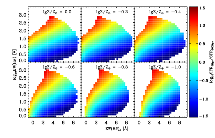
Figure 3.— The calibration of the SFR79 estimator in terms of EW(H$\alpha$) and EW(H$\delta$_A). The panels show the mean SFR79 as a function of the observed $\log_{10}$EW(H$\alpha$) vs. EW(H$\delta$_A) for the six different metallicities. Any effects of any differential reddening are not included in this calibration. Each panel represents the outcome of 2.9 million mock SFHs, as described in the text. The actual calibration used in this paper (Equation 2 and Table 1) includes also the D_n(4000).

2.4.1 SFR79 as a function of $EW(H\alpha)$ and $EW(H\delta_{A})$

Table 1The fitting parameters of the calibrator at different metallicities in Figure 4

$\log Z/Z_{\odot}$	a1	a2	a3	b1	b2	b3	c1	d	scatter	EW(H$\alpha$)	EW(H$\delta$A)
0.0	1.082	$-$0.06909	$-$0.01134	$-$0.2922	0.01167	$-$5.999e-05	$-$1.268	1.126	0.063	$>$1.0Å	$>-$1.0Å
$-$0.2	1.014	0.006220	$-$0.03168	$-$0.2958	0.01855	$-$7.570e-04	$-$0.8483	0.5110	0.065	$>$1.0Å	$>-$1.0Å
$-$0.4	1.006	0.04190	$-$0.03518	$-$0.2576	0.01338	$-$5.561e-04	$-$0.3489	$-$0.3272	0.062	$>$1.0Å	$>$0.0Å
$-$0.6	0.9310	0.1042	$-$0.04182	$-$0.3572	0.03650	$-$0.002370	0.1615	$-$0.8405	0.071	$>$1.0Å	$>$0.5Å
$-$0.8	0.9319	0.1067	$-$0.03414	$-$0.4048	0.04930	$-$0.003331	0.7171	$-$1.543	0.080	$>$1.0Å	$>$1.0Å
$-$1.0	0.8920	0.1293	$-$0.03305	$-$0.4694	0.06127	$-$0.004017	1.244	$-$2.091	0.090	$>$1.0Å	$>$1.5Å

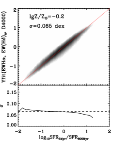
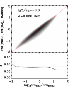
Figure 4.— Comparison of the SFR79 that is derived from the combination of $\log_{10}$EW(H$\alpha$), EW(H$\delta$_A), and D_n(4000) with the actual SFR79 as directly calculated from the SFH for the 2.9 million mock galaxies, for six different metallicities. The lower panels in each figure, show the dispersion between the fitted SFR79 and the real SFR79 as a function of the real SFR79. This is largely independent of SFR79, but increases somewhat to lower metallicities because of the variation of EW(H$\delta$_A)(t) shown in Figure 1.

Now that we have the measurements of SFR79 as well as the diagnostic parameters for millions of mock SFHs, it is straightforward to search for the solution of SFR79 as a function of the three diagnostic parameters. Figure 3 shows the $\log_{10}$EW(H$\alpha$) vs. EW(H$\delta$_A) diagram with the color-coding of SFR79 for the six different metallicities. The SFR79 shows clear gradients on this diagram, confirming that the EW(H$\delta$_A) and $\log_{10}$EW(H$\alpha$) indeed contain information on the change parameter. For all metallicities, at fixed EW(H$\delta$_A), the SFR79 increases with increasing $\log_{10}$EW(H$\alpha$); at fixed $\log_{10}$EW(H$\alpha$), the SFR79 decreases with increasing EW(H$\delta$_A). This is as expected, since the two parameters indicate the strength of star formation at two different timescales. Another interesting feature is that the range of EW(H$\delta$_A) becomes smaller towards smaller metallicity. This is due to the different evolution curves of EW(H$\delta$_A) for the SSP models at the different metallicities (see Figure 1). For the lowest metallicity ($\log_{10}Z/Z_{\odot}=-1.0$), the EW(H$\delta$_A) of the SSP is greater than zero over the entire age range of 10 Gyr after a single starburst. This is the reason why there is no data points with EW(H$\delta$_A) below zero at the lowest metallicity. Note that EW(H$\delta$_A) is here defined to be positive for absorption.

After exploring many kinds of combination of the three parameters, we find that a combination of polynomials to the third-order can well reproduce the values of SFR79  to within a scatter of 0.06-0.09 dex. The form of the polynomials can be written as:

$$\begin{split}\log_{10}{\rm SFR79}=&a1\times x+a2\times x^{2}+a3\times x^{3}\\ &+b1\times y+b2\times y^{2}+b3\times y^{3}\\ &+c1\times z+d,\\ \end{split}$$ (2)

where $x=$ $\log_{10}$EW(H$\alpha$), $y=$ EW(H$\delta$_A), $z=$ D_n(4000), and $a1$, $a2$, $a3$, $b1$, $b2$, $b3$, $c1$ and $d$ are parameters determined from the fittings. The fitting parameters for different metallicities are listed in Table 1. During the fittings, we exclude mock spectra with extremely low EW(H$\alpha$) and EW(H$\delta$_A), since these are not encountered in the star-forming galaxies that are of interest in this work. The exclusion thresholds of these two parameters at different metallicities are listed in the last two column of Table 1. As shown in Table 1, the threshold of EW(H$\alpha$) is 1Å for all metallicities, while the threshold of EW(H$\delta$_A) increases with decreasing metallicity, varying from $-$1Å to 1.5Å. The exclusion of quenched galaxies with very small EW(H$\alpha$) and EW(H$\delta$_A) is immaterial for the present purposes. We also note that very small values of these two parameters would anyway be associated with relatively large observational uncertainties.

Figure 4 compares the SFR79 as directly measured from the mock SFHs with the results obtained from Equation 2 using the three diagnostic parameters. As shown, even though we included a huge range of possibilities in the mock SFH construction, the SFR79 can be very well determined by the combination of these three diagnostic parameters with a scatter of 0.06-0.09 dex. The scatter shows very little dependence on SFR79 for almost all the metallicities examined. Another interesting feature is that the scatter becomes larger with decreasing metallicity. This is due to the fact that we use a fixed timescale of 800 Myr to define the change parameter for all the metallicities. In principle, we could have increased the averaging timescale to $\sim$1 Gyr to reduce the scatter in the calibrator at low metallicities. However, this variable timescale would introduce more complexity in analyzing the results in Section 4 and 5. We therefore decided to keep the timescale constant for the different metallicities. The chosen timescale of 800 Myr was selected to minimize the scatter of calibrators at the three highest metallicities ($\log_{10}Z/Z_{\odot}=$0.0, $-$0.2, and $-$0.4), in which most of our sample galaxies are in fact located (see Section 2.4.2).

2.4.2 The performance of the calibrator

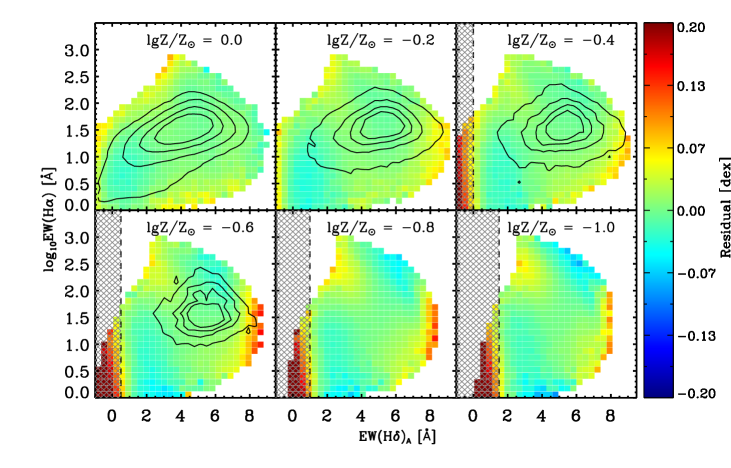
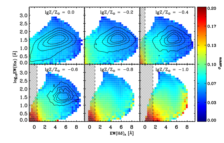
Figure 5.— The mean offset (upper panels) and dispersion (lower panels) in the recovered SFR79 compared with the true SFR79 across the $\log_{10}$EW(H$\alpha$) vs. EW(H$\delta$_A) diagram for the mock galaxies at the six metallicities. The recovered SFR79 is calculated based on Equation 2. This means that the D_n(4000) is also included in calculating SFR79, although here we only present the dependence of EW(H$\alpha$) and EW(H$\delta$_A). The shaded regions are considered to be beyond the valid regions of the calibrator (see also Table 1). In each panel, the black contours show the distribution of the spaxels from the MaNGA SF galaxies of the corresponding metallicity. The observed EW(H$\alpha$) and EW(H$\delta$_A) of MaNGA spaxels are corrected for the dust attenuation according to the approach described in Section 2.6. The black contours enclose 30%, 50%, 70% and 90% of spaxels from the inside outwards.

We showed in the above subsection that SFR79 could be calibrated with an overall uncertainty of 0.06-0.09 dex. In this subsection, we examine the performance of the calibrator in the $\log_{10}$EW(H$\alpha$) vs. EW(H$\delta$_A) diagram, to examine the performance of the SFR79 estimator in different regions of the diagram.

We show the $\log_{10}$EW(H$\alpha$) vs. EW(H$\delta$_A) diagram for the mock SFHs with the color-coding of the $\Delta$SFR79 in the top group of panels in Figure 5. The $\Delta$SFR79 is defined as the difference between the SFR79 from Equation 2 and the true SFR79 in the mock SFHs. At each metallicity, we also present the distribution of the spaxels from the MaNGA SF galaxies (of the corresponding metallicity, with bins of width of 0.2 dex) on the $\log_{10}$EW(H$\alpha$) vs. EW(H$\delta$_A) diagram, shown in black contours. The stellar metallicity of the sample galaxies is taken from the empirical mass-metallicity relation from Zahid et al. (2017) (see Equation 4 in Section 3.1). Most of the sample galaxies are in the three highest metallicity bins, and there are no contours in the two lowest metallicity bins. This is because the number of spaxels in the two lowest metallicity bins are quite limited (only one galaxy in the sample has a metallicity in each of these two lowest bins).

As shown, the calibration formula can indeed give an excellent estimation of SFR79. However, we note that the estimator does not work well when EW(H$\delta$_A) and EW(H$\alpha$) lie beyond the threshold criteria of the calibrator (see the shaded regions of Figure 5 and also Table 1). In addition, although our mock SFHs cover a very wide range on the diagram of $\log_{10}$EW(H$\alpha$) vs. EW(H$\delta$_A), some regions of parameter space are still not covered (the white regions in Figure 5). The calibration polynomial is clearly not valid for the data points that are beyond the colored regions. This limitation does not affect our application to MaNGA galaxies, because almost all the spaxels of the SF galaxies in MaNGA are within the regions of validity for the estimator (see the black contours).

At the three lowest metallicities, the estimator appears to systematically underestimate the SFR79 by up to $\sim$0.1 dex at the high EW(H$\delta$_A) end (see yellow and red colors at high EW(H$\delta$_A) in Figure 5). This may be due to the fact that at the edge of the parameter space, the number density of mock SFH is relative low, which contribute a small weight during the fitting. However, this systematic deviation in the calibrator is not a problem, since it can be easily corrected based on the position of the $\log_{10}$EW(H$\alpha$)-EW(H$\delta$_A) diagram in the application. We perform this correction in applying the calibrator to MaNGA galaxies. We note that this correction is very minor, since in the observation almost all the data points from MaNGA located in the regions that the calibrator operates rather well.

In principle, we could of course simply establish a look-up table for SFR79 over the whole range of the three diagnostic parameters, so as to avoid the above correction. However, in this work, we prefer to present a simple empirical formula of SFR79 which can be used by readers.

We show the scatter in $\Delta$SFR79 on the $\log_{10}$EW(H$\alpha$) vs. EW(H$\delta$_A) diagram in the bottom group of panels in Figure 5. As a whole, for all the metallicities explored, the scatter of the calibrator is small at the high end of both $\log_{10}$EW(H$\alpha$) and EW(H$\delta$_A), and increases towards the lower end of $\log_{10}$EW(H$\alpha$) and EW(H$\delta$_A). This may be due to the fact that for high $\log_{10}$EW(H$\alpha$) and EW(H$\delta$_A) (corresponding to high recent SFRs), the contribution from the older stellar populations in the measurement of these two parameters is correspondingly small. With increasing metallicity, the scatter decreases as a whole, which is likely due to the timescale of 800 Myr in definition of the change parameter for all the metallicities discussed above.

Based on the bottom panels of Figure 5, we assign an uncertainty in the SFR79 according to the location on the $\log_{10}$EW(H$\alpha$) vs. EW(H$\delta$_A) diagram in the application of the calibrator. While the scatter of SFR79 in the mock SFHs may over-estimate the uncertainty of SFR79 for an individual galaxy because the mock SFHs may contain not found ones in the real Universe, we think that this is a more reasonable approach than simply assigning a constant uncertainty of SFR79 at a given metallicity based on Figure 4. Since this uncertainty is due to the estimator itself, we refer to this uncertainty as “model uncertainty”. This is distinct from the uncertainty due to measurement uncertainties of the three diagnostic parameters from the observations (see Section 4.1).

2.5. The effect of changing the IMF and the evolutionary isochrones

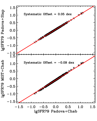
Figure 6.— The impact of changing the IMF and evolutionary isochrones on the calibration of SFR79 for MaNGA galaxies with stellar mass greater than $10^{10}$${\rm M}_{\odot}$. Upper panel: the SFR79 calibrated for Padova isochrones and the Chabrier IMF versus the SFR79 calibrated with same isochrones and the Salpeter IMF. Lower panels: the SFR79 calibrated with the Padova isochrones and the Chabrier IMF versus the SFR79 calibrated with MIST isochrones and the same IMF. In the upper panel, the red line is parallel to but 0.05 dex above the one-to-one line, while in the lower panel, the red line is parallel to but 0.09 dex below the one-to-one line, indicating that the effects of these two changes is to introduce a uniform offset in SFR79.

In deriving the calibration for SFR79  we assumed for each mock galaxy the same, non-evolving, IMF of Chabrier (2003). This assumption may not be the case in the real Universe. In principle, a time-varying IMF and a time-varying SFH are deeply degenerate, since we have no way of knowing when stars below the stellar Main Sequence turn-off stars produced. We do not consider this issue further in the current work, but this should not be a problem unless the cosmic evolution of the IMF was significant in the last $\sim$1 Gyr (the timescale used in definition of the change parameter), which we consider unlikely.

However, the IMF may also be different from galaxy to galaxy, or even in different parts of the same galaxy. Based on a very sensitive index of the IMF, ¹³CO/C¹⁸O, Zhang et al. (2018) found evidence of a top-heavy stellar IMF (with respect to Chabrier IMF) in the dusty starburst galaxies at redshift $\sim$2-3.

In this subsection, we examine the stability of our calibrator with different IMFs, choosing to do this, for simplicity, only at a single (solar) metallicity. Based on the same approach in Section 2.3 and 2.4, we construct a new calibration of SFR79 using a Salpeter IMF (Salpeter, 1955) without changing the other settings. Then we compare the two calibrators by applying them to a sample of MaNGA galaxies with stellar mass greater than $10^{10}$${\rm M}_{\odot}$. The three diagnostic parameters of MaNGA galaxies are calculated based on the spectra binned within the effective radius. Details of the binning scheme are in Section 3.4. Note that the three diagnostic parameters are corrected for the dust attenuation, according to the approach in Section 2.6. As shown in the top panel of Figure 6, the change of IMF gives the same result but with a systematic offset of about 0.05 dex. It is to be expected that a change in the IMF produces a systematic offset in SFR79 because both IMF and SFR79 will change the relative number of stars of different masses.

In our work, the absolute value of SFR79 is of less interest than the dispersion in SFR79. Therefore we argue that the choice of IMF is, at least within the range of plausible possibilities, not important.

We next examine the stability of the SFR79 calibration with respect to the use of different stellar evolution model, i.e. the isochrones. In the similar way, we generate a new calibrator by adopting the MIST isochrone (e.g. Paxton et al., 2011; Choi et al., 2016; Dotter, 2016; Paxton et al., 2018) with all other settings unchanged. The result is shown in the bottom panel of Figure 6. Again we see that the use of MIST isochrones introduces a small systematic offset of $-$0.09 dex.

While these effects introduce systematic offsets to SFR79, this will not affect the investigation of the temporal variation of SFR in galaxy populations, because it is the scatter of SFR79 that characterizes this variation, rather than the average value (Broussard et al., 2019). A significant problem would occur only if the IMF or the appropriate isochrones varied significantly from galaxy to galaxy. While the former is possible, the latter is presumably not. We note at this point that the variation with IMF (systematic offsets of 0.05 dex) is rather small compared with the observed dispersion in SFR79 within the population, which is 0.23 dex (see Section 4 below). So, we can assume that any variations in IMF are probably a negligible contributor to this scatter.

2.6. Correction for dust attenuation

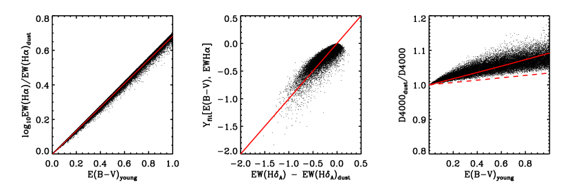
Figure 7.— Correction of the observed values of $\log_{10}$EW(H$\alpha$), EW(H$\delta$_A) and D_n(4000) for dust attenuation as required before application of the calibrator to the observational data. Left-hand panel: the change in $\log_{10}{\rm EW}({\rm H}\alpha)$ as a function of E(B$-$V)_young. Middle panel: the correction of EW(H$\delta$_A) with E(B$-$V)_young and EW(H$\alpha$). Right-hand panel: the change in D_n(4000)${}_{\rm dust}/$D_n(4000) as a function of E(B$-$V)_young. The red lines are the fitting result of the corrections (see Equation 3). In the right-hand panel, the red dashed line is the analytical relation computed with assuming that the value of E(B$-$V) does not change with time. Here we only present the correction at solar metallicity for illustration.

Table 2The fitting parameters of the dust attenuation for three diagnostic parameters in Figure 7

$\log_{\rm 10}Z/Z_{\odot}$	p1	p2	p3	p4	p5	$\log_{10}$EW(H$\alpha$)ERR	EW(H$\delta$A)ERR	Dn(4000)ERR
0.0	0.685	$-$0.00582	0.580	$-$4.29	0.0382	0.01 dex	0.098 Å	0.019
$-$0.2	0.687	$-$0.00691	0.569	8.23	0.0345	0.01 dex	0.084 Å	0.016
$-$0.4	0.689	$-$0.00595	0.576	12.5	0.0318	0.009 dex	0.072 Å	0.014
$-$0.6	0.691	$-$0.00496	0.564	14.4	0.0306	0.008 dex	0.063 Å	0.014
$-$0.8	0.693	$-$0.00407	0.565	15.1	0.0287	0.007 dex	0.052 Å	0.012
$-$1.0	0.692	$-$0.00388	0.563	16.4	0.0275	0.007 dex	0.050 Å	0.011

As described above, we did not include the effects of dust attenuation in the calibration of SFR79. This means that any correction for dust attenuation correction must be made to the three observational parameters before feeding them into the SFR79 calibration. As already noted, the use of equivalent widths makes them relatively insensitive to extinction. However, differential extinction between stars of different ages, or between line and continuum emission is more of a problem. Newly formed stars ($<10$ Myr) may have different extinction than older stars, since the extinctions of stellar continuum and of nebular emission are usually different (e.g. Calzetti et al., 2000; Moustakas & Kennicutt, 2006; Wild et al., 2011; Hemmati et al., 2015). Charlot & Fall (2000) proposed a two-component dust model, where the optical depth for stellar populations older than 10 Myr is around one-third of the optical depth of stellar populations younger than 10 Myr. In this model, the regions of young stellar populations are more dusty than the regions of older stellar populations, because the newly formed stars are embedded in molecular clouds. The demarcation timescale of 10 Myr comes from the timescale of disruption of molecular clouds (Blitz & Shu, 1980; Murray et al., 2010; Conroy et al., 2009). In this work, we make the same assumption of this stellar age dependent dust model, and we adopt the Cardelli-Clayton-Mathis (CCM) dust attenuation curve (Cardelli et al., 1989).

With this dust model, we correct the dust attenuation of the three diagnostic parameters in the following way. First, we generate as before mock SFHs based on the SFHs of Illustris galaxies adding stochastic processes, but here adopt a broken power-law PSD of SFHs with $\alpha=$1.5 and $\tau_{\rm break}=$20 Gyr (The large $\tau_{\rm break}$ make the PSD close to a single power-law PSD with $\alpha$=1.5). And again, the scatter of the variations are normalized to 0.4 dex. In contrast to the situation in Section 2.3, we here try to generate SFHs that resemble the observations, rather than a huge range of all possibible SFH. A power-law PSD with $\alpha=$1.5 is likely a good description of the stochasticity of SFHs without considering the intrinsic scatter of the SFMS, according to the analysis of our second paper of this series. Actually, in the second paper, we will find that, if we assume a single power-law form for the PSD of the specific SFH, a slope of 1.5 is the best to reproduce the distribution of galaxies on the $\Delta$sSFR7-$\Delta$sSFR9 plane . The slope of PSD adopted here is slightly shallower than the one assumed in Caplar & Tacchella (2019), who assumed a PSD index of 2, corresponding to a random walk process. We refer the reader to the second paper of this series for details.

We then calculate two sets of diagnostic observational parameters based on the mock SFHs with and without the dust attenuation. For the mock spectra, we know the contribution of the stellar populations at different ages, from the mock SFHs and evolving spectra of the SSP models. This enables us to apply a stellar-age-dependent extinction model to obtain the reddened spectra and the values of the three diagnostic parameters. The diagnostic parameters with dust reddening are denoted as D_n(4000)_dust, EW(H$\delta$_A)_dust and EW(H$\delta$_A)_dust. In this process, we assign for each galaxy an E(B$-$V)_young, i.e. the E(B$-$V) for the stellar population younger than 10 Myr, that is randomly distributed between 0.0 and 1.0. At last, we compare the two set of observed parameters and define recipes for the correction.

After exploring many forms for the dust correction of the three observational parameters, we found good expressions with rather small uncertainties. Figure 7 presents the formulae to correct the dust attenuation (solid red lines) by comparing the two set of diagnostic parameters at solar metallicity. The correction of EW(H$\alpha$) and D_n(4000) are a function of E(B$-$V)_young, while the correction of EW(H$\delta$_A) is a function of both E(B$-$V)_young and EW(H$\alpha$). In the observation, the E(B$-$V)_young can be determined from the flux ratio of H$\alpha$ and H$\beta$ using the Balmer decrement. The adopted expressions for the correction for the three parameters are as follows:

$$\begin{split}\log_{10}{\rm EW}({\rm H}_{\alpha})/{\rm EW}({\rm H}_{\alpha})_{\rm dust}=&p1\times{\rm E(B-V)}_{\rm young}\\ {\rm EW}({\rm H}\delta_{\rm A})-{\rm EW}({\rm H}\delta_{\rm A})_{\rm dust}=&p2\times{\rm E(B-V)}_{\rm young}^{p3}\\ &\times({\rm EW}({\rm H}_{\alpha})+p4)\\ \log_{10}D_{n}(4000)_{\rm dust}/D_{n}(4000)=&p5\times{\rm E(B-V)}_{\rm young},\end{split}$$ (3)

where $p1$, $p2$, $p3$, $p4$, and $p5$ are parameters determined by fitting. Table 2 shows these fitting parameters to be used in Equation 3, as well as the resulting uncertainties of the observational diagnostic parameters (listed in the last three columns in Table 2) produced by the dust attenuation correction, at different metallicities. The uncertainties are determined by the scatters in the three panels of Figure 7. As can be seen in Table 2, the uncertainties due to this correction are small.

However, there may be additional uncertainties in the dust attenuation correction, due to possible variations in the f-factor (e.g. Kashino et al., 2013; Lin & Kong, 2019; Faisst et al., 2019), defined as the E(B$-$V)_star/E(B$-$V)_nebular, from galaxy to galaxy or from regions to regions. This effect is not included in our dust model in the present work. Specifically, by using the MaNGA galaxies, Lin & Kong (2019) found that the f-factor decreases with increasing stellar mass, and slightly increases with increasing sSFR. For most of SF spaxels in galaxies above 10¹⁰${\rm M}_{\odot}$, the f-factor is in the range of 0.3-0.7 with a scatter of $\sim$0.1-0.15. We have examined the dependence of our SFR79 estimator on the value of E(B$-$V)_old/E(B$-$V)_young at solar metallicity. Increasing E(B$-$V)_old/E(B$-$V)_young by 0.1, the resulting SFR79 show an overall 0.03 dex offset with respect to the old ones, which is much smaller than the scatter of SFR79 (0.23 dex) we measured in Section 4. We conclude that the dust attenuation corrections of the three parameters are only a secondary effect due to the fact that they are relative values measured at fixed wavelength. The uncertainty of the dust attenuation is even much smaller than the value of the applied correction for the three parameters, and is therefore not likely to be a big concern.

3. Application to MaNGA galaxies

In this section of the paper, we apply the SFR79 estimator constructed in Section 2 to spatially-resolved spectroscopic data from the MaNGA survey. In Section 3.1, we will give a brief introduction for the sample selection and the measurements of the relevant parameters. In Section 3.2, we examine the consistency for the overall change in SFR. In Section 3.3, we then derive a small additional correction of SFR79 parameter to correct for an unexpected apparent dependence of SFR79 on stellar surface density.

3.1. The sample galaxies and the measurement of parameters

MaNGA is one of the largest integral field spectroscopic surveys, aiming at obtaining the two-dimensional spectra for $\sim$10,000 galaxies in the redshift range of $0.01<z<0.15$ (Bundy et al., 2015). The wavelength covered by MaNGA is 3600-10300 Å at a spectral resolution R $\sim$2000, which is sufficient to accurately measure the three diagnostic parameters (Li et al., 2015) used in this paper.

In this work, we utilize the well-defined sample of star-forming galaxy from W19. Here we therefore only briefly describe the sample definition, and refer the reader to W19 for further details.

The galaxy sample is originally selected from SDSS Data Release 14 (Abolfathi et al., 2018), excluding the mergers, irregulars, heavily disturbed galaxies, as well as galaxies for which the median S/N of the 5500 Å continuum is less than 3.0 at their effective radii. The quenched galaxies are excluded based on the stellar mass and SFR diagram. The stellar mass and SFR are measured within the effective radius, i.e. $M_{\ast}$($<$$R_{\rm e}$) and SFR($<$$R_{\rm e}$), based on the MaNGA spectra. Our final sample consists of 976 SF galaxies, and is a representative sample of SF main-sequence galaxies in the low-redshift Universe.

The stellar mass maps of MaNGA galaxies are derived from the public fitting code STARLIGHT (Cid Fernandes et al., 2004), using SSPs with Padova isochrones from Bruzual & Charlot (2003) and the Chabrier (2003) IMF. The SFR maps are determined by the extinction-corrected H$\alpha$ luminosity adopting the conversion formula to SFR from Kennicutt (1998), again using a Chabrier (2003) IMF. The uncertainty in determining the SFR via this approach is 15% (or $\sim$0.06 dex), due to the variations in the electron temperature in the range $T_{\rm e}=$5000-20000 K (Osterbrock & Ferland, 2006). As above, we also refer to this uncertainty as model uncertainty.

Since in this work our purpose is primarily to investigate the SFR of galaxies on different timescales, we denote the SFR directly determined from the H$\alpha$ luminosity as SFR7, i.e. SFR_5Myr (see Figure 1). The intrinsic extinction for nebular emission is measured based on the Balmer decrement, assuming the CCM dust attenuation curve (Cardelli et al., 1989) and Case B recombination with ab intrinsic flux ratio of H${\alpha}$/H$\beta$ = 2.86. The E(B$-$V) for nebular emission is then a good estimation for the E(B$-$V)_young, i.e. the color excess for the stellar population younger than 10 Myr. We note that the IMF, isochrones, and dust attenuation curve that are used to obtain the stellar masses and SFR_5Myr are consistent with those used in Section 2.

The strengths of the emission lines are measured based on the stellar continuum-subtracted spectrum by fitting a Gaussian profile to the lines. The D_n(4000) and EW(H$\delta$_A) are directly measured based on the observed spectra after subtracting emission lines, rather than from the best-fit continuum spectra. This avoids the uncertainties of the measurements due to the possible systematic offset (especially at 3800-4200 Å) between the model spectra and observed ones. For many SF galaxies, the bottom of the H$\delta$ absorption is usually accompanied by weak H$\delta$ emission, which make the EW(H$\delta$_A) difficult to measure. In this work, we take advantage of the $\chi^{2}$ minimization spectral fitting code developed by Li et al. (2005), which can effectively mask the emission-line regions iteratively during the fitting. This is critical to accurately model the absorption troughs and also characterize the emission lines (see examples in Li et al. (2015)).

Before applying our SFR79 estimator on the MaNGA galaxies, we first correct the three diagnostic parameters for dust attenuation based on Equation 3. Since both the estimator and the dust attenuation correction depend on the stellar metallicity of galaxies, we adopt the stellar mass-metallicity relation from Zahid et al. (2017) to estimate the stellar metallicity of individual galaxies. The relation can be written as:

$$\log_{10}\frac{Z}{Z_{\odot}}=Z_{0}+\log_{10}\left[1-\exp\left(-\left[\frac{M_{*}}{M_{0}}\right]^{\gamma}\right)\right],$$ (4)

where $Z_{0}$ = 0.075, $M_{0}$ = 10^9.79${\rm M}_{\odot}$, and $\gamma$ = 0.56. This relation is determined by modelling the galaxy spectra with a linear combination of sequential single burst model spectra. For a given set of three observational parameters at given metallicity, we first calculate the correction based on Equation 3 and Table 2 at the two closest metallicities. Then we use linear interpolation in $\log_{10}Z/Z_{\odot}$ to obtain the corrections of the observational three diagnostic parameters at the required metallicity. In the similar way, we then obtain the SFR79 using the (dust-corrected) values of the three diagnostic parameters by calculating the SFR79 at the two closest metallicities based on Equation 2 and Table 1 then obtain the SFR79 at the required metallicity via linear interpolation in $\log_{10}Z/Z_{\odot}$.

3.2. Consistency check: the overall change in SFR

Having calculated SFR79 for all spaxels in our MaNGA sample, we can now carry out an important consistency check by calculating the total SFR of all spaxels in the sample, averaged over the last 5 Myr, and the total SFR averaged over the last 800 Myr. These should be roughly equal. To be precise, the ratio of these, i.e. $\langle{\rm SFR7}\rangle/\langle{\rm SFR9}\rangle$, should reflect the overall cosmic evolution of the SFR of the SF galaxy population over the last Gyr, i.e. the change in overall SFR of SF galaxies that is implied by integrating the change in the sSFR of the Main Sequence. The cosmic evolution of $\log_{10}\langle{\rm SFR7}\rangle/\langle{\rm SFR9}\rangle$ that is expected for the ensemble of main-sequence galaxies is calculated to be $-$0.025 dex based on the evolution of the sSFR of the SFMS from Lilly & Carollo (2016), and the stellar mass function for SF galaxies from Peng et al. (2010).

The ratio of these two total SFR in the MaNGA data (using our estimator of SFR79 to calculate individual SFR9) is actually $-0.066$ dex, which is reassuringly close (within 0.04 dex, or 10%) to the expected value. This very satisfactory agreement should be taken as a first confirmation that our calibration of SFR79 is quite accurate and certainly usable. In fact, given the assumptions that we made, however reasonably, about the effect of reddening, about the form of the IMF and about the choice of stellar evolution isochrones, the very close agreement to within 0.04 dex should probably be seen as fortuitous. This is explored further in the next subsection.

3.3. Correction of a dependence of $\Sigma_{*}$

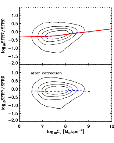
Figure 8.— Correction of the presumed spurious dependence of SFR79 on $\Sigma_{*}$. The blue dashed lines show the median SFR79 at given $\Sigma_{*}$. The upper panel shows the raw SFR79 (upper panel) as a function of $\Sigma_{*}$ for the spaxels selected from MaNGA galaxies. Since, as discussed in the text, the increase with $\Sigma_{*}$ is thought to be spurious, this median relation is used to correct the SFR79 using a simple broken power-law shown with the red line. The lower panel shows the distribution of SFR79 in the spaxels after this correction. In both panels, the contours show the number density distribution of the spaxels in the sample.

The top panel of Figure 8 shows the SFR79 for all the spaxels in our sample galaxies as a function of de-projected stellar mass surface density ($\Sigma_{*}$) . The contours show the overall number density distribution of spaxels in this diagram. These contours enclose 30%, 50%, 70% and 90% of all spaxels, from the inside out. The blue dashed line shows the median SFR79 at given $\Sigma_{*}$. Based on SFR79, we can obtain $\log_{10}$SFR9, i.e. $\log_{\rm 10}{\rm SFR}_{\rm 800Myr}$, for each individual spaxel of the sample galaxies.

It is clear in this figure that the mean SFR79 appears to slightly increase with increasing $\Sigma_{*}$, suggesting that SF galaxies have on average a slightly negative SFR79 radial gradient. We suspect that this small effect is unlikely to be real, since it would suggest that the SFR was declining more at large radii, leading to a negative gradient in the rate of change of the sSFR of galaxies. Since galaxies generally have a positive gradient in sSFR at the current epoch, this would imply that this gradient was weakening. If anything, we would expect the opposite trend in any “inside-out” scenario of galaxy evolution. There are other reasons to question this small gradient in SFR79. Not least, although the dust-correction is in principle computed locally, we did not consider any radial variation of the form of the dust-correction, nor of the stellar metallicity (e.g. Zheng et al., 2017; Goddard et al., 2017), nor any (possible) radial variation of IMF (Gunawardhana et al., 2011) in the estimation of SFR79. We suspect that some combination of these may be the cause of the trend in the upper panel of Figure 8.

Accordingly, we therefore perform a small ad hoc correction to the values of SFR79 as a function of $\Sigma_{*}$ (only). This is constructed so as to eliminate the dependence of SFR79 on $\Sigma_{*}$, while not significantly perturbing the total rates of star-formation, as discussed in the previous sub-section. We first fit the median SFR79-$\Sigma_{*}$ relation with a piecewise linear function, shown as the red line in Figure 8. The red line is in the form of

$$y=\begin{cases}0.04581x-0.6089,&x<7.5,\\ 0.1737x-1.568,&x\geq 7.5,\\ \end{cases}$$ (5)

where y = $\log_{10}$SFR79, and x=$\log_{10}\Sigma_{*}$ [$M_{\odot}{\rm kpc}^{-2}$]. For each spaxel, we then subtract this median SFR79 at the corresponding $\Sigma_{*}$. In order to preserve the total star-formation rates, as discussed in the previous sub-section, we then add a uniform $-0.136$ dex to the SFR79  computing this value to exactly match the $\log_{10}\langle{\rm SFR7}\rangle/\langle{\rm SFR9}\rangle$ with the value of the cosmic evolution for SF main-sequence galaxies (i.e. including the 0.04 dex offset discussed in the previous sub-section). The bottom panel of Figure 8 shows the SFR79 as a function of $\Sigma_{*}$ after this correction.

This correction to SFR79 is of course quite arbitrary. However, we stress that this correction only makes the overall SFR79 profile flat, and does not change the scatter of SFR79 at given $\Sigma_{*}$. Since the variability of SFHs is indicated by the scatter of SFR79 across the population, rather than by its average or median value, this correction will not significantly affect any of our conclusions in the following analysis. In the remainder of this work, the SFR79 for both individual spaxels and individual galaxies will be corrected according to the above approach.

3.4. The SFR79 maps and profiles

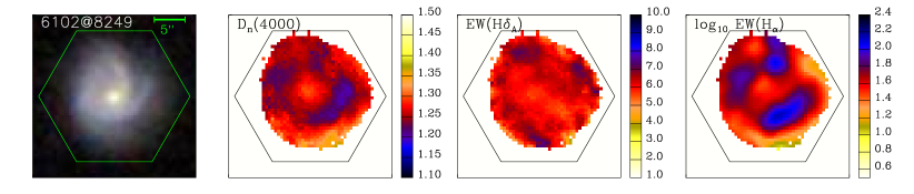
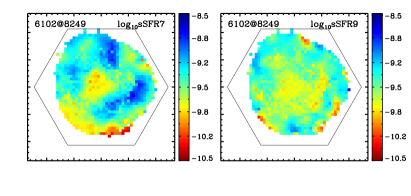
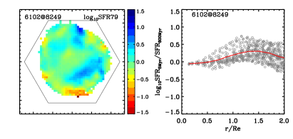
Figure 9.— An example of the measurements and derived quantities for the MaNGA galaxy 6102@8249. The top panels show from left to right, the SDSS color image, and maps of the 4000Å break, the H$\delta_{\rm A}$ index, and $\log_{10}{\rm EW}({\rm H}\alpha)$. The hexagons represent the area covered by the IFS bundles on this galaxy. The bottom panels show from left to right, the maps of $\log_{10}$sSFR7, of $\log_{10}$sSFR9, and of $\log_{10}$SFR79, together with the SFR79 profile of this galaxy. In the bottom rightmost panel, the gray circles represent the individual spaxels, and the red line show the SFR79 profile, which are calculated based on the binned diagnostic parameters within a set of annulus.

Based on the approach in Section 3, we can now obtain the SFR79 maps of each sample galaxy. Figure 9 shows an example of the measurements for one typical galaxy (MaNGA-ID: 8249-6102). The top panels of Figure 9 shows the SDSS color image, D_n(4000), EW(H$\delta$_A), and $\log_{10}$EW(H$\alpha$) maps from left to right, respectively. It should be noted that the three diagnostic parameters are shown prior to the correction for dust attenuation. The bottom panels show the maps of sSFR7, sSFR9, and SFR79, as well as the profile of SFR79 for this galaxy, from left to right, respectively.

As shown, the EW(H$\alpha$) map shows clumpy features (blue clumps), corresponding to the regions with high recent star formation within 5 Myr. However, these regions do not show high EW(H$\delta$_A), suggesting that the star formation in these regions were not unusually active in forming stars during the last $\sim$1 Gyr. Thus, the current star formation in these blue clumps of $\log_{10}$EW(H$\alpha$) map is triggered recently (much less than 800Myr). Consistent with this, these regions are seen as positive (blue) on the SFR79 map that blue clumps are seen in the same regions. On the other hand, some regions with high EW(H$\delta$_A) but relative low EW(H$\alpha$), are visible on the SFR79 map with yellow clumps. The star formation of these regions is reduced in a time scale much less than 800 Myr. This simple example indicates that the SFR79 we measured is indeed meaningful, and provide the quantitative description for the above effect.

In the bottom rightmost panel of Figure 9, the small gray circles indicate the SFR79 derived spaxel-by-spaxel in this galaxy, while the red line shows the SFR79 profile obtained from the binned spectra in annular bins. It can be clearly seen that, between 0.5-1.0$R_{\rm e}$  the distribution of SFR79 is asymmetric: most of the spaxels have a relative low SFR79, while a small fraction of spaxels have increased SFR79. This is due no doubt to the duty cycle of star formation. At any given time, star-formation in a given region of galaxy is found in a limited number of active regions, which themselves are active for only a short fraction of the time.

In the current work, we do not wish to study the variation of SFR (or SFR79) that is caused by this small scale local effect but rather focus on the variations in SFR on larger scales. Therefore we use a binning scheme to average out these small scale spatial effects.

The diagnostic parameters for a given radial bin are calculated in the following way. For instance, for D_n(4000), we first calculate the flux density of the blue and red bandpass near 4000 Å as described in Section 2.4 for all the spaxels (with S/Ns greater than 3 at 5500 Å) in a given radial bin. The D_n(4000) of this radial bin is then obtained from the ratio of the sum of the flux densities in the red bandpass to the sum of them in the blue bandpass, summing over all the spaxels in this radial annular bin. In this process, we also estimate the observational error in the flux density for the blue and red bandpasses. We first assume the flux errors of all the binned spaxels have no covariance in obtaining the binned error ($\sigma_{\rm no,cov}$). This error is obviously less than the real error due to the covariance of binned spaxels that arises because the spatial-resolution ($\sim$2.5 arcsec) of the MaNGA survey is much larger than the size of each individual spaxel (0.5 arcsec). To correct this, we adopt an empirical function from Law et al. (2016):

$$\frac{\sigma_{\rm cov}}{\sigma_{\rm no,cov}}=\begin{cases}1.0+1.6\log_{10}N_{\rm pixel}&N_{\rm pixel}\leq 100\\ 4.2&N_{\rm pixel}>100\\ \end{cases}$$ (6)

where $\sigma_{\rm cov}$ is the error with considering the covariance of binned spaxels, and $N_{\rm pixel}$ is the number of binned spaxels. We then obtain the observational error of D_n(4000) by error propagation. In a similar way, we obtain the binned EW(H$\delta$_A) and EW(H$\alpha$), as well as their error for a given bin. The E(B$-$V)_young in a given radial bin is also calculated based on the ratio of total H$\alpha$ flux to total H$\beta$ flux within the bin. Finally, the SFR79 in the bin is calculated with the binned diagnostic observational parameters using Equation 2, and the observational error of SFR79 is calculated based on the observational error of three diagnostic parameters via error propagation.

The advantage of the binning scheme is 1) to improve the accuracy of the measurements of SFR79, 2) to reduce the variation of SFR79 caused by the small scale effect discussed above (including the duty cycle of star formation). We set the radial bin width to be 0.2$R_{\rm e}$, large enough to eliminate the scale effect, and calculate the SFR79 and its observational error for a given radial bin via the above approach. In the current paper, we focus on the radial profiles of SFR79 for the sample galaxies, and will not consider the local variation of SFR79 within these radial bins.

4. The SFR9-based SFMS of the sample galaxies

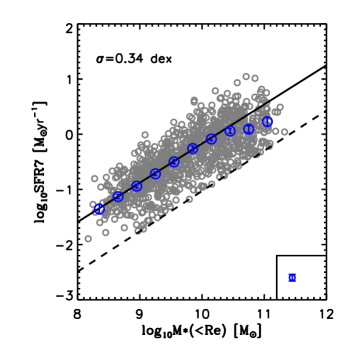
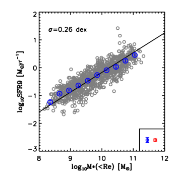
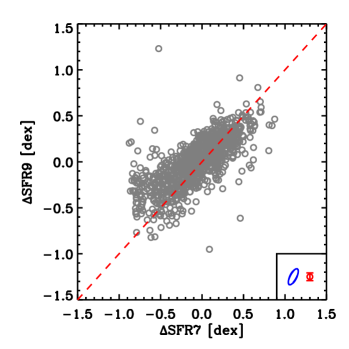
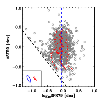
Figure 10.— Top left panel: the SFR7 versus $M_{\ast}$($<$$R_{\rm e}$) for the sample galaxies. Top right panel: the SFR9 versus $M_{\ast}$($<$$R_{\rm e}$) for the sample galaxies. In these two top panels, the blue data points are the median SFR in different stellar mass bins. The black solid line is the best-fit line to the median SFR7-$M_{\ast}$($<$$R_{\rm e}$) relation of the galaxies with $M_{\ast}$($<$$R_{\rm e}$)$<10^{10}$${\rm M}_{\odot}$, which is found to be a good description of the SFMS for SFR9. The dashed line in the left panel indicates the selection boundary of SF galaxies from W19. Bottom left panel: the $\Delta$SFR7 versus $\Delta$SFR9 for the sample galaxies. The dashed red line shows equality between these two. Bottom right panel: the $\Delta$SFR9 as a function of SFR79 for the sample galaxies. The dashed and solid red lines show the 16%, 50% and 84% of SFR79 at different $\Delta$SFR9. The vertical blue dashed lines show the overall median SFR79. The black dashed line carries over the selection criteria of SF galaxies from the top left panel. In each panel, we show the median errors (including the direction of the errors) of the data points in the corner box: the blue one is the model uncertainty, and the red one shows the uncertainty coming from the measurements from the observation. In the top left panel, the median measurement uncertainty is negligible with respect to the model uncertainty for SFR7, and therefore we do not show the typical measurement uncertainty of SFR7.

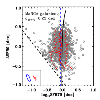
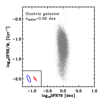
Figure 11.— The left-hand panel is the same as the bottom right panel of Figure 10, but superposes the relation of SFR79-$\Delta$SFR_800Myr that is obtained for a series of SFHs that are parallel to the evolution of the SFMS, i.e. which have constant $\Delta$SFR_800Myr, as the black solid line. The change in SFR, and thus in SFR79  due to maintaining a constant $\Delta$SFR_800Myr, is negligible. Right panel: the relation between the SFR79-SFR9/$M_{*}$ in logarithmic space for the best-fit log-normal SFHs of the SF galaxies (sSFR7 $>10^{-2}$ [Gyr^-1]) selected from Illustris from Diemer et al. (2017). Using the best-fit log-normal SFHs smooths out all short-term variations of the SFHs. For fair comparison with the left panel, we broaden the distribution of galaxies in the right panel with the typical uncertainties from both models and observations, as indicated in the bottom left-hand corner of each plot. The resulting dispersions in SFR79 are 0.08 dex and 0.23 dex respectively. This comparison emphasizes that the distribution of the observed SFR79 in MaNGA is dominated by relatively short term variations of the SFR that are absent in the log-normal SFHs.

4.1. The SFR7-based and SFR9-based SFMS

We first examine the global SFR79 and SFR9 for the sample galaxies and use these to examine the SFMS when defined using the measures of star-formation rate on the two timescales of 5 Myr and 800 Myr. Consistently with the measurements of global SFR7 (i.e. SFR_5Myr) and stellar mass, the global SFR9 is calculated for each individual galaxy by summing the flux in all the spaxels within the effective radius to obtain the integrated SFR7, SFR79 and thus SFR9 for the sample galaxies.

We exclude 16 galaxies that are located in the Seyfert regions on the Baldwin-Phillips-Telervich (BPT) diagram (Baldwin et al., 1981; Kewley et al., 2006), based on the emission line flux ratios within the effective radius, since in these galaxies the H$\alpha$ emission is largely contaminated by the contribution of the AGN. We also exclude 4 galaxies which have the three diagnostic parameters beyond the valid range of the calibrator (see details in Section 2.4). These leave 956 galaxies.

In the top two panels of Figure 10, we present the SFMS based on SFR7 (left-hand panel) and SFR9 (right-hand panel). In both panels, the blue circles show the median SFR in different stellar mass bins. The black solid line is the best-fit straight line to the median SFR7-$M_{\ast}$($<$$R_{\rm e}$) relation for galaxies with $M_{\ast}$($<$$R_{\rm e}$) less than $10^{10}$${\rm M}_{\odot}$. Following the work of W19, we define the solid line as the “nominal” SFMS for SFR7. Interestingly, the line also matches the SFMS with SFR9 very well. This is consistent with the fact that the evolution of the SFMS is small within the last 800 Myr (e.g. Brinchmann et al., 2004; Pannella et al., 2009; Stark et al., 2013; Schreiber et al., 2015) and is a reflection of the fact that our average SFR79 is very close to unity, as discussed above. We therefore adopt the solid line as the “nominal” SFMS for both SFR7 and SFR9.

The typical errors of SFR7 and SFR9, including the uncertainties from the observations and calibrator, are shown in the corner box of each panel in Figure 10. The uncertainty of SFR7 is 0.06 dex due to the conversion formula from Kennicutt (1998). The measurement uncertainty of the H$\alpha$ luminosity is negligible with respect to the uncertainty in the conversion formula to SFR, and therefore we do not show it in the top left panel. The typical uncertainty of SFR79 is 0.076 dex, obtained by combining the uncertainty from the calibrator is 0.063 dex, and the measurement error is 0.042 dex. Comparing with the intrinsic scatter within the galaxy population of SFR79 ($\sim$0.23 dex), the measurement and calibration uncertainty of SFR79 only broadens the distribution of $\log_{10}$SFR79 by less than 10%. This indicates that the dispersion of $\log_{10}$SFR79 in the bottom right panel of Figure 10 is real, which provides the basic condition to study the variability of the SFHs.

Comparing the top two panels in Figure 10, it is noticeable that the scatter of the SFMS is much smaller when using SFR9 than when using SFR7. This is to be expected. Averaging the SFR over 800 Myr eliminates the variation of SFH on shorter timescales. It should be noted that, as an extreme example of this, the SFMS would have zero scatter, if the SFR was computed as the average over the age of Universe. By examining galaxies from the EAGLE simulation, Matthee & Schaye (2019) also found that the scatter of SFMS becomes smaller when using the SFR averaged over longer timescales.

4.2. The evolution of SFMS indicated by the change parameter

Based on the “nominal” SFMS, we now define two parameters to quantify the deviation in logarithmic SFR space of each galaxy from the main-sequence at its mass, $\Delta$SFR7 and $\Delta$SFR9 (in dex) of the galaxy, i.e. the vertical distance from the “nominal” SFMS (see Figure 10). The bottom left panel of Figure 10 shows the correlation between $\Delta$SFR7 and $\Delta$SFR9.

This plot contains additional important information about how galaxies move above and below the “nominal” SFMS. An extreme scenario in which all SF galaxies evolved parallel to the “nominal” SFMS would produce $\Delta$SFR9 always equal to $\Delta$SFR7, and therefore galaxies would exactly follow the one-to-one line with zero scatter on the $\Delta$SFR7-$\Delta$SFR9 diagram. We could imagine the opposite extreme case, in which the scatter of the SFMS is purely due to the variation of SFR on very short timescales ($<<$800 Myr). In this case, we would expect that the $\Delta$SFR9 for all SF galaxies would be close to zero, and therefore galaxies would lie on a flat sequence with almost zero scatter on the $\Delta$SFR7-$\Delta$SFR9 diagram. For cases in between, galaxies would be located on a sequence with the slope between zero and one. The slope and the dispersion of the sequence on the $\Delta$SFR7-$\Delta$SFR9 diagram therefore indicates the relative contributions to the dispersion of the SFMS on long and short timescales. In the second paper of this series, we will constrain the PSD of the specific SFHs of galaxies based on the location of galaxies on the $\Delta$SFR7-$\Delta$SFR9 diagram. We do not discuss this plot further here and refer the reader to that second paper.

The bottom right panel of Figure 10 shows the relation between $\Delta$SFR9 and SFR79. The dashed and solid red lines show the 16%, 50% and 84% percentiles of SFR79 for galaxies at different $\Delta$SFR9. The lack of galaxies in the bottom-left corner is due to the fact that the definition of our SF galaxies was based on the SFR7-based SFMS (see the dashed line in the top-left panel of Figure 10). Galaxies (if any) below the dashed black line in the bottom right panel of Figure 10 would not be included in the sample selection.

As discussed above, the SFR79 parameter determines the position of a galaxy on the SFMS (defined using the SFR over the last 5 Myr), i.e. $\Delta$SFR7, relative to its position on the SFMS that is defined using the star-formation averaged over the last 800 Myr, $\Delta$SFR9. This latter quantity will to first order be the average $\Delta$SFR7 over the last 800 Myr. Therefore, apart from the small offset due to the overall evolution of the SFR in star-forming galaxies with cosmic time, the sign of SFR79 indicates whether the galaxy is generally moving up or down in sSFR (i.e. its present position relative to its average position over the last 800 Myr). Galaxies to the right of the vertical dashed line in the lower right panel of Figure 10 are in this sense increasing their sSFR, or “going up”, while those to the left are “going down” relative to the SFMS.

We have already commented that the value of $\log_{10}\langle{\rm SFR7}\rangle/\langle{\rm SFR9}\rangle$ is closely matched to the overall evolution of the sSFR of the SFMS. We furthermore here see in the lower right panel of Figure 10 that there is no apparent correlation between SFR79 and $\Delta$SFR9. The absence of a correlation between SFR79 and $\Delta$SFR9 is required if the scatter of the SFMS is to remain more or less constant over cosmic time. A strong positive correlation between $\Delta$SFR9 and SFR79 means that galaxies in the upper (lower) part of the SFMS would tend to move up (down) with respect to the “nominal” SFMS, leading over time to an increased dispersion in the SFMS. Similarly, a strong anti-correlation between $\Delta$SFR9 and SFR79, would lead to a reduced dispersion over time.

A roughly constant scatter of the SFMS is indeed seen over a wide range of cosmic epochs (e.g. Speagle et al., 2014; Whitaker et al., 2014; Schreiber et al., 2015; Barro et al., 2017), requiring that there should be no correlation between SFR79 and $\Delta$SFR9. The fact that this is indeed seen in our SFR79 estimates is an important external consistency check that provides further confirmation that our estimator for SFR79 works well.

Furthermore, it is noticeable that the distribution of SFR79, at given $\Delta$SFR9, is quite symmetrical about the median value. This symmetry is in contrast to the pronounced asymmetry in SFR79 that is visible in the bottom rightmost panel of Figure 9. In broad terms, this symmetry implies that, for an individual galaxy as a whole, the timescales of “above average star-formation” and “below average star-formation” are broadly similar. As an example, short periods of highly elevated SFR superposed on longer periods of constant SFR would produce an asymmetric distribution in SFR79 with a peak at slightly negative SFR79 and a tail to high positive SFR79. However, we do not see this in the data (the bottom right panel of Figure 10).

We return here to a point touched on earlier, namely that a galaxy with a constant sSFR will have slightly positive SFR79. This is because the SFR increases as the stellar mass increases. We show this in the left-hand panel of Figure 11 which reproduces the data from the bottom right panel of Figure 10. If all galaxies had a fixed position $\Delta$sSFR relative to the (slowly evolving) SFMS, and experienced no other variability in their (s)SFR, then they would lie precisely along the solid black line in the left panel of Figure 11, displaced to left and right only by observational scatter in determining SFR79. Because the sSFR of the SFMS is low at the current epoch, i.e. ${\rm sSFR}^{-1}>>$ 1 Gyr, the SFR79 produced by constant $\Delta$sSFR is negligible for SFMS galaxies, essentially because the mass change of the galaxy during one Gyr is negligible.

This emphasizes that the observed scatter in SFR79 within the population is completely dominated by time-variability in the SFR (and sSFR) of galaxies on timescales of 1 Gyr or less, and not by a range of (unvarying) sSFR within the population. This is further illustrated in the right hand panel of Figure 11 in which we plot the current-epoch SFR79 of the 26,485 log-normal SFH of star-forming (sSFR7 $>10^{-2}$ Gyr^-1) Illustris galaxies from Diemer et al. (2017) that were discussed above. These log-normal smooth SFH will by construction not have short-term variability. The SFR79 are computed directly from the SFH, but we add Gaussian observational scatter to the points to simulate the real data. The dispersion in SFR79 of this simulated population of log-normal galaxies is only 0.08 dex (produced almost entirely by the addition of observational uncertainties), much less than the observed dispersion of 0.23 dex. This comparison emphasizes that the much broader scatter in SFR79 in the real MaNGA data is caused by real short-term temporal variations in the SFR of galaxies that are not present in the log-normal SFH fits given by Diemer et al. (2017).

5. The spatially-resolved analysis of SFR79 

The SFR79 profile for each galaxy is constructed as in W19. We divide the spaxels for each galaxy into a set of non-overlapping elliptical annular bins with a constant radial interval in deprojected radius of $\Delta(r/Re)$=0.2. For a given galaxy, we compute the deprojected radius from the center of the galaxy based on the minor-to-major axis ratio from the NSA (NASA-Sloan Atlas) catalog (Blanton et al., 2011). Then the three diagnostic parameters, as well as the E(B-V) of the nebular emission are determined from the spaxels within each of these annuli following the approach described in Section 3.4.

Figure 12 shows the SFR79 profiles for the individual galaxies in five stellar mass bins of 0.5 dex, from $\log_{10}$($M_{\ast}(<$Re$)/$${\rm M}_{\odot}$)=8.5 to $\log_{10}$($M_{\ast}(<$Re$)/$${\rm M}_{\odot}$)=11.0. Figure 12 shows that the median SFR79 profiles (indicated by red dots) of each of the five mass sub-samples are overall flat. This is not surprising and would be expected since we applied an ad hoc $\Sigma_{*}$ adjustment as described in Section 3.3. Of more interest is the scatter in SFR79 within the population, which is shown with the red error bars. These show the dispersion $\sigma$(SFR79) computed using a three-sigma-clip algorithm. We will return to this point below.

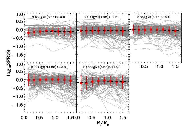
Figure 12.— The SFR79 profiles for individual MaNGA galaxies. We separate galaxies into five equal stellar mass bins in logarithmic space. In each panel, the red dots show the median SFR79 profile of the sample galaxies in the corresponding stellar mass bin. The error bars on these points indicates the 1 $\sigma$ scatter of SFR79 at a given radius.

In W19, we studied the star-formation profiles of this same sample of galaxies. Specifically, we looked at the radial elevation or suppression of the star-formation surface density (as measured on 5 Myr timescales) as a function of the overall displacement of the galaxy from the mid-line of the SFMS. We found that galaxies that are significantly above the SFMS in their overall SFR show enhanced star formation surface densities at all galactic radii and that, conversely, galaxies that are significantly below the SFMS in overall SFR show suppressed star formation surface densities at all galactic radii. Interestingly, we found that this relative enhancement (or suppression) of star formation is greater in the central regions than in the outer regions for galaxies with $\log_{10}$($M_{\ast}(<$Re$)/$${\rm M}_{\odot}$)$>$9.5.

We illustrated this further by showing (see Figure 9 of W19) that the dispersion in the radial SFR surface density at a given relative radius (for a given stellar mass bin), which we parameterized as $\sigma(\Delta\Sigma_{\rm SFR})$ in the notation of W19, strongly depended on the apparent effective gas depletion timescale. The depletion timescale was estimated using different proxies (Shi et al., 2011; Krumholz et al., 2012) rather than from a direct measure of the gas content, so the observed trend could equally well be viewed as a trend with stellar surface mass density $\Sigma_{*}^{-0.5}$ or the other proxies used in these relations.

We interpreted the W19 result as possibly reflecting the dynamical response of a gas-regulator system to changes in the gas inflow rate. We constructed a heuristic toy model in which an idealized gas-regulator (Lilly et al., 2013) was driven by a periodic inflow of different forms, either a sinusoidal function or the inverse error function. The amplitude (and to a lesser extent the phase) of the SFR response of the regulator system to this periodic variation of gas inflow varies with the ratio of the driving period and the effective gas depletion timescale, since the latter sets the response time of the regulator (see Lilly et al. (2013) for details). The observed variation of $\sigma(\Delta\Sigma_{\rm SFR})$ across galaxies and the broad features of the SFR7 profiles could therefore be explained through this simple mechanism.

We can now use the SFR79 profiles derived in the current paper to extend this result in two ways. First, rather straightforwardly, we can use the SFR79 profile to construct the $\Delta\Sigma_{\rm SFR9}$ profiles of galaxies, to complement the analysis of the $\Delta\Sigma_{\rm SFR7}$ profiles presented in W19. Second, and of more originality, we can use the SFR79 profiles to directly examine the temporal variations of SFR within galaxies. This is an important point. In W19, we interpreted the dispersion in $\Delta\Sigma_{\rm SFR}$ as arising from temporal variations in SFR, but this was precisely that: an interpretation. One could, at least in principle, imagine that galaxies evolve in such a way as to maintain a constant displacement of their overall sSFR from the mid-line of the SFMS, with a corresponding constant offset in $\Delta\Sigma_{\rm SFR7}$. In this case, the scatter of the SFMS and the scatter in star-formation surface density $\sigma(\Delta\Sigma_{\rm SFR7})$ could have nothing to do with any temporal variations in the SFR of individual galaxies, but rather reflect “intrinsic” (i.e. time-independent) differences between galaxies.

The information on SFR79 in the current work allows us to break this interpretational ambiguity decisively. Significant variations in SFR79 can only arise because of real temporal variations in the SFR within individual galaxies. It is trivial that a constant SFR in galaxies will always produce an SFR79 that is precisely unity. In the previous Section, we showed that, while a constant sSFR will produce values of SFR79 that deviate from unity, these effects are completely negligible for the sSFR of interest (see the bottom right panel of Figure 10). Unless the SFMS is a transitory phenomenon (which it is not) the scatter in SFR79 within the population is therefore completely dominated by real temporal variations of SFR (and sSFR) within individual galaxies. Therefore, if the interpretation of the $\sigma(\Delta\Sigma_{\rm SFR7})$ relation that we advanced in W19 is correct, then we should definitely expect to see a correlation between the dispersion in SFR79 with the gas depletion timescale.

In the next subsection of the paper, we construct first the $\Sigma_{\rm SFR9}$ profiles and carry out a completely analogous analysis to that of $\Sigma_{\rm SFR7}$ that was presented in W19. Then, in the subsequent subsection, we then turn to examine the SFR79 profiles for more direct information on temporal variability.

5.1. The profiles of $\Sigma_{SFR9}$

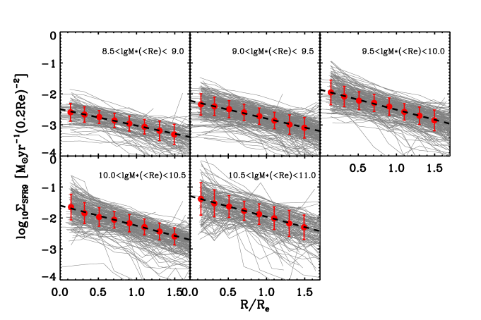
Figure 13.— The $\Sigma_{\rm SFR9}$ profiles for individual galaxies. We display the profiles in the same five stellar mass bins as in Figure 12. In each panel, the red dots show the median $\Sigma_{\rm SFR9}$ profile, and the error bars show the scatter of $\Sigma_{\rm SFR9}$ at given radii. In each panel, the dashed line is the fit of the median profile by an exponential disk.

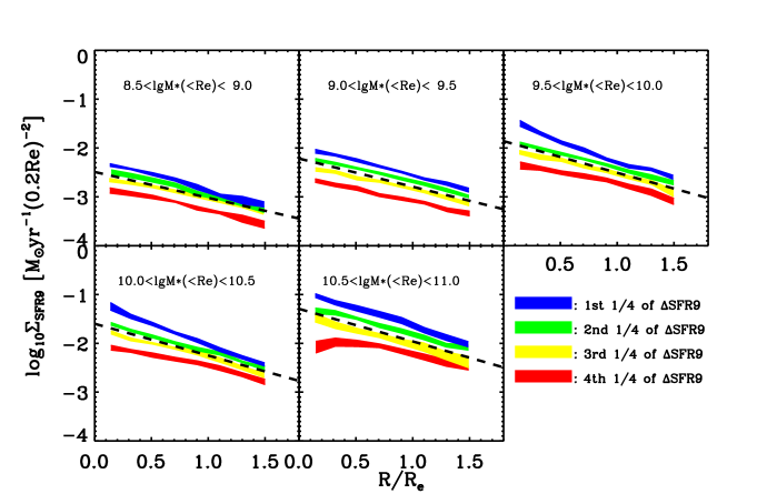
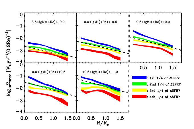
Figure 14.— Top five panels: the median $\Sigma_{\rm SFR9}$ profiles of galaxies in each quartile of $\Delta$SFR9 bins, in each of the five mass ranges. Bottom five panels: the median $\Sigma_{\rm SFR7}$ profiles for galaxies in each quartile of $\Delta$SFR7. In each stellar mass bin, we divide galaxies into four subsamples according to global $\Delta$SFR9 (or $\Delta$SFR7), i.e. the deviation from the SFR9-based (or SFR7-based) SFMS. In both sets of panels, the black dashed lines are the median profiles of all galaxies, taken from Figure 13 (or figure 4 of W19). In each panel, the thresholds of the quartiles for $\Delta$SFR7 or $\Delta$SFR9 used to separate galaxies are listed in Table 3, as well as the total number of galaxies in the corresponding stellar mass bin (the last column in Table 3).

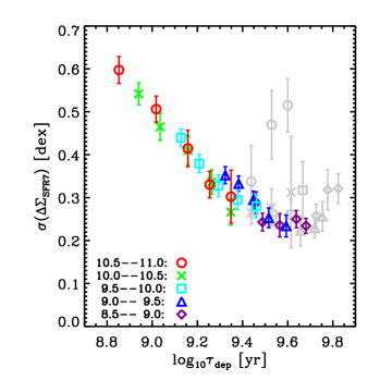
Figure 15.— Left panel: The scatter of $\Delta{\Sigma}_{\rm SFR9}$ as a function of the indirectly estimated gas depletion time. Right panel: The scatter of $\Delta{\Sigma}_{\rm SFR7}$ as a function of gas depletion time, taken from W19. In both panels, the different colors are for galaxies in different stellar mass bins, as denoted in the bottom-left corner. Data points with the radius larger than $R_{\rm e}$, are indicated in gray, as in W19.

Table 3The thresholds of the quartiles of $\Delta$SFR7, $\Delta$SFR9 and SFR79 used to classify galaxies in Figure 14 and 16.

$\log M_{*}(<Re)$		$\Delta$SFR7				$\Delta$SFR9				SFR79				Ngal
		25%	50%	75%		25%	50%	75%		25%	50%	75%
[8.5,9.0]		$-$0.134	$-$0.009	0.176		0.009	0.131	0.287		$-$0.256	$-$0.113	0.002		129
[9.0,9.5]		$-$0.219	$-$0.009	0.178		$-$0.144	0.061	0.198		$-$0.185	$-$0.068	0.067		240
[9.5,10.0]		$-$0.246	$-$0.024	0.207		$-$0.188	0.014	0.194		$-$0.140	$-$0.024	0.087		200
[10.0,10.5]		$-$0.349	$-$0.061	0.161		$-$0.231	$-$0.075	0.105		$-$0.133	$-$0.012	0.106		198
[10.5,11.0]		$-$0.502	$-$0.219	0.027		$-$0.263	$-$0.080	0.070		$-$0.300	$-$0.147	0.027		149

The profiles of $\Sigma_{\rm SFR9}$ for each individual galaxies, shown in Figure 13. For each galaxy, the $\Sigma_{\rm SFR9}$ profile is generated by combining its SFR79 profile (shown in Figure 12) and the $\Sigma_{\rm SFR7}$ profile in figure 3 of W19. When presenting the $\Sigma_{\rm SFR7}$ profiles in W19, we normalized the radius for each galaxy by dividing by the effective radius of the galaxy. This common procedure removes the effect due to the variation of galaxy size (e.g. González Delgado et al., 2016; Ellison et al., 2018; Medling et al., 2018; Guo et al., 2019). However, more originally, we also normalized the $\Sigma_{\rm SFR}$ with (0.2$R_{\rm e}$)², i.e. computed the surface density of the SFR per area of (0.2$R_{\rm e}$)². This ensures that the integration of a profile on a given surface density-radius diagram reflects the actual integrated quantity in physical terms. In the current work, we therefore present the $\Sigma_{\rm SFR9}$ profiles in the same way.

As shown in Figure 13, the $\Sigma_{\rm SFR9}$ profiles vary from galaxy to galaxy. Analogous to the result of $\Sigma_{\rm SFR7}$ profiles in W19, the scatter in $\Sigma_{\rm SFR9}$ across the galaxy population shows a larger scatter in galactic center than the outer regions ($<Re$), at least for the three highest stellar mass bins. The median profile of $\Sigma_{\rm SFR9}$ (red dots) can be well fitted by a straight line (the black dashed line), indicating a typical exponential star formation disk with no suppression of star formation (or quenching) in the central regions of galaxies. The slopes of the median $\Sigma_{\rm SFR9}$ profile are $-$0.53, $-$0.58, $-$0.65, $-$0.65 and $-$0.67 from low to high stellar mass bins, which are almost the same to the slopes of median $\Sigma_{\rm SFR7}$ profile computed in W19 at corresponding mass bins. This agrees well with the notion that star formation within main-sequence galaxies varies in a quasi-steady state within an exponential disk, ignoring other structural properties such as the presence or absence of a bulge.

We split the galaxies in each stellar mass bin into four quartiles of the global $\Delta$SFR9, i.e. the position relative to the SFMS as defined by the SFR over the last 800 Myr. The thresholds of the quartiles for $\Delta$SFR9 are listed in Table 3 for each stellar mass bin. The top set of panels in Figure 14 show the median profiles of $\Sigma_{\rm SFR9}$ for the four quartiles in global $\Delta$SFR9 for each of the five stellar mass bins. For comparison, we also evenly divide galaxies into four subsamples according to the global $\Delta$SFR7, and present their median $\Sigma_{\rm SFR7}$ profiles in the bottom panels of Figure 14. The thickness of the median profile indicates its uncertainty computed by the bootstrap method.

It can be seen from Figure 14 that galaxies with higher (or lower) global SFR9 show enhanced (or suppressed) star formation surface density (within the last 800 Myr) at all galactic radii. This elevation (or suppression) in galactic center is more pronounced in more massive galaxies. This result is entirely consistent with and analogous to the result shown in W19 for $\Sigma_{\rm SFR7}$, that galaxies with higher integrated SFR7 show higher SFR7 at all galactic radii.

Given the similar results in SFR7 and SFR9 in Figure 14, one might worry that this is somehow due to SFR9 being a derived quantity based on SFR7 and SFR79, the ratio of SFR7/SFR9. However, it is easy to see that this in fact makes the measurement of SFR9 largely independent of that of SFR7. The former is ultimately linked to the strength of H$\delta$ absorption and the latter to the strength of H$\alpha$. Clearly, if the H$\alpha$ emission due to star formation is over-estimated, for instance because of the contribution of an AGN component, then both the SFR7 and SFR79 would be more or less equally perturbed. Ultimately the value of SFR9 is based primarily on the EW(H$\delta$_A) value. The result in Figure 14 is therefore largely independent of the analogous result in W19.

W19 defined a parameter, $\Delta\Sigma_{\rm SFR7}$, to quantify the deviation from the median profile for a given stellar mass. In the same way, we now define the deviation from the median profile of $\Sigma_{\rm SFR9}$ to be $\Delta\Sigma_{\rm SFR9}$. Since the median profiles of $\Sigma_{\rm SFR7}$ have almost the same slopes of $\Sigma_{\rm SFR9}$ (and also almost the same intercepts) at all the five stellar mass bins, we use the same set of median profiles as in W19 to calculate these deviations. We note that this does not affect the measurement of the scatter of $\Delta\Sigma_{\rm SFR9}$ at a given galactic radius.

We show in Figure 15 the scatter of $\Delta\Sigma_{\rm SFR9}$ and $\Delta\Sigma_{\rm SFR7}$ (the second is taken from the right panel of figure 9 in W19 for comparison) as a function of gas depletion time. As in W19, the gas depletion time (i.e. the inverse of the star formation efficiency SFE) is calculated based on an empirical formula from Shi et al. (2011), the so-called extended-Schmidt law:

$$\frac{\rm SFE}{yr^{-1}}=10^{-10.28}\left[\frac{\Sigma_{*}}{M_{\odot}{\rm pc}^{-2}}\right]^{0.48}$$ (7)

This formula is derived from integrated observations of individual galaxies over five orders of magnitude in stellar mass density, but was found to also be valid for spiral galaxies at sub-kiloparsec resolutions and low-surface-brightness regions. In W19, we also presented another empirical formula for the gas depletion time by using the orbital timescale (Krumholz et al., 2012). Since the two give similar result, in this work we only present the one computed with the extended-Schmidt law. Each data point represents one galactic radial bin within a given galactic stellar mass bin, as in W19. The colored data points are for the radii less than $R_{\rm e}$, while gray radii are for the radii greater than $R_{\rm e}$. Here, we will only focus on those regions within the effective radius as done also in W19, because the outer regions are more likely affected by environmental effects, such as ram-pressure stripping, and etc..

Consistent with the result of W19, the scatter in $\Delta\Sigma_{\rm SFR9}$ is also evidently a decreasing function of the gas depletion time. The results on the SFR surface density on 800 Myr timescales, $\Sigma_{\rm SFR9}$, presented in this subsection extend and confirm the results on the SFR surface density on 5 Myr timescales, $\Sigma_{\rm SFR7}$, discussed in W19. The basic issue of whether variations in $\Sigma_{\rm SFR}$ reflect temporal variations or intrinsic (time-independent) differences from galaxy to galaxy however remains. To resolve this issue, we now turn to examine the SFR79 profiles more directly.

5.2. The radial profiles of SFR79 

The SFR79 profiles of the galaxies in the sample were shown in Figure 12. We now divide the galaxies in each stellar mass bin into four quartiles according to their global SFR79 as measured within their effective radii in Section 4. The top group of panels of Figure 16 shows the median SFR79 profiles of the four quartiles in overall SFR79 for each stellar mass bin. The thickness of each line reflects the uncertainty of the median SFR79 profile as computed via a bootstrap approach.

It can be seen that galaxies with high global SFR79 appear to have larger SFR79 at all galactic radii, and galaxies with low global SFR79 appear to have lower SFR79 at all galactic radii. This means that a galaxy with a certain global change in SFR, i.e. an elevation (or suppression) of the SFR with respect to the average over the last 800 Myr, experiences a corresponding elevation (or suppression) at all galactic radii. Furthermore, it can be seen that, at least for the three more massive bins of galaxy mass, this change (either elevation or suppression) is more pronounced at small galactic radii.

In the bottom panels of Figure 16, we present the analogous SFR79 profiles for the same five stellar mass bins but now dividing galaxies into four quartiles of $\Delta$SFR9, i.e. the position of the galaxies relative to the SFMS defined in terms of the SFR averaged on 800 Myr timescales. For all the mass bins, the SFR79 profiles appear to be overlapped together, independent of the $\Delta$SFR9. This means that the SFR79 profile does not depend on the location of galaxies relative to the SFR9-based SFMS. This is completely consistent with the result for the integrated SFR79 that was presented above in Section 4.2.

These results in Figures 12 and 16 are consistent but quite distinct from the result in W19. W19 found that galaxies with higher SFR with respect to the SFMS show higher SFR at all galactic radii. However, there was no direct information on the temporal changes in the SFR in W19, only an inference of spatially coherent temporal variations in the SFR. The new result in the top panels of Figure 16 allows us to look directly at these temporal changes. Galaxies with a larger (temporal) change in their overall SFR, show larger (temporal) changes in their SFR at all galactic radii. However, as shown in the bottom panels of Figure 16, we do not find larger (temporal) changes in the SFR in galaxies that have different overall levels of star-formation. This emphasizes that the SFR79 parameter, characterizing the change of SFR, gives a different perspective on galaxies than the SFR itself.

We now return to examine the dispersion in SFR79 from galaxy to galaxy at a given relative radius within a given stellar mass bin. This dispersion was shown in Figure 12 as the error bars on each point and was computed with a sigma-clipping algorithm by iteratively rejecting points beyond 3$\sigma$. For the two lowest stellar mass bins, it is evident that the scatter of SFR79 across the galaxy population does not change significantly with radius. However, for the more massive bins in stellar mass, the dispersion in SFR79 clearly increases towards the centers of galaxies relative to the scatter in the outer regions.

Since it is improbable that widely separated galaxies are varying coherently in their SFR, apart from the slow overall “cosmic” evolution of the SFMS discussed previously, the scatter in SFR79 across a population of galaxies (at a given epoch) is, as discussed earlier, unambiguously a measure of the variability of the SFR within individual objects. This is quite different from the scatter in $\Sigma_{\rm SFR7}$, which could reflect temporal changes in individual galaxies, but also, conceivably, could reflect intrinsic (time-independent) differences from galaxy to galaxy. Whereas temporal variability could only be postulated in W19 as an explanation for the correlation of $\sigma(\Delta\Sigma_{\rm SFR7})$ with the depletion time, in this paper we are able to measure temporal variability directly.

A clear predication of the gas-regulator model of Lilly et al. (2013) is that the variability of the SFR in response to variations in the inflow should strongly depend on the gas depletion time. Specifically, W19 drove the gas-regulator system with a sinusoidal inflow rate, and showed that the amplitude of the variation in the resulting SFR ($\sigma_{\rm SFR}$) is the amplitude of the variation of the inflow ($\sigma_{\rm\Phi}$) multiplied by a frequency dependent response curve. The response curve can be written as

$$f=\frac{1}{[1+(2\pi\tau_{\rm eff,dep}/\tau_{\rm P})^{2}]^{1/2}},$$ (8)

where $\tau_{\rm P}$ is the period of the cold gas inflow, and $\tau_{\rm eff,dep}$ is the “effective” gas depletion timescale, defined as the gas depletion timescale $M_{\rm gas}/{\rm SFR}$ divided by the mass-loading factor of any outflow. As shown in Equation 8, for a given inflow, a shorter $\tau_{\rm eff,dep}$ leads larger variations of SFR, and vice versa. Although Equation 8 was derived for an idealized sinusoidal input of inflow rate, similar shapes of the response curve are seen for a range of more complicated forms for the inflow rate (see details in W19).

Figure 17 shows the scatter of SFR79 at different galactic radii as a function of the inferred gas depletion time for different radii in the five stellar mass bins, computed as described in the previous subsection. In Figure 17, each data point represents one galactic radial bin at a given galactic stellar mass bin. According to Equation 7, the inner regions of galaxies correspond to the shorter gas depletion timescale.

As shown, we find that there is a tight correlation between the observed dispersion of SFR79 and the inferred gas depletion timescale, with the shorter $\tau_{\rm dep}$ associated with the larger range of SFR79. The scatter in SFR79 from galaxy to galaxy may be taken as a direct measure of the variability of the SFR in galaxies on timescales between $10^{7}$ and $10^{9}$ years.

This new result is completely independent from that presented in W19, but is entirely consistent with the heuristic model presented therein. Regions with higher SFE, i.e. with shorter depletion times, do indeed appear to show a larger response in their SFR to changes in the inflow (see figure 12 in W19). This supports the idea that the dynamical response of gas regulator model to a time-varying inflow is the origin of the variation of SFR within and across galaxies. This further supports the idea that the narrow SFMS is indeed the result of the quasi-steady state between the inflow, outflow and star formation (e.g. Schaye et al., 2010; Bouché et al., 2010; Lilly et al., 2013; Tacchella et al., 2016; Wang et al., 2019).

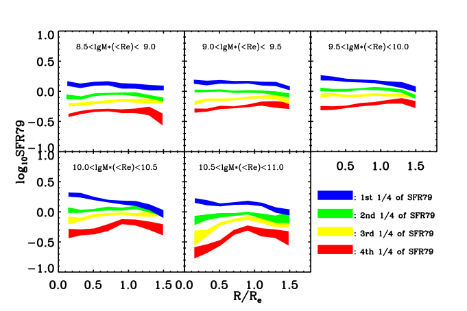
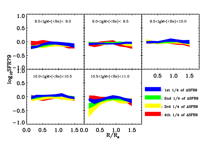
Figure 16.— Top five panels: the median SFR79 profiles for galaxies in quartiles of the overall SFR79. Bottom five panels: the median SFR79 profiles for galaxies in quartiles of the overall $\Delta$SFR9. In each stellar mass bin, the thresholds of the quartiles for SFR79 or $\Delta$SFR9 used to separate galaxies are listed in Table 3.

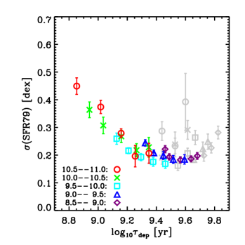
Figure 17.— The scatter of SFR79 as a function of the indirectly derived gas depletion time. The different colors are for galaxies at different stellar mass bins, as denoted in the bottom-left corner. Data points with the radius larger than $R_{\rm e}$, are indicated in gray.

5.3. Discussion

Throughout this work, we have excluded the regions that are located on the Seyfert regions on the BPT diagram in the analysis, because the contribution of H$\alpha$ emission by AGN would likely lead to an over-estimate of SFR79 (see Section 4.1). However, some inner regions of galaxies may still be contaminated by a low-luminosity AGN, although this effect must be weak for SF regions.

The connection between AGN and the instantaneous star formation has been investigated by many authors (e.g. Stanley et al., 2015, 2017; Harrison, 2017; Bernhard et al., 2018; Dai et al., 2018; Scholtz et al., 2018; Schulze et al., 2019). Although both positive and negative AGN feedback have been proposed in the literature (e.g. Silk, 2013; Bieri et al., 2016; Kalfountzou et al., 2017; Shin et al., 2019), convincing observational evidence for the impact of star formation by AGN is still lacking (Stanley et al., 2015; Bernhard et al., 2018; Ramasawmy et al., 2019; Scholtz et al., 2020). Therefore, it is not clear to us what the SFR79 profile should be for an AGN-host galaxy.

In addition to AGN, other physical processes have been proposed to play roles in changing the instantaneous SFR via different mechanisms, such as the existence of bar (e.g. Wang et al., 2012; Lin et al., 2017), and tidal/ram-pressure stripping (Gunn & Gott, 1972; Moore et al., 1996; Abadi et al., 1999; Poggianti et al., 2017). For instance, the existence of the bar can effectively transfer the cold gas to the galactic center, and lead to central enhanced star formation (Lin et al., 2017).

We emphasize that our star formation change parameter, SFR79, allows examination for the change of SFR in response to such processes. In contrast with previous studies, the SFR79 characterizes the change of star formation with respect to the level in the past, rather than to an assumed “control” population.

Many studies suggest that massive galaxies are assembled and quenched from inside outwards (e.g. Pérez et al., 2013; Tacchella et al., 2015; Abdurro’uf, 2018). Under the “inside-out” scenario, the profile of SFR79 would show a drop in the center of “quenching” or “newly quenched” galaxies (but see Lilly & Carollo (2016) for how sSFR gradients can arise without differential radial quenching). This seems at first sight consistent with the result in Figure 16, that galaxies with an overall lower SFR79 show a significant drop of SFR79 at the galactic center, at least for two highest stellar mass bins. However, we note that our galaxies are all SF galaxies as defined with the SFR7-based SFMS, which means that we may not expect to see the SFR79 profiles for newly quenched galaxies in our analysis. Instead, the SFR79 characterizes the movement of SF galaxies on the SFMS. Furthermore, analogously to our analysis in W19, galaxies with overall higher SFR79 are also seen to have elevated SFR79 in their centers.

Under the dynamical gas regulator model (Lilly et al., 2013; Wang et al., 2019), the amplitude of the change of SFR is larger for regions of short gas depletion time, and the change of SFR can be both suppression and elevation. This is also in good agreement with our result. Therefore, the drop of SFR79 in galactic center for massive galaxies with overall lower SFR79, may have little to do with quenching per se, and may be purely due to the drop of overall inflow rate.

Finally, as discussed in W19, there is no need for any specific physical processes that operate in the center to quench a galaxy “inside-out”, such as AGN feedback. Instead, the cut-off of the global inflow would naturally lead to an inside-out suppression of star-formation, due to the short gas depletion time in galaxy centers.

6. Summary and Conclusion

In this work, we have introduced and calibrated a new indicator of the change in SFR in individual galaxies, SFR79. Observationally, this is based on the equivalent widths of H$\alpha$ emission and H$\delta$ absorption, and the amplitude of the 4000 Å break. These three parameters are good indicators for recent SFHs (Worthey & Ottaviani, 1997; Kauffmann et al., 2003; Li et al., 2015; Wang et al., 2018) on different timescales. Specifically, the H$\alpha$ luminosity traces the SFH within the most recent 5 Myr, while EW(H$\delta$_A) traces the SFHs within the last $\sim$1 Gyr, and D_n(4000) is sensitive to the light-weighted stellar age within 2 Gyr.

The parameter SFR79 is equal to SFR7/SFR9, i.e. SFR_5Myr/SFR_800Myr, where the subscripts refer to the preceding time interval over which the SFR is averaged. Similarly parameters have been called burstiness in the literature (Weisz et al., 2012; Guo et al., 2016; Broussard et al., 2019), but we find this misleading in the present case. Our SFR79 spans over two orders of magnitude in timescales, which is much larger than that of UV-to-H$\alpha$ flux ratio. As distinct from the ratios of fluxes at different wavelengths, the three diagnostic spectral parameters used in the estimator of SFR79 are not in principle sensitive to dust attenuation, even if some effects can enter because of spatial variations in the extinction within galaxies. The change parameter SFR79 characterizes the changes in the SFR, in the sense that a positive (or negative) value means an elevation (or suppression) of the SFR in the last 5 Myr with respect to the average value over the last 800 Myr.

We calibrate the SFR79 by constructing millions of mock SFHs spanning a huge range of different SFR behaviours, then generating mock spectra using the SSP models for six different metallicities.

We find that SFR79 can be determined with an uncertainty of 0.06-0.09 dex for different metallicities (see Equation 2, Figure 4 and Table 1). We also examined the stability of this calibration by using a different IMF and a different stellar evolution model (i.e. isochrones). These only cause an overall shift of SFR79  and do not change the distribution (i.e. also the scatter) of the SFR79.

We compute a small second-order correction for dust attenuation that arise from a stellar age dependent E(B$-$V) model from Charlot & Fall (2000). We assume the E(B$-$V) for stellar population older than 10 Myr is the one-third of that for stellar population younger than 10 Myr (Section 2.6).

We then apply the calibrator to a well-defined sample (taken from W19) of SF main-sequence galaxies selected from the MaNGA survey, and obtain the maps and profiles of SFR79 and SFR9 for each individual galaxies, using a metallicity taken from the overall mass-metallicity relation.

Based on the new information, we investigate the variation of SFR79 and $\Sigma_{\rm SFR9}$ within and across the galaxy population. Our main results are summarized as follows.

• We have first measured the SFR79 of the whole galaxy population, i.e. the integrated (over all galaxies) SFR7 divided by the integrated SFR9. This ratio was $-$0.066 dex, reflecting a small decline in the SFR. This is remarkably close to that expected value ($-$0.025 dex) from the cosmic evolution of the characteristic sSFR of the SFMS. This reassuring agreement attests to the empirical validity of our calibration.

• We have applied a small ad hoc zero-point correction to SFR79 as a function of the stellar surface mass density, to remove a small radial dependence of SFR79 that we suspect is not real and may instead reflect an uncorrected radial dependence of the metallicity, or possibly the IMF.

• The global SFR79 (measured within $R_{\rm e}$) is nearly independent of $\Delta$SFR9, i.e. the deviation from the SFR9-based SFMS. This means that the movement of galaxies (up or down) on the SFMS does not depend on their average positions on the SFMS during the last 800 Myr. This is required if the scatter of the SFMS is to be preserved over time, as observed, since a strong positive (or negative) relation between SFR79 and $\Delta$SFR9 would broaden (or compress) the SFMS over time. This provides a further empirical support for the validity of our SFR79 estimator.

• The scatter in the SFR9-based SFMS is 0.26 dex, noticeably smaller than the SFR7-based SFMS (0.34 dex).

• Galaxies with higher (or lower) global SFR9 with respect to the “nominal” SFMS, show enhanced (or suppressed) star formation at all galactic radii with respect to median $\Sigma_{\rm SFR9}$ profile at given stellar mass. In addition, the star formation in central regions of galaxies are more enhanced (or suppressed) than outer regions (with respect to the median profile), at least for galaxies with $M_{\ast}$($<$$R_{\rm e}$)$>$9.5. These results are the equivalent for 800 Myr timescales to those already shown for the shorter 5 Myr timescales in W19.

• Of greater novelty, we show that galaxies with higher (or lower) global SFR79 appear to have higher (or lower) SFR79 at all galactic radii with, again, noticeably larger range of SFR79 in the central regions of more massive galaxies. This means that galaxies with a recent enhancement in SFR (i.e. within 5 Myr with respect to the SFR averaged over the last 800 Myr) have enhanced star formation at all galactic radii (again, with respect to the star formation in the past).

• Finally, in the most important result of the paper, we show that the dispersion in the SFR79 across the galaxy population, at a given galactic radius and stellar mass, is strongly anti-correlated with the inferred gas depletion time for these locations. The scatter in SFR79 across the population is a direct measure of the temporal variability of the SFR within individual objects, since it would be completely unreasonable to suppose that the temporal variations of widely separated galaxies are coherent (apart from a slow cosmic evolution of the SFMS).

In W19, we interpreted the observed dependence of the dispersion of $\Sigma_{\rm SFR7}$ across the population with the gas depletion timescale to be reflecting the dynamical temporal response of the gas regulator system to variations of the inflow rate. This was because, in a gas-regulator system, the amplitude of changes in the SFR to changes in the inflow rate is predicted to be strongly anti-correlated with the gas depletion time.

In the current work, we are able to measure directly these temporal changes by measuring the dispersion of the change parameter SFR79 across the population of galaxies. The fact that this dispersion is seen, once again, to anti-correlate with the inferred gas depletion timescale, further strengthens the case for the simple gas-regulation picture of galaxies and for interpreting variations in the star-formation rate of galaxies in terms of variations in the inflow rate.

The star formation change parameter proposed in this work is a new parameter, which contains valuable information of the time-varying SFH for the galaxy population. It provides a new approach to study the physical processes that govern the SFR within galaxies on different timescales. The SFR79 also opens a new window for testing models of galaxy formation and evolution in future hydrodynamical simulations and semi-analytic models. In the second paper of this series, we will explore how the power-spectrum of SFR variability in galaxies, i.e. the contribution of the variation in SFR at different timescales, based on the result in the present work.

References

- Abadi et al. (1999) Abadi, M. G., Moore, B., & Bower, R. G. 1999, MNRAS, 308, 947
- Abdurro’uf (2018) Abdurro’uf, Akiyama, M. 2018, MNRAS, 479, 5083
- Abolfathi et al. (2018) Abolfathi, B., Aguado, D. S., Aguilar, G., et al. 2018, ApJS, 235, 42
- Abramson et al. (2015) Abramson, L. E., Gladders, M. D., Dressler, A., et al. 2015, ApJ, 801, L12
- Alavi et al. (2016) Alavi, A., Siana, B., Richard, J., et al. 2016, ApJ, 832, 56
- Baldwin et al. (1981) Baldwin, J. A., Phillips, M. M., & Terlevich, R. 1981, PASP, 93, 5
- Balogh et al. (1999) Balogh, M. L., Morris, S. L., Yee, H. K. C., Carlberg, R. G., & Ellingson, E. 1999, ApJ, 527, 54
- Barro et al. (2017) Barro, G., Faber, S. M., Koo, D. C., et al. 2017, ApJ, 840, 47
- Bernhard et al. (2018) Bernhard, E., Mullaney, J. R., Aird, J., et al. 2018, MNRAS, 476, 436
- Bertelli et al. (1994) Bertelli, G., Bressan, A., Chiosi, C., Fagotto, F., & Nasi, E. 1994, A&AS, 106, 275
- Bertelli et al. (2008) Bertelli, G., Girardi, L., Marigo, P., & Nasi, E. 2008, A&A, 484, 815
- Bieri et al. (2016) Bieri, R., Dubois, Y., Silk, J., Mamon, G. A., & Gaibler, V. 2016, MNRAS, 455, 4166
- Blanton et al. (2011) Blanton, M. R., Kazin, E., Muna, D., Weaver, B. A., & Price-Whelan, A. 2011, AJ, 142, 31
- Blitz & Shu (1980) Blitz, L., & Shu, F. H. 1980, ApJ, 238, 148
- Boogaard et al. (2018) Boogaard, L. A., Brinchmann, J., Bouché, N., et al. 2018, A&A, 619, A27
- Boselli et al. (2009) Boselli, A., Boissier, S., Cortese, L., et al. 2009, ApJ, 706, 1527
- Bouché et al. (2010) Bouché, N., Dekel, A., Genzel, R., et al. 2010, ApJ, 718, 1001
- Bouwens et al. (2011) Bouwens, R. J., Illingworth, G. D., Oesch, P. A., et al. 2011, ApJ, 737, 90
- Bouwens et al. (2014) Bouwens, R. J., Bradley, L., Zitrin, A., et al. 2014, ApJ, 795, 126
- Brinchmann et al. (2004) Brinchmann, J., Charlot, S., White, S. D. M., et al. 2004, MNRAS, 351, 1151
- Broussard et al. (2019) Broussard, A., Gawiser, E., Iyer, K., et al. 2019, ApJ, 873, 74
- Bruzual & Charlot (2003) Bruzual, G., & Charlot, S. 2003, MNRAS, 344, 1000
- Bruzual A. (1983) Bruzual A., G. 1983, ApJ, 273, 105
- Bundy et al. (2015) Bundy, K., Bershady, M. A., Law, D. R., et al. 2015, ApJ, 798, 7
- Byler et al. (2017) Byler, N., Dalcanton, J. J., Conroy, C., & Johnson, B. D. 2017, ApJ, 840, 44
- Calzetti et al. (2000) Calzetti, D., Armus, L., Bohlin, R. C., et al. 2000, ApJ, 533, 682
- Caplar & Tacchella (2019) Caplar, N., & Tacchella, S. 2019, MNRAS, 487, 3845
- Cardelli et al. (1989) Cardelli, J. A., Clayton, G. C., & Mathis, J. S. 1989, ApJ, 345, 245
- Carnall et al. (2019) Carnall, A. C., Leja, J., Johnson, B. D., et al. 2019, ApJ, 873, 44
- Ceverino & Klypin (2009) Ceverino, D., & Klypin, A. 2009, ApJ, 695, 292
- Chabrier (2003) Chabrier, G. 2003, PASP, 115, 763
- Charlot & Fall (2000) Charlot, S., & Fall, S. M. 2000, ApJ, 539, 718
- Choi et al. (2016) Choi, J., Dotter, A., Conroy, C., et al. 2016, ApJ, 823, 102
- Chown et al. (2019) Chown, R., Li, C., Athanassoula, E., et al. 2019, MNRAS, 484, 5192
- Cid Fernandes et al. (2004) Cid Fernandes, R., Gu, Q., Melnick, J., et al. 2004, MNRAS, 355, 273
- Cignoni et al. (2015) Cignoni, M., Sabbi, E., van der Marel, R. P., et al. 2015, ApJ, 811, 76
- Conroy (2013) Conroy, C. 2013, ARA&A, 51, 393
- Conroy et al. (2009) Conroy, C., Gunn, J. E., & White, M. 2009, ApJ, 699, 486
- Daddi et al. (2007) Daddi, E., Dickinson, M., Morrison, G., et al. 2007, ApJ, 670, 156
- Dai et al. (2018) Dai, Y. S., Wilkes, B. J., Bergeron, J., et al. 2018, MNRAS, 478, 4238
- Davé et al. (2011) Davé, R., Oppenheimer, B. D., & Finlator, K. 2011, MNRAS, 415, 11
- Davies et al. (2019) Davies, L. J. M., Lagos, C. d. P., Katsianis, A., et al. 2019, MNRAS, 483, 1881
- Dekel & Burkert (2014) Dekel, A., & Burkert, A. 2014, MNRAS, 438, 1870
- Diemer et al. (2017) Diemer, B., Sparre, M., Abramson, L. E., & Torrey, P. 2017, ApJ, 839, 26
- Dotter (2016) Dotter, A. 2016, ApJS, 222, 8
- Dressler et al. (2013) Dressler, A., Oemler, Augustus, J., Poggianti, B. M., et al. 2013, ApJ, 770, 62
- El-Badry et al. (2016) El-Badry, K., Wetzel, A., Geha, M., et al. 2016, ApJ, 820, 131
- Elbaz et al. (2007) Elbaz, D., Daddi, E., Le Borgne, D., et al. 2007, A&A, 468, 33
- Elbaz et al. (2011) Elbaz, D., Dickinson, M., Hwang, H. S., et al. 2011, A&A, 533, A119
- Ellison et al. (2018) Ellison, S. L., Sánchez, S. F., Ibarra-Medel, H., et al. 2018, MNRAS, 474, 2039
- Emami et al. (2019) Emami, N., Siana, B., Weisz, D. R., et al. 2019, ApJ, 881, 71
- Faisst et al. (2019) Faisst, A. L., Capak, P. L., Emami, N., Tacchella, S., & Larson, K. L. 2019, ApJ, 884, 133
- Falcón-Barroso et al. (2011) Falcón-Barroso, J., Sánchez-Blázquez, P., Vazdekis, A., et al. 2011, A&A, 532, A95
- Ferland et al. (2013) Ferland, G. J., Porter, R. L., van Hoof, P. A. M., et al. 2013, RMxAA, 49, 137
- Freeman et al. (2017) Freeman, P., Rosolowsky, E., Kruijssen, J. M. D., Bastian, N., & Adamo, A. 2017, MNRAS, 468, 1769
- Gallazzi & Bell (2009) Gallazzi, A., & Bell, E. F. 2009, ApJS, 185, 253
- Ge et al. (2018) Ge, J., Yan, R., Cappellari, M., et al. 2018, MNRAS, 478, 2633
- Gladders et al. (2013) Gladders, M. D., Oemler, A., Dressler, A., et al. 2013, ApJ, 770, 64
- Goddard et al. (2017) Goddard, D., Thomas, D., Maraston, C., et al. 2017, MNRAS, 466, 4731
- González Delgado et al. (2016) González Delgado, R. M., Cid Fernandes, R., Pérez, E., et al. 2016, A&A, 590, A44
- Goto et al. (2019) Goto, T., Oi, N., Utsumi, Y., et al. 2019, PASJ, 71, 30
- Gunawardhana et al. (2011) Gunawardhana, M. L. P., Hopkins, A. M., Sharp, R. G., et al. 2011, MNRAS, 415, 1647
- Gunn & Gott (1972) Gunn, J. E., & Gott, J. Richard, I. 1972, ApJ, 176, 1
- Guo et al. (2019) Guo, K., Peng, Y., Shao, L., et al. 2019, ApJ, 870, 19
- Guo et al. (2016) Guo, Y., Rafelski, M., Faber, S. M., et al. 2016, ApJ, 833, 37
- Hagen et al. (2015) Hagen, L. M. Z., Hoversten, E. A., Gronwall, C., et al. 2015, ApJ, 808, 178
- Harrison (2017) Harrison, C. M. 2017, Nature Astronomy, 1, 0165
- Hemmati et al. (2015) Hemmati, S., Mobasher, B., Darvish, B., et al. 2015, ApJ, 814, 46
- Hollyhead et al. (2015) Hollyhead, K., Bastian, N., Adamo, A., et al. 2015, MNRAS, 449, 1106
- Kalfountzou et al. (2017) Kalfountzou, E., Stevens, J. A., Jarvis, M. J., et al. 2017, MNRAS, 471, 28
- Kashino et al. (2013) Kashino, D., Silverman, J. D., Rodighiero, G., et al. 2013, ApJ, 777, L8
- Kauffmann et al. (2003) Kauffmann, G., Heckman, T. M., White, S. D. M., et al. 2003, MNRAS, 341, 33
- Kennicutt (1998) Kennicutt, Robert C., J. 1998, ARA&A, 36, 189
- Kewley et al. (2006) Kewley, L. J., Groves, B., Kauffmann, G., & Heckman, T. 2006, MNRAS, 372, 961
- Klypin et al. (2016) Klypin, A., Yepes, G., Gottlöber, S., Prada, F., & Heß, S. 2016, MNRAS, 457, 4340
- Krumholz et al. (2012) Krumholz, M. R., Dekel, A., & McKee, C. F. 2012, ApJ, 745, 69
- Law et al. (2016) Law, D. R., Cherinka, B., Yan, R., et al. 2016, AJ, 152, 83
- Leja et al. (2019) Leja, J., Carnall, A. C., Johnson, B. D., Conroy, C., & Speagle, J. S. 2019, ApJ, 876, 3
- Li et al. (2005) Li, C., Wang, T.-G., Zhou, H.-Y., Dong, X.-B., & Cheng, F.-Z. 2005, AJ, 129, 669
- Li et al. (2015) Li, C., Wang, E., Lin, L., et al. 2015, ApJ, 804, 125
- Lilly & Carollo (2016) Lilly, S. J., & Carollo, C. M. 2016, ApJ, 833, 1
- Lilly et al. (2013) Lilly, S. J., Carollo, C. M., Pipino, A., Renzini, A., & Peng, Y. 2013, ApJ, 772, 119
- Lilly et al. (1996) Lilly, S. J., Le Fevre, O., Hammer, F., & Crampton, D. 1996, ApJ, 460, L1
- Lin et al. (2017) Lin, L., Li, C., He, Y., Xiao, T., & Wang, E. 2017, ApJ, 838, 105
- Lin & Kong (2019) Lin, Z., & Kong, X. 2019, arXiv e-prints, arXiv:1912.01851
- Madau & Dickinson (2014) Madau, P., & Dickinson, M. 2014, ARA&A, 52, 415
- Matthee & Schaye (2019) Matthee, J., & Schaye, J. 2019, MNRAS, 484, 915
- Medling et al. (2018) Medling, A. M., Cortese, L., Croom, S. M., et al. 2018, MNRAS, 475, 5194
- Moore et al. (1996) Moore, B., Katz, N., Lake, G., Dressler, A., & Oemler, A. 1996, Nature, 379, 613
- Moustakas & Kennicutt (2006) Moustakas, J., & Kennicutt, Robert C., J. 2006, ApJS, 164, 81
- Muratov et al. (2015) Muratov, A. L., Kereš, D., Faucher-Giguère, C.-A., et al. 2015, MNRAS, 454, 2691
- Murray et al. (2010) Murray, N., Quataert, E., & Thompson, T. A. 2010, ApJ, 709, 191
- Muzzin et al. (2009) Muzzin, A., Marchesini, D., van Dokkum, P. G., et al. 2009, ApJ, 701, 1839
- Noeske et al. (2007) Noeske, K. G., Weiner, B. J., Faber, S. M., et al. 2007, ApJ, 660, L43
- Ocvirk et al. (2006) Ocvirk, P., Pichon, C., Lançon, A., & Thiébaut, E. 2006, MNRAS, 365, 46
- Oemler et al. (2013) Oemler, Augustus, J., Dressler, A., Gladders, M. G., et al. 2013, ApJ, 770, 63
- Osterbrock & Ferland (2006) Osterbrock, D. E., & Ferland, G. J. 2006
- Pannella et al. (2009) Pannella, M., Gabasch, A., Goranova, Y., et al. 2009, ApJ, 701, 787
- Papovich et al. (2001) Papovich, C., Dickinson, M., & Ferguson, H. C. 2001, ApJ, 559, 620
- Paxton et al. (2011) Paxton, B., Bildsten, L., Dotter, A., et al. 2011, ApJS, 192, 3
- Paxton et al. (2018) Paxton, B., Schwab, J., Bauer, E. B., et al. 2018, ApJS, 234, 34
- Peng et al. (2010) Peng, Y.-j., Lilly, S. J., Kovač, K., et al. 2010, ApJ, 721, 193
- Pérez et al. (2013) Pérez, E., Cid Fernandes, R., González Delgado, R. M., et al. 2013, ApJ, 764, L1
- Poggianti et al. (2017) Poggianti, B. M., Moretti, A., Gullieuszik, M., et al. 2017, ApJ, 844, 48
- Pozzetti et al. (2010) Pozzetti, L., Bolzonella, M., Zucca, E., et al. 2010, A&A, 523, A13
- Ramasawmy et al. (2019) Ramasawmy, J., Stevens, J., Martin, G., & Geach, J. E. 2019, MNRAS, 486, 4320
- Reddy et al. (2015) Reddy, N. A., Kriek, M., Shapley, A. E., et al. 2015, ApJ, 806, 259
- Rodríguez-Puebla et al. (2016) Rodríguez-Puebla, A., Primack, J. R., Behroozi, P., & Faber, S. M. 2016, MNRAS, 455, 2592
- Sacchi et al. (2019) Sacchi, E., Cignoni, M., Aloisi, A., et al. 2019, ApJ, 878, 1
- Salpeter (1955) Salpeter, E. E. 1955, ApJ, 121, 161
- Sánchez-Blázquez et al. (2006) Sánchez-Blázquez, P., Peletier, R. F., Jiménez-Vicente, J., et al. 2006, MNRAS, 371, 703
- Schaye et al. (2010) Schaye, J., Dalla Vecchia, C., Booth, C. M., et al. 2010, MNRAS, 402, 1536
- Schiminovich et al. (2005) Schiminovich, D., Ilbert, O., Arnouts, S., et al. 2005, ApJ, 619, L47
- Scholtz et al. (2018) Scholtz, J., Alexander, D. M., Harrison, C. M., et al. 2018, MNRAS, 475, 1288
- Scholtz et al. (2020) Scholtz, J., Harrison, C. M., Rosario, D. J., et al. 2020, MNRAS, 51
- Schreiber et al. (2015) Schreiber, C., Pannella, M., Elbaz, D., et al. 2015, A&A, 575, A74
- Schulze et al. (2019) Schulze, A., Silverman, J. D., Daddi, E., et al. 2019, MNRAS, 488, 1180
- Shapley et al. (2001) Shapley, A. E., Steidel, C. C., Adelberger, K. L., et al. 2001, ApJ, 562, 95
- Shapley et al. (2005) Shapley, A. E., Steidel, C. C., Erb, D. K., et al. 2005, ApJ, 626, 698
- Shi et al. (2011) Shi, Y., Helou, G., Yan, L., et al. 2011, ApJ, 733, 87
- Shin et al. (2019) Shin, J., Woo, J.-H., Chung, A., et al. 2019, ApJ, 881, 147
- Silk (2013) Silk, J. 2013, ApJ, 772, 112
- Sparre et al. (2017) Sparre, M., Hayward, C. C., Feldmann, R., et al. 2017, MNRAS, 466, 88
- Sparre et al. (2015) Sparre, M., Hayward, C. C., Springel, V., et al. 2015, MNRAS, 447, 3548
- Speagle et al. (2014) Speagle, J. S., Steinhardt, C. L., Capak, P. L., & Silverman, J. D. 2014, ApJS, 214, 15
- Stanley et al. (2015) Stanley, F., Harrison, C. M., Alexander, D. M., et al. 2015, MNRAS, 453, 591
- Stanley et al. (2017) Stanley, F., Alexander, D. M., Harrison, C. M., et al. 2017, MNRAS, 472, 2221
- Stark et al. (2013) Stark, D. P., Schenker, M. A., Ellis, R., et al. 2013, ApJ, 763, 129
- Sullivan et al. (2000) Sullivan, M., Treyer, M. A., Ellis, R. S., et al. 2000, MNRAS, 312, 442
- Tacchella et al. (2016) Tacchella, S., Dekel, A., Carollo, C. M., et al. 2016, MNRAS, 457, 2790
- Tacchella et al. (2015) Tacchella, S., Carollo, C. M., Renzini, A., et al. 2015, Science, 348, 314
- Tolstoy et al. (2009) Tolstoy, E., Hill, V., & Tosi, M. 2009, ARA&A, 47, 371
- Wang et al. (2017) Wang, E., Kong, X., Wang, H., et al. 2017, ApJ, 844, 144
- Wang et al. (2019) Wang, E., Lilly, S. J., Pezzulli, G., & Matthee, J. 2019, ApJ, 877, 132
- Wang et al. (2018) Wang, E., Li, C., Xiao, T., et al. 2018, ApJ, 856, 137
- Wang et al. (2012) Wang, J., Kauffmann, G., Overzier, R., et al. 2012, MNRAS, 423, 3486
- Weisz et al. (2012) Weisz, D. R., Johnson, B. D., Johnson, L. C., et al. 2012, ApJ, 744, 44
- Whitaker et al. (2012) Whitaker, K. E., van Dokkum, P. G., Brammer, G., & Franx, M. 2012, ApJ, 754, L29
- Whitaker et al. (2014) Whitaker, K. E., Franx, M., Leja, J., et al. 2014, ApJ, 795, 104
- Wild et al. (2011) Wild, V., Charlot, S., Brinchmann, J., et al. 2011, MNRAS, 417, 1760
- Worthey et al. (1994) Worthey, G., Faber, S. M., Gonzalez, J. J., & Burstein, D. 1994, ApJS, 94, 687
- Worthey & Ottaviani (1997) Worthey, G., & Ottaviani, D. L. 1997, ApJS, 111, 377
- Wuyts et al. (2011) Wuyts, S., Förster Schreiber, N. M., van der Wel, A., et al. 2011, ApJ, 742, 96
- Zahid et al. (2017) Zahid, H. J., Kudritzki, R.-P., Conroy, C., Andrews, B., & Ho, I. T. 2017, ApJ, 847, 18
- Zhang et al. (2018) Zhang, Z.-Y., Romano, D., Ivison, R. J., Papadopoulos, P. P., & Matteucci, F. 2018, Nature, 558, 260
- Zheng et al. (2017) Zheng, Z., Wang, H., Ge, J., et al. 2017, MNRAS, 465, 4572
- Zibetti et al. (2009) Zibetti, S., Charlot, S., & Rix, H.-W. 2009, MNRAS, 400, 1181
- Zolotov et al. (2015) Zolotov, A., Dekel, A., Mandelker, N., et al. 2015, MNRAS, 450, 2327