Dynamics of Open Tight-binding Model

Abstract

In this paper, we investigate the open tight-binding model with $N$ sites coupled to two reservoirs on its edges with the nonequilibrium Green function method to understand effects of open boundaries. As a result, we obtain an analytical expression of the electron density in the steady state and in the transient regime for $N\rightarrow\infty$ and at absolute zero temperature. From the expression of the electron density in the steady state, we show that the open boundaries do not affect the qualitative behavior of the electron density and the phase transition which has been observed for the isolated tight-binding model also exists in our open case. Using the expression of the time-dependent electron density, we show that a two-step decay appears in the relaxation process purely caused by open boundaries. In addition, we show that the dependence of speed of convergence on boundary coupling strength qualitatively changes at a certain value of the boundary parameters. This is a result of special eigenvalues of a non-hermitian matrix whose imaginary parts do not vanish even in the limit $N\rightarrow\infty$.

1 Introduction

With recent remarkable developments of creating and manipulating experimental systems such as cold atomic system[1, 2], open quantum systems have been investigated extensively. Especially, low-dimensional open quantum system is a field of interest, where we have found interesting phenomena such as nonequilibrium phase transitions by dissipation[3, 4, 5, 6] and topological phase transitions[7, 8].

To investigate low-dimensional open quantum systems, two approaches have been mainly used. One approach is known as Quantum Master Equation(QME)[9, 10], a differential equation of the density operator of a subsystem derived by reducing the freedom of reservoirs from the density operator of the total system and using several approximations such as Markov reservoir. With QME, many low-dimensional spin systems have been studied[11, 12, 13, 14, 15, 16, 17, 18, 19, 20]. Especially, analysis has been carried out for steady state in one-dimensional systems with the matrix ansatz[11, 12, 13, 14]. In these papers, the authors studied one-dimensional open XX and XXZ spin chain in the steady state and obtained analytical expressions for physical quantities such as correlation functions. For details, see a review[14]. In the case of transient dynamics, analytical understanding is less satisfactory than the steady case[15, 16, 17, 18, 19, 20]. In [17], the author studied the dependence of the system size to relaxation time in XX and XXZ spin models with dephasing. The spectrum of the Lindblad operator in several spin models with dephasing has been studied[18, 19, 20], but the analytical understanding of transient dynamics with dissipation caused by reservoir has remained to be investigated.

The other method to explore the nonequilibrium state of open quantum system is the nonequilibrium Green function method(NEGF)[21, 22]. The method is an extension of the standard Green function method so that one can use the diagram techniques even for nonequilibrium systems. In contrast to QME, NEGF does not tell us information of the density matrix itself about system which we focus on. However, understanding of transient dynamics is relatively progressing[23, 24, 25, 26, 27, 28, 29, 30]. At the beginning, NEGF did not include the effect of the initial correlation between the system and reservoirs, which could not be ignored when we focus on the transient dynamics. A further extension was accomplished to include the initial correlation in [23, 24]. Using the formula, dynamics of general systems has been studied [25, 26, 27, 28]. In the study[25], the authors paved the way for calculating the Green functions including the effects of the Coulomb interaction using proper approximation of the self-energy to conserve physical quantities such as energy. Recently, more efficient way of computing one-body physical quantity has been used with the generalized Kadanoff-Baym ansatz[31, 30]. Without the Coulomb interaction, transport properties were calculated exactly[26] in the wide-band-limit approximation (WBLA). The method of calculation in [26] has been employed to study the case where an arbitrary time-dependent bias is applied to reservoirs[27, 28] and to investigate double quantum dots[29]. However, the application of general results in NEGF to concrete systems has not been enough.

In this paper, to obtain further understanding about dynamics of low-dimensional open quantum systems, we investigate the open tight-binding model coupled to two reservoirs on its edges with the NEGF method including initial effect. It is worth studying this model from two reasons. Theoretically, dynamics of the isolated tight-binding model, or equivalently XX model which is obtained by Jordan-Wigner transformation, has been studied extensively[32, 33, 34, 35] and we can observe interesting phenomena such as scaling behavior of magnetization[32]. Therefore, we can expect further rich behaviors in the open case due to boundary effects. In addition, this model can be implemented experimentally by using cold atomic systems[36, 37]. Hence we can testify our results from experimental points of view. As a result, we obtain an analytical expression of the electron density in the steady state and in the transient regime for $N\rightarrow\infty$ and at absolute zero temperature, which we use to mimic the situation of the experiment. From the expression of the electron density in the steady state, we can prove a phase transition, whose transition point is the same as that obtained in the isolated case[38], exists in our open case. In addition, we show that the boundary parameters do not change the qualitative behavior of the electron density in the steady state. In contrast, we can see boundary effects in the transient regime. We analytically understand that the time-dependent electron density has a two-step decay in the region where the on-site energy is not large enough and boundary couplings exist as Fig. 15 shows. This phenomenon is purely caused by boundary parameters. We also show that the dependence of speed of convergence to steady state on the boundary couplings changes at a certain value (Fig. 17). It is reasonable to consider that the speed of convergence increase as the couplings on the boundaries become large because the couplings determine how easily particles from reservoirs can flow into the sites. However, contrary to the expectation, the dependence actually changes at certain values of the coupling constants and the speed decreases as the couplings become large. This is caused by special eigenvalues, whose imaginary part does not vanish even in the limit $N\rightarrow\infty$, of a non-hermitian matrix in the expression of the electron density. Because the values of the boundary parameters determine the existence of the special eigenvalues, the qualitative change in the behavior of the time-dependent electron density is a result of the open boundaries.

This paper is organized as follows. In Sect. 2, we briefly review the previous results obtained with the NEGF method including the initial correlation effect. By considering the result in our case, we can obtain a formal expression for the time-dependent electron density of site $n$. In Sect. 3, we show several natures of the non-hermitian matrix, an important quantity of one-body physical quantities. Especially, we investigate special eigenvalues of the non-hermitian matrix. We need to pay attention to the special eigenvalues when we analyze physical quantities because the eigenvalues change the expressions of the quantities. Based on the understandings, we examine the behavior of the electron density in the steady state and the transient regime in Sect. 4 and Sect. 5. In Sect. 4, we study the electron density in steady state and obtain a simple expression of the electron density. From the expression, we show the existence of a phase transition and the boundary parameters do not affect the qualitative behavior of the electron density in the steady state. We investigate the time-dependent electron density in Sect. 5. From the analytical expression of the time-dependent electron density, we show the existence of a two-step decay and consider the physical understanding of the behavior. We also find that the dependence of speed of convergence to steady state on the boundary coupling constants changes at a certain value. Sect. 6 is the conclusion of this study.

2 Our model and prevoirs results

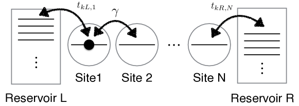
Fig. 1: Schematic diagram of our system.

Our model is the straightly connected $N$ tight-binding model coupled to two reservoirs(Fig. 1). We consider the case where each site has a single energy level. Therefore, a single electron can exist in each site when we ignore the freedom of spin. The discussion can be extended to the case including the freedom of spin straightforwardly. We assume that, initially at time $t=0$, the sites and the reservoirs are in the thermal-equilibrium state characterized by an inverse temperature $\beta$ and a chemical potential $\mu$. Then for $t>0$, a constant bias voltage $V_{\alpha}$ is applied to the reservoir $\alpha=\{\mathrm{L},\mathrm{R}\}$ and the system gets into a nonequilibrium state. The Hamiltonian of total system with $N$ sites is represented as

$$H(t)=\\ \begin{cases}\sum_{\alpha=\{L,R\},k\alpha}(\epsilon_{k\alpha}-\mu)d^{\dagger}_{k\alpha}d_{k\alpha}+\sum^{N}_{n=1}(\epsilon-\mu)d^{\dagger}_{n}d_{n}+V_{1L}+V_{NR}+\sum^{N-1}_{i=1}T_{n,n+1},&t<t_{0}\\ \sum_{\alpha=\{L,R\},k\alpha}(\epsilon_{k\alpha}+V_{\alpha})d^{\dagger}_{k\alpha}d_{k\alpha}+\sum^{N}_{n=1}\epsilon d^{\dagger}_{n}d_{n}+V_{1L}+V_{NR}+\sum^{N-1}_{n=1}T_{n,n+1},&t\geq t_{0}\end{cases}$$ (1)

where $\epsilon_{k\alpha}$ is the $k$th eigenvalue of the Hamiltonian of reservoir $\alpha$ and $\epsilon$ is the on-site energy of the sites. $d_{k\alpha},d^{\dagger}_{k\alpha}$ are the creation and the annihilation operators of reservoir $\alpha$ and $d_{n},d^{\dagger}_{n}$ are those of site $n$. The transported particles are Fermion and thus the operators satisfy the anti-commutation relations: $\{d_{i},d^{\dagger}_{j}\}=\delta_{ij}$, $\{d_{i},d_{j}\}=\{d^{\dagger}_{i},d^{\dagger}_{j}\}=0$. Each term of the Hamiltonian has the meaning as follows: the first term is the (diagonalized) Hamiltonian of the reservoirs, the second is the Hamiltonian of the sites, the third is the coupling between site 1 and the left reservoir, the fourth is the coupling between site $N$ and the right reservoir. The fifth is the coupling between the sites. Here, we assume the couplings are written in the forms:

$$V_{i\alpha}=\sum_{k\alpha}t_{k\alpha,i}d^{\dagger}_{k\alpha}d_{i}+t_{i,k\alpha}d^{\dagger}_{i}d_{k\alpha}\ (i=1,N),$$

$$T_{n,n+1}=\gamma d^{\dagger}_{n+1}d_{n}+\gamma d^{\dagger}_{n}d_{n+1}\ (n=1,2,\cdots N-1).$$

This means we consider the case where Coulomb interaction is negligible. Experimentally, this approximation may be justified when the energy scale of electrons is larger than that of the Coulomb interaction such as a high bias voltage.

In this situation, we want to know the quantitative behavior in the steady state and the transient dynamics. To investigate this, we calculate the electron density at site $i$ defined as $\rho_{i}(t):=\braket{d^{\dagger}_{H,i}(t)d_{H,i}(t)}$. One of the methods to calculate physical quantities in nonequilibrium state is NEGF. Until now, with the NEGF and WBLA, the expression of the Green function, which is the basic quantity for one-body physical quantities, has been obtained in general situations without Coulomb interaction[26, 27]. Here WBLA means that the energy bands of reservoirs are so wide and only the electrons on the Fermi energy are transported. We use a formal expression of time-dependent electron density $\rho_{n}(t)$ at site $n$ in [26] written as

$$\rho_{n}(t) =\big{[}\sum_{\alpha=\{L,R\}}\int^{\infty}_{-\infty}\frac{d\omega}{2\pi}f(\omega-\mu)\mathbf{\Lambda}_{\alpha}(\omega+V_{\alpha})$$

$$+V_{\alpha}(e^{-i\mathbf{h}^{eff}(t-t_{0})}\mathbf{G}^{r}(\omega)\mathbf{\Lambda}_{\alpha}(\omega+V_{\alpha})e^{i(\omega+V_{\alpha})(t-t_{0})}+\mathrm{H.c.})$$

$$+V^{2}_{\alpha}e^{-i\mathbf{h}^{eff}(t-t_{0})}\mathbf{G}^{r}(\omega)\mathbf{\Lambda}_{\alpha}(\omega+V_{\alpha})\mathbf{G}^{a}(\omega)e^{i(\mathbf{h}^{eff})^{*}(t-t_{0})}\big{]}_{nn},$$ (2)

where $\mathbf{\Lambda}_{\alpha}=\mathbf{G}^{r}(\omega)\Gamma_{\alpha}\mathbf{G}^{a}(\omega)$ is a spectral function and $f(\omega)=\{1+e^{\beta\omega}\}^{-1}$ is the Fermi distribution function. In the following analysis, we set the chemical potential $\mu$ to be 0 because $\mu$ is just a shift of energy. $\mathbf{G}^{r}(\omega)=\{\omega\mathbf{1}_{N}-\mathbf{h}^{eff}\}^{-1}$ and $\mathbf{G}^{a}(\omega)=\{\omega\mathbf{1}_{N}-(\mathbf{h}^{eff})^{*}\}^{-1}$ are the retarded Green function and the advanced Green function respectively. Here $\mathbf{h}^{eff}=\mathbf{h}-\frac{i}{2}\mathbf{\Gamma}$ is a non-hermitian matrix including the effect from the reservoirs and representing the geometrical configuration of the sites. Depending on the form of the hamiltonian and couplings between sites and reservoirs, the expression of $\mathbf{h}^{eff}$ changes. In our case of (1), each term of the non-hermitian matrix is defined as follows. $\mathbf{\Gamma}=\sum_{\alpha}\mathbf{\Gamma}_{\alpha}$ and $\mathbf{\Gamma}_{\alpha}$ is the matrix which expresses the coupling between the sites and the reservoir $\alpha$. These matrices take the following forms in our case:

$$\left[\mathbf{\Gamma}_{L}\right]_{nm}=\begin{cases}\Gamma_{L},&n=m=1,\\ 0,&\mathrm{else},\end{cases} \left[\mathbf{\Gamma}_{R}\right]_{ij}=\begin{cases}\Gamma_{R},&i=j=N,\\ 0,&\mathrm{else}.\end{cases}$$ (3)

The expression of the matrix $\mathbf{\Gamma}_{\alpha}$ changes depending on the couplings between the sites and reservoirs. Because the left reservoir only connects with the site 1 in our case, $\mathbf{\Gamma}_{L}$ has only the non-zero value $\Gamma_{L}$ at $(1,1)$ component. Similarly, $\mathbf{\Gamma}_{R}$ only has the non-zero value $\Gamma_{R}$ at $(N,N)$ component. We note that the parameters $t_{k\alpha,n}$ in (1) representing the effect of the reservoir $\alpha$ are summarized into the single matrix $\mathbf{\Gamma}_{\alpha}$ after the WBLA. $\mathbf{h}$ is the hermitian matrix of the system and its form is written as

$$\left[\mathbf{h}\right]_{nm}=\begin{cases}\epsilon,&n=m,\\ \gamma,&|n-m|=1,\\ 0,&\mathrm{else}.\end{cases}$$ (4)

The expression of the matrix $\mathbf{h}$ changes depending on the coupling between the sites. Because each site is connected only to its nearest neighbors in our case, the coupling constant $\gamma$ only exists at $|n-m|=1$. From the expression (2), we need to diagonalize the non-hermitian matrix $\mathbf{h}^{eff}$ when we proceed with the analysis of the electron density (2).

3 Analysis of the non-hermitian matrix $\mathbf{h}^{eff}$

In this section, we investigate the non-hermitian matrix $\mathbf{h}^{eff}$ which appears in the expression for the time-dependent electron density (2) and show several properties of the matrix, which we use later for the analysis of the electron density in Sect. 4 and Sect. 5. The non-hermitian matrix which we focus on is

$$\mathbf{h}^{eff}=\begin{pmatrix}\epsilon-\frac{i}{2}\Gamma_{L}&\gamma&0&\cdots&&&&\\ \gamma&\epsilon&\gamma&0&\cdots&&&\\ 0&\gamma&\epsilon&\gamma&\cdots&&&\\ \vdots&&&&0&\gamma&\epsilon&\gamma\\ 0&\cdots&&&&0&\gamma&\epsilon-\frac{i}{2}\Gamma_{R}\\ \end{pmatrix}.$$ (5)

First we note that this matrix can have special eigenvalues whose imaginary parts do not vanish even in the thermodynamics limit $N\rightarrow\infty$. Imaginary parts of other eigenvalues vanish as $O(\frac{1}{N})$. In the case of $l=\Gamma_{L}/2\gamma<1$ and $r=\Gamma_{R}/2\gamma<1$, there is no special eigenvalue. When $l>1$ or $r>1$ is satisfied, there is one special eigenvalue. In the region where $l,r>1$, there are two special eigenvalues. We need to pay attention to the fact when we analyze physical quantities because the special eigenvalues change the expression of the physical quantities. In the transient case, not only the expression but also the qualitative behavior of the electron density changes as we see in Sect. 5. We can check the existence of the special eigenvalues and the necessary condition of their appearance as follows. We express an eigenvalue of the non-hermitian matrix as $\lambda$. We can obtain the characteristic equation of the non-hermitian matrix as

$$(\beta^{N+1}-\alpha^{N+1})+i(l+r)(\beta^{N}-\alpha^{N})-lr(\beta^{N-1}-\alpha^{N-1})=0,$$ (6)

$$\alpha+\beta=\tilde{\lambda},\ \alpha\beta=1,$$ (7)

where we define the normalized eigenvalue $\tilde{\lambda}=(\lambda-\epsilon)/\gamma$. For a derivation of (6), see Appendix A. By considering the limit $N\rightarrow\infty$ of the characteristic equation, we can show the existence of the special eigenvalues as follows. We assume that $N$ is sufficiently large. When we look for solutions which satisfy $|\beta|>1$, which is equivalent to $|\alpha|<1$ from the condition $\alpha\beta=1$ in Eq. (7), we can ignore the term $\alpha^{N}$ in (6). Then, by dividing by $\beta^{N}$, Eq. (6) becomes

$$\beta^{2}+i(l+r)\beta-lr=0.$$

The solutions of this equation are $\beta=-ir,-il$, which corresponds to the special eigenvalues. Note that each solution exists only when the parameter satisfy $l>1$ and $r>1$ respectively to satisfy the assumption $|\beta|=r,l>1$. Therefore, the solutions of Eq. (6) in $N\rightarrow\infty$ which satisfy $|\beta|>1$ only exist when $r>1$ or $l>1$ and these are $\beta=-il,-ir$. From Eq. (7), the corresponding eigenvalues are

$$\lambda =\epsilon-i\gamma(l-\frac{1}{l}),\ \epsilon-i\gamma(r-\frac{1}{r})$$ (8)

$$=:\Lambda_{l},\ \Lambda_{r},$$

where we define the special eigenvalue related to the parameters of the left reservoir and the right reservoir as $\Lambda_{l}$ and $\Lambda_{r}$ respectively. In a similar manner, we consider solutions of the case $|\beta|<1$. The only solutions of Eq. (6) in this case are $\beta=i/l$ and $\alpha=i/r$ with the condition $l>1$ and $r>1$ respectively. The corresponding eigenvalues are $\Lambda_{l}$ and $\Lambda_{r}$, the same as in the case $|\beta|>1$. Therefore, the remaining solutions should satisfy $|\beta|=1$, or $\beta=e^{i\theta}$, $\theta\in\mathcal{R}$. This means that the imaginary part of the other eigenvalues are 0 in the $N\rightarrow\infty$ limit since other eigenvalues are expressed as $\lambda=\epsilon+2\gamma\cos\theta$ from Eq. (7). We numerically check these facts obtained above. Fig. 2 is the distribution of the eigenvalues for several $r=l=\Gamma/2\gamma$ obtained by diagonalizing the non-hermitian matrix $\mathbf{h}^{eff}$ numerically. From Fig. 2, we can see that whether the special eigenvalues appear or not is determined by the values of the parameters $r,l$. When the parameters satisfy $r=l>1$, the special eigenvalues appear.

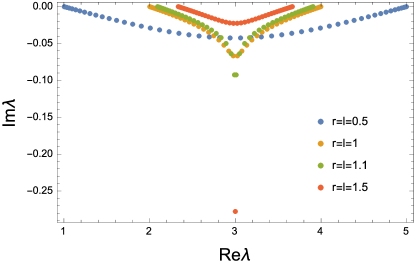
Fig. 2: (Color Online) The distribution of the eigenvalues $\lambda$ for $N=50,\epsilon=3,\Gamma_{L}=\Gamma_{R}=1$. The horizontal axis is the real part of the eigenvalue. We change the parameter $\gamma$ to satisfy $r=l=0.5,\ 1,\ 1.1,\ 1.5$. We can see that the special eigenvalues appear in $r=l>1$.

Fig. 4 shows the distribution of the eigenvalues for several numbers of the sites $N$. From this graph, the imaginary parts of the special eigenvalues do not disappear and do not change their values even in the large $N$ limit. In contrast, the imaginary parts of other eigenvalues decrease as the number of the sites $N$ increases shown in Fig. 4. Fig. 4 is the graph of the distribution of the normal eigenvalues for several $N$. The imaginary parts of the normal eigenvalues gradually decrease with $O(1/N)$ as the number of the sites increases[17].

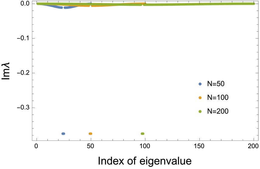
Fig. 3: (Color Online) The distribution of the imaginary parts of the eigenvalues for $\epsilon=3,\Gamma_{L}=\Gamma_{R}=1,\gamma=0.25$ as a function of the label of the eigenvalue. We consider the cases: $N=50,100,200$. For all numbers of sites, the imaginary part of the special eigenvalue takes the same value.

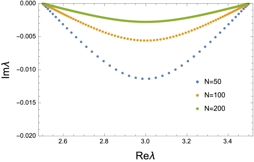
Fig. 4: (Color Online) The distribution of the imaginary parts of the normal eigenvalues for $\epsilon=3,\Gamma_{L}=\Gamma_{R}=1,\gamma=0.25$. We consider the cases: $N=50,100,200$. We can see that imaginary parts of the normal eigenvalues decrease as $O(\frac{1}{N})$.

Until now, we study the eigenvalues in limit $N\rightarrow\infty$. Next we consider the case of finite $N$, where we show a symmetry of the distribution of the eigenvalues for analysis of the electron density in the steady state and see an expression of the eigenvectors. First we obtain another expression of the characteristic equation (6). We express the LHS of Eq. (6) as $\Delta_{N}(\tilde{\lambda})$. By using the identity $\beta^{N}-\alpha^{N}=(\beta+\alpha)(\beta^{N-1}-\alpha^{N-1})-\alpha\beta(\beta^{N-2}-\alpha^{N-2})$, we can show that $\Delta_{N}(\tilde{\lambda})$ satisfies the following recurrence relation

$$\Delta_{N}(\tilde{\lambda})=\tilde{\lambda}\Delta_{N-1}(\tilde{\lambda})-\Delta_{N-2}(\tilde{\lambda}),$$ (9)

for $N\geq 2$ with the initial conditions $\Delta_{0}(\tilde{\lambda})=lr+1$ and $\Delta_{1}(\tilde{\lambda})=\tilde{\lambda}+i(l+r)$. For derivation, we use $\alpha\beta=1$ from (7). Polynomials which satisfy the recurrence relation (9) are called the modified Chebyshev polynomials[39]. It is known[39] that any modified Chebyshev polynomial $g_{N}(z)$, $z\in\mathbf{C}$ is expressed as

$$g_{N}(z)=g_{1}(z)V_{N-1}(z)-g_{0}(z)V_{N-2}(z),$$ (10)

where $V_{N}(z)=U_{N}(z/2)$ is the modified Chebyshev polynomial of the second kind and $U_{N}(\cos\Theta)=\sin((N+1)\Theta)/\sin(\Theta)$, $\Theta\in\mathcal{C}$, is the Chebyshev polynomial of the first kind. Using this property in our case $g_{N}=\Delta_{N}$, we obtain the expression $\Delta_{N}(\tilde{\lambda})=(\tilde{\lambda}+i(l+r))V_{N-1}(\tilde{\lambda})-(lr+1)V_{N-2}(\tilde{\lambda})$. By changing the variable $\tilde{\lambda}=2\cos\Theta$, we finally arrive at another expression for the characteristic equation[40]

$$(2\mathrm{cos}\Theta+i(l+r))\mathrm{sin}N\Theta-(lr+1)\mathrm{sin}(N-1)\Theta=0,$$ (11)

$$\tilde{\lambda}=2\mathrm{cos}\Theta.$$

Eq. (11) has all the information about the eigenvalues. From this expression, we can show a symmetry about the distribution of the eigenvalues $\tilde{\lambda}_{k}$. When Eq. (11) has a solution $\tilde{\lambda}_{k}$, there is the corresponding eigenvalue $-(\tilde{\lambda}_{k})^{*}$, which we call the conjugate eigenvalue of $\tilde{\lambda}_{k}$. We can prove this as follows. By dividing Eq. (11) by $\sin\Theta$ and applying the recurrence relation $2\tilde{\lambda}U_{N}(\tilde{\lambda})-U_{N-1}(\tilde{\lambda})=U_{N+1}(\tilde{\lambda})$, we have the expression,

$$U_{N+1}(\tilde{\lambda}_{k})+i(l+r)U_{N}(\tilde{\lambda}_{k})-lrU_{N-1}(\tilde{\lambda}_{k})=0.$$ (12)

This expression can also be derived from Eq. (7) by setting $\alpha=e^{i\Theta_{k}}$. By taking the complex conjugate of Eq. (12), we have

$$(U_{N+1}(\tilde{\lambda}_{k})+i(l+r)U_{N}(\tilde{\lambda}_{k})-lrU_{N-1}(\tilde{\lambda}_{k}))^{*} =U_{N+1}(\tilde{\lambda}^{*}_{k})-i(l+r)U_{N}(\tilde{\lambda}^{*}_{k})-lrU_{N-1}(\tilde{\lambda}^{*}_{k})$$

$$=(-1)^{N+1}U_{N+1}(-\tilde{\lambda}^{*}_{k})-(-1)^{N}i(l+r)U_{N}(-\tilde{\lambda}^{*}_{k})$$

$$\qquad-lr(-1)^{N-1}U_{N-1}(-\tilde{\lambda}^{*}_{k})$$

$$=U_{N+1}(-\tilde{\lambda}^{*}_{k})+i(l+r)U_{N}(-\tilde{\lambda}^{*}_{k})-lrU_{N-1}(-\tilde{\lambda}^{*}_{k})$$

$$=0.$$

From the first line to the second line, we use the relation about the Chebyshev polynomial of the second kind $U_{N}(-z)=(-1)^{N}U_{N}(z)$. This result shows that $-(\tilde{\lambda}_{k})^{*}$ is also the eigenvalue when $\tilde{\lambda}_{k}$ is the eigenvalue. We can see this from Fig. 2. Except for the case where $\lambda_{k}$ is a pure imaginary number, there is always the conjugate eigenvalue $-(\tilde{\lambda}_{k})^{*}$ of the eigenvalue $\lambda_{k}$.

Finally we discuss the eigenvector $\mathbf{r}_{k}$ corresponding to the eigenvalue $\lambda_{k}$. Because of the fact $(\mathbf{h}^{eff})^{t}=\mathbf{h}^{eff}$, the following relation about the eigenvectors holds

$$\sum_{k}\frac{\mathbf{r}_{k}\mathbf{r}^{t}_{k}}{\mathbf{r}^{t}_{k}\cdot\mathbf{r}_{k}}=\sum_{k}\mathbf{R}_{k}=1,$$ (13)

where we define $\mathbf{R}_{k}=\frac{\mathbf{r}_{k}\mathbf{r}^{t}_{k}}{\mathbf{r}^{t}_{k}\cdot\mathbf{r}_{k}}$. The concrete expression for the eigenvector is written as[40]

$$\mathbf{r}^{(n)}_{k}=\sin n\Theta_{k}+il\sin(n-1)\Theta_{k}.$$ (14)

Especially, the eigenvector $\mathbf{r}_{\Lambda_{l}}$ for the special eigenvalue, $\Lambda_{l}$, is written as

$$\mathbf{r}^{(n)}_{\Lambda_{l}}=-\frac{(-il)^{-n+1}}{2}(l+\frac{1}{l}).$$ (15)

From these expression above, $[\mathbf{R}_{k}]_{nm}$ and $[\mathbf{R}_{\Lambda_{l}}]_{nm}$, which is $\mathbf{R}_{k}$ of the special eigenvalue $\Lambda_{l}$, are expressed as

$$[\mathbf{R}_{k}]_{nm}\eqsim\frac{2}{N}\frac{(\sin n\Theta_{k}+il\sin(n-1)\Theta_{k})(\sin m\Theta_{k}+il\sin(m-1)\Theta_{k})}{1-l^{2}+2il\cos\Theta_{k}},$$ (16)

$$[\mathbf{R}_{\Lambda_{l}}]_{nm}\eqsim-(1+l^{2})(-il)^{-(n+m)}.$$ (17)

We prove Eq. (15) to Eq. (17) in Appendix A. Here $\eqsim$ means that we ignore the order of $O(1/N)$. The symmetry of the eigenvalues is written in terms of the eigenvectors as follows. Since we can express the conjugate eigenvalue as $-(\tilde{\lambda}_{k})^{*}=-2\cos(\Theta_{k})^{*}=2\cos(\Theta^{*}_{k}+\pi)$, we can obtain the corresponding eigenvector of the conjugate eigenvalue by adding $\pi$ to the phase $\Theta^{*}_{k}$ in the eigenvector (14). The result is

$$\sin j(\Theta^{*}_{k}+\pi)+il\sin(j-1)(\Theta^{*}_{k}+\pi) =(-1)^{j}(\sin j\Theta^{*}_{k}-il\sin(j-1)\Theta^{*}_{k})$$

$$=(-1)^{j}(\mathbf{r}^{j}_{k})^{*}.$$ (18)

We use this relation to study the electron density in the steady state.

4 Steady state

In this and the next section, we investigate the behavior of the electron density in our open system. First we consider the case of steady state and investigate boundary effects, especially the effects of the special eigenvalues, to the electron density. To carry out it, we derive a simple expression for the electron density in the steady state for general number of site $N$ and absolute zero temperature case $\beta=\infty$. We need this manipulation because we do not have an concrete expression of the eigenvalues themselves for general $N$ as we see in the previous section and therefore cannot know the qualitative behavior of the electron density in the steady state from the original representation (20). From the simple expression of the electron density in the steady state, first we show that a phase transition, whose behavior is the same as that obtained in the isolated case[38], also exists in our open case. In addition, we can analytically derive $\rho^{ss}_{n}=\frac{1}{2}$ for $\epsilon=V=0$ with the expression and the symmetric distribution of the eigenvalues. These behavior has been seen in the analysis of QME[4, 11], but the formulation is different from our model. About effects of the special eigenvalues, we confirm that the special eigenvalues do not change the qualitative behavior of the electron density in the steady state for thermodynamic limit $N\rightarrow\infty$.

From the expression for the time-dependent electron density (2), we can obtain the expression for the electron density in the steady state $\rho^{ss}$ as

$$\mathbf{\rho}^{ss}=\int^{\infty}_{-\infty}\frac{d\omega}{2\pi}\sum_{\alpha}f(\omega)\mathbf{\Lambda}_{\alpha}(\omega+V_{\alpha}),$$ (19)

whose $n$th diagonal element expresses the electron density at site $n$. This is because the second and the third term in (2) have the term $e^{-i\mathbf{h}^{eff}(t-t_{0})}$ which vanishes in the limit $t\rightarrow\infty$ as the imaginary parts of the eigenvalues of $\mathbf{h}^{eff}$ are negative. To know the behavior of the electron density (19) in detail, we rewrite the expression (19) using the eigenvalues $\lambda_{k}$ and the eigenvectors $\mathbf{r}_{k}$ of $\mathbf{h}^{eff}$. By using the relation (13), we have the following expression

$$\mathbf{\rho}^{ss} =\sum_{\alpha}\sum_{k,l}\left[\mathbf{R}_{k}\mathbf{\Gamma}_{\alpha}\mathbf{R}^{*}_{l}\right]\int^{\infty}_{-\infty}\frac{d\omega}{2\pi}f(\omega-\mu)\frac{1}{(\omega+V_{\alpha}-\lambda_{k})(\omega+V_{\alpha}-\lambda^{*}_{l})}$$

$$=\sum_{\alpha}\sum_{k,l}\left[\mathbf{R}_{k}\mathbf{\Gamma}_{\alpha}\mathbf{R}^{*}_{l}\right]\frac{1}{\lambda_{k}-\lambda^{*}_{l}}\left(F_{1}(\lambda_{k}-V_{\alpha})-F_{1}(\lambda^{*}_{l}-V_{\alpha})\right),$$ (20)

where we define $F_{1}(\lambda)=\int^{\infty}_{-\infty}\frac{d\omega}{2\pi}f(\omega-\mu)\frac{1}{\omega-\lambda}$. We note that all the effects of temperature $\beta$ are included in $F_{1}(\lambda)$. In the case of $\beta=\infty$, we can write the analytical expression for $F_{1}(\lambda)$ in (20) as

$$F_{1}(\lambda_{k}-V_{\alpha})-F_{1}(\lambda^{*}_{l}-V_{\alpha}) =\frac{1}{2\pi}\left[\log(\omega-(\lambda_{k}-V_{\alpha}))-\log(\omega-(\lambda^{*}_{l}-V_{\alpha}))\right]^{0}_{-\infty}$$

$$=\frac{1}{2\pi}(\log(V_{\alpha}-\lambda_{k})-\log(V_{\alpha}-\lambda^{*}_{l})-2\pi i),$$ (21)

where we use the fact $\mathrm{Im}(\lambda_{k})<0$. By substituting the expression (21) into (20), we have

$$\mathbf{\rho}^{ss} =\frac{1}{2\pi}\sum_{\alpha}\sum_{k,l}\left[\mathbf{R}_{k}\mathbf{\Gamma}_{\alpha}\left(\mathbf{R}_{l}\right)^{*}\right]\frac{1}{\lambda_{k}-\lambda^{*}_{l}}(\log(V_{\alpha}-\lambda_{k})-\log(V_{\alpha}-\lambda^{*}_{l})-2\pi i)$$

$$=1+\frac{1}{2\pi}\sum_{\alpha}\sum_{k,l}\left[\mathbf{R}_{k}\mathbf{\Gamma}_{\alpha}\left(\mathbf{R}_{l}\right)^{*}\right]\frac{1}{\lambda_{k}-\lambda^{*}_{l}}(\log(V_{\alpha}-\lambda_{k})-\log(V_{\alpha}-\lambda^{*}_{l})),$$ (22)

where we use the fact $-i\sum_{k,l}\mathbf{R}_{k}\mathbf{\Gamma}\mathbf{R}^{*}_{l}/(\lambda_{k}-\lambda^{*}_{l})=\mathbf{1}$ proved in Appendix B. We change the expression (22) into the more convenient form to discuss the behavior of the electron density in the steady state. By rearranging the expression (22) as in Appendix B, we have the following representation for any $V_{L}$ and $V_{R}$

$$\mathbf{\rho}^{ss} =1+\frac{i}{2\pi}\sum_{\alpha}(\log(V_{\alpha}-\mathbf{h}^{eff})-\log(V_{\alpha}-(\mathbf{h}^{eff})^{*}))$$

$$\quad-\frac{1}{2\pi}\sum_{k,l}\mathbf{R}_{k}\frac{1}{\lambda_{k}-\lambda^{*}_{l}}\bigl{(}(\log(V_{L}-\lambda_{k})-\log(V_{L}-\lambda^{*}_{l}))\mathbf{\Gamma}_{R}$$

$$\qquad+(\log(V_{R}-\lambda_{k})-\log(V_{R}-\lambda^{*}_{l}))\mathbf{\Gamma}_{L}\bigr{)}\left(\mathbf{R}_{l}\right)^{*}.$$ (23)

In addition, we assume symmetric bias voltages $V_{L}=V_{R}=V$ for simplicity. From the assumption, the electron density (23) is written as

$$\mathbf{\rho}^{ss} =1+\frac{i}{\pi}(\log(V-\mathbf{h}^{eff})-\log(V-(\mathbf{h}^{eff})^{*}))$$

$$\quad-\frac{1}{2\pi}\sum_{k,l}\mathbf{R}_{k}\mathbf{\Gamma}\left(\mathbf{R}_{l}\right)^{*}\frac{1}{\lambda_{k}-\lambda^{*}_{l}}\bigl{(}\log(V-\lambda_{k})-\log(V-\lambda^{*}_{l})\bigr{)}$$

$$=1+\frac{i}{\pi}(\log(V-\mathbf{h}^{eff})-\log(V-(\mathbf{h}^{eff})^{*}))-(\rho^{ss}-1),$$ (24)

where we use the definition of $\rho^{ss}$, (22) to obtain the final line. Therefore, the electron density takes the simple form

$$\mathbf{\rho}^{ss} =1+\frac{i}{2\pi}(\log(V-\mathbf{h}^{eff})-\log(V-(\mathbf{h}^{eff})^{*}))$$

$$=1+\frac{i}{2\pi}(\sum_{k}\mathbf{R}_{k}\log(V-\lambda_{k})-\mathbf{R}^{*}_{k}\log(V-\lambda^{*}_{k}))$$

$$=1-\frac{1}{\pi}\mathrm{Im}\left[\sum_{k}\mathbf{R}_{k}\log(V-\lambda_{k})\right]$$

$$=1-\frac{1}{\pi}\mathrm{Im}\left[\log(V-\mathbf{h}^{eff})\right].$$ (25)

With the expression (25), we discuss the behavior of the electron density in the steady state for the case $N\rightarrow\infty$. Without loss of generality, we set $V=0$ in the discussion since $V$ is just a shift of the energy.

First we investigate the average electron density per site $\bar{\rho}=\frac{1}{N}\mathrm{Tr}\mathbf{\rho}^{ss}$. By taking the trace of Eq.(25) and dividing by $N$, we have the following expression

$$\bar{\rho} =1-\frac{1}{N}\frac{1}{\pi}\mathrm{Im}\left[\mathrm{Tr}\log(-\mathbf{h}^{eff})\right]$$

$$=1-\frac{1}{N}\frac{1}{\pi}\mathrm{Im}\left[\log(\mathrm{det}(-\mathbf{h}^{eff}))\right]$$

$$=1-\frac{1}{N}\frac{1}{\pi}\mathrm{Im}\left[\log(\prod_{k}(-\lambda_{k}))\right]$$

$$=1-\frac{1}{N}\frac{1}{\pi}\sum_{k}\mathrm{arg}(-\lambda_{k}).$$ (26)

From the first to the second line, we use $\mathrm{Tr}\log(-\mathbf{h}^{eff})=\log\mathrm{det}(-\mathbf{h}^{eff})$. From this expression, we can show that a phase transition exits in our open system as follows. First we consider the case $r,l<1$ for simple discussion, where there is no special eigenvalue. We discuss the case with special eigenvalues later. In the following discussion, we use the fact that the eigenvalues are expressed as $\lambda_{k}\eqsim\epsilon+2\gamma\cos k+i0$, $k\in(0,\pi)$ for large $N$ as we show in Section 3. $\eqsim$ means that we ignore the terms of order $O(1/N)$. With this fact and the expression (26), we can see that there are three situations depending on the parameter $\epsilon$ and $\gamma$. See the Fig. 5.

Fig. 5: (Color Online) Distribution of $-\lambda_{k}$ for large $N$. For the case $\epsilon>2\gamma$(solid line), all the eigenvalues are on the negative real line, whose argument are $\pi$. In contrast, the argument of all eigenvalues are $0$ for the case $\epsilon<-2\gamma$ since they are on the positive real line(dots line). When $-2\gamma<\epsilon<2\gamma$ is satisfied, some eigenvalues are on the negative real line and the others are on the positive real line(dashed line).

In the case $\epsilon>2\gamma$, $-\lambda_{k}$ are always on the negative real line. Therefore, $\mathrm{arg}(-\lambda_{k})=\pi$ holds and the average electron density per site is $\bar{\rho}=0$ from (26). When $-2\gamma<\epsilon<2\gamma$ is satisfied, we set $N^{*}$ as the number of eigenvalues which satisfy $\epsilon+2\gamma\cos k<0$. Then the average electron density is expressed as $\bar{\rho}=1-N^{*}/N$. In the limit $N\rightarrow\infty$, we can easily prove the behavior is arccosine from Eq. (26) and the result is compatible with the numerical result (Fig. 6). For the case of $\epsilon<-2\gamma$, all the eigenvalues are on the positive real line and the argument $\mathrm{arg}(-\lambda_{k})$ is 0. Therefore, the average electron density is $\bar{\rho}=1$. In this way, we can see that the phase transition exits in the open case at $\left|\frac{\epsilon}{2\gamma}\right|=1$ and the behavior is the same result obtained in the isolated case[38]. Actually, we can numerically show the phase transition as in Fig. 6 obtained by computing the definition of the electron density in the steady state (20).

Fig. 6: (Color Online) The average electron denisty $\bar{\rho}$ and the on-site energy $\epsilon$. The parameters are set as $N=50,\ V_{L}=V_{R}=0,\ \Gamma_{L}=\Gamma_{R}=\gamma=0.5$. The average electron density discontinuously changes at $\left|\frac{\epsilon}{2\gamma}\right|=1$.

We can physically understand this behavior as follows. When the on-site energy $\epsilon$ is too high, which corresponds to the case of $\epsilon>2\gamma$, all electrons outflow from the sites to the reservoirs and the average density finally becomes 0 in the steady state. In contrast, electrons are accumulated until the sites are filled with electrons for the case of $\epsilon>-2\gamma$. Therefore, the average electron density is 1 in the steady state. When the same bias voltages $V$ are applied to the reservoirs, the effect is just shifting the graph in Fig. 6 along the horizontal line. Next we consider the effect of the special eigenvalues to the behavior of the average electron density. Actually, the special eigenvalue does not affect the average electron density in the limit $N\rightarrow\infty$. We can understand this as follows. Let us consider the case $l<1,r>1$ where there is one special eigenvalues $\Lambda_{r}$. In this case, the average electron density (26) for large $N$ is written as

$$\bar{\rho}=1-\frac{1}{N}\frac{1}{\pi}\left(\sum_{k:\mathrm{normal}}\mathrm{arg}(-\lambda_{k})+\mathrm{arg}(-\Lambda_{r})\right).$$ (27)

From the Eq. (27), we can see that the term from the special eigenvalue vanishes in the $N\rightarrow\infty$ since the order of $\mathrm{arg}(-\Lambda_{r})$ is $O(N^{0})$. Therefore, the average electron density with the special eigenvalue in $N\rightarrow\infty$ behaves in a similar way as the case without special eigenvalue.

We also discuss the electron density at each site. First we analytically prove that the electron density at any site takes the same value $\rho^{ss}_{n}=\frac{1}{2}$ for the case $\epsilon=V=0$. A similar situation is considered with the different approach of QME[11] and the result is the same. After that, we numerically investigate the dependence of the electron density at each site on the boundary parameters. As a result, we see that the qualitative behavior of the electron density in the steady state does not change by the special eigenvalues. For simplicity, we consider the case where the number of the sites is even $N=2M$. In the case $\epsilon=0$, the eigenvalue is expressed for $\lambda_{k}=\gamma\tilde{\lambda}_{k}$ from the definition (7). From the Eq. (25), we have

$$\rho^{ss}_{n} =1-\frac{1}{\pi}\mathrm{Im}\sum^{N}_{k=1}\left[\mathbf{R}_{k}\right]_{nn}\log(-\lambda_{k})$$

$$=1-\frac{1}{\pi}\mathrm{Im}\sum^{M}_{k=1}\left[[\mathbf{R}_{k}]_{nn}\log(-\gamma\tilde{\lambda}_{k})+[\mathbf{R}^{*}_{k}]_{jj}\log(\gamma\tilde{\lambda}^{*}_{k})\right],$$

where we use the symmetric distribution of the normalized eigenvalue, which means that there are always the corresponding eigenvalue $-\tilde{\lambda}^{*}_{k}$ and the matrix $(-1)^{n+m}[\mathbf{R}^{*}_{k}]_{nm}$ to the eigenvalue $\tilde{\lambda}_{k}$ and the matrix $[\mathbf{R}_{k}]_{nm}$. We can prove this fact from (18). With the relations $|\gamma\tilde{\lambda}^{*}_{k}|=|-\gamma\tilde{\lambda}_{k}|$ and $\mathrm{arg}(-\gamma\tilde{\lambda}_{k})=\pi-\mathrm{arg}(\gamma\tilde{\lambda}^{*}_{k})$, we can express $\rho^{ss}_{n}$ as

$$\rho^{ss}_{n} =1-\frac{1}{\pi}\mathrm{Im}\sum^{M}_{k=1}\bigg{[}[\mathbf{R}_{k}]_{nn}(\log|-\gamma\tilde{\lambda}_{k}|+i\mathrm{arg}(-\gamma\tilde{\lambda}_{k}))+[\mathbf{R}^{*}_{k}]_{nn}(\log|-\gamma\tilde{\lambda}_{k}|+i(\pi-\mathrm{arg}(-\gamma\tilde{\lambda}_{k}))\bigg{]}$$

$$=1-\mathrm{Im}\sum^{M}_{k=1}i[\mathbf{R}^{*}_{k}]_{nn}$$

$$=1-\mathrm{Re}\sum^{M}_{k=1}[\mathbf{R}^{*}_{k}]_{nn}.$$

Again we use the fact of the symmetric distribution of the normalized eigenvalue and the eigenvector. Finally, we can write the electron density $\rho^{ss}_{n}$ for $\epsilon=0$ as

$$\rho^{ss}_{n} =1-\frac{1}{2}\sum^{M}_{k=1}[\mathbf{R}_{k}]_{nn}+[\mathbf{R}^{*}_{k}]_{nn}$$

$$=1-\frac{1}{2}\sum^{N}_{k=1}[\mathbf{R}_{k}]_{nn}$$

$$=\frac{1}{2}.$$ (28)

To obtain the final result, we use Eq. (13).

Fig. 7: (Color Online) The electron denisty $\rho_{n}$ for several $\epsilon$. The parameters are set as $N=30,\ V_{L}=V_{R}=0,\ \Gamma_{L}=\Gamma_{R}=\gamma=0.5$. The electron density at each site discontinuously changes at $\epsilon=2\gamma=1$

Fig. 8: (Color Online) The electron denisty $\rho_{n}$ for $-2\gamma<\epsilon<2\gamma$. The parameters are set as $N=30,\ V_{L}=V_{R}=0,\ \Gamma_{L}=\Gamma_{R}=\gamma=0.5$. In this region, the electron density at each site fluctuates.

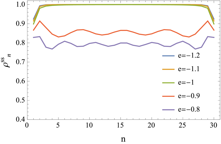
Fig. 9: (Color Online) The electron denisty $\rho_{n}$ for several $\epsilon$. The parameters are set as $N=30,\ V_{L}=V_{R}=0,\ \Gamma_{L}=\Gamma_{R}=\gamma=0.5$. The electron density at each site discontinuously changes at $\epsilon=-2\gamma=-1$

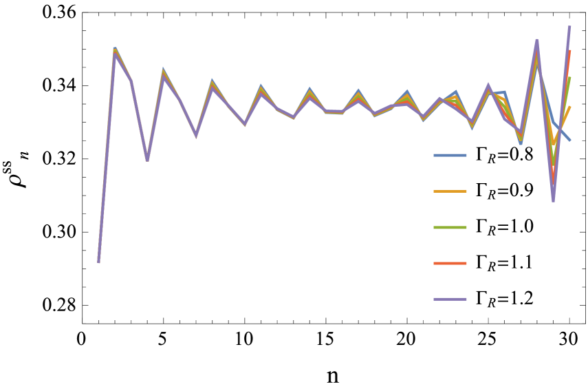
Fig. 10: (Color Online) The electron denisty $\rho_{n}$ for several $\Gamma_{R}$. The parameters are set as $N=30,\ V_{L}=V_{R}=0,\ ,\epsilon=\Gamma_{L}=\gamma=0.5$. We cannot see any discontinuous behavior at $r=\frac{\Gamma_{R}}{2\gamma}=1$.

We numerically calculate the electron density at site $n$ in the steady state from the definition (20) for several energy $\epsilon$. The results are Fig. 8, Fig. 8 and Fig. 10. These figures show that the phase transition at $|\frac{\epsilon}{2\gamma}|=1$ also exists not only in the average electron density but also in the electron density at each site except the sites on the edges. We call the sites not the left most site and the right most site as the bulk sites for explanation. From Fig. 8, we can see that the electron density is almost 0 on the bulk sites for the case $\epsilon>2\gamma$. When the parameters satisfy $\epsilon<-2\gamma$, the electron density on the bulk sites are almost 1 as Fig. 10 shows. The value of the electron density suddenly changes at $\epsilon=2\gamma$ and $\epsilon=-2\gamma$. The behavior is the same as that of the average electron density. For the case where $-2\gamma<\epsilon<2\gamma$, there is a difference from the average electron density(Fig. 8). The electron density fluctuates by sites around the average electron density except $\epsilon=0$. At $\epsilon=0$, the electron density does not depend on the site index and it takes the same value $\rho^{ss}_{n}=\frac{1}{2}$, which we have shown analytically (28). The fluctuation is suppressed as the on-site energy $\epsilon$ is close to $0$. We also study the dependence of $\rho^{ss}_{n}$ on the coupling parameter at the right boundary $\Gamma_{R}$ to see the effect of the special eigenvalue(Fig. 10). In the settings, the special eigenvalue appears at $\Gamma_{L}=1$. However, we cannot see any discontinuous behavior at $r=1$ from Fig. 10. In conclusion, the phase transition of the electron density in the steady state, whose behavior is the same as that of the isolated tight-binding model, also exists in our open case. The boundary terms do not break the phase transition and do not change the qualitative behavior of the electron density by the special eigenvalue.

5 Time-dependent case

Next we consider the time-dependent case, which is of our main interest and investigate the effect of the boundary parameters. With the calculation technique used also in the analysis of steady state, we derive an analytical expression of the time-dependent electron density for $N\rightarrow\infty$ and zero temperature case $\beta=\infty$. From the expression, first we see that a two-step relaxation appears in the time-dependent electron density caused by boundary couplings for the case of $\epsilon<V+2\gamma$, which cannot be seen in the previous study about the dynamics of isolated case[32]. Because of the boundary couplings, particles flow and the time lag between flow of particles from the left and the right reservoir causes the two-step decay, which we understand later using Fig. 13. For the case of $\epsilon\geq V+2\gamma$, the time-dependent electron density decays to 0 quickly. This is because the on-site energy of the dots are too high and electrons cannot remain in the dots. Next we study the effects of the special eigenvalues to the time-dependent electron density. By computing the analytical expression of the electron density for the case with special eigenvalues, we find that the dependence of speed of convergence to steady state on the boundary couplings changes by the special eigenvalue. We can expect that the speed of convergence increase as the couplings on the boundaries become large because the boundary couplings determine how easily particles from reservoirs can flow into the sites. However, the dependence changes by the special eigenvalues at $l=1$ and $r=1$ and the speed decrease as the couplings become large. We check this fact from numerical calculation of the definition of the time-dependent electron density (Fig. 17).

We start our analysis from the formal expression of the electron density (2). The time-dependent part of the electron density is expressed as

$$\rho(t)-\rho^{ss} =\sum_{\alpha=\{L,R\}}\int^{\infty}_{-\infty}\frac{d\omega}{2\pi}f(\omega-\mu)V_{\alpha}(e^{-i\mathbf{h}^{eff}(t-t_{0})}\mathbf{G}^{r}(\omega)\mathbf{\Lambda}_{\alpha}(\omega+V_{\alpha})e^{i(\omega+V_{\alpha})(t-t_{0})}+\mathrm{H.c.})$$

$$\quad+V^{2}_{\alpha}e^{-i\mathbf{h}^{eff}(t-t_{0})}\mathbf{G}^{r}(\omega)\mathbf{\Lambda}_{\alpha}(\omega+V_{\alpha})\mathbf{G}^{a}(\omega)e^{i(\mathbf{h}^{eff})^{*}(t-t_{0})}$$

$$=\sum_{\alpha=\{L,R\}}2\mathrm{Re}[\mathbf{\rho}^{(1)}_{\alpha}(t)]+\mathbf{\rho}^{(2)}_{\alpha}(t).$$ (29)

First we investigate the behavior of $\mathbf{\rho}^{(1)}_{\alpha}(t)$. This is because $\mathbf{\rho}^{(2)}_{\alpha}(t)$ behaves in almost the same manner as $\mathbf{\rho}^{(1)}_{\alpha}(t)$ as we see later. For simplicity, we assume a symmetric and large bias voltages: $V_{L}=V_{R}=V$ and $V\gg|\lambda_{k}-\lambda^{*}_{l}|\eqsim 4\gamma$. We study other cases using numerical calculation. By using the assumption of the symmetric bias voltages and carrying out the same calculation as in the derivation of (23), we have the following expression

$$\mathbf{\rho}^{(1)}(t) =\sum_{\alpha=\{L,R\}}\mathbf{\rho}^{(1)}_{\alpha}(t)$$

$$=i\sum_{k}\mathbf{R}_{k}e^{-i(\lambda_{k}-V)t}(F_{2}(t,\lambda_{k})-F_{2}(t,\lambda_{k}-V))$$

$$\quad-i\sum_{k,l}\mathbf{R}_{k}\mathbf{R}^{*}_{l}\frac{V}{\lambda_{k}-\lambda^{*}_{l}+V}e^{-i(\lambda_{k}-V)t}(F_{2}(t,\lambda_{k})-F_{2}(t,\lambda^{*}_{l}-V)),$$ (30)

where we define $F_{2}(t,z)=\int^{\infty}_{-\infty}\frac{d\omega}{2\pi}f(\omega-\mu)\frac{e^{i\omega t}}{\omega-z}$. $F_{2}(t,z)$ includes all the effects of the temperature. We can express $F_{2}(t,z)$ for $\beta=\infty$ as

$$F_{2}(t,z)=\frac{e^{itz}}{2\pi}\times\begin{cases}\left(-E_{1}(itz)+2\pi i\right),&\mathrm{Re}z<0\ \mathrm{and}\ \mathrm{Im}z>0,\\ -E_{1}(itz),&\mathrm{else},\end{cases}$$ (31)

where $E_{n}(x)=z^{n-1}\int^{\infty}_{z}\frac{e^{-t}}{t^{n}}$ is the $n$th order of the exponential integral with its principal value. The derivation is in Appendix C. We note that $F_{2}(t,z)$ is a multivalued function. The two cases in the expression (31) arises due to the branch cut of the exponential function $E_{1}(z)$ on the negative real line. At this point, we use the assumption of the large bias voltages $V\gg 4\gamma$. From this assumption, the relation $\frac{V}{\lambda_{k}-\lambda^{*}_{l}+V}\eqsim 1$ holds, where we ignore the order of $O(\frac{1}{V})$. By using the relation, we can rewrite (30) in a simple form as

$$\mathbf{\rho}^{(1)}(t) =i\sum_{k}\mathbf{R}_{k}e^{-i(\lambda_{k}-V)t}(F_{2}(t,\lambda_{k})-F_{2}(t,\lambda_{k}-V))$$

$$\quad-i\sum_{k,l}\mathbf{R}_{k}\mathbf{R}^{*}_{l}e^{-i(\lambda_{k}-V)t}(F_{2}(t,\lambda_{k})-F_{2}(t,\lambda^{*}_{l}-V))$$

$$=-i\sum_{k}\mathbf{R}_{k}e^{-i(\lambda_{k}-V)t}F_{2}(t,\lambda_{k}-V)+i\sum_{k,l}\mathbf{R}_{k}\mathbf{R}^{*}_{l}e^{-i(\lambda_{k}-V)t}F_{2}(t,\lambda^{*}_{l}-V)$$

$$=\mathbf{\rho}^{(1,1)}(t)+\mathbf{\rho}^{(1,2)}(t),$$ (32)

where we define

$$\mathbf{\rho}^{(1,1)}(t)=-i\sum_{k}\mathbf{R}_{k}e^{-i(\lambda_{k}-V)t}F_{2}(t,\lambda_{k}-V),$$ (33)

$$\mathbf{\rho}^{(1,2)}(t)=i\sum_{k,l}\mathbf{R}_{k}\mathbf{R}^{*}_{l}e^{-i(\lambda_{k}-V)t}F_{2}(t,\lambda^{*}_{l}-V).$$ (34)

We investigate the behavior of (33) and (34) in detail. As we will see, both quantities take different forms depending on the existence of the special eigenvalues, $\Lambda_{l}$ and $\Lambda_{r}$. From this fact, the dependence of convergence speed on the boundary parameters $l,r$ changes at $l=1$ and $r=1$. We also note that the term $\mathbf{\rho}^{(1,2)}(t)$ shows two-step decay for the case of $\epsilon<V+2\gamma$ and $l>0$ or $r>0$. In other words, the quantity have quasi-steady state if the on-site energy is not large enough to satisfy $\epsilon<V+2\gamma$ and there is a coupling between the edge dots and the reservoirs. This is because the argument of $F(t,\lambda^{*}_{l}-V)$ in $\mathbf{\rho}^{(1,2)}(t)$ crosses the branch cut on the negative real line for the case $\epsilon<V+2\gamma$ and a phase term arises. $\mathbf{\rho}^{(1,1)}(t)$ does not have the behavior of two-step decay because the argument of $F(t,\lambda_{k}-V)$ never cross the branch cut. We check these facts below.

First we consider the case $0<l<1$, where there is no special eigenvalue. As we prove in Appendix C, for the case of $N\rightarrow\infty$, we can express the $n$th diagonal part of $\mathbf{\rho}^{(1,1)}(t)$ as

$$\mathbf{\rho}^{(1,1)}_{n}(t) =\frac{i}{2\pi}\frac{\gamma}{l}\int^{\infty}_{t}ds\frac{e^{i(\epsilon-V)s}}{s}\int^{\infty}_{s}due^{\gamma(l-\frac{1}{l})(u-s)}h_{nn}(u,l),$$ (35)

where the integrand is defined as

$$h_{nm}(s,l) =I_{n-m}(-2\gamma is)-I_{n+m}(-2\gamma is)-l^{2}(I_{n-m}(-2\gamma is)-I_{n+m-2}(-2\gamma is))$$

$$\qquad+i2l(I^{\prime}_{n-m}(-2\gamma is)-I_{n+m-1}(-2\gamma is)).$$

$I_{n}(s)$ is the modified Bessel function of order $n$[41]. In Fig. 12, we check the correctness of the expression (35) by comparing the behavior of (35) with the numerical result calculated from the definition (33). The figure shows that there is good agreement between the analytical and the numerical result.

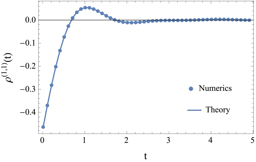
Fig. 11: (Color Online) The behavior of the quantity $\mathbf{\rho}^{(1,1)}_{1}(t)$ obtained numericaly(Blue dots) and analytically(Blue line). We set the parameters as $N=20,\ V_{L}=V_{R}=6,\ \epsilon=3,\ \Gamma_{R}=\gamma=0.5$. We can see the good agreement of the analytical result with the numerical result.

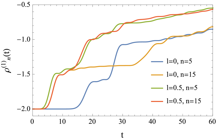
Fig. 12: (Color Online) The behavior of the quantity $\rho^{(1)}_{n}(t)$ by the site index $n$ and the coupling parameter $l$. We set the parameters as $N=20,\ V_{L}=V_{R}=6,\ \epsilon=3,\ \Gamma_{R}=\gamma=0.5$. We can see two-step decay.

In the similar way of deriving $\mathbf{\rho}^{(1,1)}(t)$, we can calculate $\mathbf{\rho}^{(1,2)}(t)$ for large $N$, whose expression changes according to the parameters $\epsilon$, $V$, and $\gamma$. For the case of $\epsilon>V+2\gamma$, which means that the on-site energy is large enough, $\mathbf{\rho}^{(1,2)}(t)$ is written as

$$\mathbf{\rho}^{(1,2)}_{n}(t)=-\frac{i}{2\pi}\sum^{N}_{m=1}A_{nm}(t)B_{mn}(t),$$ (36)

where $A_{nm}(t)$ and $B_{mn}(t)$ are expressed as

$$A_{nm}(t) =\sum_{k}[\mathbf{R}_{k}]_{nm}e^{-i\lambda_{k}t}$$

$$\xrightarrow{N\rightarrow\infty}\frac{\gamma}{l}e^{-i\epsilon t}\int^{\infty}_{t}dse^{\gamma(l-\frac{1}{l})(s-t)}h_{nm}(s,l),$$ (37)

$$B_{mn}(t) =\sum_{l}[\mathbf{R}^{*}_{l}]_{mn}e^{i\lambda^{*}_{l}t}E_{1}(it(\lambda^{*}_{l}-V))$$

$$\xrightarrow{N\rightarrow\infty}\frac{\gamma}{l}e^{i\epsilon t}\int^{\infty}_{t}ds\frac{e^{-i(\epsilon-V)}s}{s}\int^{s}_{-\infty}due^{-\gamma(l-\frac{1}{l})(u-s)}h^{*}_{mn}(u-t,l).$$ (38)

A short derivation of the expressions (37) and (38) is in Appendix C. Next we consider the case of $\epsilon<V+2\gamma$. In this situation, a phase term arises from $E_{1}(it(\lambda^{*}_{l}-V))$ in the definition of $B_{mn}(t)$, (38). To understand this fact, let us consider the distribution of the eigenvalues $\lambda^{*}_{k}-V$, which we can obtain from Fig. 5, the distribution of eigenvalues $-\lambda_{k}$, by folding its real value with respect to the imaginary axis and shifting $-V$ along the real axis. In this case $\epsilon<V+2\gamma$, the real parts of several eigenvalues $\mathrm{Re}(\lambda^{*}_{k}-V)\eqsim\epsilon+2\gamma\cos k-V$ are negative. By considering the fact that multiplying the imaginary number $i$ means rotating 90 degrees around the origin of the complex plane, the eigenvalues which satisfy $\mathrm{Re}(\lambda^{*}_{k}-V)<0$, cross the branch cut of $E_{1}(i(\lambda^{*}_{k}-V))$ on the negative real line. This leads to the appearance of the phase factor $2\pi i$ for several terms in the summation of $l$ (36). In the following, we consider the case $\epsilon<V-2\gamma$ for simple calculation. In the case of $\epsilon<V-2\gamma$, all the arguments in $E_{1}(it(\lambda^{*}_{l}-V))$ cross the branch cut. Therefore, $\mathbf{\rho}^{(1,2)}_{n}(t)$ changes from (37) to

$$\mathbf{\rho}^{(1,2)}_{n}(t)=-\frac{i}{2\pi}\sum^{N}_{m=1}(A_{nm}(t)B_{mn}(t)-2\pi i|A_{nm}(t)|^{2}).$$ (39)

We discuss the behavior of $\mathbf{\rho}^{(1,2)}_{n}(t)$ for $V-2\gamma<\epsilon<V+2\gamma$ later in Fig. 15. The second term in (39), $\sum_{m}|A_{nm}(t)|^{2}$, causes two-step decay. First we check this fact by numerically calculating the definition of $\rho^{(1)}(t)$ and analytically understand it later. We compute $\rho^{(1)}(t)$ instead of $\rho^{(1,2)}(t)$ because $\rho^{(1,1)}(t)$ converges to 0 very fast as Fig. 12 shows. The result is Fig. 12. We numerically calculate $\rho^{(1)}_{n}(t)$ from the definition (32) by diagonalizing the non-hermitian matrix for several combinations of the left coupling strength $0\leq l<1$ and site index $n$. We set the parameters as $N=20,\ V_{L}=V_{R}=6,\ \epsilon=3,\ \Gamma_{R}=\gamma=0.5$. From the graph, we can see the following. For the case $l=0$, where there is no coupling between the left reservoir and site 1, $\rho^{(1)}_{n}(t)$ has two-step decay and the start time of each decay depends on the site index $n$. For example, first decay occurs around the time $t=20+1-5=16$ and the second starts around the time $t=20+1+5=26$ for the case $n=5$. In contrast, for the case $n=15$, first decay occurs about the time $t=20+1-15=6$ and the second occurs about the time $t=20+1+15=36$. Therefore, we can expect that the start times change with the site index $n$. For the case of $l\neq 0$, however, the start times of the two-step decay are the same, $t=5$ and $t=15+1=16$, for both cases $n=5$ and $n=15$. In the following, we analytically understand these facts above. First we consider the case $l=0$, where we can simply express $|A_{nm}(t)|^{2}$ as

$$|A_{nm}(t)|^{2} =|h_{nm}(t,0)|^{2}$$

$$=((-1)^{n}J_{m-n}(2\gamma t)-J_{m+n}(2\gamma t))^{2}.$$ (40)

$J_{n}(t)$ is the Bessel function of the first kind. To obtain the expression in the second line, we use the relation $I_{n}(t)=i^{-n}J_{n}(it)$. We derive (40) from the definition in the same way as (37). We can obtain the same result by taking the limit $l\rightarrow 0$ of (37) and replacing $\lim_{l\rightarrow 0}e^{-\frac{t}{r}}/l$ for $t>0$ as $\delta(t)$. This replacement is not mathematically true because $\int^{\infty}_{-\infty}dt\lim_{r\rightarrow 0}e^{-\frac{t}{l}}/l\neq 1$, however, we can obtain the same expression in a simpler way. With the relation about the product of Bessel function $\sum^{\infty}_{-\infty}J_{n}J_{n-k}=\delta_{0,k}$, we can calculate the sum of (40) as

$$\sum^{N}_{m=1}|A_{nm}(t)|^{2} =\sum^{\infty}_{m=1}|A_{nm}(t)|^{2}-\sum^{\infty}_{m=N+1}|A_{nm}(t)|^{2}$$

$$=1-\sum^{\infty}_{m=N+1}|A_{nm}(t)|^{2}$$

$$=1-\sum^{\infty}_{m=N+1}\left(J^{2}_{m-n}(2\gamma t)+J^{2}_{m+n}(2\gamma t)-2(-1)^{n}J_{m-n}(2\gamma t)J_{m+n}(2\gamma t)\right).$$ (41)

From this expression, we can see that the sum $\sum^{N}_{n=1}|A_{nm}(t)|^{2}$ has two-step decay. To understand this, we use the fact that the products of Bessel function $J^{2}_{n}(t)$ and $J_{m-n}(t)J_{m+n}(t)$ take values which are almost 0 until $t\eqsim n,\ m-n$ respectively. We prove this in Appendix C. We consider the lowest order of each term in (41): $J^{2}_{N+1-n}(2\gamma t)$, $J^{2}_{N+1+n}(2\gamma t)$, and $J_{N+1-n}(2\gamma t)J_{N+1+n}(2\gamma t)$. Before the time $t<t_{1}=\frac{N+1-n}{2\gamma}$, all of the three terms take 0. The first and the third term have non-zero value in $t_{1}\leq t<t_{2}=\frac{N+1+n}{2\gamma}$. Around the time $t=t_{2}$, the second term start to have non-zero value and all the terms have finite values after the time. From the discussion above, we can conclude that the two decays start at $t_{1}=\frac{N+1-n}{2\gamma}$ and $t_{2}=\frac{N+1+n}{2\gamma}$. This is in good agreement with the numerical results of $\gamma=0.5$ in Fig. 12. We can explain the fact above in more intuitive way using Fig. 13.

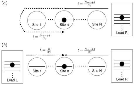
Fig. 13: Schematic diagram of transport for (a) $l=0,\ r\neq 0$ and (b) $l\neq 0,\ r\neq 0$. In the case $l=0$, Electrons from the left reservoir reach site $n$ around $t=\frac{N+1-n}{2\gamma}$(Real line) for the first time. After reflection at the right edge, the electrons come back to site $n$ around $t=\frac{N+1+n}{2\gamma}$(Dashed line). There are electrons from the right reservoir in the case $l\neq 0$, which comes to site $n$ around $t=n$(Dotted Line) or $t=\frac{N-n+1}{2\gamma}$(Real line).

We focus on the site $n$. Since the transport is ballistic, the time which a electron need to move $i$ sites linearly grows with the number $i$[32] with the normalization of $2\gamma$. Therefore, it takes time $t_{1}$ for an electron from the right reservoir in Fig. 13 $(a)$ to reach site $n$ and the electron density at site $n$ changes at the time $t_{1}$. After that, the electron is reflected at the left most dot around $t=N$. Then the electron density at site $n$ changes again at the time $t_{2}$ when the reflected electron comes back to the site $n$. This is the reason why the electron density changes at the times $t_{1}$ and $t_{2}$. With this understanding, we can study the case of $l>0$, Fig. 13 $(b)$. In this case, there are couplings between the reservoirs and both edges of the sites. Therefore, electrons are transported from the both reservoirs. At the time $t=\frac{n}{2\gamma}$ and $t=\frac{N-n+1}{2\gamma}$, the electrons from the reservoirs arrive at the site $n$ and the quantity changes $\rho^{(1)}_{n}(t)$. This is also compatible with the facts obtained from Fig. 12.

By carrying out a similar calculation as $\mathbf{\rho}^{(1)}(t)$, we can obtain an expression of $\mathbf{\rho}^{(2)}(t)$. From the expression, we can see that the behavior of $\mathbf{\rho}^{(2)}(t)$ is almost the same as $\mathbf{\rho}^{(1,2)}(t)$. Similar to the analysis of $\mathbf{\rho}^{(1)}(t)$, we consider a symmetric bias voltage $V_{L}=V_{R}=V$ and a large bias case $V\gg 4\gamma$ for simple calculation. In this case, we have the expression as

$$\mathbf{\rho}^{(2)}(t) =\sum_{\alpha=\{L,R\}}\mathbf{\rho}^{(2)}_{\alpha}(t)$$

$$=V^{2}\int^{\infty}_{-\infty}\frac{d\omega}{2\pi}f(\omega-\mu)\sum_{k,l}\mathbf{R}_{k}\mathbf{\Gamma}\mathbf{R}^{*}_{l}e^{-i(\lambda_{k}-\lambda^{*}_{l})t}\frac{1}{(\omega-\lambda_{k})(\omega+V-\lambda_{k})(\omega+V-\lambda^{*}_{l})(\omega-\lambda^{*}_{l})}$$

$$\eqsim\frac{1}{2\pi}\sum_{k,l}\mathbf{R}_{k}\mathbf{\Gamma}\mathbf{R}^{*}_{l}e^{-i(\lambda_{k}-\lambda^{*}_{l})t}\frac{1}{\lambda_{k}-\lambda^{*}_{l}}(F_{1}(\lambda_{k})-F_{1}(\lambda^{*}_{l})+F_{1}(\lambda_{k}-V)-F_{1}(\lambda^{*}_{l}-V)).$$ (42)

Details of the derivation are in Appendix C. We use the function $F_{1}(\lambda)$ defined in steady case again. For $\beta=\infty$, we can calculate $F_{1}(\lambda)$ of Eq. (42) in the same way as (21). The result is

$$\mathbf{\rho}^{(2)}(t) =\frac{1}{2\pi}\sum_{k,l}\mathbf{R}_{k}\mathbf{\Gamma}\mathbf{R}^{*}_{l}e^{-i(\lambda_{k}-\lambda^{*}_{l})t}\times$$

$$\qquad\frac{1}{\lambda_{k}-\lambda^{*}_{l}}(\log(-\lambda_{k})-\log(-\lambda^{*}_{l})+\log(V-\lambda_{k})-\log(V-\lambda^{*}_{l})-4\pi i),$$ (43)

For the case of large $N$ and $\epsilon>2\gamma$, we have the relation $\log(-\lambda_{k})-\log(-\lambda^{*}_{l})\eqsim 2\pi i$, which we can understand graphically from Fig. 5. Again $\eqsim$ means that we ignore the order of $O(1/N)$. In a similar way, the following relation holds

$$\log(V-\lambda_{k})-\log(V-\lambda^{*}_{l})\eqsim\begin{cases}0&\epsilon<V-2\gamma,\\ 2\pi i&\epsilon>V+2\gamma.\end{cases}$$

By substituting these relations into (43) and using $-i\sum_{k,l}\mathbf{R}_{k}\mathbf{\Gamma}\mathbf{R}^{*}_{l}/(\lambda_{k}-\lambda^{*}_{l})e^{-i(\lambda_{k}-\lambda^{*}_{l})t}=\sum_{k,l}\mathbf{R}_{k}\mathbf{R}^{*}_{l}/(\lambda_{k}-\lambda^{*}_{l})e^{-i(\lambda_{k}-\lambda^{*}_{l})t}$, which we can prove in a similar way as (B.1) in Appendix B, we have

$$\mathbf{\rho}^{(2)}_{n}(t)=\begin{cases}\sum^{N}_{m=1}|A_{nm}(t)|^{2}&\epsilon<V-2\gamma,\\ 0&\epsilon>V+2\gamma.\end{cases}$$ (44)

Details of the derivation is in Appendix C. Again, the same quantity $\sum^{N}_{m=1}|A_{nm}(t)|^{2}$ as in (39) appears. Therefore, the two-step decay also appears in $\mathbf{\rho}^{(2)}_{n}(t)$ in the similar way as $\mathbf{\rho}^{(1)}_{n}(t)$. By substituting (35), (36), and (5) into (29) with (32), we can obtain an analytical expression of the time-dependent part of the electron density. Based on the discussion above, we investigate the time-dependent part of the electron density itself for the case where there is no special eigenvalue with numerical calculation in Fig. 15 and Fig. 15. Below, we simply call the time-dependent part of the electron density as the time-dependent electron density because the effect of the steady-state value is just constant shifting. We confirm that the results obtained for the part of the electron density $\rho^{(1,2)}(t)$ also hold for the electron density.

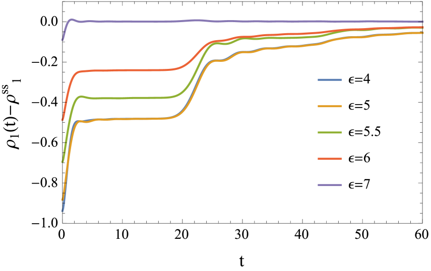
Fig. 14: (Color Online) Behavior of the time-dependent electron density at site 1, $\rho_{1}(t)$, by time for several $\epsilon$. We set the parameters as $N=20,\ V_{L}=V_{R}=6,\ \Gamma_{L}=\Gamma_{R}=\gamma=0.5$. There are three regions in the case: $\epsilon>V+2\gamma=7$, $\epsilon<V-2\gamma=5$, and $5<\epsilon<7$.

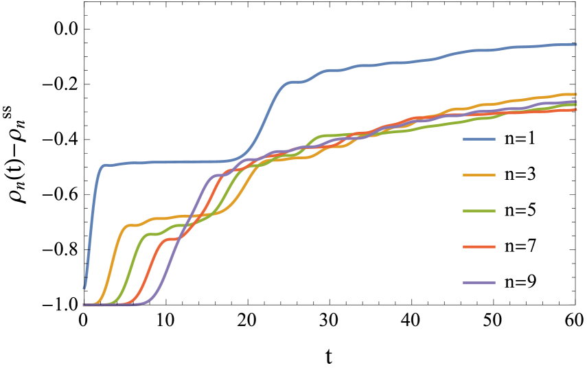
Fig. 15: (Color Online) The behavior of the time-dependent electron density $\rho_{n}(t)$ by time $t$ for several site indices $n$: $n=1,3,5,7,9$.

In Fig. 15, we numerically compute the time-dependent electron density at site 1 from the definition (29) for several $\epsilon$ and see the dependence of the two-step decay on $\epsilon$. We set the parameters as $N=20,\ V_{L}=V_{R}=6,\ \Gamma_{L}=\Gamma_{R}=\gamma=0.5$. As we expect, the electron density has two-step decay for $\epsilon<V+2\gamma$. For the case of $\epsilon<V-2\gamma$, the transient behaviors of the electron density for several $\epsilon$ are the same. We can understand this fact from the expressions (37) and (39). Because the term of on-site energy $\epsilon$ appears in (37) as a phase factor, the effect disappears in (39) by taking the norm of $A_{nm}(t)$ and therefore the behavior of the time-dependent electron density for $\epsilon<V-2\gamma$ is the same. In the case $V-2\gamma<\epsilon<V+2\gamma$, however, the behavior of the electron density changes with the on-site energy. As the energy increases to $\epsilon=V+2\gamma$, the value of the electron density decays. This is because the number of the terms $B_{nm}$ in (36) with the phase factor $2\pi i$ decreases. In the case of $\epsilon>V+2\gamma$, the electron density quickly converges towards 0. This behavior matches with our expectation obtained in the discussion of $\sum_{n}|A_{nm}|^{2}(t)$. We also see the behavior of the time-dependent electron density for several site $n$ in Fig. 15. From this figure, we can confirm that the times when the two-step decays occur change with site index according to $t_{1}=\frac{N+1-n}{2\gamma}$ and $t_{2}=\frac{N+1+n}{2\gamma}$, which are our theoretical prediction from (41).

Until now we only consider the case where there is no special eigenvalue. We study the time-dependent electron density including the effect of the special eigenvalue. Because of the special eigenvalue, a new term appears in the expression for the electron density and it changes the dependence of the time-dependent electron density on the boundary parameters. In the following analytical study, we only focus on the behavior of the $A_{nm}$ because it mainly determines the behavior of the time-dependent electron density as we see it in the discussion of the case $r,l<1$ above. For simple analysis, we consider the situation of $l=0,\ r>1$, where the special eigenvalue $\Lambda_{r}$ exists. For large $N$, we can separate the relation (13) into

$$\sum_{k}\mathbf{R}_{k}=\sum_{k:\ \mathrm{normal}}\mathbf{R}_{k}+\mathbf{R}_{\Lambda_{r}}.$$ (45)

By substituting (45) into the definition of $A_{nm}$ (37), we obtain the expression for $A_{nm}(t)$ for $l=0,\ r>1$ as

$$A_{nm} =\sum_{k:\ \mathrm{normal}}[\mathbf{R}_{k}]_{nm}e^{-i\lambda_{k}t}+[\mathbf{R}_{\Lambda_{r}}]_{nm}e^{-i\Lambda_{l}t}$$

$$\eqsim e^{-i\epsilon t}\left(h_{nm}(t,0)-(1+r^{2})(-ir)^{n+m-2(N+1)}e^{-\gamma(r-\frac{1}{r})t}\right),$$ (46)

where we only focus on the largest order of $r$. The detail of the derivation is in Appendix C. By comparing the expression (46) with the expression (40) of $A_{nm}$ for $l=0$ and $r<1$, we can see that an additional term $-(1+r^{2})(-ir)^{n+m-2(N+1)}e^{-\gamma(r-\frac{1}{r})t}$ appears due to the special eigenvalue $\Lambda_{r}$. When $n$ and $m$ are order of $O(N)$, this term remains in the limit $N\rightarrow\infty$. Because the common term $h_{nm}(t,0)$ does not depend on the boundary coupling parameter $r$, the additional term changes dependence on the boundary parameter at $r=1$ and cause an interesting behavior as we see blow.

We can see effects of the additional term in (46) from direct numerical computation of the time-dependent electron density using (29). To see the dependence on the boundary parameter, we fix $t$ at a time. At the time, we change the boundary parameter $\Gamma_{R}$ and see the dependence of the electron density on the boundary parameter. The result is Fig.17. The red points in the figure express extreme values of the graphs obtained numerically.

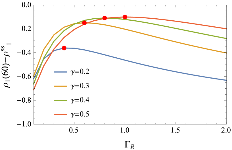
Fig. 16: (Color Online) The behavior of the time-dependent electron density at a time $\rho_{1}(60)-\rho^{ss}_{1}$ for several $\gamma$ and $\Gamma_{R}$. We set the parametrs as $N=20,\ V_{L}=V_{R}=6,\ \epsilon=3,\ \Gamma_{L}=0$. Depending on the parameters $\gamma$, the peak(red point) changes and is compatible with out expectation $\Gamma_{R}=2\gamma$ for all the cases.

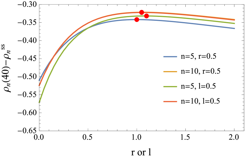
Fig. 17: (Color Online) The behavior of the time-dependent electron density $\rho_{n}(t)-\rho^{ss}_{n}$ for several site $n$ by coupling parameter $l$ or $r$. We fix $l$ when we change the parameters $r$ and vice versa. We set the parametrs as $N=20,\ V_{L}=V_{R}=6,\ \gamma=0.5,\epsilon=3$. We consider $t=40$ as a different time from that in Fig 17.

From the graphs, we can notice that the dependence on the boundary parameter, or $\frac{d\rho_{n}(t)}{dr}$, changes at $\Gamma_{R}=2\gamma$, which is compatible with our analytical expectation above. In the region where $\Gamma_{R}<2\gamma$, $\frac{d\rho_{n}(t)}{dr}$ is positive. This means that the convergence speed of the electron density to steady state becomes fast by increasing $\Gamma_{R}$ since we calculate the difference from the electron density in the steady state. This is intuitively natural result because the boundary parameter determines how easy particles can flow into the sites. In contrast, the derivative is negative for $\Gamma_{R}>2\gamma$, or the convergence speed becomes slower from the point $r=1$ by increasing the value of the boundary parameter. Unlike the case of $r<1$, this is contrary to our intuition. We can physically understand this behavior as follows. When the boundary parameter is smaller than the coupling parameter between the dots $\Gamma_{R}<2\gamma$, particles can hop to the next site from the rightmost site more easily than the rightmost site from the right reservoir $R$. Therefore, a bottleneck appears between the right most site and the right reservoir and convergence speed becomes fast by increasing the $\Gamma_{R}$. In contrast, for the case $\Gamma_{R}>2\gamma$, particles are stuck not between the rightmost site and the right reservoir but between the sites. In this situation, by increasing the boundary parameter, outflow of particles from the rightmost site to the right reservoir is likely to happen. This means that the convergence speed becomes slower by changing the boundary parameter. In this way, we can understand the change of dependence of the time-dependent electron density on the boundary parameter. We note that the behavior for $\Gamma_{R}<2\gamma$ seems not to match our theoretical prediction above, but this difference appears to be due to finite size effects. In the limit $N\rightarrow\infty$, the time-dependent electron density does not depend on boundary parameter for the case $r,l<1$ as in (46). However, in the finite case, the effect of the boundary parameter remains and the dependence exists. Finally we can check the change of dependence on the boundary parameters for the case where both boundary parameters $\Gamma_{L}$ and $\Gamma_{R}$ exist as in Fig. 17.

In this way, the dependence of time-dependent electron density on the boundary parameter changes at $r,l=1$, where the special eigenvalue of the non-hermitian matrix (8) appears. This means that we can properly manipulate speed of decay by changing boundary parameter. Though we can simply consider that the convergence speed to steady state becomes faster as we increase the boundary parameters, the fastest decay actually happens at $\Gamma_{L}=\Gamma_{R}=\gamma$. If the boundary parameters are larger than the value, the decay speed becomes slow. This fact can be useful for quantum computation, where coherence time is very important quantity.

6 Conclusion

We have investigated the $N$ tight-binding model coupled to two reservoirs with the nonequilibrium Green function including initial correlation to understand effects of the open boundaries. By carrying out concrete analytical investigation of the formal expression (2) in our case, we obtained expressions for the steady-state and the time-dependent electron density for the limit $N\rightarrow\infty$ and $\beta=\infty$. We showed that the non-hermitian matrix, which appeared in the expression of the electron density, could have special eigenvalues whose imaginary parts did not vanish even in the thermodynamic limit $N\rightarrow\infty$. From the simple expression of the electron density in the steady state, we analytically showed that the special eigenvalues did not affect the qualitative behavior of the electron density and the phase transition which has been observed for the isolated tight-binding model also existed in our open case. In contrast, we found that the open boundaries affect the qualitative behavior of the time-dependent electron density. From the expression of the time-dependent electron density, we saw that the electron density has the two-step decay caused by open boundaries for the region where the on-site energy is not large enough $\epsilon<V+2\gamma$. Because of the boundary effect, particles flow and the time lag between flow of particles from the left and the right reservoir causes the two-step decay as in Fig. 13. In addition, we showed that the dependence of convergent speed on the boundary couplings changed by the special eigenvalues. Because the boundary parameters determine the existence of the special eigenvalues, the qualitative change of the convergent speed is a result of the open boundaries.

Until now, we have considered the regime where the Coulomb interaction between electrons are irrelevant. Therefore, it is interesting to investigate the transient dynamics of the model including the Coulomb interaction and understand the effect of the interaction to the dynamics.

Appendix A About Eigenvalue and Eigenvector of $\mathbf{h}^{eff}$

A.1 Derivation of the Characteristic Equation

In this subsection, we derive the characteristic equation of $\mathbf{h}^{eff}$ (5). The characteristic equation of $\mathbf{h}^{eff}$ (5) is written as

$$\begin{pmatrix}\epsilon-\frac{i}{2}\Gamma_{L}&\gamma&0&\cdots&&&&\\ \gamma&\epsilon&\gamma&0&\cdots&&&\\ 0&\gamma&\epsilon&\gamma&\cdots&&&\\ \vdots&&&&&&&\\ 0&\cdots&&&&0&\gamma&\epsilon-i\frac{i}{2}\Gamma_{R}\\ \end{pmatrix}\begin{pmatrix}e_{1}\\ e_{2}\\ \vdots\\ \\ e_{N}\\ \end{pmatrix}=\lambda\begin{pmatrix}e_{1}\\ e_{2}\\ \vdots\\ \\ e_{N}\\ \end{pmatrix}.$$

By introducing $e_{0}=-i\frac{\Gamma_{L}}{2\gamma}e_{1}=-ile_{1}$ and $e_{N+1}=-i\frac{\Gamma_{R}}{2\gamma}e_{N}=-ire_{N}$, the characteristic equation is expressed as

$$\begin{pmatrix}\gamma&\epsilon&\gamma&\cdots&&&&\\ 0&\gamma&\epsilon&\gamma&\cdots&&&\\ 0&0&\gamma&\epsilon&\cdots&&&\\ \vdots&&&&&&&\\ 0&\cdots&&&0&\gamma&\epsilon&\gamma\\ \end{pmatrix}\begin{pmatrix}e_{0}\\ e_{1}\\ \vdots\\ \\ e_{N+1}\\ \end{pmatrix}=\lambda\begin{pmatrix}e_{1}\\ e_{2}\\ \vdots\\ \\ e_{N}\\ \end{pmatrix},$$

or, in the form of the recurrence relation,

$$\gamma e_{n-1}+\epsilon e_{n}+\gamma e_{n+1}=\lambda e_{n},$$ (A.1)

for $n=1,2\cdots N$. To obtain the solution of the recurrence relation Eq. (A.1), we rewrite Eq. (A.1) in a form of $e_{n+1}-\alpha e_{n}=\beta(e_{n}-\alpha e_{n-1})$. By comparing the coefficients $e_{n+1}-\alpha e_{n}=\beta(e_{n}-\alpha e_{n-1})$ with Eq. (A.1), we obtain the following relation

$$\alpha+\beta=\frac{\lambda-\epsilon}{\gamma},\ \alpha\beta=1.$$ (A.2)

Therefore, $\alpha$ and $\beta$ which satisfy the relation (A.2) are expressed as $\alpha,\beta=(\lambda-\epsilon)/2\gamma\pm\sqrt{\left((\lambda-\epsilon)/2\gamma\right)^{2}-1}$. Here we use the fact $\beta\neq\alpha$, which we can prove. Using $\alpha$ and $\beta$, we can obtain the following expression

$$e_{n+1}-\alpha e_{n} =\beta^{n}(e_{1}-\alpha e_{0})$$

$$=(\beta^{n}+\beta^{n-1}il)e_{1},$$

where we use the boundary condition $e_{0}=-ile_{1}$ and $\alpha\beta=1$ from the relation (A.2). In the similar manner, we can obtain the relation $e_{n+1}-\beta e_{n}=(\alpha^{n}+\alpha^{n-1}i\beta l)e_{1}$. By taking the difference of the two relations, we obtain

$$(\beta-\alpha)e_{n}=\{\beta^{n}-\alpha^{n}+il(\beta^{n-1}-\alpha^{n-1})\}e_{1}$$ (A.3)

Until now, we use only one of the boundary condition $e_{0}=-ile_{1}$. Therefore, Eq. A.3 have to satisfy the other boundary condition, $e_{N+1}=-ire_{N}$. From this condition, we obtain

$$\frac{e_{N+1}}{e_{N}}=\frac{\beta^{n+1}-\alpha^{n+1}+il(\beta^{n}-\alpha^{n})}{\beta^{n}-\alpha^{n}+il(\beta^{n-1}-\alpha^{n-1})}=-ir,$$

where we use $e_{1}\neq 0$. If $e_{1}=0$, then $e_{n}=0$ for $n=1,2,\cdots N$ holds from the boundary condition $e_{1}=-ile_{0}$ and the recurrence relation (A.1), which contradicts the definition of eigenvector. The equation is expressed as

$$\beta^{n+1}-\alpha^{n+1}+i(l+r)(\beta^{n}-\alpha^{n})-rl(\beta^{n-1}-\alpha^{n-1})=0,$$ (A.4)

is the same as Eq. (6). Eigenvalues are determined from $\alpha$ and $\beta$ through the relation (A.2).

A.2 Derivation of the Expression for $\mathbf{R}_{k}$

In this subsection, we derive Eq. (16) and Eq. (17). By definition of $\mathbf{R}_{k}$ in Eq. (14), we have

$$[\mathbf{R}_{k}]_{nm} =\left[\frac{\mathbf{r}_{k}\mathbf{r}^{t}_{k}}{\mathbf{r}^{t}_{k}\cdot\mathbf{r}_{k}}\right]_{nm}$$

$$=\frac{(\sin n\Theta_{k}+il\sin(n-1)\Theta_{k})(\sin m\Theta_{k}+il\sin(m-1)\Theta_{k}))}{\sum^{N}_{n=1}(\sin n\Theta_{k}+il\sin(n-1)\Theta_{k})^{2}}.$$ (A.5)

We can calculate denominator in (A.5) as follows.

$$\sum^{N}_{n=1}(\sin n\Theta_{k}+il\sin(n-1)\Theta_{k})^{2} =\sum^{N}_{n=1}\sin^{2}n\Theta_{k}-l^{2}\sin^{2}(n-1)\Theta_{k}+i2l\sin n\Theta_{k}\sin(n-1)\Theta_{k}$$

$$=\frac{1}{2}(1-\cos 2n\Theta_{k})-\frac{l^{2}}{2}(1-\cos(2n-1)\Theta_{k})$$

$$\quad+i2l\frac{-1}{2}(\cos 2(n-1)\Theta_{k}-\cos 2\Theta_{k})$$

$$=\frac{N}{2}(1-l^{2}+i2l\cos\Theta_{k})$$

$$\quad-\frac{1}{2}\sum^{N}_{n=1}(\cos 2n\Theta_{k}-l^{2}\cos 2(n-1)\Theta_{k}+i2l\cos(2n-1)\Theta_{k}).$$ (A.6)

Here we use the relations $\sum^{N}_{n=0}T_{2n}(z)=\frac{1}{2}(1+U_{2N}(z))$ and $\sum^{N}_{n=0}T_{2n+1}(z)=\frac{1}{2}U_{2N+1}(z)$. $T_{n}(\cos\theta)=\cos n\theta$ is the Chebyshev polynomial of the first kind. By applying these relations to Eq. (A.6), we obtain the expression for the denominator of Eq. (A.5)

$$\sum_{n}(\sin n\Theta_{k}+il\sin(n-1)\Theta_{k})^{2} =\frac{N}{2}(1-l^{2}+i2l\cos\Theta_{k})$$

$$\quad-\frac{1}{4}(-1-l^{2}+U_{2N}(\cos\Theta_{k})-l^{2}U_{2(N-1)}(\cos\Theta_{k})$$

$$\qquad+i2lU_{2N-1}(\cos\Theta_{k})),$$ (A.7)

We can prove that the second term in Eq. (A.7) is order of $O(N^{0})$. Therefore, for large $N$, we obtain Eq. (16)

$$[\mathbf{R}_{k}]_{nm}\eqsim\frac{2}{N}\frac{(\sin n\Theta_{k}+il\sin(n-1)\Theta_{k})(\sin m\Theta_{k}+il\sin(m-1)\Theta_{k}))}{1-l^{2}+i2l\cos\Theta_{k}}.$$ (A.8)

Next we prove the expression of $\mathbf{r}^{(n)}_{\Lambda_{l}}$ and $\mathbf{R}_{\Lambda_{l}}$, or Eq. (15) and Eq. (17). To calculate Eq. (15), we need the expression of $\sin\Theta_{k}$ for the normalized special eigenvalue $\alpha=-il$, which we represent as $\sin\Theta_{\Lambda_{l}}$. Here we use the fact that the expression for the characteristic equation (12) can be obtained by substituting $\alpha=e^{i\Theta_{k}}$ into Eq. (7). Therefore, $\sin n\Theta_{\Lambda_{l}}$ is expressed as

$$\sin n\Theta_{\Lambda_{l}} =\frac{(-il)^{n}-(-il)^{-n}}{2i}.$$ (A.9)

By substituting the relation (A.9) into (14), we obtain the expression of the eigenvector for the special eigenvalue, Eq. (15),

$$\mathbf{r}^{(n)}_{\Lambda_{l}}=-\frac{(-il)^{-n+1}}{2}(l+\frac{1}{l}).$$

From the expression for Eq. (15), the denominator of for large $N$ is calculated as

$$\mathbf{r}^{t}_{\Lambda_{l}}\mathbf{r}_{\Lambda_{l}}\eqsim\frac{1}{4}(1+l^{2}).$$ (A.10)

By substituting (15) and (A.10) into the definition of $\mathbf{R}_{k}$ in Eq. (13), we obtain

$$[\mathbf{R}_{\Lambda_{l}}]_{nm}\eqsim-(1+l^{2})(-il)^{-(n+m)},$$

which is Eq. (17).

Appendix B Derivation of Eq. (23)

In this section, we prove

$$\rho^{ss}_{phase} :=-i\sum_{k,l}(\lambda_{k}-\lambda^{*}_{l})^{-1}\mathbf{R}_{k}\mathbf{\Gamma}\mathbf{R}^{*}_{l}$$

$$=\mathbf{1},$$ (B.1)

and Eq. (23) in Section 3. We can prove Eq. (B.1) as follows.

$$\rho^{ss}_{phase} =-i\sum_{k,l}(\lambda_{k}-\lambda^{*}_{l})^{-1}\mathbf{R}_{k}\mathbf{\Gamma}\mathbf{R}^{*}_{l}$$

$$=-i\sum_{l}(\mathbf{h}^{eff}-\lambda^{*}_{l}\mathbf{1})^{-1}\mathbf{\Gamma}\mathbf{R}^{*}_{l}$$

$$=2\sum_{l}(\mathbf{h}^{eff}-\lambda^{*}_{l}\mathbf{1})^{-1}(\mathbf{h}^{eff}-\mathbf{h})\mathbf{R}^{*}_{l},$$

where we use $\sum_{k}\mathbf{R}_{k}=1$ from the first line to the second line. From the second line to the third line, we apply the relation $\mathbf{h}^{eff}=\mathbf{h}-\frac{i}{2}\mathbf{\Gamma}$. The expression is written as

$$\rho^{ss}_{phase} =2\sum_{l}(\mathbf{h}^{eff}-\lambda^{*}_{l}\mathbf{1})^{-1}((\mathbf{h}^{eff}-\lambda^{*}_{l}\mathbf{1})+(\lambda^{*}_{l}\mathbf{1}-\mathbf{h}))\mathbf{R}^{*}_{l}$$

$$=2\sum_{l}\{\mathbf{1}+(\mathbf{h}^{eff}-\lambda^{*}_{l}\mathbf{1})^{-1}(\lambda^{*}_{l}\mathbf{1}-\mathbf{h})\}\mathbf{R}^{*}_{l}$$

$$=2\mathbf{1}+2\sum_{l}(\mathbf{h}^{eff}-\lambda^{*}_{l}\mathbf{1})^{-1}((\mathbf{h}^{eff})^{*}-\mathbf{h})\mathbf{R}^{*}_{l}$$

$$=2\mathbf{1}+i\sum_{l}(\mathbf{h}^{eff}-\lambda^{*}_{l}\mathbf{1})^{-1}\mathbf{\Gamma}\mathbf{R}^{*}_{l}$$

$$=2\mathbf{1}-\rho^{ss}_{phase},$$ (B.2)

In the first line, we insert the identity $-\lambda^{*}_{l}\mathbf{1}+\lambda^{*}_{l}\mathbf{1}=0$. From the fourth line to final line, we use the definition of $\rho^{ss}_{phase}$ in Eq. (B.1). Eq. (B.2) shows that Eq. (B.1) holds. In a similar way, we can prove Eq. (23). We start from Eq. (22),

$$\mathbf{\rho}^{ss} =1+\frac{1}{2\pi}\sum_{\alpha}\sum_{k,l}\left[\mathbf{R}_{k}\mathbf{\Gamma}_{\alpha}\left(\mathbf{R}_{l}\right)^{*}\right]\frac{1}{\lambda_{k}-\lambda^{*}_{l}}(\log(V_{\alpha}-\lambda_{k})-\log(V_{\alpha}-\lambda^{*}_{l}))$$

$$=:1+\sum_{\alpha}\mathbf{\rho}^{ss}_{\alpha,1}+\mathbf{\rho}^{ss}_{\alpha,2}.$$ (B.3)

We can rewrite $\mathbf{\rho}^{ss}_{L,1}$ as

$$\mathbf{\rho}^{ss}_{L,1} =\frac{1}{2\pi}\sum_{k,l}\mathbf{R}_{k}\mathbf{\Gamma}_{\alpha}\mathbf{R}^{*}_{l}\frac{1}{\lambda_{k}-\lambda^{*}_{l}}\log(V_{L}-\lambda_{k})$$

$$=\frac{1}{2\pi}\sum_{l}\log(V_{L}-\mathbf{h}^{eff})(\mathbf{h}^{eff}-\lambda^{*}_{l}\mathbf{1})^{-1}\mathbf{\Gamma}_{L}\mathbf{R}^{*}_{l}$$

$$=\frac{1}{2\pi}\sum_{l}\log(V_{L}-\mathbf{h}^{eff})(\mathbf{h}^{eff}-\lambda^{*}_{l}\mathbf{1})^{-1}(\mathbf{\Gamma}-\mathbf{\Gamma}_{R})\mathbf{R}^{*}_{l},$$

where we use the definition $\mathbf{\Gamma}=\mathbf{\Gamma}_{L}+\mathbf{\Gamma}_{R}$. With the definition $\mathbf{h}^{eff}=\mathbf{h}-\frac{i}{2}\mathbf{\Gamma}$ , we have

$$\mathbf{\rho}^{ss}_{L,1} =\frac{1}{2\pi}\sum_{l}\log(V_{L}-\mathbf{h}^{eff})(\mathbf{h}^{eff}-\lambda^{*}_{l}\mathbf{1})^{-1}\{2i(\mathbf{h}^{eff}-\lambda^{*}_{l}\mathbf{1}+\lambda^{*}_{l}\mathbf{1}-\mathbf{h}+\frac{i}{2}\mathbf{\Gamma}_{R})\}\mathbf{R}^{*}_{l}$$

$$=\frac{i}{\pi}\sum_{l}\log(V_{L}-\mathbf{h}^{eff})\{\mathbf{1}+(\mathbf{h}^{eff}-\lambda^{*}_{l}\mathbf{1})^{-1}(\lambda^{*}_{l}\mathbf{1}-\mathbf{h}+\frac{i}{2}\mathbf{\Gamma}_{R})\}\mathbf{R}^{*}_{l}$$

$$=\frac{i}{\pi}\sum_{l}\log(V_{L}-\mathbf{h}^{eff})\{\mathbf{1}+(\mathbf{h}^{eff}-\lambda^{*}_{l}\mathbf{1})^{-1}((\mathbf{h}^{eff})^{*}-\mathbf{h}+\frac{i}{2}\mathbf{\Gamma}_{R})\}\mathbf{R}^{*}_{l}$$

$$=\frac{i}{\pi}\log(V_{L}-\mathbf{h}^{eff})-\mathbf{\rho}^{ss}_{L,1}-\frac{1}{\pi}\sum_{l}\log(V_{L}-\mathbf{h}^{eff})(\lambda_{k}\mathbf{1}-\lambda^{*}_{l})^{-1}\mathbf{\Gamma}_{R}\mathbf{R}^{*}_{l}.$$

We insert $-\lambda^{*}_{l}\mathbf{1}+\lambda^{*}_{l}\mathbf{1}=0$ in the first line. From the third line to the final line, we use $(\mathbf{h}^{eff})^{*}-\mathbf{h}+\frac{i}{2}\mathbf{\Gamma}_{R}=\frac{i}{2}\mathbf{\Gamma}_{L}+i\mathbf{\Gamma}_{R}$. Therefore, we obtain

$$\mathbf{\rho}^{ss}_{L,1}=\frac{i}{2\pi}\log(V_{L}-\mathbf{h}^{eff})-\frac{1}{2\pi}\sum_{l}\log(V_{L}-\mathbf{h}^{eff})(\lambda_{k}\mathbf{1}-\lambda^{*}_{l})^{-1}\mathbf{\Gamma}_{R}\mathbf{R}^{*}_{l}$$ (B.4)

By carrying out the same calculation for $\mathbf{\rho}^{ss}_{R,1}$, $\mathbf{\rho}^{ss}_{1}$ is expressed as

$$\mathbf{\rho}^{ss}_{1} =\sum_{\alpha}\mathbf{\rho}^{ss}_{\alpha,1}$$

$$=\frac{i}{2\pi}\sum_{\alpha}\log(V_{\alpha}-\mathbf{h}^{eff})-\frac{1}{2\pi}\sum_{k,l}\mathbf{R}_{k}\frac{1}{\lambda_{k}-\lambda^{*}_{l}}(\log(V_{L}-\lambda_{k})\mathbf{\Gamma}_{R}+\log(V_{R}-\lambda_{k})\mathbf{\Gamma}_{L})\mathbf{R}^{*}_{l}.$$ (B.5)

In a similar way, we can obtain an expression of $\mathbf{\rho}^{ss}_{2}$

$$\mathbf{\rho}^{ss}_{2} =-\frac{i}{2\pi}\sum_{\alpha}\log(V_{\alpha}-(\mathbf{h}^{eff})^{*})+\frac{1}{2\pi}\sum_{k,l}\mathbf{R}_{k}\frac{1}{\lambda_{k}-\lambda^{*}_{l}}(\log(V_{L}-\lambda^{*}_{l})\mathbf{\Gamma}_{R}+\log(V_{R}-\lambda^{*}_{l})\mathbf{\Gamma}_{L})\mathbf{R}^{*}_{l}.$$ (B.6)

By substituting (B.5) and (B.6) for (B.3), we have the expression for the electron density in the steady state, (23)

$$\mathbf{\rho}^{ss} =1+\frac{i}{2\pi}\sum_{\alpha}(\log(V_{\alpha}-\mathbf{h}^{eff})-\log(V_{\alpha}-(\mathbf{h}^{eff})^{*}))$$

$$\quad-\frac{1}{2\pi}\sum_{k,l}\mathbf{R}_{k}\frac{1}{\lambda_{k}-\lambda^{*}_{l}}\bigl{(}(\log(V_{L}-\lambda_{k})-\log(V_{L}-\lambda^{*}_{l}))\mathbf{\Gamma}_{R}$$

$$\qquad+(\log(V_{R}-\lambda_{k})-\log(V_{R}-\lambda^{*}_{l}))\mathbf{\Gamma}_{L}\bigr{)}\left(\mathbf{R}_{l}\right)^{*}.$$

Appendix C About the derivation of the Analytical Expression for the Time-dependent Electron Density

C.1 Derivation of the Expression of $F_{2}(t,z)$ for $\beta=\infty$

In this appendix, we first derive (31), the representation of $F_{2}(t,z)$ for $\beta=\infty$. By definition, we have the following expression

$$F_{2}(t,z) =\int^{0}_{-\infty}\frac{d\omega}{2\pi}\frac{e^{i\omega t}}{\omega-z}$$

$$=\int^{0}_{-\infty}\frac{d\omega}{2\pi}\frac{\cos\omega}{\omega-tz}+i\int^{0}_{-\infty}\frac{d\omega}{2\pi}\frac{\sin\omega}{\omega-tz}$$

$$=\frac{1}{2\pi}(-g(tz)+if(tz)),$$ (C.1)

where we define $g(z)=\int^{\infty}_{0}\frac{\cos\omega}{\omega+z}$ and $f(z)=\int^{\infty}_{0}\frac{\sin\omega}{\omega+z}$. These functions are expressed with the first-order exponential integral with its principal value as

$$g(z)-if(z)=e^{iz}E_{1}(iz)$$

Note that this expression only holds for $-\pi<\mathrm{arg}z<\frac{\pi}{2}$. By substituting the relation into (C.1), we obtain

$$F_{2}(t,z)=-\frac{e^{itz}}{2\pi}E_{1}(itz).$$ (C.2)

for $-\pi<\mathrm{arg}z<\frac{\pi}{2}$. For the case of $\frac{\pi}{2}<\mathrm{arg}z<\pi$, or $\mathrm{Re}z<0$ and $\mathrm{Im}z>0$, $E_{1}(itz)$ changes to $E_{1}(itz)-2\pi i$. We understand this as follows. The exponential integral of first order with its principal value is expressed as

$$E_{1}(z)=-\gamma-\mathrm{Log}z+\mathrm{Ein}(z),$$

where $\gamma$ is the Euler-Mascheroni constant and $\mathrm{Ein}(z)=\int^{z}_{0}dt\frac{1-e^{-t}}{t}$ is holomorphic function. Therefore, the term $-2\pi i$ arises from $\log iz$ in the general value of $E_{1}(z)$ when $\mathrm{Re}z<0$ and $\mathrm{Im}z>0$. This is because $iz$ cross the branch of negative real line. Therefore, we obtain the expression (31).

C.2 Derivation of the Expression for $\mathbf{\rho}^{(1,1)}_{n}(t)$, $\mathbf{\rho}^{(1,2)}_{n}(t)$, and $\mathbf{\rho}^{(2)}_{n}(t)$

In this appendix, we derive (35), (36), (42) and (46), which are the expression of $\mathbf{\rho}^{(1,1)}_{n}(t)$, $\mathbf{\rho}^{(1,2)}_{n}(t)$, $\mathbf{\rho}^{(2)}_{n}(t)$ for $0<l<1$, and $A_{nm}(t)$ for $l=0,\ r>1$ respectively. First we show the derivation of $\mathbf{\rho}^{(1,1)}_{n}(t)$ for $l=0$ case, which enable us to understand the derivation for $0<l<1$ easily. We start from the definition of $\mathbf{\rho}^{(1,1)}_{n}(t)$ in (33). We use the expression of $[\mathbf{R_{k}}]_{nn}$ in (16) and the eigenvalue $\lambda_{k}\eqsim\epsilon+2\gamma\cos\Theta_{k}$ for large $N$. By substituting these expressions and (31) into the definition and taking $N\rightarrow\infty$, we have

$$\mathbf{\rho}^{(1,1)}_{n}(t) =-i\sum_{k}[\mathbf{R}_{k}]_{nn}e^{-i(\lambda_{k}-V)t}F_{2}(t,\lambda_{k}-V)$$

$$=-i\sum_{k}\frac{2}{N}\sin^{2}n\theta e^{-i(\epsilon+2\gamma\cos\Theta_{k}-V)t}\times$$

$$\quad-\frac{e^{it(\epsilon+2\gamma\cos\Theta_{k}-V)}}{2\pi}E_{1}(it(\epsilon+2\gamma\cos\Theta_{k}-V))$$

$$\xrightarrow{N\rightarrow\infty}\frac{i}{2\pi}\frac{2}{\pi}\int^{\pi}_{0}d\theta\sin^{2}n\theta E_{1}(it(\epsilon+2\gamma\cos\theta-V)),$$ (C.3)

where we use $\Delta\Theta_{k}=\Theta_{k}-\Theta_{k-1}=\frac{\pi}{N}$ for large $N$. To calculate the $\theta$-integral in (C.3), we use the expression of the exponential integral $E_{1}(itx)=\int^{\infty}_{t}ds\frac{e^{-ixs}}{s}$. By substituting the expression into (C.3), we have the following expression

$$\mathbf{\rho}^{(1,1)}_{n}(t) =\frac{i}{2\pi}\frac{2}{\pi}\int^{\pi}_{0}d\theta\sin^{2}n\theta\int^{\infty}_{t}ds\frac{e^{-is(\epsilon+2\gamma\cos\theta-V)}}{s}$$

$$=\frac{i}{2\pi}\frac{1}{\pi}\int^{\pi}_{-\pi}d\theta\sin^{2}n\theta\int^{\infty}_{t}ds\frac{e^{-is(\epsilon-V)}}{s}e^{-is2\gamma\cos\theta}$$

$$=\frac{i}{2\pi}\frac{1}{\pi}\oint_{C}\frac{dz}{iz}\left(\frac{1}{2i}(z^{n}-z^{-n})\right)^{2}\int^{\infty}_{t}ds\frac{e^{-is(\epsilon-V)}}{s}e^{-is2\gamma\frac{1}{2}(z+z^{-1})}$$

$$=\frac{i}{2\pi}\frac{-1}{4\pi i}\int^{\infty}_{t}ds\frac{e^{-is(\epsilon-V)}}{s}\oint_{C}\frac{dz}{z}(z^{n}-z^{-n})^{2}e^{-is\gamma(z+z^{-1})},$$ (C.4)

where the contour $C$ is the unit circle. From the first line to the second line, we use the fact that the integrand is even function. From the second to the third line, we change variable from $\theta$ to $z=e^{i\theta}$. We can calculate the complex integral in (C.4]) by using $e^{\frac{1}{2}s(z+\frac{1}{z})}=\sum^{\infty}_{m=-\infty}I_{m}(s)z^{m}$, where $I_{n}(x)$ is the modified Bessel function, and the residue theorem. With this relation, we can obtain the concrete expression of the complex integral as

$$\oint_{C}\frac{dz}{z}(z^{n}-z^{-n})^{2}e^{-is\gamma(z+\frac{1}{z})} =2\pi i\mathrm{Res}(z=0)$$

$$=2\pi i(I_{-2n}(-2i\gamma s)-2I_{0}(-2i\gamma s)+I_{2n}(-2i\gamma s))$$

$$=4\pi i(I_{2n}(-2i\gamma s)-I_{0}(-2i\gamma s)),$$ (C.5)

where we use the relation $I_{n}(z)=I_{-n}(z)$ from the second line to the third line. Using this result, we arrive at the expression of $\mathbf{\rho}^{(1,1)}_{n}(t)$ for $r=0$

$$\mathbf{\rho}^{(1,1)}_{n}(t) =\frac{i}{2\pi}\frac{-1}{4\pi i}\int^{\infty}_{t}ds\frac{e^{-is(\epsilon-V)}}{s}2\pi i\mathrm{Res}(z=0)$$

$$=\frac{i}{2\pi}\frac{-1}{4\pi i}\int^{\infty}_{t}ds\frac{e^{-is(\epsilon-V)}}{s}4\pi i(I_{2n}(-2i\gamma s)-I_{0}(-2i\gamma s))$$

$$=\frac{i}{2\pi}\ \int^{\infty}_{t}ds\frac{e^{-is(\epsilon-V)}}{s}(I_{0}(-2i\gamma s)-I_{2n}(-2i\gamma s)).$$

We calculate $\mathbf{\rho}^{(1,1)}_{n}(t)$ for the case of $0<l<1$, (35). In the same way as deriving the first line in (C.4), we have the following expression for $0<l<1$

$$\mathbf{\rho}^{(1,1)}_{n}(t) =\frac{i}{2\pi}\frac{2}{\pi}\int^{\pi}_{0}d\theta\frac{(\sin n\theta+il\sin(n-1)\theta)^{2}}{1-l^{2}+2il\cos\theta}E_{1}(it(\epsilon+2\gamma\cos\theta-V))$$

$$=\frac{i}{2\pi}\frac{2}{\pi}\int^{\pi}_{0}d\theta\frac{(\sin n\theta+il\sin(n-1)\theta)^{2}}{1-l^{2}+2il\cos\theta}\int^{\infty}_{t}ds\frac{e^{-is(\epsilon+2\gamma\cos\theta-V)}}{s}$$

$$=\frac{i}{2\pi}\frac{2}{\pi}\int^{\infty}_{t}ds\frac{e^{-is(\epsilon-V)}}{s}\int^{\pi}_{0}d\theta\frac{(\sin n\theta+il\sin(n-1)\theta)^{2}}{1-l^{2}+2il\cos\theta}e^{-is2\gamma\cos\theta},$$ (C.6)

In contrast to (C.3), the term $1-l^{2}+2il\cos\theta$ appears in the integration. To carry out $\theta$-integral in (C.6), we express $e^{-is2\gamma\cos\theta}$ in (C.6) as

$$\mathrm{exp}\left[-is2\gamma\cos\theta\right] =\mathrm{exp}\left[-s\frac{\gamma}{l}\left((1-l^{2})-(1-l^{2})+2il\cos\theta\right)\right]$$

$$=\mathrm{exp}\left[s\frac{\gamma}{l}(1-l^{2})\right]\mathrm{exp}\left[-s\frac{\gamma}{l}((1-l^{2})+2il\cos\theta)\right]$$

$$=e^{s\frac{\gamma}{l}(1-l^{2})}\int^{\infty}_{s}du\frac{\gamma}{l}(1-l^{2}+2il\cos\theta)e^{-u\frac{\gamma}{l}(1-l^{2}+2il\cos\theta)}$$

$$=\frac{\gamma}{l}(1-l^{2}+2il\cos\theta)\int^{\infty}_{s}due^{\gamma(l-\frac{1}{l})(u-s)}e^{-iu2\gamma\cos\theta},$$ (C.7)

By substituting (C.7) into (C.6) and carrying out the similar calculation as (C.5), we obtain

$$\mathbf{\rho}^{(1,1)}_{n}(t) =\frac{i}{2\pi}\frac{2}{\pi}\int^{\infty}_{t}ds\frac{e^{-is(\epsilon-V)}}{s}\int^{\pi}_{0}d\theta(\sin n\theta+il\sin(n-1)\theta)^{2}\times$$

$$\qquad\frac{\gamma}{l}\int^{\infty}_{s}due^{\gamma(l-\frac{1}{l})(u-s)}e^{-iu2\gamma\cos\theta}$$

$$=\frac{i}{2\pi}\frac{\gamma}{l}\int^{\infty}_{t}ds\frac{e^{-is(\epsilon-V)}}{s}\int^{\infty}_{s}due^{\gamma(l-\frac{1}{l})(u-s)}\times$$

$$\qquad\frac{2}{\pi}\int^{\pi}_{0}d\theta(\sin n\theta+il\sin(n-1)\theta)^{2}e^{-iu2\gamma\cos\theta}$$

$$=\frac{i}{2\pi}\frac{\gamma}{l}\int^{\infty}_{t}ds\frac{e^{-is(\epsilon-V)}}{s}\int^{\infty}_{s}due^{\gamma(l-\frac{1}{l})(u-s)}h_{nn}(u,l),$$ (C.8)

which is (35). Next we calculate the expression for (36). For the case $\epsilon<V+2\gamma$, by substituting the expression for $F_{2}(z)$, (31), into the definition of $\mathbf{\rho}^{(1,2)}(t)$, we obtain

$$\mathbf{\rho}^{(1,2)}_{n}(t) =i\sum_{k,l}\sum_{m}[\mathbf{R}_{k}]_{nm}[\mathbf{R}^{*}_{l}]_{mn}e^{-i(\lambda_{k}-V)t}F_{2}(t,\lambda^{*}_{l}-V)$$

$$=-i\sum_{k,l}\sum_{m}[\mathbf{R}_{k}]_{nm}[\mathbf{R}^{*}_{l}]_{mn}e^{-i(\lambda_{k}-V)t}\frac{e^{it(\lambda^{*}_{l}-V)}}{2\pi}E_{1}(it(\lambda^{*}_{l}-V))$$

$$=-\frac{i}{2\pi}\sum_{k}[\mathbf{R}_{k}]_{nm}e^{-i\lambda_{k}t}\sum_{l}[\mathbf{R}^{*}_{l}]_{mn}e^{i\lambda^{*}_{l}t}E_{1}(it(\lambda^{*}_{l}-V))$$

$$=-\frac{i}{2\pi}\sum^{N}_{m=1}A_{nm}(t)B_{mn}(t),$$

where $A_{nm}(t)$ and $B_{mn}(t)$ are defined in (37) and (38) respectively. By using the expression of $[\mathbf{R_{k}}]_{nn}$ in (16) and the eigenvalue $\lambda_{k}\eqsim\epsilon+2\gamma\cos\Theta_{k}$, we can obtain the following representations of $A_{nm}(t)$ and $B_{mn}(t)$ for $0<l<1$ in $N\rightarrow\infty$ as

$$A_{nm}(t)=\frac{2}{\pi}\int^{\pi}_{0}d\theta\frac{(\sin n\theta+il\sin(n-1)\theta)(\sin m\theta+il\sin(m-1)\theta)}{1-l^{2}+2il\cos\theta}e^{-i(\epsilon+2\gamma\cos\theta)t},$$

$$B_{mn}(t)=\frac{2}{\pi}\int^{\pi}_{0}d\theta\frac{(\sin m\theta-il\sin(m-1)\theta)(\sin n\theta-il\sin(n-1)\theta)}{1-l^{2}-2il\cos\theta}e^{i(\epsilon+2\gamma\cos\theta)t}E_{1}(it(\epsilon+2\gamma\cos\theta-V).$$

By carrying out the calculation in the same way as (C.4) and (C.8), we can obtain the expressions of $A_{nm}(t)$ and $B_{mn}(t)$ as

$$A_{nm}(t)=\frac{\gamma}{l}e^{-i\epsilon t}\int^{\infty}_{t}dse^{\gamma(l-\frac{1}{l})(s-t)}h_{nm}(s,l),$$ (C.9)

$$B_{mn}(t)=\frac{\gamma}{l}e^{i\epsilon t}\int^{\infty}_{t}ds\frac{e^{-is(\epsilon-V)}}{s}\int^{s}_{-\infty}due^{-\gamma(l-\frac{1}{l})(u-s)}h^{*}_{mn}(u-t,l).$$

which are (36). In a similar way, we can derive the expression of $\mathbf{\rho}^{(2)}_{n}(t)$, (44) as shown in Section 5. In this appendix, we derive the expression of the third line in (42). We can express the fraction in the definition as

$$\frac{V^{2}}{(\omega-\lambda_{k})(\omega+V-\lambda_{k})(\omega+V-\lambda^{*}_{l})(\omega-\lambda^{*}_{l})}$$

$$=\left(\frac{1}{\omega-\lambda_{k}}-\frac{1}{\omega+V-\lambda_{k}}\right)\left(\frac{1}{\omega-\lambda^{*}_{l}}-\frac{1}{\omega+V-\lambda^{*}_{l}}\right)$$

$$=\frac{1}{\lambda_{k}-\lambda^{*}_{l}}\left(\frac{1}{\omega-\lambda_{k}}-\frac{1}{\omega-\lambda^{*}_{l}}+\frac{1}{\omega+V-\lambda_{k}}-\frac{1}{\omega+V-\lambda^{*}_{l}}\right)$$

$$\qquad-\frac{1}{\lambda_{k}-\lambda^{*}_{l}-V}\left(\frac{1}{\omega-\lambda_{k}}-\frac{1}{\omega+V-\lambda^{*}_{l}}\right)$$

$$\qquad+\frac{1}{\lambda_{k}-\lambda^{*}_{l}+V}\left(\frac{1}{\omega-\lambda^{*}_{l}}-\frac{1}{\omega+V-\lambda_{k}}\right)$$ (C.10)

When $V\gg|\lambda_{k}-\lambda^{*}_{l}|\eqsim 4\gamma$ holds and we ignore the term of $O(\frac{1}{V})$, the second and the third terms vanish after the integration of $\omega$. Therefore, we can reproduce the final line of (42).

Finally, we derive the expression for $A_{nm}(t)$ for $l=0,r>1$, where there is a special eigenvalue $\Lambda_{r}$. For large $N$, we can calculate $\mathbf{R}_{\Lambda_{r}}$ as

$$[\mathbf{R}_{\Lambda_{r}}]_{nm} =\frac{\sin n\Theta_{\Lambda_{r}}\sin m\Theta_{\Lambda_{r}}}{\sum^{N}_{k=1}\sin^{2}k\Theta_{\Lambda_{r}}}$$

$$=\frac{(-ir)^{n}-(-ir)^{-n}}{2i}\frac{(-ir)^{m}-(-ir)^{-m}}{2i}\frac{1}{\sum_{k}\left(\frac{(-ir)^{k}-(-ir)^{-k}}{2i}\right)^{2}}$$

$$\eqsim-(1+r^{2})(-ir)^{n+m-2(N+1)}.$$ (C.11)

From the first line to the second line, we use $\sin n\Theta_{\Lambda_{r}}=\frac{(-ir)^{n}-(-ir)^{-n}}{2i}$, which we can obtain in the similar way of (A.9). In the final line, we ignore terms of $0(r^{-2N})$. Because $n$ and $m$ take $1,2\cdots N$, the term $(-ir)^{n+m-2(N+1)}$ can remain for the large $N$ case.

C.3 Behavior of the products of the Bessel functions

In this subsection, we prove that the product $J_{m-n}(t)J_{m+n}(t)$ is almost 0 for $t<m-n$. We use this fact to understand the behavior of (41). From the definition of the Bessel function, we have the expression for the product of the Bessel function $J_{m-n}(t)J_{m+n}(t)$ as

$$J_{m-n}(t)J_{m+n}(t)=\left(\frac{t}{2}\right)^{2m}\sum^{\infty}_{k=0}\frac{(2m+k+1)_{k}\left(-\frac{1}{4}t^{2}\right)^{2}}{k!(m-n+k)!(m+n-k!)},$$ (C.12)

where $(\alpha)_{k}$ is Pochhammer’s symbol: $(\alpha)_{k}=\alpha(\alpha+1)\cdots(\alpha+k-1)$. We can express (C.12) as follows

$$J_{m-n}(t)J_{m+n}(t) =\sum^{\infty}_{k=0}\frac{(-1)^{k}(2m+k+1)_{k}}{2^{2(m+k)}k!}\left(\frac{t}{m-n+k}\frac{t}{m-n+k-1}\cdots\frac{t}{1}\right)$$

$$\qquad\left(\frac{t}{m+n+k}\frac{t}{m+n+k-1}\cdots\frac{t}{m-n+k+1}\right),$$ (C.13)

By dividing the denominators and numerators in the products in (C.13) by $m-n$, we can see that the value of the products is almost 0 for $t<n-m$. In a similar manner, we can prove that the product $J^{2}_{m}(t)$ takes 0 for $t<n$.

References

- [1] I. Bloch, J. Dalibard, and W. Zwerger. Many-body physics with ultracold gases. Rev. Mod. Phys., Vol. 80, No. 3, p. 885, 2008.
- [2] M. A. Cazalilla, R. Citro, T. Giamarchi, E. Orignac, and M. Rigol. One dimensional bosons: From condensed matter systems to ultracold gases. Rev. Mod. Phys., Vol. 83, No. 4, p. 1405, 2011.
- [3] S. Morrison and A. S. Parkins. Dynamical quantum phase transitions in the dissipative lipkin-meshkov-glick model with proposed realization in optical cavity QED. Phys. Rev. Lett., Vol. 100, No. 4, p. 040403, 2008.
- [4] T. Prosen and I. Pižorn. Quantum phase transition in a far-from-equilibrium steady state of an XY spin chain. Phys. Rev. Lett., Vol. 101, No. 10, p. 105701, 2008.
- [5] R. Gutiérrez, C. Simonelli, and M. Archimi et al. Experimental signatures of an absorbing-state phase transition in an open driven many-body quantum system. Phys. Rev. A, Vol. 96, No. 4, p. 041602, 2017.
- [6] T. Fink, A. Schade, and S. Höfling et al. Signatures of a dissipative phase transition in photon correlation measurements. Nature Physics, Vol. 14, No. 4, p. 365, 2018.
- [7] M. S. Rudner and L. S. Levitov. Topological transition in a non-hermitian quantum walk. Phys. Rev. Lett., Vol. 102, No. 6, p. 065703, 2009.
- [8] J. M. Zeuner, M. C. Rechtsman, and Y. Plotnik et al. Observation of a topological transition in the bulk of a non-hermitian system. Phys. Rev. Lett., Vol. 115, No. 4, p. 040402, 2015.
- [9] G. Lindblad. On the generators of quantum dynamical semigroups. Communications in Mathematical Physics, Vol. 48, No. 2, pp. 119–130, 1976.
- [10] H. P. Breuer and F. Petruccione. The theory of open quantum systems. Oxford University Press on Demand, 2002.
- [11] M. Žnidarič. A matrix product solution for a nonequilibrium steady state of an XX chain. J. Phys. A: Math., Vol. 43, No. 41.
- [12] T. Prosen. Exact nonequilibrium steady state of a strongly driven open XXZ chain. Phys. Rev. Lett., Vol. 107, No. 13, p. 137201, 2011.
- [13] B. Buča and T. Prosen. Connected correlations, fluctuations and current of magnetization in the steady state of boundary driven XXZ spin chains. J. Stat. Mech.: Theor. Exp., Vol. 2016, No. 2, p. 023102, 2016.
- [14] T. Prosen. Matrix product solutions of boundary driven quantum chains. J. Phys. A: Math., Vol. 48, No. 37, p. 373001, 2015.
- [15] T. Prosen. Third quantization: a general method to solve master equations for quadratic open fermi systems. New J. Phys., Vol. 10, No. 4, p. 043026, 2008.
- [16] M. V. Medvedyeva and S. Kehrein. Power-law approach to steady state in open lattices of noninteracting electrons. Phys. Rev. B, Vol. 90, No. 20, p. 205410, 2014.
- [17] M. Žnidarič. Relaxation times of dissipative many-body quantum systems. Phys. Rev. E, Vol. 92, No. 4, p. 042143, 2015.
- [18] M. V. Medvedyeva, Fabian H. L. Essler, and T. Prosen. Exact Bethe ansatz spectrum of a tight-binding chain with dephasing noise. Phys. Rev. Lett., Vol. 117, No. 13, p. 137202, 2016.
- [19] N. Shibata and H. Katsura. Dissipative spin chain as a non-hermitian kitaev ladder. Phys. Rev. B, Vol. 99, No. 17, p. 174303, 2019.
- [20] N. Shibata and H. Katsura. Dissipative quantum ising chain as a non-hermitian ashkin-teller model. Phys. Rev. B, Vol. 99, p. 224432, Jun 2019.
- [21] L. V. Keldysh. Diagram technique for nonequilibrium processes. Sov. Phys. JETP, Vol. 20, No. 4, pp. 1018–1026, 1965.
- [22] J. Schwinger. Brownian motion of a quantum oscillator. J. Math. Phys., Vol. 2, No. 3, pp. 407–432, 1961.
- [23] M. Cini. Time-dependent approach to electron transport through junctions: General theory and simple applications. Phys. Rev. B, Vol. 22, No. 12, p. 5887, 1980.
- [24] G. Stefanucci and C. O. Almbladh. Time-dependent partition-free approach in resonant tunneling systems. Phys. Rev. B, Vol. 69, No. 19, p. 195318, 2004.
- [25] P. Myöhänen, A. Stan, G. Stefanucci, and R. van Leeuwen. Kadanoff-baym approach to quantum transport through interacting nanoscale systems: From the transient to the steady-state regime. Phys. Rev. B, Vol. 80, No. 11, p. 115107, 2009.
- [26] R. Tuovinen, R. van Leeuwen, E. Perfetto, and G. Stefanucci. Time-dependent landauerâbüttiker formula for transient dynamics. J. of Phys.: Conf. Ser., Vol. 427, No. 1, p. 012014, 2013.
- [27] M. Ridley, A. MacKinnon, and L. Kantorovich. Current through a multilead nanojunction in response to an arbitrary time-dependent bias. Phys. Rev. B, Vol. 91, No. 12, p. 125433, 2015.
- [28] M. Ridley, A. MacKinnon, and L. Kantorovich. Partition-free theory of time-dependent current correlations in nanojunctions in response to an arbitrary time-dependent bias. Phys. Rev. B, Vol. 95, No. 16, p. 165440, 2017.
- [29] T. Fukadai and T. Sasamoto. Transient dynamics of double quantum dots coupled to two reservoirs. J. Phys. Soc. Jpn., Vol. 87, No. 5, p. 054006, 2018.
- [30] D. Karlsson, R. van Leeuwen, E. Perfetto, and G. Stefanucci. The generalized kadanoff-baym ansatz with initial correlations. Phys. Rev. B, Vol. 98, No. 11, p. 115148, 2018.
- [31] S. Latini, E. Perfetto, A. M. Uimonen, R. van Leeuwen, and G. Stefanucci. Charge dynamics in molecular junctions: Nonequilibrium green’s function approach made fast. Phys. Rev. B, Vol. 89, No. 7, p. 075306, 2014.
- [32] T. Antal, Z. Rácz, A. Rákos, and G. M. Schütz. Transport in the XX chain at zero temperature: Emergence of flat magnetization profiles. Phys. Rev. E, Vol. 59, No. 5, p. 4912, 1999.
- [33] Y. Ogata. Diffusion of the magnetization profile in the XX model. Phys. Rev. E, Vol. 66, No. 6, p. 066123, 2002.
- [34] V. Hunyadi, Z. Rácz, and L. Sasvári. Dynamic scaling of fronts in the quantum XX chain. Phys. Rev. E, Vol. 69, No. 6, p. 066103, 2004.
- [35] T. Platini and D.i Karevski. Relaxation in the XX quantum chain. J. Phys. A: Math., Vol. 40, No. 8, p. 1711, 2007.
- [36] J. P. Brantut, J. Meineke, and D. Stadler et al. Conduction of ultracold fermions through a mesoscopic channel. Science, Vol. 337, No. 6098, pp. 1069–1071, 2012.
- [37] K. Sponselee, L. Freystatzky, and B. Abeln et al. Dynamics of ultracold quantum gases in the dissipative fermi–hubbard model. Quantum Science and Technology, Vol. 4, No. 1, p. 014002, 2018.
- [38] S Sachdev. Quantum Phase Transitions. Cambridge University Press, 1999.
- [39] R. Wituła and D. Słota. On modified chebyshev polynomials. J. Math. Anal. Appl., Vol. 324, No. 1, pp. 321–343, 2006.
- [40] W. C. Yueh. Eigenvalues of several tridiagonal matrices. Appl. Math. e-notes, Vol. 5, No. 66-74, pp. 210–230, 2005.
- [41] M. Abramowitz, I. A. Stegun, and R. H. Romer. Handbook of mathematical functions with formulas, graphs, and mathematical tables, 1988.