Abstract

Focusing on the grand-canonical extension of the ordinary restricted Boltzmann machine, we suggest an energy-based model for feature extraction that uses a layer of hidden units with varying size. By an appropriate choice of the chemical potential and given a sufficiently large number of hidden resources the generative model is able to efficiently deduce the optimal number of hidden units required to learn the target data with exceedingly small generalization error. The formal simplicity of the grand-canonical ensemble combined with a rapidly converging ansatz in mean-field theory enable us to recycle well-established numerical algothhtims during training, like contrastive divergence, with only minor changes. As a proof of principle and to demonstrate the novel features of grand-canonical Boltzmann machines, we train our generative models on data from the Ising theory and mnist.

Contents

1. 1 Introduction
2. 2 Varying number of hidden units
   1. 2.1 Boltzmann machine at finite chemical potential
   2. 2.2 Contrastive Divergence revisited.
   3. 2.3 A penalizing chemical potential
3. 3 Training Boltzmann machines at finite chemical potential
   1. 3.1 The Ising model
   2. 3.2 The dataset of handwritten digits
4. 4 Conclusions and outlook

1 Introduction

In the past decades, artificial intelligence has increasingly become a major key-player in a vastly wide range of fields. Training a machine to recognize patterns through versatile data, perform classification tasks and make decisions has been proven most of the times particularly successful, quite often outperforming hard-coded programs and human cognition. Also within physics, the implementation of machine learning (ml) proves beneficial. The related literature ranges from (un)supervised leaning on statistical systems (for a concise introductory review see [1]), many-body problems [2, 3] and quantum entanglement [4, 5] up to high-energy applications in Particle Phenomenology (e.g. [6, 7, 8]), String Theory (e.g. [9, 10, 11]) and holography [12, 13, 14, 15].

Yet, there are situations where the machine either after seemingly appropriate training unexpectedly fails to produce an adequate output or, to begin with, cannot learn the given data, at all. The often unpredicted failure of the intelligent algorithms as well as their surprising success at specific tasks signify our lack of a concrete understanding of the theory underlying most of ml applications. At this point, input from theoretical physics can be proven beneficial. Among the various ideas invoked in the interface between the theoretical description of physical systems and machine learning to interpret and improve (deep) learning algorithms geometrization [16], variational approaches [17, 18, 19] and classical thermodynamics [20, 21] have been proposed. In [22, 23, 24, 25, 26, 27] ideas from the Renormalization Group flow are used to comprehend the flow of configurations triggered by generative models after training on systems from condensed matter physics.

Besides the concrete model and type of task performed (classification vs. generative), a failure of the ml algorithm to recognize the desired features from the target data is intimately related to the existence of various so called hyperparameters which require fine-tuning before or even during training. Most of those hyperparameters concern the architecture of the ml model. This comprises the depth of the neural network, the number of units at each hidden layer and the activation function(s) used. In contrast to hyperparameters, other parameters of the model like the weights and biases are determined during training by extremizing an appropriate information-theoretic metric [28, 29] like cross entropy which conventionally measures how well the model can classify or reproduce the given data.

Generally, deeper networks tend to extract features from a target system with a higher level of sophistication. Similarly, hidden layers of bigger size can approximate functions with increasing accuracy and thus help to learn better a provided data set. However, opting for larger architectures comes at a price. Besides computational efficiency deeper networks sometimes bring no advantage over shallow models [22, 25] or could even lead to instabilities (which come under the name of vanishing and exploding gradient [30, 31]). At the same time, hidden layers with more units tend to overlearn specifics of the concrete (practically finite) data set they are exposed to, while overshadowing the typical traits of the given target system from which the training subset descends. This overlearning (also called overfitting) decreases the ability of our ml model to generalize the “knowledge” acquired during training about a target system to new unseen data.

Evidently, the question arises about optimal architectural choices that keep a balance between learning the desired features of the target data at a satisfactory level and overlearning irrelevant details from the training sample. A priori, efficiently fine-tuning such hyperparameters requires experience and a good understanding of the target system. At a more pragmatic level, to address this issue one usually scans over the hyperparameter space after imposing various constraints based on intuition and/or rules of thumb, in the spirit of e.g. [32]. Another practical approach [33] is to train one simpler ml routine to detect the most optimal values for the hyperparameters of the ml model which tries to learn the target data. At a more formal level, there exists mainly the widely used method of $\ell_{p}$ – regularization, where a ml model consisting of bigger hidden layer(s) is implemented that imposes a penalty for using a growing number of hidden resources [34]. Despite its practical applicability, $\ell_{1}$ –  and $\ell_{2}$ – regularization still requires a certain amount of fine-tuning to control the severity of penalization for using additional hidden nodes and to adjust the consequent interference with training.

In this paper, we aim at trying to eliminate the hyperparameter related to the number of hidden units altogether, in a dynamic fashion, i.e. as a solution to the extremization problem constituting the training procedure. To this end, we concentrate on energy-based generative models which are trained to reproduce a target distribution by assigning a higher probability and lower energy to physically occurring configurations (see [35] for a pedagogical introduction). Specifically, the familiar restricted Boltzmann machine (rbm), originally formulated in [36] in the canonical ensemble, is reviewed and extended within the grand-canonical ensemble of statistical systems. Most naturally, this grand-canonical extension to accommodate a varying number of hidden units can be thought of as encompassing (theoretically infinitely) many restricted Boltzmann machines with hidden layers of all possible lengths. This concept is schematically presented in Figure 1. Notice that rbm of various sizes $z$ that are used to model the target data share hidden units.

In the language of statistical mechanics, the theory is at finite chemical potential $\mu$, which now controls the strength of regularization, i.e. the most optimal size(s) of the hidden layer to be used. In principle, the ml model examined as a statistical system on its own right exhibits different phases depending on the value of $\mu$. By an appropriate choice of the form of the chemical potential though, as a function of the other parameters that already exist in the Boltzmann machine (i.e. weights and biases), its value can be dynamically determined during training to favour networks of smaller sizes. In other words, the solution to the extremization problem posed during training in the grand-canonical formulation automatically ensures that our ml model learns the target distribution by promoting networks of the smallest possible hidden layer, avoiding thus overlearning.

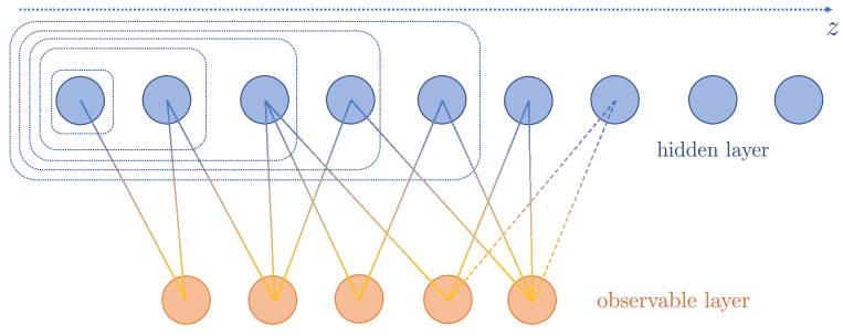
Figure 1: The concept of the grand-canonical extension to the rbm. Hidden units are ordered from left to right into layers of different lengths $z$ (dashed rectangles). Each hidden layer is proportionally penalized according to $z$ by a chemical potential which is dynamically determined during training. Provided an observable distribution hidden layers of the appropriate size are invoked to model the target data.

In practice, we have to impose a cutoff to the maximal size of hidden layers that the grand-canonical model could use. For a sufficiently high cutoff though, not only we anticipate that the theory effectively becomes independent of the concrete cutoff implemented, but furthermore that most designer choices concerning the precise functional form of the chemical potential converge to the same regularizing effect.

The method of regularization presented in this paper fundamentally differs from the familiar $\ell_{p}$ – regularization w.r.t. two aspects. On the one hand, once the chemical potential is appropriately chosen as a function of the rest of the rbm parameters, there should remain no adjustable parameter – discrete or continuous – related to the strength of regularization. On the other side, this regularization scheme naturally treats target data in a local fashion. This means that networks with a different number of hidden units will be invoked for different subsets of the target data depending on concrete features of each subset. In the language of mathematical optimization, training an rbm under standard $\ell_{p}$ – regularization poses a hardly constrained problem, while training the suggested grand-canonical extension with an appropriately chosen chemical potential results into a softly constrained problem.

Overview of the paper

This paper is structured into a theoretical (Section 2) and applied (Section 3) part. Specifically, we review in Section 2.1 the necessary theoretical framework of grand-canonical Boltzmann distributions and lay out the model we wish to investigate. Subsequently, we set up in Section 2.2 the stage for training, by revisiting the minimization of the cross entropy between target and model distribution, while explaining necessary modifications at the level of a numerical solution. Next, we discuss in Section 2.3 working assumptions and justify our concrete choice of the chemical potential as a function of the weights and biases that penalizes larger hidden layers. Ultimately, we apply the developed techniques to two well-known data sets: two-dimensional Ising configurations and the mnist set of handwritten digits, in Sections 3.1 and 3.2, respectively. We discuss and compare the learning outcome among the two paradigms as well as to the standard rbm (without regularization).

2 Varying number of hidden units

A restricted (i.e. in absence of intra-layer interactions) Boltzmann machine consists of an observable layer with $N$ units $\textbf{v}\equiv\{v^{i}\}_{i=1,...,N}$ and a hidden layer with $z$ units $\textbf{h}^{z}\equiv\{h^{a}\}_{a=1,...,z}$. In this picture, the observed interactions among the units v are modelled via their connection to the hidden (or latent) units $\textbf{h}^{z}$. Generically, Boltzmann machines are characterized by the weights (also called connections) $\omega_{ai}$ among observable and hidden layer together with the hidden and observable biases, $\beta_{a}$ and $\xi_{i}$ respectively. In the following, we collectively denote the trainable rbm parameters by $\lambda\equiv\{\omega_{ai},\beta_{a},\xi_{i}\}$. In contrast to those parameters which are expected to be fixed during training by extremizing the appropriate information-theoretic metric, the number of hidden units $z$ is a so-called hyperparameter which needs to be fine-tuned beforehand.

In what follows, the question we are going to answer is how to eliminate this hyperparameter from training or in other words, leaving the size of the hidden layer unconstrained if and how the machine can “select” by itself optimum values for $z$ to explain the provided data. For brevity, we shall refer to a restricted Boltzmann machine invoking a varying number of hidden units as vrbm.

2.1 Boltzmann machine at finite chemical potential

Henceforth, we focus for concreteness on a binary domain where $v^{i}=\pm 1$ and Bernoulli Boltzmann machines also with $h^{a}=\pm 1$; the generalization of our discussion to Gaussian or other multimodal models being straight-forward. As we are interested to work in this paper with varying number of hidden units $z\in\mathbb{N}$, we need to switch to the grand-canonical ensemble. In this picture, the proper energy-based model at finite chemical potential $\mu$ is given by the grand-canonical Boltzmann distribution

$$p(\textbf{v},\textbf{h}^{z},z)=\frac{1}{Z}{\text{e}}^{-E-\mu\,z}\quad\text{with}\quad E\equiv E(\textbf{v},\textbf{h}^{z},z)=-\sum_{a=1}^{z}\sum_{i=1}^{N}h^{a}\omega_{ai}v^{i}-\sum_{a=1}^{z}h^{a}\beta_{a}-\sum_{i=1}^{N}\xi_{i}v^{i}~{},$$ (2.1)

$Z$ being the (generally intractable) partition function. Indices are contracted in Euclidean space and summations are explicitly recorded, for clarity. We work in units where $[k_{B}T]=1$. Including terms up to quadratic order in the units $v^{i}$ and $h^{a}$ helps efficiently solve the extremization problem posed during training, as outlined in Section 2.2. Setting $\mu=0$ in Eq. (2.1) recovers the ordinary rbm dictated by the canonical Boltzmann distribution.

Introducing the shorthand notations

$$\sum_{\textbf{v}}\equiv\prod_{i=1}^{N}\sum_{v_{i}}\quad\text{and}\quad\sum_{\textbf{h}^{z}}\equiv\prod_{a=1}^{z}\sum_{h_{a}}$$ (2.2)

it is useful to define the free energies in the grand-canonical ensemble for a hidden layer of length $z$ via

$$F_{\lambda,\mu}(\textbf{v},z)= \,\,\mu\,z-\sum_{i=1}^{N}\xi_{i}\,v^{i}-z\log 2-\sum_{a=1}^{z}\log\cosh\left(\sum_{i=1}^{N}\omega_{ai}\,v^{i}+\beta_{a}\right)$$ (2.3)

$$\text{and}\quad F_{\lambda,\mu}(\textbf{h}^{z},z)= \,\,\mu\,z-\sum_{a=1}^{z}h^{a}\beta_{a}-N\log 2-\sum_{i=1}^{N}\log\cosh\left(\sum_{a=1}^{z}h^{a}\,\omega_{ai}+\xi_{i}\right)$$ (2.4)

by integrating out hidden and observable variables, respectively. $z$-independent terms like $N\log 2$ can be dropped. At most, we can absorb an irrelevant for our purposes (since it leads to a $z$-suppression irrespective of the training procedure) term like $z\log 2$ by redefining the chemical potential. Integrating out the hidden variables and summing over all possible lengths $z$ of the hidden layer leads to the observable free energy of the vrbm,

$$F_{\lambda,\mu}(\textbf{v})=-\log\sum_{z=1}^{\infty}{\text{e}}^{-F_{\lambda,\mu}(\textbf{v},z)}=-\sum_{i=1}^{N}\xi_{i}v^{i}-\log\left[\sum_{z=1}^{\infty}{\text{e}}^{-\mu\,z}\prod_{a=1}^{z}2\cosh\left(\sum_{i=1}^{N}\omega_{ai}\,v^{i}+\beta_{a}\right)\right]~{},$$ (2.5)

in terms of which the partition function of the model compactly reads

$$Z\equiv Z(\lambda,\mu)=\sum_{\textbf{v}}{\text{e}}^{-F_{\lambda,\mu}(\textbf{v})}~{}.$$ (2.6)

Evidently, the associated probabilities we are going to use in the following section are generically given by

$$p_{\lambda,\mu}(\textbf{v})=\frac{1}{Z}e^{-F_{\lambda,\mu}(\textbf{v})}\quad\text{and}\quad p(\textbf{v},z)=\frac{1}{Z}e^{-F_{\lambda,\mu}(\textbf{v},z)}~{}.$$ (2.7)

At this stage, the partition function $Z$ of the vrbm depends on the ordinary rbm parameters $\lambda$ as well as the chemical potential $\mu$. This model can be viewed as a collection of ordinary Boltzmann machines with a hidden layer of different lengths $z$. Hence, rbm with different number of hidden units contribute to grand-canonical expectation values weighted by the introduced chemical-potential term. From the point of view of statistical systems, our vrbm is expected to exhibit different phases: For $\mu\gg 1$ smaller hidden layers are favoured prohibiting learning the desired distribution, while in the opposite limit networks with larger number of hidden units prevail and overfitting occurs.

Working assumptions.

For the intended ml application, we can only sum over a finite number $K$ of sizes $z$ of the hidden layer. We thus have to use the free energy

$$F_{\lambda,\mu,K}(\textbf{v})=-\log\sum_{z=1}^{K}{\text{e}}^{-F_{\lambda,\mu}(\textbf{v},z)}~{},$$ (2.8)

whose limiting case is Eq. (2.5). This model has one more parameter than the partition function Eq. (2.6) of the idealized vrbm: the maximum number $K$ of hidden units that the model has at its disposal. In the spirit of eliminating hyperparameters and assuming that only a finite number of hidden units is needed to explain the target data, we take the number of available hidden units to be very large until the model “thinks” it always has a sufficient number of resources. Formally, we shall work in the regime of large $K$. To quantify this, $K$ needs to be sufficiently larger than the natural scale of the problem set by the number of observable units $N$, so that effects induced by the finite amount of hidden resources are suppressed by powers of $N/K\ll 1$. In the following, we shall always work in the approximation $F_{\lambda,\mu,K\gg N}(\textbf{v})\approx F_{\lambda,\mu}(\textbf{v})$. In practice, as we are going to see in Section 3 this can be relaxed to $K>N$.

Even under the large-$K$ regime, the model described by partition function Eq. (2.6) still seems to have annoyingly many adjustable parameters, for sure not less than its canonical counterpart. Most crucially, we are not interested to merely swap the discrete number $z$ of hidden units with a continuous chemical potential $\mu$, but to eliminate the hyper-parameter determining the size of the hidden layer from the training altogether. Hence, we shall take the chemical potential to be some function of the other rbm parameters, $\mu\equiv\mu(\lambda)$. Generically, there are a few desired properties this function is expected to possess. First of all, at the formal level, the chemical potential being an intensive variable will be treated as a global model parameter, i.e. it will not exhibit any explicit or implicit dependance on the hidden-layer number $z$. At the practical level, dropping this constraint leads to certain instabilities in the learning process, at least for the systems tested in this work. In addition, to ensure that $\mu$ has a regularizing effect at all, it should be independent from the sign of the other parameters, weights $\omega$ and biases $\beta$. Given those formal requirements one is entitled to test which ansatz for $\mu$ best suits the training on a particular target system.

For the purposes of this paper, we adopt a full agnostic approach concerning the target system and refrain from imposing any designer biases. Specifically, as the biases $\xi_{i}$ solely characterize observable units, the chemical potential $\mu$ – being a feature that is intimately related to the length of the hidden layer – is not expected to explicitly depend upon those. In the same spirit, we further assume that $\mu$ is unbiased towards observable units, i.e. it does not exhibit any implicit dependance on them, as well. Thus, our chemical potential is at most a function of the row p-norm of the weight matrix and hidden biases,

$$\mu\equiv\mu\left(\sum_{i=1}^{N}\left|\omega_{ai}\right|^{p},\beta_{a}\right)~{}.$$ (2.9)

In what follows, we take all model quantities to ultimately depend only on the trainable parameters $\lambda$ that are determined by appropriate training, as outlined in the next paragraph.

The extremization condition.

A generative model is primarily used to learn to reproduce a given data distribution $q(\textbf{v})$ by extracting its characteristic features. In the following, we always take the domain of $q(\textbf{v})$ to coincide with the domain of both the observable and hidden units of our generative model. Training our Boltzmann machine on a given target probability $q(\textbf{v})$ is performed by extremizing w.r.t. model parameters $\lambda$ (recall that we take $\mu\equiv\mu(\lambda)$) an appropriately chosen target function. As a target function we conventionally take the opposite of the cross entropy between model and target distribution, i.e. the expectation value under target distribution $q(\textbf{v})$ of the logarithm of probability $p_{\lambda}(\textbf{v})$ given in Eq. (2.7):

$$t(\lambda)\equiv\sum_{\textbf{v}}q(\textbf{v})\log p_{\lambda}(\textbf{v})~{}.$$ (2.10)

It is straight-forward to show that maximizing $t(\lambda)$ is equivalent to minimizing the Kullback-Leibler divergence which gives the relative entropy between target $q(\textbf{v})$ and model $p_{\lambda}(\textbf{v})$ distribution.

First, note that deriving free energy Eq. (2.5) w.r.t. some trainable parameter $\lambda$ we get

$$\frac{\partial}{\partial\lambda}F_{\lambda}(\textbf{v})=\sum_{z=1}^{K}p_{\lambda}\left(z|\textbf{v}\right)\frac{\partial F_{\lambda}(\textbf{v},z)}{\partial\lambda}~{},$$ (2.11)

where the conditional probability associated to Eq. (2.3) reads

$$p_{\lambda}\left(z|\textbf{v}\right)=\frac{p_{\lambda}\left(\textbf{v},z\right)}{p_{\lambda}\left(\textbf{v}\right)}=\frac{{\text{e}}^{-F_{\lambda}(\textbf{v},z)}}{{\text{e}}^{-F_{\lambda}(\textbf{v})}}=\frac{e^{-\mu z}\prod_{a=1}^{z}2\cosh\left(\sum_{i=1}^{N}\omega_{ai}\,v^{i}+\beta_{a}\right)}{\sum_{z^{\prime}=1}^{K}e^{-\mu z^{\prime}}\prod_{a^{\prime}=1}^{z^{\prime}}2\cosh\left(\sum_{i^{\prime}=1}^{N}\omega_{a^{\prime}i^{\prime}}\,v^{i^{\prime}}+\beta_{a^{\prime}}\right)}~{}.$$ (2.12)

Next, we can express the extremization condition on $t(\lambda)$ in terms of a derivative of the free energy Eq. (2.3) at level $z$:

$$0\overset{!}{=}\frac{\partial}{\partial\lambda}t(\lambda)= \,\,\sum_{\textbf{v}}\sum_{z=1}^{K}\left[q\left(\textbf{v}\right)p_{\lambda}\left(z|\textbf{v}\right)-p_{\lambda}\left(\textbf{v},z\right)\right]\frac{\partial(-F_{\lambda}(\textbf{v},z))}{\partial\lambda}~{}.$$ (2.13)

Using the concrete form (2.1) of grand-canonical Boltzmann distribution the extremization condition (2.13) results into a set of $(K\times N+K+N)$ equations,

$$\sum_{\textbf{v}} \sum_{z=1}^{K}\left\{H(z-a)\tanh\left(\sum_{i^{\prime}=1}^{N}\omega_{ai^{\prime}}v^{i^{\prime}}+\beta_{a}\right)v^{i}-\frac{\partial\mu}{\omega_{ai}}\,z\right\}\left[q\left(\textbf{v}\right)p_{\lambda}\left(z|\textbf{v}\right)-p_{\lambda}\left(\textbf{v},z\right)\right]=0$$

$$\sum_{\textbf{v}} \sum_{z=1}^{K}\left\{H(z-a)\tanh\left(\sum_{i^{\prime}=1}^{N}\omega_{ai^{\prime}}v^{i^{\prime}}+\beta_{a}\right)-\frac{\partial\mu}{\beta_{a}}\,z\right\}\left[q\left(\textbf{v}\right)p_{\lambda}\left(z|\textbf{v}\right)-p_{\lambda}\left(\textbf{v},z\right)\right]=0$$

$$\sum_{\textbf{v}} v^{i}\left[q\left(\textbf{v}\right)-p_{\lambda}\left(\textbf{v}\right)\right]=0~{},$$ (2.14)

taking $\lambda=\omega_{ai},\beta_{a},\xi_{i}$ respectively. Notice in particular, the appearance of Heaviside step function $H$ with $H(x)=1$ for $x\geq 0$, as a consequence of varying number of hidden units as well as the additional term in the first two equations due to the derivative of chemical potential Eq. (2.9).

In the literature, such extremization conditions are often compactly written as

$$\left\langle h^{a}v^{i}\right\rangle_{\text{data}}-\left\langle h^{a}v^{i}\right\rangle_{\text{model}}-\frac{\partial\mu}{\omega_{ai}}\left(\langle z\rangle_{\text{data}}-\langle z\rangle_{\text{model}}\right)= \,\,0$$

$$\langle h^{a}\rangle_{\text{data}}-\langle h^{a}\rangle_{\text{model}}-\frac{\partial\mu}{\beta_{a}}\left(\langle z\rangle_{\text{data}}-\langle z\rangle_{\text{model}}\right)= \,\,0$$

$$\langle v^{i}\rangle_{\text{data}}-\langle v^{i}\rangle_{\text{model}}= \,\,0~{},$$ (2.15)

where expectation values are understood to be taken w.r.t. the distribution of the provided training data $q(\textbf{v})$ and the probability distribution $p_{\lambda}(\textbf{v})$ generated by our model. Due to our inability to generically evaluate the partition function $Z(\lambda)$ the derived set of conditions cannot be solved in any closed form.

2.2 Contrastive Divergence revisited.

To circumvent this we shall make a gradient-descend inspired approximation. Employing contrastive divergence (cd) has proven to be a particularly efficient way to numerically find the maximum, Eq. (2.13), by updating our model parameters $\lambda$ in the direction of steepest descend according to

$$\lambda^{(\alpha+1)}=\lambda^{(\alpha)}+\gamma\,\nabla_{\lambda}^{(\alpha)}\langle\log p(\textbf{v})\rangle_{\text{data}}$$ (2.16)

until convergence is achieved. The learning rate $\gamma$ is a tuneable parameter of the extremization process itself. Too large values of $\gamma$ could drive away from the desired extremum, while too small learning rates slow down the training process. The cd derivative at $\alpha$-th step is defined by

$$\nabla_{\lambda}^{(\alpha)}\equiv\beta\,\nabla_{\lambda}^{(\alpha-1)}+\left(1-\beta\right)\frac{\partial}{\partial\lambda^{(\alpha)}}~{},$$ (2.17)

where $\alpha=0,1,...$ with $\nabla_{\lambda}^{(-1)}=0$. The momentum $\beta\in[0,1)$ acts as a “memory” of previous updates to ensure stability of the gradient-descent algorithm.

The mean-field ansatz.

For each cd update in Eq. (2.16) we need to compute the expectation values in Eq. (2.1) that appear when taking the derivative of the target function $t(\lambda)$ w.r.t. model parameters $\omega_{ai}$, $\beta_{a}$ and $\xi_{i}$. For that, we use mean-field theory to iteratively compute the vev of $v^{i}$, $h^{a}$ and $z$ using consistency equations and substituting the one into the other. In our vrbm setting though, a slight modification of the mean-field theoretic consistency conditions which are invoked by the cd method in the standard rbm construction is required. Schematically, starting from the distribution v of observable units the length of hidden layer $z$ and subsequently the hidden units $\textbf{h}^{z}$ are to be inferred which in turn are about to give a new estimation for v.

In detail, provided the distribution of observable units $q(\textbf{v})$ it is straight-forward to compute the multimodal conditional probability $p(z|\textbf{v})$ given in Eq. (2.12). As in ordinary Boltzmann machines, we calculate the expectation value of the hidden units provided a sample v from the observable distribution from the (grand-canonical in our case) free energy Eq. (2.5) by

$$\langle h^{a}\rangle_{\textbf{v}}=\frac{\partial}{\partial\beta_{a}}\left(-F(\textbf{v})\right)=\sum_{z=1}^{K}\frac{\partial(-F(\textbf{v},z))}{\partial\beta_{a}}p(z|\textbf{v})=P(z\geq a|\textbf{v})\tanh\left(\sum_{i=1}^{N}\omega_{ai}\,v^{i}+\beta_{a}\right)$$ (2.18)

using Eq. (2.11). The complementary cumulative distribution function (ccdf) or survival function of the probability $p(z|\textbf{v})$,

$$P(z\geq a|\textbf{v})\equiv\sum_{z=a}^{K}p(z|\textbf{v})~{},$$ (2.19)

ensures that only layers including the $a$-th hidden unit contribute to its conditional expectation value, cf. Eq. (2.1). Next, we need to determine some optimum value for the size of the hidden layer $z$ being sufficient to extract the features from the provided observable distribution. In principle, the number $z$ of hidden units has to be determined by sampling from $p(z|\textbf{v})$. In practice, it is computationally cheaper while converging faster to either compute the vev of $z$ provided v,

$$\langle z\rangle_{\textbf{v}}=\sum_{z=1}^{K}z\,p(z|\textbf{v})~{},$$ (2.20)

and round it upwards to the nearest integer, or take the largest most probable value for $z$ given its conditional distribution,

$$z_{\text{probable}}=\max\left\{z~{}|~{}\max_{z}\,p(z|\textbf{v})\right\}~{}.$$ (2.21)

After sufficient number of training epochs and at large $K$, all methods effectively lead to the same outcome. Ultimately, given the derived value of $z$ together with $\langle h^{a}\rangle_{\textbf{v}}$ we are in a position to deduce a new estimation for $v^{i}$. Such an estimation has to be extracted from a Boltzmann machine with $z$ hidden units taking values $\langle h^{a}\rangle_{\textbf{v}}$ via

$$\langle v^{i}\rangle_{\textbf{h}^{z},z}=\frac{\partial(-F(\textbf{h}^{z},z))}{\partial\xi_{i}}=\sum_{v^{i}}v^{i}\,p(v^{i}|\textbf{h}^{z},z)=\tanh\left(\sum_{a=1}^{z}h^{a}\omega_{ai}+\xi_{i}\right)~{},$$ (2.22)

where the necessary conditional probability is deduced from Eq. (2.4),

$$p(v^{i}|\textbf{h}^{z},z)=\frac{p(v^{i},\textbf{h}^{z},z)}{p(\textbf{h}^{z},z)}=\frac{{\text{e}}^{-E(v^{i},\textbf{h}^{z},z)-\mu z}}{{\text{e}}^{-F(\textbf{h}^{z},z)}}=\frac{{\text{e}}^{\left(\sum_{a=1}^{z}h^{a}\omega_{ai}+\xi_{i}\right)v^{i}}}{2\cosh\left(\sum_{a=1}^{z}h^{a}\omega_{ai}+\xi_{i}\right)}~{}.$$ (2.23)

Hence, $z$ hidden units contribute to the feature extraction from the desired data set leading in turn, to the generation of a new estimation for $\{v_{i}\}$. As our estimation for $z$, either Eq. (2.20) or Eq. (2.21), depends on the initial configuration v that we sample from input distribution $q(\textbf{v})$, we observe that different configurations from $q(\textbf{v})$ would generically be explained by a different number of hidden units. In other words, the vrbm model has the freedom to adjust the size $z$ of its hidden layer depending on the complexity level of each subset in $q(\textbf{v})$. This observation constitutes one of the fundamental departures from standard $\ell_{p}$ – regularization [40] (the other main difference being the absence of a continuous parameter conventionally controlling the strength of ordinary regularization schemes). When regularization is globally applied to the input set $q(\textbf{v})$ the local features of each example configuration v are detected by the same fixed number of hidden units encompassing the danger of over-learning for some of the subsets in $q(\textbf{v})$.

In total, the $k$-th iteration in mean-field theory for $k\in\mathbb{N}$ reads

$$z_{(k-1)}\equiv\langle z\rangle_{\textbf{v}^{(k-1)}}~{}\text{ and }~{}h^{a}_{(k-1)}\equiv\langle h^{a}\rangle_{\textbf{v}^{(k-1)}}\quad\longrightarrow\quad v^{i}_{(k)}\equiv\langle v^{i}\rangle_{\textbf{h}^{(k-1)},\,z^{(k-1)}}~{},$$ (2.24)

under the initial configuration $v^{i}_{(0)}\equiv v^{i}$ described by $q(\textbf{v})$. For well-defined extrema, mean-field theory is formally expected to converge towards $\langle v^{i}\rangle$, the very latest as $k\rightarrow\infty$. In practice, the mean-field ansatz converges for physical data beyond numerical accuracy already when $k=2$.

Summary of the numerical method.

All in all, putting everything together the $\alpha$-th step of the cd method in the vrbm dictated by Eq. (2.16) under a mean-field theoretic ansatz after $k$ steps in Eq. (2.24) consists of

$$\omega^{(\alpha+1)}_{ai}= \,\,\omega^{(\alpha)}_{ai}+\gamma\left\{\beta+\left(1-\beta\right)\delta_{ab}\,\delta_{ij}\left[{h^{b}_{(0)}}{v^{j}_{(0)}}-{h^{b}_{(k)}}{v^{j}_{(k)}}-\frac{\partial\mu}{\partial\omega^{(\alpha)}_{bj}}\left(z_{(0)}-z_{(k)}\right)\right]\right\}$$

$$\beta^{(\alpha+1)}_{a}= \,\,b^{(\alpha)}_{a\phantom{ii}}+\gamma\left\{\beta+\left(1-\beta\right)\delta_{ab}\left[{h^{b}_{(0)}}-{h^{b}_{(k)}}-\frac{\partial\mu}{\partial\beta_{b}^{(\alpha)}}\left(z_{(0)}-z_{(k)}\right)\right]\right\}$$

$$\xi^{(\alpha+1)}_{i}= \,\,\xi^{(\alpha)}_{i\phantom{ai}}+\gamma\left\{\beta+\left(1-\beta\right)\delta_{ij}\left[{v^{j}_{(0)}}-{v^{j}_{(k)}}\right]\right\}~{}.$$ (2.25)

Kronecker delta is used to raise and lower indices. Compared to the standard rbm its grand-canonical extension adds a complexity in computing conditional probability Eq. (2.12) which grows linearly in the maximum number of hidden units $K$ the model has at its disposal, cf. Eq. (2.8). Apart from computing this multimodal distribution, the grand-canonical cd algorithm shares everything with its canonical counterpart. Setting $\mu=0$ in the equations (2.2) and taking $p(z|\textbf{v})=\delta_{z,z_{0}}$ in Eq. (2.18) – (2.23) reproduces the ordinary cd algorithm of the rbm in the canonical ensemble with fixed number $z_{0}$ of hidden units.

2.3 A penalizing chemical potential

So far, we have avoided to concretely specify the form of the chemical potential, besides a more generic discussion towards the end of Section 2.1. In particular, we have explained our motivation in taking $\mu\equiv\mu(\lambda)$ and discussed about the anticipated functional form of $\mu>0$ concluding to Eq. (2.9) in order to regulate the length of the hidden layer. Of course, being an intensive quantity $\mu$ could well implicitly or explicitly depend on global non-trainable parameters like $N$ and $K$, but not on $z$ itself.

Given that the additional term in the grand-canonical ensemble is expected to naturally act as a regularizer for the number of hidden units and by naive dimensional analysis, the chemical potential should have the form of a non-negative energy density:

$$\mu=\frac{\text{non-negative ``vacuum energy''}}{\text{number of active hidden units}}~{},$$ (2.26)

where the number of active hidden units equals the number of $h^{a}$ participating in explaining the target data, i.e. have non-vanishing weights $\omega_{ai}$ for at least one $i$. Conceptually, our ansatz (2.26) for the chemical potential describes some notion of total non-negative – to achieve a regularizing effect – vacuum energy (which could well be infinite when $K\rightarrow\infty$) that is equally partitioned over each hidden unit actively participating in extracting the features of the target data. That way, we uniformly define a penalty the model needs to pay for using additional hidden units. Networks with larger hidden layers are then proportionally penalized to their length $z$ by a factor $\mu$ that equals the aforementioned “vacuum-energy” density.

Even under the working assumptions of paragraph 2.1, there is still a certain freedom in specifying the form of the total “vacuum energy” in Eq. (2.26). Inspired mainly from the regularization procedure performed [32, 41] in ordinary rbm it seems plausible to take as a definition of the “vacuum energy” entering the chemical potential,

$$\text{non-negative ``vacuum energy''}=\sum_{a=1}^{K}\mathcal{E}_{a}~{},$$ (2.27)

introducing the fundamental “vacuum-energy” quantum

$$\mathcal{E}_{a}=\mbox{$\frac{1}{N}$}\sum_{i=1}^{N}\left|\omega_{ai}\right|^{p}+\left|\beta_{a}\right|^{p}$$ (2.28)

characterizing each hidden unit. Notice that $\mathcal{E}_{a}$ depends on the $a$-th row $p$ – norm of the weight matrix and the respective hidden bias. In a similar spirit, the matrix norm of $\omega$ appearing in definition (2.27) avoids placing any bias over some specific observable $v^{i}$ or hidden $h^{a}$ unit that could falsify a fair learning of the necessary connections $\omega_{ai}$.

Concerning the denominator of Eq. (2.26) that should count the number of hidden units actively used by the vrbm to model the given data it is straight-forward to approximate it by a smooth (since $\tanh\mathcal{E}_{a}\rightarrow 1$ asymptotically when $\mathcal{E}_{a}\gg 1$) counter,

$$K_{\text{eff}}=\text{number of active hidden units}\approx\sum_{a=1}^{K}\tanh\mathcal{E}^{a}~{}.$$ (2.29)

In fact, to precisely count the number of active units we would have to replace $\tanh$ by ReLu function. However, the infinitely steep derivative of the latter function when its argument becomes zero renders the numerical solution presented in Section 2.2 inadequate, as the cd method gets stack either to the $\mu\approx 0$ regime or $\mu\gg 1$ depending on initial conditions. Hence in total, a candidate chemical potential depending only on the row-norm of $\omega$ and hidden biases $\beta$ which is unbiased towards any hidden or observable unit reads

$$\mu\equiv\mu(\omega,\beta)=\frac{\sum_{a=1}^{K}\left(\mbox{$\frac{1}{N}$}\sum_{i=1}^{N}\left|\omega_{ai}\right|^{p}+\left|\beta_{a}\right|^{p}\right)}{\sum_{a^{\prime}=1}^{K}\tanh\left(\mbox{$\frac{1}{N}$}\sum_{i^{\prime}=1}^{N}\left|\omega_{a^{\prime}i^{\prime}}\right|^{p}+\left|\beta_{a^{\prime}}\right|^{p}\right)}\,\equiv\,\frac{\sum_{a=1}^{K}\mathcal{E}_{a}}{\sum_{a^{\prime}=1}^{K}\tanh\mathcal{E}_{a^{\prime}}}~{}.$$ (2.30)

Alternatively, depending on the input data to ensure numerical stability one could further smoothen this definition by taking the $\cosh$ of Eq. (2.27).

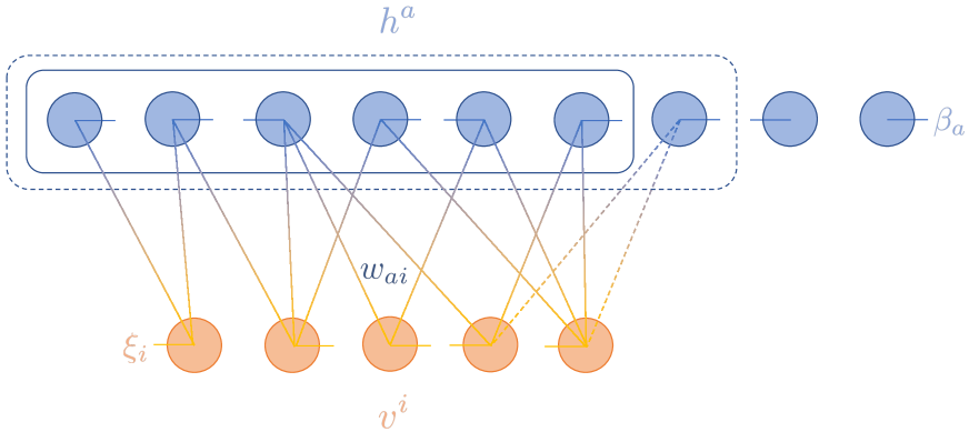
Figure 2: In the self-regularizing rbm the interactions among observable units $v^{i}$ with biases $\xi_{i}$ are modelled by connecting via weights $w_{ai}$ to hidden units $h^{a}$. To explain an observable configuration some of the hidden units might not be used in spite of having weights (dashed lines) which have been trained on the full data set. Additionally, there are hidden units which do not participate in feature extraction, at all, while their biases $\beta_{a}$ still contribute to the regularization procedure.

At this point, a few remarks are in order: Evidently, our energy quantum $\mathcal{E}_{a}\geq 0$ is solely controlled by the respective bias, when the hidden unit is inactive in the sense of $\omega_{ai}=0$ for all $i=1,..,N$. Consequently, the model has the ability to recursively adjust $K_{\text{eff}}$ and $\mu$ by merely administrating the hidden biases $\beta_{c}$ (and hence $\mathcal{E}_{c}$) of the latter $(K-K_{\text{eff}})$ inactive units $h^{c}$ without interfering much with the actual training of the first $K_{\text{eff}}$ units $h^{b}$. To control the aforementioned interference between regularization and learning those first $h^{b}$ units the $b$-th row $p$-norm of the weight-matrix $\omega$ entering definition (2.28) was normalized by the observable scale $N$. For finite values of $K$, this seems to be the most sensible normalization in order to avoid naively introducing any hierarchy in $N$ among the two summands in Eq. (2.28). At large $K$ (i.e. $K\gg N$) however, we anticipate (and indeed find) that any generic number in front of $\left|\omega_{ai}\right|$ leads to the same outcome after sufficient number of epochs. The same observation holds for any generic rescaling of the hidden biases entering Eq. (2.28). Despite that such redefinitions of the chemical potential could delay the convergence of the training algorithm, they do not crucially change the regularizing effect of Eq. (2.30) which is determined by our conceptual choice of the functional form Eq. (2.26).

In Figure 2, we schematically draw how the vrbm is expected to model interactions among five observable units $v^{i}$ by using their connection (continuous lines) to hidden units $h^{b}$ via the trained weights $w_{bi}$. Not all weights that the vrbm has learned during training are expected to participate in the feature detection of each example from the target distribution $q(\textbf{v})$. In our schematic depiction, one hidden unit remains inactive (dashed connecting lines) for the given observable configuration v as dictated by $p(z|\textbf{v})$. The size of the biggest hidden network (wrapped by a dashed rectangular) encompassing all units $h^{b}$ connecting to the observable layer determines $K_{\text{eff}}$. Finally, there should exist hidden units $h^{c}$ for $c>K_{\text{eff}}$ whose weights are effectively regularized to zero. In fact, weights $w_{ci}$ with $c>K_{\text{eff}}$ quickly get exponentially suppressed by the chemical-potential term in $p(z|\textbf{v})$ beyond any meaningful numerical accuracy. The role of those hidden units is to ensure the regularizing effect of the vrbm through their biases $\beta_{c}$, as we are going to explicitly verify in the following two sections.

To summarize, the grand-canonical extension of the rbm is expected to dynamically determine during training the most optimal value of a penalizing chemical potential $\mu$ in order to extract the typical characteristics of the target distribution at a satisfactory level while avoiding over-learning. To do so, it employs –  provided a sufficiently large number of hidden units – hidden layers of different lengths $z$ depending on the input configuration v with a probability $p(z|\textbf{v})$.

3 Training Boltzmann machines at finite chemical potential

In this section, we aim at applying the grand-canonical extension of the rbm developed in the previous paragraphs to learn target distributions $q(\textbf{v})$ that act as a reference in their respective fields. For this purpose, two error functions which measure the deviation of the ml-generated data from the actual data set come in handy. So far, the prediction of our model derived in Section 2.2 is an expectation value $\langle v^{i}\rangle$ of the mean-field theoretic ansatz Eq. (2.24) for each observable unit. A priori, $\langle v^{i}\rangle$ is not expected to belong to the domain of $q(\textbf{v})$, though. As those error measures are concerned with the crucial ability of the generative model to learn and reproduce the target data, one should stochastically replace the expectation value $\langle v^{i}\rangle$ with the actual value $v^{i}$ as sampled from distribution (2.23). For binary distributions, given the expectation value that is computationally more efficient to obtain, this replacement is simply done with a probability $P(v^{i}=\pm 1)=(1\pm\langle v^{i}\rangle)/{2}$.

Loss functions.

In most applications of interest, training the ml model on the full distribution $q(\textbf{v})$, which is usually not fully known or very expensive to compute, is not a feasible task. In practice, we train our generative model on a smaller number of $\mathcal{N}_{\text{train}}$ selected points $\textbf{v}_{A}=\{v_{A}^{i}\}_{i=1,...,N}$ sampled from $q(\textbf{v})$. For ease of notation, we summarize the training subset via

$$q_{\text{train}}(\textbf{v})\equiv\frac{1}{\mathcal{N}_{\text{train}}}\sum_{A}\prod_{i=1}^{N}\delta(v^{i}-v^{i}_{A})~{},$$ (3.31)

in terms of one-dimensional delta functions (or Kronecker delta for discrete distributions). To express the ability of the generative model to accurately learn to reproduce $q_{\text{train}}(\textbf{v})$ we introduce the quadratic reconstruction error on training data (also called train loss function) by

$$\varepsilon_{\text{train}}:=\sum_{\textbf{v}}q_{\text{train}}(\textbf{v})\sum_{i=1}^{N}\left(v^{i}-\langle v^{i}\rangle\right)^{2}~{}.$$ (3.32)

For the expectation value we substitute the prediction $\textbf{v}^{(k)}$ of our model after $k$ steps in mean-field theory according to Eq. (2.24) to closely follow the convergence of our algorithms. To benchmark the quality of learning, i.e. to which extend our generative model has correctly identified important features of the target distribution to faithfully reconstruct new – unseen during training – data points $\textbf{v}_{B}=\{v_{B}^{i}\}_{i=1,...,N}$ from $q(\textbf{v})$, summarized by

$$q_{\text{test}}(\textbf{v})\equiv\frac{1}{\mathcal{N}_{\text{test}}}\sum_{B}\prod_{i=1}^{N}\delta\left(v^{i}-v^{i}_{B}\right)~{},$$ (3.33)

we invoke the quadratic reconstruction error on test data (or test loss function)

$$\varepsilon_{\text{test}}:=\sum_{\textbf{v}}q_{\text{test}}(\textbf{v})\sum_{i=1}^{N}\left(v^{i}-\langle v^{i}\rangle\right)^{2}~{}.$$ (3.34)

Also here, we substitute our estimation $\textbf{v}^{(k)}$ of the expectation value deduced by iteratively applying Eq. (2.24) during training to monitor the learning quality.

In the same spirit, one could define absolute learning errors by taking the absolute value of the difference between target data and mean-field theoretic outcome. This makes sense especially for continuous distributions (where the quadratic loss function could underestimate the learning error in the domain $[0,1]$) or when outliers in the training data being overweighted by the quadratic loss erroneously lead to big training but still reasonable test errors. Evidently, $\varepsilon_{\text{train}}\rightarrow 0$ means that our ml algorithm is able to accurately reproduce the provided points from target distribution $q(\textbf{v})$, while $\varepsilon_{\text{test}}\rightarrow 0$ signifies the ability of our model to generalize into unseen data after correctly extracting the characteristic traits of $q(\textbf{v})$ during training.

At first sight, the outlined way to use these loss functions seems to depart from their general objective, as described in the beginning, which is to judge the actual prediction on the domain of the generative model (i.e. the integer value $v^{i}$ for discrete distributions). However, after a sufficient number of epochs for the binary systems under consideration, we observe that $\langle v^{i}\rangle$ indeed converges towards the domain values $\pm 1$. Consequently the probability $P(v^{i}=\pm 1)$ to find the $i$-th unit with value $\pm 1$ sharply peaks at 0 or 1 depending on the expectation value $\langle v^{i}\rangle$. In turn, this signals that $\langle v^{i}\rangle$ effectively coincides with the sampled value $v^{i}$ within the domain of our model. For this reason, after a desired accuracy has been achieved, it is allowed to simply round $\langle v^{i}\rangle$ to the nearest integer. As we are primarily interested in this work in benchmarking the convergence rate and learning quality of the formally developed grand-canonical extension to the rbm, we shall not further discuss sampling options and evaluate the loss functions on the mean-field theoretic ansatz.

Computational simplications.

In developing the theoretical framework for the vrbm we have been appealing to the large order of hidden units, $K\gg N$, to render certain designer choices in the form of the chemical potential equivalent. The regime of large $K$ is a key feature to ensure the desired elimination of the length of the hidden layer as a hyperparameter. One might wonder whether such a regime is in practice feasible, beyond a mere theoretical playground. On the one hand, it turns out that $K$ does not need to be that large for the vrbm to work in a satisfactory self-regularizing manner. At least for the systems we have considered, finite-$K$ effects appear way beyond $\varepsilon_{\text{test}}$, for very reasonable values of $K$, not influencing thus the quality of learning. On the other hand, larger networks become quickly – already from the first cd steps – exponentially suppressed in $p(z|\textbf{v})$, thus setting hidden expectation values $\langle h^{a}\rangle$ for larger $a$ effectively to zero (see Eq. (2.18)). Hence, one needs to calculate the cd algorithm (2.2) to update the vrbm parameters only for $K_{\text{eff}}\ll K$ hidden units. This computational simplification considerably speeds up the training while allowing us to take the maximum number of hidden units even larger and verify the independence of the learning procedure from $K$ (to the desired level of accuracy).

3.1 The Ising model

First, we choose to train our vrbm on a system from statistical physics where the target distribution $q(\textbf{v})$ is extracted by sampling spin configurations on a lattice at certain temperatures $T$. Depending on the number of space-time dimensions and the amount of relevant symmetries the physical system can be under a (partial at least) analytic control. In the physics literature, a paradigm statistical system is the Ising model with nearest neighbour interactions. The first non-trivial behaviour of the Ising theory that exhibits a phase transition at a critical temperature $T=T_{c}$ from a ferromagnetic to a paramagnetic phase in infinite volume manifests [43] in two space-time dimensions. In absence of external magnetic fields, the partition function of this system up to two space-time dimensions can be calculated exactly [44].

For concreteness, we take the Ising theory to live on a square lattice of length $L$ described by a spin matrix

$$s^{\alpha\beta}\in\{-1,1\}\quad\text{with}\quad\alpha,\beta=1,...,L$$ (3.35)

with periodic boundary conditions $s^{L+1,\beta}\equiv s^{1,\beta}$ and $s^{\alpha,L+1}\equiv s^{\alpha,1}$. The nearest-neighbour Hamiltonian reads

$$H_{\text{Ising}}=-J\sum_{\langle(\alpha\beta),(\gamma\delta)\rangle}s^{\alpha\beta}s^{\gamma\delta}$$ (3.36)

where the sum at each lattice point is taken over the four – in case of square lattices – directly neighbouring sites. $J$ is the Ising coupling whose sign dictates the (anti)ferromagnetic structure of spin configurations. In the thermodynamic limit $L\rightarrow\infty$, boundary effects become negligible and universality ensures the manifestation of the transition from the ordered to a disordered phase independently of the microscopic details. In practice, we observe most important features (like a peak in heat capacity at $T\approx T_{c}$) signalling the aforementioned phase transition already for $L=8$. The aim of this section is to train our vrbm on this statistical system to test whether our self-regularizing ml algorithm can distinguish the physical interactions (leading to cluster formations as depicted in Figure 3) from mere thermodynamic fluctuations (cf. noisy high-temperature data in Figure 3).

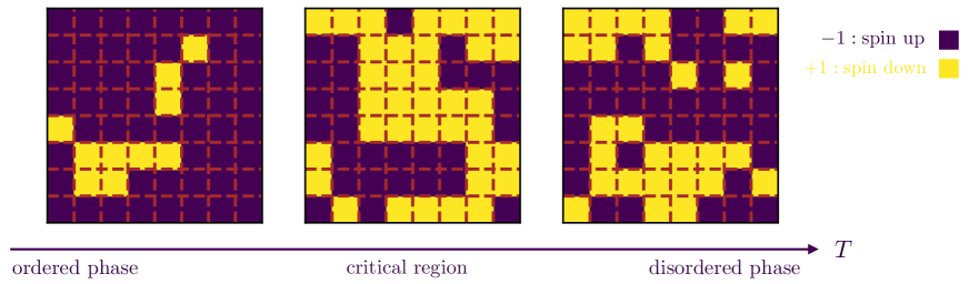
Figure 3: Ising configurations on an $8\times 8$ lattice sampled via mcmc simulations. Spins at neighbouring sites try to align along the same direction. The order parameter, the net magnetization, which is given as the sum of all $64$ spins is non-vanishing in the ordered phase below the critical temperature and (abruptly in infinite volume) vanishes when the system enters the disordered phase at higher temperatures.

To extract the relevant physics of the Ising system the vrbm should be exposed to spin configurations $s$ sampled at various temperatures below and above the critical region. As noticed in [24] (a behaviour also verified for our vrbm), even without training an rbm in the vicinity of $T_{c}$, but only below and above, the generative model is still able to capture the physics signalling a phase transition. Via Markov chain Monte Carlo (mcmc) simulations we thus produce a large number of spin configurations $s$ at various temperatures $T=0.1,0.2,..,4.5$ which we split into a training and test set of $60\,000$ and $10\,000$ samples, respectively. Our target distribution $q(\textbf{v})$ thus extends over the simulated Ising domain with $v^{(\alpha-1)\cdot L+\beta}=s^{\alpha\beta}$.

At this stage, revealing essentially the final outcome is in order. In [24, 22] the learning capacity of the ordinary rbm on the Ising model has been extensively studied showing that there exist three distinct learning phases depending on the relation between the number of hidden units $z_{0}$ and the total number of spins $N=L\times L$. For $z_{0}<N$ the rbm does not have enough resources to fully learn the target distribution from the Ising system. In this regime with less hidden than observable units, an appropriately trained generative model has still learned important features of the underlying Ising theory. In particular, the rbm flow seems to trigger a flow of spins very reminiscent of the Renormalization Group [25]. We plan to come back to this tantalizing finding in conjunction with varying number of hidden units and different training metrics in a later work. When $z_{0}=N$ the rbm fully learns to reproduce the Ising theory of nearest-neighbour interactions at any temperature. Finally, over-learning starts to occur for $z_{0}>N$ and the rbm increasingly learns irrelevant noice of thermodynamic fluctuations with increasing number of hidden units.

Specifics of the training.

For our purposes, we have trained various generative models at a chemical potential $\mu$ of slightly different designs which fall within the class described in Section 2.3. Since such designer choices do not influence the final outcome for sufficiently large number $K$ of available hidden units, we concentrate here, for concreteness and clarity of presentation, on the ansatz (2.9) with $p=1$. Our mean-field theoretic ansatz (2.24) to train our model by numerically solving the extremization problem posed in paragraph 2.2 converges to a satisfactory level already after $k=2$. Once exposed to various temperatures, any self-regularizing generative model should be able to track down the clearly defined regime of optimal training, $z=N$, detecting the physical interactions of nearest-neighbouring spins.

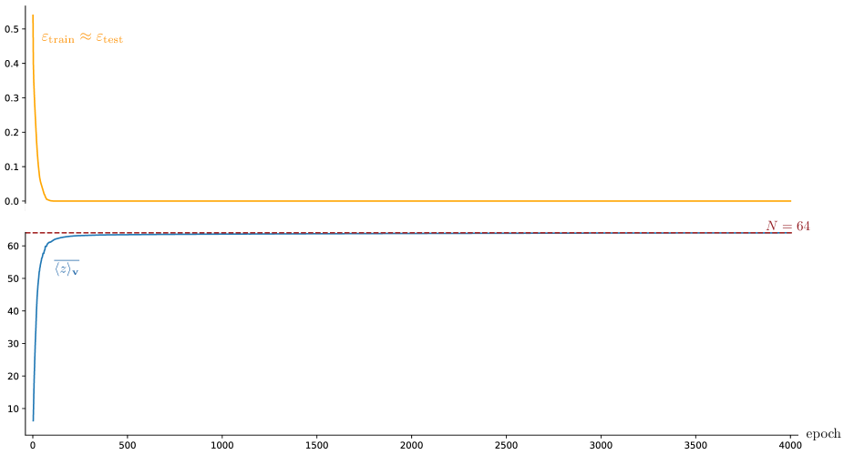
Figure 4: The train (3.32) and test (3.34) error as well as the average of the expectation value of the number of hidden units (3.37) are plotted while training the vrbm with $K=2\,000$ for $4\,000$ epochs.

Indeed, as seen in the upper Plot 4, our vrbm with $K=2\,000$ hidden units appropriately learns after a couple of epochs the two-dimensional Ising system. The exceedingly small training and test quadratic error, $\varepsilon_{\text{train}}=\varepsilon_{\text{test}}=\mathcal{O}\left(10^{-13}\right)$ as calculated without rounding by Eq. (3.32) and (3.34), respectively, effectively coincide throughout most of the training. To comprehend this order of magnitude, note that an ordinary rbm with (fixed) number of hidden units already of order $z_{0}=\mathcal{O}\left(100\right)$ leads for the same Ising configurations of total lattice size $N=64$ to a considerable test error $\varepsilon_{\text{test}}=\mathcal{O}\left(0.1\right)$. In fact, one does not even need to take $K$ that large to observe this self-regularizing character. A vrbm with $K=200$ only, effectively demonstrates the same learning curve as in Figure 4 once trained over the same data set. Sampling from those trained vrbm leads to perfect reconstructions of the original Ising data. The chemical potential Eq. (2.26) which is dynamically determined throughout training remains an order one quantity; specifically for the Ising model we get $\mu\approx 1.01$.

To understand what the vrbm has actually learned and how it did that, we plot in the lower part of Figure 4 the average of the expectation for the number of hidden units (see Eq. (2.20)) conditioned on the Isisng data,

$$\overline{\langle z\rangle_{\textbf{v}}}=\sum_{\textbf{v}}q(\textbf{v})\langle z\rangle_{\textbf{v}}~{},$$ (3.37)

over the course of learning epochs, together with the learning error. We clearly see that the model starts learning when $\langle z\rangle_{\textbf{v}}$ becomes $\mathcal{O}\left(N\right)$. Along similar lines, Figure 5 depicts the conditional probability $p(z|\textbf{v})$ defined in Eq. (2.12), averaged over the dataset,

$$\overline{p(z|\textbf{v})}=\sum_{\textbf{v}}q\left(\textbf{v}\right)p\left(z|\textbf{v}\right)$$ (3.38)

for different number of available resources, $K=128,400,2\,000$, ranging from $K=2N$ towards the formally desired regime $K\gg N$. On the one hand, it is clear that networks of hidden size between $z\approx 60$ and $z\approx 70$ receive a significant probability to participate into feature extraction. Thus, the vrbm still slightly over-learns due to finite – $K$ effects, with a test error $\varepsilon_{\text{test}}$ though, which is essentially zero for any practical purpose. On the other hand, we observe that the curve of $p(z|\textbf{v})$ becomes narrower around the critical value $z=64$ with increasing $K$. This is nothing but a manifestation of “the law of large numbers”: at the theoretical limit $K\rightarrow\infty$ we anticipate the vrbm to precisely pick $z=64$ as the most optimal size of the hidden layer to learn the provided Ising configurations.

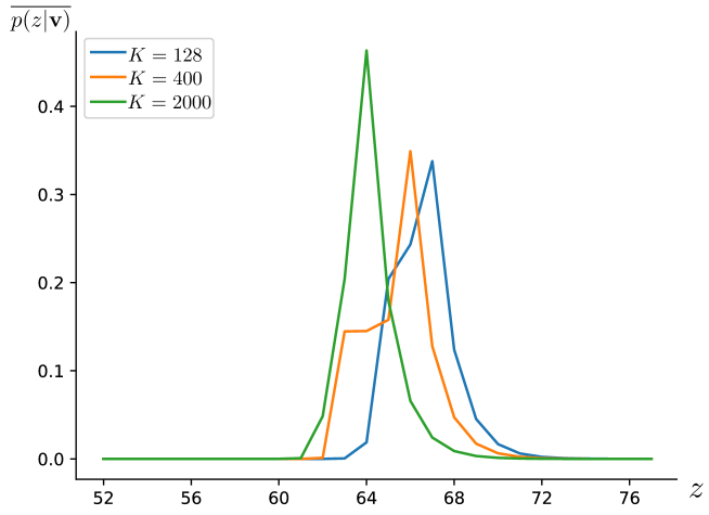
Figure 5: The average of the conditional probability Eq. (3.38) over the Ising data from the square lattice of length $L=8$ is plotted for different lengths $z$ of the hidden layer in the model with maximally $K=128,400,2\,000$ hidden units. The probability clearly exhibits a peak around $N=L^{2}=64$. For clarity, the plot concentrates on the region around $z=N$ given that networks of sizes away from it quickly get exponentially suppressed.

To further comprehend the behaviour of the grand-canonical generalization of rbm under training, we examine the value of the trained parameters from the perspective of the hidden units. The meaningful quantities to look at are the hidden biases $\beta_{a}$ and the average

$$\overline{\left|w_{a}\right|}=\mbox{$\frac{1}{N}$}\sum_{i=1}^{N}\left|w_{ai}\right|$$ (3.39)

entering the chemical potential via Eq. (2.28). For the first $a=1,...,400$ hidden units of the trained vrbm with $K=2\,000$ these are plotted in Figure 6. As theoretically anticipated, we recognize that the vrbm has effectively set to zero all weights $w_{ai}$ for $a>N$ in accordance with its self-regularizing character. In the language of paragraph 2.3 thus, $K_{\text{eff}}\approx N$. The latter $1\,600$ hidden units not depicted in Figure 6 follow an evident pattern for $a>K_{\text{eff}}$ and decouple from the feature detector (see schematic depiction in Figure 2). Incidentally, due to the aforementioned regularizing character also at smaller $K$, the depicted profile in Figure 6 looks effectively the same also when $K=400$ and even $K=128$. Most interestingly, the value of the first $K_{\text{eff}}$ hidden biases $\beta_{a}$ is smaller than the corresponding weight scale set by Eq. (3.39). Thus, these $\beta_{a}$ do not participate much in the modelling of Ising interactions performed by the first $K_{\text{eff}}\times N$ weights $w_{ai}$ (in the sense of Figure 7). The model then uses the remnant $(K-K_{\text{eff}})$ biases to adjust the value of the chemical potential $\mu\equiv\mu(w_{ai},\beta_{a})$ and its regularizing effect without crucially interfering with the actual feature detection.

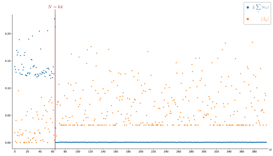
Figure 6: The scatter diagram depicts the row-average over the absolute value of weights $w_{ai}$ defined in Eq. (3.39) together with the absolute value of hidden biases $\beta_{a}$ for the first $a=1,...,400$ after training a vrbm with $K=2\,000$ for $4\,000$ epochs.

Another quantity of interest that is meaningful to examine for energy-based generative models is the free energy $F(\textbf{v})$ defined in Eq. (2.5). An estimation of its value is given by the grand-canonical expectation value of the free energy introduced in Eq. (2.3),

$$\langle F(\textbf{v},z)\rangle=\sum_{z=1}^{K}p\left(z|\textbf{v}\right)F(\textbf{v},z)~{},$$ (3.40)

under the conditional probability Eq. (2.12) of our model. For binary systems it is straight-forward [1] to expand $F(\textbf{v},z)$ in powers of $v^{i}$ and resum using that $(v^{i})^{2}=1$. In [23] the leading terms in the spin expansion were computed,

$$F(\textbf{v},z)=-\sum_{i=1}^{N}J^{z}_{i}v^{i}-\sum_{i,j}^{N}v^{i}\,S_{ij}^{z}\,v^{j}+...~{},$$ (3.41)

in terms of the spin current $J^{z}$ and the correlation matrix $S^{z}$ of a network with $z$ hidden units. For reasonably small values of the trained parameters $\lambda$ the two scale as

$$J^{z}_{i}=c_{i}+\sum_{a=1}^{z}b^{a}w_{ai}+\mathcal{O}\left(\lambda^{3}\right)\quad\text{and}\quad S_{ij}^{z}=\sum_{a=1}^{z}w_{ai}\,w_{aj}+\mathcal{O}\left(\lambda^{3}\right)\quad\text{for}\quad i\neq j$$ (3.42)

and $S_{ii}=0$, since $(v^{i})^{2}=1$ gives an irrelevant constant energy shift.

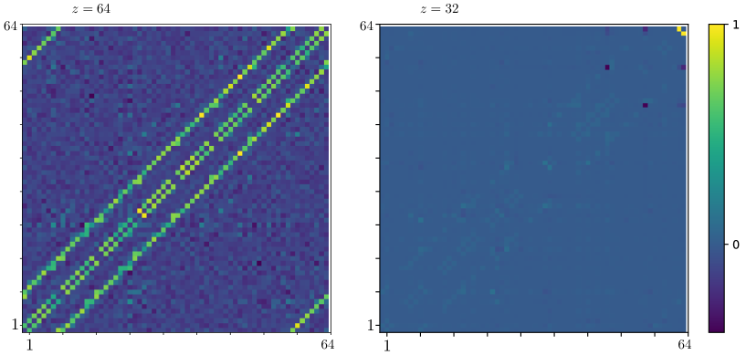
Figure 7: The heat map chart represents the interaction matrix $S^{z}$ defined in Eq. (3.42), normalized over its largest absolute value, for two networks with hidden sizes $z=32,64$ using the parameters of the vrbm with $K=2\,000$ trained over $4\,000$ epochs on the Ising data from the $64\times 64$ lattice.

Already in this crude approximation the current $J^{z}$ evaluated on the trained parameters $\lambda$ appears subleading to the spin-spin interaction term (cf. also Figure 6), as anticipated given that the Ising data was originally sampled at zero external magnetic field. In Figure 7, we draw the correlation matrix $S^{z}$ for different hidden-layer sizes $z$. (Note that the heat map chart of $S^{z}$ for $z>N$ will not look different from $z=64$, as $w_{ai}\approx 0$ for $a>N$.) After our preceding discussion, there is no surprise that networks with $z<N$ cannot satisfactory learn the input data. Their contribution to the approximation (3.40) to grand-canonical free energy is exponentially suppressed by $p(z|\textbf{v})$ as seen in Figure 5. In contrast, approaching $z=N$ the nearest-neighbour structure of the Ising data becomes apparent, at least to quadratic order in the spin expansion. The latter are precisely the networks which get significantly selected by Eq. (3.40) to participate in forming our estimation of the free energy of the vrbm model. In a future work, we plan to come back to the intriguing question of the order-by-order equivalence among the energies from the trained vrbm and the Ising model by formal resummation of the appropriate free energy Eq. (2.5) in the spirit of Eq. (3.41).

3.2 The dataset of handwritten digits

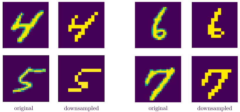
Figure 8: Examples from the mnist data set downsampled to $14\times 14$ pixel size and binarized.

As a first step in benchmarking ai models it is customary to draw samples from the nist database of “Handprinted Forms and Characters”. By now, a typical list of examples used throughout ml literature is the mnist data set [45] of handwritten digits from 0 to 9. It consists of $60\,000$ training and $10\,000$ test preprocessed images given in rgb format with an original $28\times 28$ pixel resolution. Let such a sample image be described by an integer matrix of rgb pixel intensities $S^{AB}\in[0,255]$ with $A,B=1,...,28$.

For our demonstrative purposes, it suffices to consider a reduced version of the mnist data by downsampling to a $14\times 14$ image version. This can be done via so called max or mean pooling [46, 47]. Concretely, each $2\times 2$ block of pixels in the original pixel matrix $S$ is replaced by either their average or their maximum leading for example to

$$\sigma^{\alpha\beta}:=\text{max}\{S^{2\alpha-1,2\beta-1},S^{2\alpha,2\beta-1},S^{2\alpha-1,2\beta},S^{2\alpha,2\beta}\}\quad\text{with}\quad\alpha,\beta=1,...,L~{},$$ (3.43)

and similarly for their average. In our case, $L=14$. To smoothen the resulting image $\sigma$ and to reduce its size while preserving important information for the feature detector it is possible to apply additional space-convolution filters (adding a padding frame where necessary) like

$$\tilde{\sigma}^{\alpha\beta}:=\mbox{$\frac{1}{4}$}\left(\sigma^{\alpha\beta}+\sigma^{\alpha,\beta+1}+\sigma^{\alpha+1,\beta}+\sigma^{\alpha+1,\beta+1}\right)~{},$$ (3.44)

which captures an average pixel intensity in overlapping $2\times 2$ blocks. Throughout the down-sampling and convolutional process we always make sure that the pixel center of mass, defined by

$$\begin{pmatrix}\alpha_{\text{cm}}\\ \beta_{\text{cm}}\end{pmatrix}=\left(\sum_{\alpha^{\prime},\beta^{\prime}=1}^{L}\sigma^{\alpha^{\prime}\beta^{\prime}}\right)^{-1}\sum_{\alpha,\beta=1}^{L}\sigma^{\alpha\beta}\begin{pmatrix}\alpha\\ \beta\end{pmatrix}~{},$$ (3.45)

coincides with the geometrical center of the image located at $\left(L/2,L/2\right)$ in order to filter out translational symmetry. Furthermore, to make contact with the preceding paragraph on the Ising model we turn to black and white images via binarizing all pixels simply by rounding each normalized pixel to its nearest integer (i.e. 0 or 1). Hence, our training input is given by $v^{(\alpha-1)\cdot L+\beta}=s^{\alpha\beta}$ with

$$s^{\alpha\beta}:=2\left\lfloor\frac{\sigma^{\alpha\beta}}{255}\right\rceil-1~{},$$ (3.46)

where we again arrange for $s^{\alpha\beta}\in\{-1,1\}$ consistent with the conventions introduced in Section 2.1. An example of the target images we are going to use in the following paragraph to train our vrbm is given in Figure 8.

Specifics of the training.

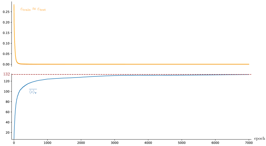
Figure 9: The train (3.32) and test (3.34) error as well as the average of the expectation value of the number of hidden units (3.37) are plotted while training the vrbm with $K=900$ for $7\,000$ epochs.

Similar to the Ising model, we train vrbm of different designs ($p=1,2$ in the chemical potential Eq. (2.26)) on the downsampled mnist data of observable size $N=L^{2}=196$ and recover the law of large numbers. With increasing number of available hidden resources the outcome stabilizes and effectively becomes independent of $K$. The train and test loss errors, Eq. (3.32) and (3.34), quickly become $\mathcal{O}\left(10^{-8}\right)$ and $\mathcal{O}\left(10^{-5}\right)$, respectively, signalling a very good convergence and a small over-learning. As a reference, an ordinary rbm with $z=200$ trained on the exact same data without any form of regularization has a test error of $\mathcal{O}\left(10^{-3}\right)$. In Figure 9, the loss errors are plotted over the learning epochs as well as the average of the expectation value for the size of hidden layer Eq. (3.37). Again, our ml model starts learning when networks of a given size around $\overline{\langle z\rangle_{\textbf{v}}}\approx 132$ become more and more favourable. The chemical potential is dynamically determined during training to $\mu\approx 1.1$.

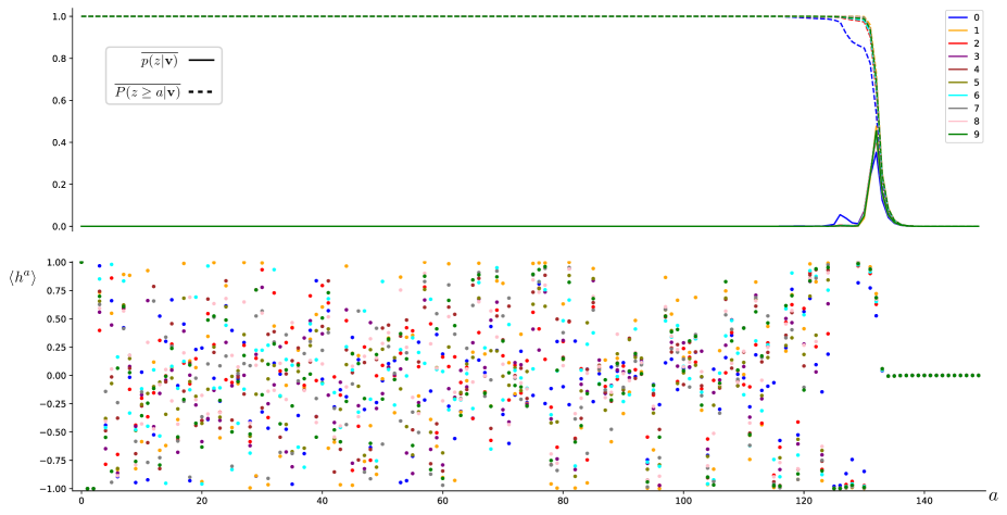
Figure 10: Continuous lines in the upper plot depict the average of conditional probability Eq. (2.12) over the mnist data for each handwritten digit 0,…,9 (the color pattern applies also to the scatter plot) of a trained vrbm with $K=900$ hidden units. Networks with bigger $z$ are exponentially suppressed and are not presented in the graph for clarity, $z,a=1,...,150$. Dashed lines depict the corresponding ccdf in Eq. (2.19). The lower scatter diagram presents the expectation value of hidden units as deduced from Eq. (2.18) digit-wise conditioned on the input data.

To obtain a better feeling of what the vrbm has learned from the dataset of handwritten digits it is sensible to look at the average of conditional probability Eq (3.38) over each digit from mnist, separately. From the upper part of Figure 10 it becomes clear that for all digits the most probable size of the hidden layer coincides with the (rounded) average $\left\lfloor\overline{\langle z\rangle_{\textbf{v}}}\right\rceil=132$. Still, for an “easy” digit like zero there appears a lower pump already before $z$ approaches the region of $\overline{\langle z\rangle_{\textbf{v}}}$. Such a profile for ${p(z|\textbf{v})}$ is typical for a system coming from everyday life and is comparatively richer to the Ising paradigm of the previous section, where all data came from the same microscopic Hamiltonian Eq. (3.36).

To avoid any confusion, the scatter diagram in the lower part of Figure 10 emphasizes that the probability $p(z|\textbf{v})$ according to which the size of the hidden layer gets selected is a different concept from the actual feature detection happening at the level of $\langle h^{a}\rangle_{\textbf{v}}$. Depending on the digit they track, hidden units $h^{a}$ are more or less likely to get activated with a given sign. Of course, the two concepts are intimately connected via Eq. (2.18): the complementary cumulative distribution associated to $z$ modulates the profile of $\langle h^{a}\rangle_{\textbf{v}}$. The hidden units $h^{b}$ with $b>K_{\text{eff}}$ of larger hidden networks, whose probability to be selected becomes exponentially suppressed, remain deactivated. Stochastically, the equivalent statement would be that those $h^{b}$ receive an equal probability to be $\pm 1$, behaving like free units, as they have decoupled from connected Boltzmann machine in Figure 2.

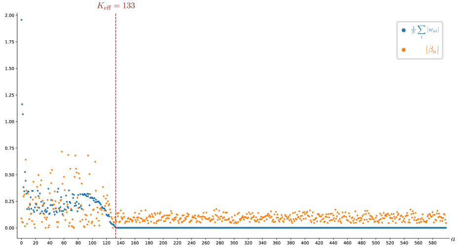
Figure 11: The scatter diagram depicts the row-average over the absolute value of weights $w_{ai}$ defined in Eq. (3.39) together with the absolute value of hidden biases $\beta_{a}$ after training a vrbm with $K=900$ for $7\,000$ epochs.

Indeed, the weights for $a>K_{\text{eff}}=133$ have been effectively regularized to zero, as deduced from Figure 11. Hence, the corresponding hidden units to the far right of the plot decouple in the sense of the schematic depiction in Figure 2. The scatter plot 11 follows the same regularizing concept as the Ising plot 6 and we refer the reader to the corresponding paragraph in Section 3.1 about the Ising model. An obvious difference observed in the two plots for the first $a=1,...,K_{\text{eff}}$ hidden units lies in the different character of the systems: Concerning the mnist dataset, hidden biases $\beta_{a}$ actively participate in feature detection in contrast to the Ising scenario in absence of external magnetic fields.

4 Conclusions and outlook

In this paper, we have considered (shallow) restricted Boltzmann machines at a finite chemical potential $\mu$. In principle, such a grand-canonical extension of the rbm performs feature extraction from a target distribution $q(\textbf{v})$ by invoking hidden layers $\{h^{a}\}_{a=1,...,z}$ of various length $z=1,...,K$ to model interactions among $N$ observables units $v^{i}$, where in principle $K\gg N$. We have concentrated on an intuitive choice of the chemical potential as a function of a “vacuum” energy, which essentially measures the added norms of the weight matrix $\omega_{ai}$ and bias vector $\beta_{a}$ per unit $h^{a}$ actively participating in feature extraction. The appropriately trained vrbm at such chemical potential $\mu\equiv\mu(\left|\omega_{ai}\right|,\left|\beta_{a}\right|)$ is able to track down (up to $N/K$–suppressed effects) the optimal length of the hidden layer to model provided data points. To do so, the vrbm mainly uses the biases $\beta_{c}$ of disconnected ($\omega_{ci}=0$) hidden units $h^{c}$ to regulate the number of hidden units $K_{\text{eff}}$ which actively participate in feature extraction, manifesting the self-regularizing character of the model.

Incorporating this regularizing character in the form of a chemical potential has many advantages, besides the formal simplicity of Legendre-transforming to the grand-canonical ensemble, which allows us to keep most of the techniques implemented to train ordinary Boltzmann machines intact. By maximizing the expectation value of $\log$-probability of the modelled data under $q(\textbf{v})$ the value of $\mu$ is dynamically fixed during training, already from the very first epochs. Thus, the probability to use unnecessary long hidden layers is quickly regularized to zero so that the cd algorithm only needs to update at most the parameters corresponding to the relevant $K_{\text{eff}}\ll K$ hidden units. As the probability to use a hidden layer of a certain length $z$ is conditioned on the obserbable data v, the grand-canonical theory makes sure to always assign enough hidden resources to model a given subset of the target distribution $q(\textbf{v})$ while avoiding overfitting. This feaure of the vrbm is to be contrasted with the standard $\ell_{p}$ – regularization globally implemented in the canonical Boltzmann machine at the level of the full data set.

The merits of training the suggested grand-canonical extension to the rbm have been rigorously verified on the Ising and mnist data sets. In both cases, the vrbm efficiently converges towards optimal choices for the sizes of the hidden layer leading to a very good generalization error on previously unseen data. In order to get a feeling of how the vrbm regulated itself and learned the desired features we have plotted various quantities during and after training. In particular, we observe that the grand-canonical theory with dynamically determined chemical potential presents an extremely similar behaviour to its canonical cousin as a feature detector, once the regularization of $(K-K_{\text{eff}})$ hidden units has taken place in the first steps of training. In contrast to the trial-and-error approach mostly implemented throughout the literature to pick some optimal size for the hidden layer of the rbm to extract the traits from a given data set, the vrbm managed to efficiently come to the same conclusion by dynamically regulating itself during training.

Future directions.

In this work, we have focused on a concrete ansatz Eq. (2.30) concerning the form of the chemical potential dictated by symmetries, intuition and some rather general assumptions on the form of the input data. At the formal level, investigating the various phases of the grand-canonical Boltzmann system in conjunction with the extremization of the target function in the spirit of [48] remains an open question. In a more applied fashion, one could relax some of our working assumptions in Section 2.3 or try to specifically address different target data by building biases into the form of $\mu$. Considering more versatile data sets would not only deliver stronger evidence on the self-regularizing character, but also help exhibit the flexibility of vrbm at implementing a hidden layer of different sizes depending on the specifics of the concrete data point being modelled.

To clearly outline the novel aspects when training in the grand-canonical ensemble with a penalizing chemical potential, our test setting has been rather minimalistic. As a subsequent step, one could combine the theory at finite chemical potential with other techniques of regularization (like $\ell_{p}$ – norm) already implemented in the literature. Another aspect for future study is to extend the domain v of the vrbm to address multimodal distributions and data represented on the real numbers. Last but not least, deeper networks like deep belief networks (dbn) and deep Boltzmann machines (dbm) are the next natural candidates to apply similar regularization techniques both at the level of the depth of the full network as well as the length of each hidden layer.

Acknowledgments

The author would like to thank Rudolf Mayer and Deb Sarkar for very useful discussions on the topic as well as Stefan Groot Nibbelink for proof reading the manuscript. This work is supported within the SBA-K1 program. The competence center SBA Research (SBA-K1) is funded within the framework of comet – Competence Centers for Excellent Technologies by bmvit, bmdw, and the federal state of Vienna, managed by the ffg.

References

- [1] P. Mehta, M. Bukov, C.-H. Wang, A. r. G. R. Day, C. Richardson, C. K. Fisher, and D. J. Schwab, A high-bias, low-variance introduction to Machine Learning for physicists, arXiv e-prints (2018), arXiv:1803.08823, arXiv:1803.08823 [physics.comp-ph].
- [2] G. Carleo and M. Troyer, Solving the quantum many-body problem with artificial neural networks, Science 355 (2017), no. 6325, 602, https://science.sciencemag.org/content/355/6325/602.full.pdf.
- [3] T. Vieijra, C. Casert, J. Nys, W. De Neve, J. Haegeman, J. Ryckebusch, and F. Verstraete, Restricted Boltzmann Machines for Quantum States with Nonabelian or Anyonic Symmetries, arXiv e-prints (2019), arXiv:1905.06034, arXiv:1905.06034 [cond-mat.str-el].
- [4] Y. Levine, D. Yakira, N. Cohen, and A. Shashua, Deep Learning and Quantum Entanglement: Fundamental Connections with Implications to Network Design, arXiv e-prints (2017), arXiv:1704.01552, arXiv:1704.01552 [cs.LG].
- [5] D.-L. Deng, X. Li, and S. Das Sarma, Quantum entanglement in neural network states, Phys. Rev. X 7 (2017), 021021.
- [6] P. T. Komiske, E. M. Metodiev, and M. D. Schwartz, Deep learning in color: towards automated quark/gluon jet discrimination, Journal of High Energy Physics 2017 (2017), no. 1, 110.
- [7] B. P. Roe, H.-J. Yang, J. Zhu, Y. Liu, I. Stancu, and G. McGregor, Boosted decision trees as an alternative to artificial neural networks for particle identification, Nuclear Instruments and Methods in Physics Research Section A: Accelerators, Spectrometers, Detectors and Associated Equipment 543 (2005), no. 2-3, 577.
- [8] P. Baldi, P. Sadowski, and D. Whiteson, Searching for exotic particles in high-energy physics with deep learning, Nature communications 5 (2014), 4308.
- [9] F. Ruehle, Evolving neural networks with genetic algorithms to study the string landscape, Journal of High Energy Physics 2017 (2017), no. 8, 38.
- [10] Y.-H. He, Deep-learning the landscape, arXiv preprint arXiv:1706.02714 (2017).
- [11] Y.-H. He, The calabi-yau landscape: from geometry, to physics, to machine-learning, arXiv preprint arXiv:1812.02893 (2018).
- [12] K. Hashimoto, S. Sugishita, A. Tanaka, and A. Tomiya, Deep learning and the ads/cft correspondence, Physical Review D 98 (2018), no. 4, 046019.
- [13] W.-C. Gan and F.-W. Shu, Holography as deep learning, International Journal of Modern Physics D 26 (2017), no. 12, 1743020.
- [14] Y.-Z. You, Z. Yang, and X.-L. Qi, Machine learning spatial geometry from entanglement features, Physical Review B 97 (2018), no. 4, 045153.
- [15] M. Guillaumin, J. Verbeek, and C. Schmid, Multimodal semi-supervised learning for image classification, 06 2010, pp. 902–909.
- [16] X. Dong and L. Zhou, Geometrization of deep networks for the interpretability of deep learning systems, arXiv e-prints (2019), arXiv:1901.02354, arXiv:1901.02354 [cs.LG].
- [17] S. N. Shah, Variational approach to unsupervised learning, 04 2019.
- [18] P. Mehta and D. J. Schwab, An exact mapping between the Variational Renormalization Group and Deep Learning, arXiv e-prints (2014), arXiv:1410.3831, arXiv:1410.3831 [stat.ML].
- [19] G. Torlai and R. G. Melko, Learning thermodynamics with Boltzmann machines, prb 94 (2016), no. 16, 165134, arXiv:1606.02718 [cond-mat.stat-mech].
- [20] S. Goldt and U. Seifert, Thermodynamic efficiency of learning a rule in neural networks, New Journal of Physics 19 (2017), no. 11, 113001, arXiv:1706.09713 [cond-mat.stat-mech].
- [21] J. Tubiana and R. Monasson, Emergence of Compositional Representations in Restricted Boltzmann Machines, Phys. Rev. Lett. 118 (2017), no. 13, 138301, arXiv:1611.06759 [physics.data-an].
- [22] A. Morningstar and R. G. Melko, Deep Learning the Ising Model Near Criticality, arXiv e-prints (2017), arXiv:1708.04622, arXiv:1708.04622 [cond-mat.dis-nn].
- [23] G. Cossu, L. Del Debbio, T. Giani, A. Khamseh, and M. Wilson, Machine learning determination of dynamical parameters: The Ising model case, arXiv:1810.11503 [physics.comp-ph].
- [24] S. Iso, S. Shiba, and S. Yokoo, Scale-invariant Feature Extraction of Neural Network and Renormalization Group Flow, Phys. Rev. E97 (2018), no. 5, 053304, arXiv:1801.07172 [hep-th].
- [25] S. S. Funai and D. Giataganas, Thermodynamics and Feature Extraction by Machine Learning, arXiv:1810.08179 [cond-mat.stat-mech].
- [26] P. M. Lenggenhager, Z. Ringel, S. D. Huber, and M. Koch-Janusz, Optimal Renormalization Group Transformation from Information Theory, arXiv e-prints (2018), arXiv:1809.09632, arXiv:1809.09632 [cond-mat.stat-mech].
- [27] M. Koch-Janusz and Z. Ringel, Mutual information, neural networks and the renormalization group, Nature Physics 14 (2018), no. 6, 578, arXiv:1704.06279 [cond-mat.dis-nn].
- [28] E. T. Jaynes, Information Theory and Statistical Mechanics, Physical Review 106 (1957), no. 4, 620.
- [29] A. Rényi et al., On measures of entropy and information, in Proceedings of the Fourth Berkeley Symposium on Mathematical Statistics and Probability, Volume 1: Contributions to the Theory of Statistics, The Regents of the University of California, 1961.
- [30] R. Pascanu, T. Mikolov, and Y. Bengio, On the difficulty of training recurrent neural networks, in International conference on machine learning, 2013, pp. 1310–1318.
- [31] S. Ioffe and C. Szegedy, Batch normalization: Accelerating deep network training by reducing internal covariate shift, CoRR abs/1502.03167 (2015), 1502.03167.
- [32] G. E. Hinton, A practical guide to training restricted boltzmann machines, Neural networks: Tricks of the trade, Springer, 2012, pp. 599–619.
- [33] T. Domhan, J. T. Springenberg, and F. Hutter, Speeding up automatic hyperparameter optimization of deep neural networks by extrapolation of learning curves, in Twenty-Fourth International Joint Conference on Artificial Intelligence, 2015.
- [34] F. Girosi, M. Jones, and T. Poggio, Regularization theory and neural networks architectures, Neural Computation 7 (1995), no. 2, 219, https://doi.org/10.1162/neco.1995.7.2.219.
- [35] I. Goodfellow, Y. Bengio, and A. Courville, Deep learning, MIT Press, 2016, http://www.deeplearningbook.org.
- [36] G. E. Hinton, T. J. Sejnowski, et al., Learning and relearning in boltzmann machines, Parallel distributed processing: Explorations in the microstructure of cognition 1 (1986), no. 282-317, 2.
- [37] M.-A. Côté and H. Larochelle, An Infinite Restricted Boltzmann Machine, arXiv e-prints (2015), arXiv:1502.02476, arXiv:1502.02476 [cs.LG].
- [38] E. Nalisnick and S. Ravi, Infinite dimensional word embeddings.
- [39] X. Peng, X. Gao, and X. Li, On better training the infinite restricted boltzmann machines, Machine Learning 107 (2018), no. 6, 943.
- [40] C. M. Bishop, Pattern recognition and machine learning, springer, 2006.
- [41] B. Wang and D. Klabjan, Regularization for unsupervised deep neural nets, in Thirty-First AAAI Conference on Artificial Intelligence, 2017.
- [42] D. J. C. MacKay, Information theory, inference, and learning algorithms, Copyright Cambridge University Press, 2003.
- [43] L. Onsager, Crystal statistics. i. a two-dimensional model with an order-disorder transition, Physical Review 65 (1944), no. 3-4, 117.
- [44] R. J. Baxter, Exactly solved models in statistical mechanics, Elsevier, 2016.
- [45] Y. Lecun, L. Bottou, Y. Bengio, and P. Haffner, Gradient-based learning applied to document recognition, Proceedings of the IEEE 86 (1998), no. 11, 2278.
- [46] J. Masci, U. Meier, D. Cireşan, and J. Schmidhuber, Stacked convolutional auto-encoders for hierarchical feature extraction, in International Conference on Artificial Neural Networks, Springer, 2011, pp. 52–59.
- [47] K. Sohn and H. Lee, Learning invariant representations with local transformations, arXiv preprint arXiv:1206.6418 (2012).
- [48] A. Decelle, G. Fissore, and C. Furtlehner, Thermodynamics of Restricted Boltzmann Machines and Related Learning Dynamics, Journal of Statistical Physics 172 (2018), no. 6, 1576, arXiv:1803.01960 [cond-mat.dis-nn].