A Deep Convolutional Network for Seismic Shot-Gather Image Quality Classification

Abstract

Deep Learning-based models such as Convolutional Neural Networks, have led to significant advancements in several areas of computing applications. Seismogram quality assurance is a relevant Geophysics task, since in the early stages of seismic processing, we are required to identify and fix noisy sail lines. In this work, we introduce a real-world seismogram quality classification dataset based on 6,613 examples, manually labeled by human experts as good, bad or ugly, according to their noise intensity. This dataset is used to train a CNN classifier for seismic shot-gathers quality prediction. In our empirical evaluation, we observe an F1-score of 93.56% in the test set.

Keywords Deep Learning  $\cdot$ CNN  $\cdot$ Shot-Gather  $\cdot$ Quality classifier

1 Introduction

A classic challenge in the field of geophysics involves accurately estimating the characteristics of the Earth’s subsurface based on measurements acquired by sensors on the surface. Seismic reflection is one of the most widely used methods. It involves generating seismic waves using controlled active sources on the surface (e.g., dynamite explosions in land acquisition or air guns in marine acquisition), and further collecting the reflected data with sensors located above the area [1]. The term shot refers to a firing by one of these sources. By grouping the seismic signals resulting from the same shot and registered by the sensors into a common-shot domain called the shot gather makes it possible to produce an image that represents information about that Earth’s subsurface area [2].

Seismic shot-gather quality classification is relevant for the early stages of seismic processing and noise removal. However, controlling seismic quality is challenging as it is traditionally very subjective and time-consuming and relies upon the valuable time from skilled and experienced experts. Thus, the application of machine learning for this problem is useful as it reduces the turnaround time by quickly identifying the bad quality shot lines, instead of visual and cumbersome quality control techniques.

Some previous work investigate applications of neural networks for geophysical signal classification. Valentine and Woodhouse [3], for instance, perform an automatic selection of high-quality seismic data to improve results from tomographic inversion. To accomplish that, they train an Artificial Neural Network (ANN) to recognize the frequency-domain characteristics of high and low-quality waveform. We share the same goal of selecting seismic data aimed by quality, but instead of classifying the waveforms individually, we take advantage of the typical shot-gather structure and build a classifier that makes an overall decision based on the correlated information presented between multiple traces. Jain et al. [4] utilize a Convolutional Neural Network (CNN) to perform a similarity-based classification [4, 5]. They define an objective similarity function based on the Triplet Network [6], which is a deep learning technique with widespread use in computer vision for the face recognition task. In order to apply this procedure, the authors build a Temporal Convolutional Network (TCN) and measure pairwise similarities between the seismograms using the Triplet loss function. Further, they evaluate their approach using the Receiver Operating Characteristic Curve and report 87% as the area under the curve (AUC) in K22A, which is the most active station in the test set from the database of USArray.

The main contributions of our work are twofold: (1) Describing the construction of a dataset for shot-gather image quality classification; (2) Presenting a comparative study of three deep learning-based approaches. The first one, using state-of-the-art CNNs for feature extraction combined that are fed to a SVM [7] classifier. The second one, introducing our CNN architecture for shot-gather image quality classification. And the last one, fine-tuning the previous CNN. Our proposed CNN architecture achieves the best results with 94.91%of F1-Score in a 10-fold cross-validation experiment.

The outline of this paper is structured as follows. Section 2 presents our dataset construction. Section 3 describe our proposed network. The experimentation and result analysis are presented in Section 4. And finally, Section 5 brings our final considerations.

2 Seismic shot-gather quality dataset

Our dataset consists of an offshore towed streamer data in a targeted region consisting $7,993$ shot-gathers with 8 cables each, thus containing a total of $63,994$ shot-gather images.

In a common shot-gather, the abscissa stands for the position of the sensor relatively to the shot position, whit this displacement being known as the offset distance. The ordinate represents the registered time of the signal, the larger this time, the deeper the signal reached the underground surface.

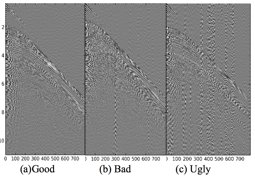
Figure 1: Examples of shot-gather images classified by a geophysicist as good, bad and ugly.

Out of the total generated images, $6,613$ were chosen and manually classified by a geophysicist, using good, bad and ugly labels, according to a visual inspection of artifacts related to swell noise and anomalous recorded amplitude. This process takes roughly ten hours of human labor. Figure 1 shows one example per class of shot-gather images classified by a geophysicist. From this figure, we observe that the good label represents clean images, while the ugly label represents images that have an intense presence of noise. The bad label represents those images who are neither fully clean, nor as noisy as the ugly class.

The table 1 shows the shot-gather quantity and proportion of the three labels. The dataset is more represented by good (66.68%), followed by the bad (31.54%) and the ugly (1.76%). This indicates that we are working with an acquisition, where good and bad labels almost dominate the entire representation. This dataset class imbalance is very challenging to machine learning algorithms, since they are data-intensive and we have just a few ugly shot-gather images. The Train represents 79% and Test 21%.

Table 1: Shot-gather images distribution over the three categories

	Good	Bad	Ugly	Total	(%)
Train	3,364	1,746	114	5,224	79.0
Test	1,064	340	3	1,389	21.0
Total	4,410	2,086	117	6,613	100
(%)	66.68	31.54	1.76	100

3 Minception Network

A typical CNN usually has a stack of convolutional layers with 3x3 or 5x5 kernels followed by a pooling layer. Due to the variance of shot-gather noise shape and scale, select an appropriate kernel size is a key challenge. The shot-gather image presented in Figure 2 shows examples of noise variations acquired through a seismic marine survey [8]. To detect larger noises, higher kernel sizes are more adequate, while to thin noises, small kernel sizes work better.

Inspired on GoogleNet’s Inception block [9], we suggest the use of both 3x3 and 5x5 kernel sizes at the same layer. In this way, during networking training, the internal layers automatically choose the kernel sizes that will be relevant to learn the required information.

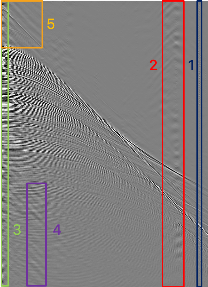
Figure 2: Example of noise variations in seismic marine survey made by Elboth et al. [8]: (1) Pressure Variation Noise; (2) Swell Noise; (3) Tugging/Strumming Noise; (4) Seismic Interference and (5) Proppeller Cavitation Noise.

The Figure 3 (A) shows the standard Minception block, a simplified version of Inception block with fewer parameters. Instead of using a single convolutional layer, we combine a 3x3 and 5x5 convolutions by concatenating their output in a single tensor forming the input of a 3x3 convolution that creates new filters by correlating the previous one.

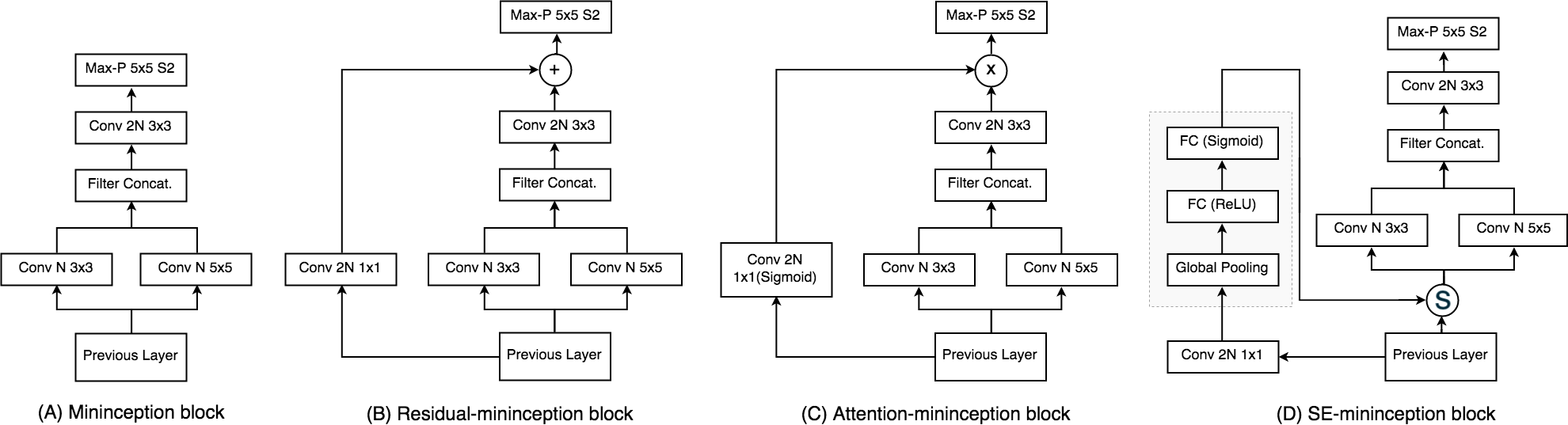
Figure 3: (A) Standard minception block. (B) Minception block with residual connection. (C) Minception block with self attention mechanism. (D) Minception combined with Squeeze-and-Excitation (SE) block.

Table 2 shows the Minception network structure, that is built on four stacked Minception blocks. All convolutional layers use ReLU nonlinearity, same padding, and stride 1. The $N$ hyperparameter indicates the number of kernels per layer, respectively equals to 1, 2, 4 and 8. A final downsampling is handled with a 5x5 max pooling with stride 2 to perform spatial dimensionality reduction. The last two layers, which are fully connected, has 32 units and feeds a softmax layer with 3 classes.

Table 2: MinceptionNet architecture

Component	output shape
Input image	299x299x1
Down-Sampling (Area interpolation)	99x99x1
Minception block 1 (N=1)	97x97x2
Max Pooling	47x47x2
Minception block 2 (N=2)	45x45x4
Max Pooling	21x21x4
Minception block 3 (N=4)	19x19x8
Max Pooling	8x8x8
Minception block 4 (N=8)	6x6x16
Max Pooling	1x1x16
Fully connected (ReLU)	32
Fully connected (Linear)	32
Softmax	3

We explored the other three variants of minception blocks using mechanisms of benchmarks networks for image classification. The first one, called (B) Residual-Minception uses the mechanism proposed by ResNet Network that has a goal to address the vanishing gradient problem of Deep Neural Networks. As described in [10] it’s empirically known that when we increase the depth of the network, the gradient gets saturated and then degrades rapidly. To solve it we want to experiment with the addition of a skip-connection to Standard Minception. However, to sum it properly, we need to previously add a convolution block 2N 1x1 in the skip-connection just to match with the shape from the output of Conv 2N 3x3.

The second variant, (C) Attention-Minception uses the mechanism of self-attention [11]. This mechanism is similar to the previous block as it has a skip-connection with a Convolutional Block, but in this particular case we use the sigmoid activation function instead of the standard ReLU, then it performed an element-wise multiplication.

The last Minception variant, (D) SE-Minception incorporates the channel attention mechanism provided by Squeeze and Excitation Module (SE) from SE-Net [12]. Squeeze and Excitation is a technique that improves the quality of representations produced by the network by learning global information from channels and dynamically emphasizing informative features. The process of SE is divided into three operations: (1) squeeze spatial information into a channel descriptor, (2) capture channel-wise dependencies targeting on important features and (3) perform a scale operation (channel-wise multiplication) in the original channels. The first operation is performed by a Global Average Pooling, which generates a summary of channel-wise statistics. The second operation is performed by two fully-connected (FC) layers in a row, where the first layer compress channel dimensionality by a given reduction ratio and the second layer increase channel dimensions back to the input channel size.

4 Experimental Evaluation

In this section, we evaluate the effectiveness of proposed approaches for seismic shot-gather image quality classification. First, we report the performance of the SVM classifier combined with transfer learning method. Next, we investigate the performance of our end-to-end CNN called MinceptionNet. And finally, we optimize the MinceptionNet exploring the trade-offs by tunning the network parameters based on two hyper-parameters, a width multiplier and a resolution multiplier.

4.1 Setup

We use Adam as the default optimizer and set the learning rate to 0.001, the batch size to 64, the training phase to 100 epochs with patience at 10 epochs, looking always for the best accuracy in the validation set.

The Dataset has imbalanced classes, whit the ugly label barely hitting 2% of the total. We perform a 10-fold cross-validation and evaluate the model by the F1-Score per class and the F1-weighted (F1-W), which is the sum of the F1-score for each class weighted by its proportion.

$$P_{l}=\frac{TP_{l}}{TP_{l}+FP_{l}}$$ (1)

$$R_{l}=\frac{TP_{l}}{TP_{l}+FN_{l}}$$ (2)

$$F1_{l}=\frac{2\times P(l)\times R_{l}}{P_{l}+R_{l}}$$ (3)

$$F1_{weigthed}=\sum_{l}^{|L|}{F1_{l}\times p_{l}}$$ (4)

Where $TP_{l},TN_{l},FP_{l}$, $FN_{l}$ and $p_{l}$ denote the examples that are true positives, true negatives, false positives, false negatives, and proportion of label $l$, respectively. The F1 score, defined in Equation 3, measures how precise the classifier by the harmonic mean between Precision (Equation 1) and Recall (Equation 2).

4.2 Baseline

For the baseline method, we use the SVM [7] classifier with input features provided by transfer learning. We use the output of a chosen hidden layer of a pre-trained CNN for the object recognition task. We use the inner layers of the VGG16, VGG19 [13] and InceptionV3 [14] with the network weights trained in the ImageNet classification dataset [15]. The workflow of this approach using the InceptionV3 network is illustrated in Figure 4.

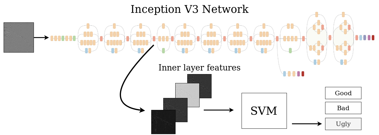
Figure 4: Workflow of our baseline. Given a shot-gather image, features extracted from intermediate convolutional layers. Then SVM is trained to predict the classification output.

CNNs when trained tend to learn at the first layers features that resemble either Gabor filters or color blobs. At the intermediate and final layers, the combination of these filters helps to extract relevant features from images, resulting in complex patterns [16]. Once we have extracted features from each layer, we then compare the performances of SVM classifier using each of them.

Tables 3, 4 and 5 summarize the results for VGG16, VGG19, and InceptionV3, respectively. The best model uses features extracted from VGG19’s block 2, which produces an F1-W of 90.82%. Next, VGG16’s block 2 is the second best model, achieving an F1-W of 88.99%. We can see that the Block 2 is the best for both networks, where we also get the best F1-Good and F1-Bad. Analysing VGG16 and VGG19 results, we observe that both models have similar results, but VGG19 is slightly better. InceptionV3 is our worst performing model, since it does not reach higher results than VGG19 or VGG16.

Table 3: F1-W and F1-score for Good (G), Bad (B) and Ugly (U) labels with SVM over the VGG16’s blocks

Block	F1-W (%)	F1-G (%)	F1-B (%)	F1-U (%)
0	83.03	91.8	66.58	45.95
	$\pm$ 0.45	$\pm$ 0.09	$\pm$ 0.29	$\pm$ 0.93
1	88.37	94.20	78.21	50.02
	$\pm$ 0.24	$\pm$ 0.16	$\pm$ 0.42	$\pm$ 1.34
2	88.99	95.08	81.48	49.96
	$\pm$ 0.30	$\pm$ 0.13	$\pm$ 0.35	$\pm$ 0.99
3	74.93	87.99	48.71	50.61
	$\pm$ 0.46	$\pm$ 0.05	$\pm$ 0.38	$\pm$ 1.36
4	36.51	47.98	14.39	0.36
	$\pm$ 6.62	$\pm$ 12.39	$\pm$ 6.95	$\pm$ 0.34

Table 4: F1-W and F1-score for good (G), bad (B) and ugly (U) labels with SVM over the VGG19’s blocks

Block	F1-W (%)	F1-G (%)	F1-B (%)	F1-U (%)
0	83.06	91.86	66.58	45.46
	$\pm$ 0.46	$\pm$ 0.08	$\pm$ 0.28	$\pm$ 0.86
1	87.76	93.94	76.87	48.78
	$\pm$ 0.38	$\pm$ 0.21	$\pm$ 0.67	$\pm$ 1.01
2	90.82	95.64	83.10	47.21
	$\pm$ 0.29	$\pm$ 0.18	$\pm$ 0.44	$\pm$ 1.53
3	81.49	90.8	63.59	50.14
	$\pm$ 0.58	$\pm$ 0.13	$\pm$ 0.64	$\pm$ 0.88
4	36.51	47.98	14.39	0.36
	$\pm$ 6.62	$\pm$ 12.39	$\pm$ 6.95	$\pm$ 0.34

Table 5: F1-W and F1-score for good (G), bad (B) and ugly (U) labels with SVM over the InceptionV3’s blocks

Block	F1-W (%)	F1-G (%)	F1-B (%)	F1-U (%)
0	86.02	93.23	73.07	45.56
	$\pm$ 0.30	$\pm$ 0.17	$\pm$ 0.55	$\pm$ 1.45
1	85.54	92.99	72.05	45.40
	$\pm$ 0.40	$\pm$ 0.17	$\pm$ 0.60	$\pm$ 1.10
2	81.01	90.89	62.13	45.22
	$\pm$ 0.52	$\pm$ 0.08	$\pm$ 0.53	$\pm$ 1.3
3	83.21	91.98	66.86	44.35
	$\pm$ 0.38	$\pm$ 0.14	$\pm$ 0.56	$\pm$ 1.14
4	81.5	91.23	63.04	43.77
	$\pm$ 0.45	$\pm$ 0.14	$\pm$ 0.59	$\pm$ 1.05
5	81.09	90.98	62.25	44.36
	$\pm$ 0.39	$\pm$ 0.11	$\pm$ 0.58	$\pm$ 1.52
6	77.92	89.63	55.07	44.19
	$\pm$ 0.51	$\pm$ 0.04	$\pm$ 0.47	$\pm$ 1.51
7	76.78	89.16	52.41	44.59
	$\pm$ 0.49	$\pm$ 0.0	$\pm$ 0.40	$\pm$ 1.50
8	83.05	91.99	66.36	43.58
	$\pm$ 0.41	$\pm$ 0.11	$\pm$ 0.48	$\pm$ 1.19
9	76.10	89.06	50.64	41.46
	$\pm$ 0.53	$\pm$ 0.0	$\pm$ 0.44	$\pm$ 1.32
10	84.42	92.73	69.22	42.68
	$\pm$ 0.38	$\pm$ 0.12	$\pm$ 0.51	$\pm$ 1.19

4.3 Minception Network

Table 8 shows the results for each MinceptionNet variation. The best model is obtained with the architecture SE-MiniceptionNet (D), which produces an F1-W of 93.84%. The Architecture Residual MinceptionNet (B) is the second best model, producing a F1-W of 93.76%. Our basic architecture Standard Minception (A) is the third best model, achieving a F1-W of 92.90%. The architecture Attention MinceptionNet (C), achieves a F1-W of only 91.09%. The SE-MinceptionNet also reaches the best F1-Good and F1-Ugly among other MinceptionNet variations.

Table 6: Comparison of F1-W and F1-score for good (G), bad (B) and ugly (U) between MinceptionNet versions

Model	F1-W (%)	F1-G (%)	F1-B (%)	F1-U (%)
SE-MinceptionNet (D)	93.84	96.58	90.51	50.26
	$\pm$ 0.25	$\pm$ 0.24	$\pm$ 0.55	$\pm$ 7.24
Attention MinceptionNet (C)	91.09	95.2	85.27	40.13
	$\pm$ 1.71	$\pm$ 0.73	$\pm$ 1.28	$\pm$ 7.72
Residual MinceptionNet (B)	93.76	96.55	90.52	46.88
	$\pm$ 0.21	$\pm$ 0.29	$\pm$ 0.55	$\pm$ 7.14
Standard MinceptionNet (A)	92.90	96.00	89.20	42.60
	$\pm$ 0.39	$\pm$ 0.45	$\pm$ 0.88	$\pm$ 9.19

4.4 Minception Tunning

In this phase, we optimize the best version of the MinceptionNet (SE-MinceptionNet) architecture making some fine adjusts in our initial network. Hence, we perform a search on the kernel quantity multiplier alpha. When alpha is equal to one, that is exactly the default SE-MinceptionNet, but as soon as alpha increases, we multiply the initial number of filters in each convolution per alpha. Therefore, we expect that increasing the number of filters per stage and the depth of the network, we should probably boost the network performance. Nevertheless, increasing these hyper-parameters may cause a strong impact in the computational effort and consequently in the computational budget. Hence, we have a trade-off between optimization and computational budget.

To search for the best parameter configuration, we perform a grid search on the kernel quantity multiplier $\alpha\in\{1,2,3,4,5,6,7,8,9,10\}$. Table 7 shows the results of SE-MinceptionNet for each $\alpha$ value. The best $\alpha$ value is 8, which produces a F1-W of 94.91%, F1-G of 97.27%, F1-B of 92.08% and F1-U of 56.01%.

Table 7: SE-MinceptionNet F1-W and F1-score for good (G), bad (B) and ugly (U) with different $\alpha$ multiplier of network’s kernels

		F1-W (%)	F1-G (%)	F1-B (%)	F1-U (%)
	1	93.84 $\pm$ 0.25	96.58 $\pm$ 0.24	90.51 $\pm$ 0.55	50.26 $\pm$ 7.24
	2	94.11 $\pm$ 0.21	96.68 $\pm$ 0.29	90.82 $\pm$ 0.57	55.72 $\pm$ 4.86
3	94.38 $\pm$ 0.26	96.88 $\pm$ 0.30	91.29 $\pm$ 0.65	55.15 $\pm$ 5.19
4	94.42 $\pm$ 0.32	96.94 $\pm$ 0.39	91.32 $\pm$ 0.85	54.83 $\pm$ 5.35
$\alpha$	5	94.37 $\pm$ 0.34	96.88 $\pm$ 0.26	91.20 $\pm$ 0.60	56.64 $\pm$ 5.84
	6	94.60 $\pm$ 0.25	97.09 $\pm$ 0.24	91.73 $\pm$ 0.43	51.92 $\pm$ 6.17
7	94.61 $\pm$ 0.36	97.14 $\pm$ 0.31	91.71 $\pm$ 0.67	51.15 $\pm$ 8.10
8	94.91 $\pm$ 0.29	97.27 $\pm$ 0.21	92.08 $\pm$ 0.51	56.01 $\pm$ 5.59
9	94.52 $\pm$ 0.33	97.16 $\pm$ 0.34	91.34 $\pm$ 0.95	51.80 $\pm$ 7.09
10	94.59 $\pm$ 0.21	97.05 $\pm$ 0.29	91.62 $\pm$ 0.75	54.70 $\pm$ 5.49

4.5 Model Results

In Table 8, we summarize our empirical findings in the five examined models. The best model was obtained with SE-MinceptionNet with $\alpha=8$, which produced a F1-W of 94.91%. Standard SE-MinceptionNet ($\alpha=1$) was the second best model, producing a F1-W of 93.84%. Next, our baselines VGG19, VGG16, and InceptionV3 were the third, fourth, and fifth place, achieving a F1-W of 90.82%, 88.99%, and 86.02%, respectively.

Table 8: Summary Comparison of F1-W and F1-score for good (G), bad (B) and ugly (U) between models

Model	F1-W (%)	F1-G (%)	F1-B (%)	F1-U (%)
SE-MinceptionNet*8	94.91	97.27	92.08	56.01
	$\pm$ 0.29	$\pm$ 0.21	$\pm$ 0.51	$\pm$ 5.59
SE-MinceptionNet	93.84	96.58	90.51	50.26
	$\pm$ 0.25	$\pm$ 0.24	$\pm$ 0.55	$\pm$ 7.24
VGG19’s block 2 + SVM	90.82	95.64	83.10	47.21
	$\pm$ 0.29	$\pm$ 0.18	$\pm$ 0.44	$\pm$ 1.53
VGG16’s block 2 + SVM	88.99	95.08	81.48	49.96
	$\pm$ 0.30	$\pm$ 0.13	$\pm$ 0.35	$\pm$ 0.99
InceptionV3’s block 0 + SVM	86.02	93.23	73.07	45.56
	$\pm$ 0.30	$\pm$ 0.17	$\pm$ 0.55	$\pm$ 1.45

In Table 9, we show the results of SE-MinceptionNet with $\alpha=8$ in the test set, where it achieves an F1-W of 93.56%, F1-G of 95.94%, F1-B of 86.80% and F1-U of 28.57%. The model presents better result for F1-G in comparison with the train set and also show high recalls values, producing a Recall-G of 92.73%, Recall-B of 93.82% and Recall-U of 100%. In contrast, we notice a decrease in F1-B and F1-U, due to Precision-B of 80.76% and Precision-U of 16.67%.

Table 9: F1-W, F1, Recall and Precision for good (G), bad (B) and ugly (U) of SE-MinceptionNet with $\alpha=8$ in test set

F1-W (%)	93.56
	F1 (%)	Recall (%)	Precision (%)
Good	95.94	92.73	99.39
Bad	86.80	93.82	80.76
Ugly	28.57	100.0	16.67

Figure 5 shows the confusion matrix. The model correctly identified 970 good images, 319 bad images, and 3 ugly images. We can observe that the model major confusion is between contiguous classes, where it misclassifies 76 good images as bad and 15 bad images as ugly. As strong points, the model produces high recall values and has a high precision for good, but in regards to ugly label, our Recall-U of 100% is suspicious, since we have just 3 ugly images in test set (1.76% of total). The weak points of the model are relative to the low precision for bad and ugly, as we notice that the model predicted many images incorrectly for that classes.

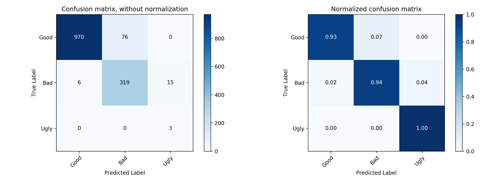
Figure 5: Left: Confusion Matrix for the test set; Right: Confusion Matrix with normalization.

5 Conclusion

In this work, we examine the application of deep learning to perform a quality classifier of shot-gather noisy images. For that sake, we build a dataset with $6,613$ seismic shot-gather images and manually classified them using good, bad and ugly labels, according to a visual inspection of artifacts related to swell noise and anomalous recorded amplitude. We propose the Minception Net, a network architecture inspired on GoogleNet’s Inception Block, but with fewer parameters. Additionally, we also propose three Minception variants that incorporate mechanisms as residual connection (Residual Minception), attention (Attention Minception) and squeeze-and-excitation (SE-Minception).

In a 10-fold cross validation experiment, we use as baseline three CNNs InceptionV3, VGG16 and VGG19 to extract features from shot-gather images and apply their values as the input of an SVM classifier. The best result is obtained by the second block from VGG19 with an F1-W of 90.82%. The SE-Minception variant achieves the best result with an F1-W of 93.84% . Then, we optimize SE-MinceptionNet by performing a $\alpha$ search, where $\alpha$ is a parameter that multiplies the quantity of initial kernels from the standard minception block. With this search, we are looking for a balance between the depth and the width of the network. The validation results show that setting alpha to 8 upgrades the F1-W to 94.91%. In the test set, the SE-MinceptionNet produced a final F1-W of 93.5%.

As future work, we plan to use deep learning models for data augmentation to increase the quantity of ugly seismic shot-gather images in training. We expect this will produce a reliable recall and improve the value of F1-score for ugly label.

References

- [1] Leonardo T Duarte, Daniela Donno, Renato R Lopes, and Joao Marcos T Romano. Seismic signal processing: Some recent advances. In 2014 IEEE International Conference on Acoustics, Speech and Signal Processing (ICASSP), pages 2362–2366. IEEE, 2014.
- [2] Öz Yilmaz. Seismic data analysis: Processing, inversion, and interpretation of seismic data. Society of exploration geophysicists, 2001.
- [3] Andrew P Valentine and John H Woodhouse. Approaches to automated data selection for global seismic tomography. Geophysical Journal International, 182(2):1001–1012, 2010.
- [4] Prateek Jain, Brian Kulis, Jason V. Davis, and Inderjit S. Dhillon. Metric and kernel learning using a linear transformation. Journal of Machine Learning Research, 13, 10 2009.
- [5] Ian McBrearty, Andrew Delorey, and Paul A. Johnson. Pairwise association of seismic arrivals with convolutional neural networks. Seismological Research Letters, 90, 01 2019.
- [6] Elad Hoffer and Nir Ailon. Deep metric learning using triplet network, 2014.
- [7] Bernhard E Boser, Isabelle M Guyon, and Vladimir N Vapnik. A training algorithm for optimal margin classifiers. In Proceedings of the fifth annual workshop on Computational learning theory, pages 144–152. ACM, 1992.
- [8] Thomas Elboth, Fugro Geoteam, and Dag Hermansen. Attenuation of noise in marine seismic data. In SEG Technical Program Expanded Abstracts 2009, pages 3312–3316. Society of Exploration Geophysicists, 2009.
- [9] Christian Szegedy, Wei Liu, Yangqing Jia, Pierre Sermanet, Scott Reed, Dragomir Anguelov, Dumitru Erhan, Vincent Vanhoucke, and Andrew Rabinovich. Going deeper with convolutions. In Proceedings of the IEEE conference on computer vision and pattern recognition, pages 1–9, 2015.
- [10] Kaiming He, Xiangyu Zhang, Shaoqing Ren, and Jian Sun. Deep residual learning for image recognition. 2016 IEEE Conference on Computer Vision and Pattern Recognition (CVPR), pages 770–778, 2016.
- [11] Sanghyun Woo, Jongchan Park, Joon-Young Lee, and In-So Kweon. Cbam: Convolutional block attention module. In ECCV, 2018.
- [12] J. Hu, L. Shen, and G. Sun. Squeeze-and-excitation networks. In IEEE Conference on Computer Vision and Pattern Recognition, 2018.
- [13] Karen Simonyan and Andrew Zisserman. Very deep convolutional networks for large-scale image recognition. arXiv preprint arXiv:1409.1556, 2014.
- [14] Christian Szegedy, Vincent Vanhoucke, Sergey Ioffe, Jon Shlens, and Zbigniew Wojna. Rethinking the inception architecture for computer vision. In Proceedings of the IEEE conference on computer vision and pattern recognition, pages 2818–2826, 2016.
- [15] Jia Deng, Wei Dong, Richard Socher, Li-Jia Li, Kai Li, and Li Fei-Fei. Imagenet: A large-scale hierarchical image database. 2009.
- [16] Jason Yosinski, Jeff Clune, Anh Nguyen, Thomas Fuchs, and Hod Lipson. Understanding neural networks through deep visualization. arXiv preprint arXiv:1506.06579, 2015.