High Scale Validity of the DFSZ Axion Model with Precision

Abstract

With the assumption of classical scale invariance at the Planck scale, the DFSZ axion model can generate the Higgs mass terms of the appropriate size through technically natural parameters and may be valid up to the Planck scale. We discuss the high scale validity of the Higgs sector, namely the absence of Landau poles and the vacuum stability. The Higgs sector is identical to that of the type-II two Higgs doublet model with a limited number of the Higgs quartic couplings. We utilize the state-of-the-art method to calculate vacuum decay rates and find that they are enhanced at most by $10^{10}$ compared with the tree level evaluation. We also discuss the constraints from flavor observables, perturbative unitarity, oblique parameters and collider searches. We find that the high scale validity tightly constrains the parameter region, but there is still a chance to observe at most about $10\%$ deviation of the $125~{}{\rm GeV}$ Higgs couplings to the fermions.

I Introduction

An invisible axion Peccei and Quinn (1977); Weinberg (1978); Wilczek (1978); Abbott and Sikivie (1983); Dine and Fischler (1983); Preskill et al. (1983); Kuster et al. (2008); Shifman et al. (1980); Kim (1979); Zhitnitsky (1980); Dine et al. (1981) is one of the plausible solutions to the strong CP problem and is also an excellent dark matter candidate. We focus on the DFSZ axion model Zhitnitsky (1980); Dine et al. (1981), where the standard model (SM) is extended with a SM singlet complex scalar and an additional Higgs doublet. Since the Higgs doublets have non-zero Peccei-Quinn (PQ) charges, the Higgs couplings are tightly restricted by the PQ symmetry. For example, dangerous flavor changing neutral currents (FCNC) are forbidden at the tree level and the CP is not broken spontaneously in the scalar sector.

In this paper, we discuss the possibility that the DFSZ axion model remains valid up to the Planck scale. In such a scenario, one of the disadvantages is that we need to give up a complete explanation of the hierarchy between the Planck scale and the electroweak (EW) scale. However, if there is a mechanism that realizes classical scale invariance at the Planck scale, the hierarchy problem may be solved without introducing supersymmetry or compositeness Bardeen (1995); Hill (2005); Aoki and Iso (2012). Since the scale invariance is violated at the quantum level, the PQ breaking scale can appear through the dimensional transmutation. If the PQ sector and the Higgs sector are connected by (technically natural) tiny couplings, the PQ breaking can also generate the Higgs mass terms without causing a hierarchy problem Allison et al. (2015, 2014). Since the PQ breaking sector decouples from the Higgs sector due to the tiny couplings, the model is well approximated by the type-II two Higgs doublet model (THDM) with a restricted number of coupling constants. Importantly, the additional Higgs bosons should be around the EW scale in this scenario since there is no technically natural parameter that accommodates a hierarchy among the Higgs boson masses.

Another disadvantage is that the model does not explain the neutrino masses, the baryon asymmetry of the Universe, or inflation. However, they can be explained without affecting the Higgs sector. For example, one may consider the see-saw mechanism with right handed neutrinos having a few orders of magnitude smaller masses than the PQ breaking scale Vissani (1998); Farina et al. (2013); Foot et al. (2014). It can explain the neutrino masses and also the baryon asymmetry of the Universe with $\tan\beta\gtrsim 4$ Clarke et al. (2015). However, it does not cause the hierarchy problem thanks to the tiny Yukawa couplings of the right handed neutrinos. As for inflation, one may attach an inflation sector to the model and assume tiny couplings between the inflation sector and the Higgs sector, which is, at least, technically natural.

For the model to be valid up to the Planck scale, Landau poles should not appear during the renormalization group (RG) evolution and the lifetime of the EW vacuum should be long enough. We refer to these two conditions as the high scale validity. Similar discussions can be found in the context of THDMs Branchina et al. (2018); Krauss et al. (2018); Basler et al. (2018); Chakrabarty and Mukhopadhyaya (2017a, b); Cacchio et al. (2016); Bagnaschi et al. (2016); Chowdhury and Eberhardt (2015); Ferreira et al. (2015); Das and Saha (2015); Chakrabarty et al. (2014); Grzadkowski et al. (2014); Shu and Zhang (2013). As we will see and as found in the previous studies, these conditions are complementary and become very restrictive if combined. Thus, the model becomes more predictive and it is important to determine the allowed parameter space precisely.

The lifetime of the EW vacuum is estimated by the bubble nucleation rate Coleman (1977); Callan and Coleman (1977), which has a form of

$$\gamma=\mathcal{A}e^{-\mathcal{B}},$$ (1)

where $\mathcal{B}$ is the Euclidean action of the so-called the bounce, and $\mathcal{A}$ represents quantum corrections to $\mathcal{B}$ having mass dimension four. In many papers, $\mathcal{A}$ is assumed to lie around the typical scale of the problem, but it has been pointed out Endo et al. (2016) that such an estimation leads to theoretical uncertainty of $e^{-\mathcal{B}\times\mathcal{O}(10\%)}$ in the nucleation rate. As we will see later, it can become comparable with the uncertainties coming from those of the top mass and the strong coupling. Thus, it is important to calculate both of $\mathcal{A}$ and $\mathcal{B}$ to get a precise vacuum decay rate.

The one-loop calculation of $\mathcal{A}$ for the SM was first calculated in Isidori et al. (2001). Since the treatment of the gauge zero mode had not been known at that time, the calculation was not complete. Recently, the correct treatment has been found Endo et al. (2017) and the one-loop calculation for the SM has been completed Andreassen et al. (2018); Chigusa et al. (2017, 2018). In addition, the analytic expression for $\mathcal{A}$ at the one-loop level has become available Andreassen et al. (2018); Chigusa et al. (2018) for an approximately scale invariant theory. Since they are applicable to the case where the bounce is composed of a single field, we extend them to a multi-field case in this paper. Differently from the single-field case, there can be more than one unstable directions and there can appear an additional zero mode due to a global symmetry breaking. In addition, the electromagnetic $U(1)$ symmetry can also be broken spontaneously.

Before the analysis of the high scale validity, we impose the constraints from flavor observables, perturbative unitarity, oblique parameters and collider searches. For the constraints from flavor observables, we obtain the $95\%$ exclusion limit in Appendix A using the recent experimental values.

We determine the allowed parameter space by utilizing the Monte Carlo method. We show how much the high scale validity narrows down the parameter space and discuss the implications on the Higgs couplings and the Higgs mass splittings.

This paper is organized as follows. In Section II, we briefly explain the DFSZ axion model. Section III is devoted to the details of the analysis on the bubble nucleation rate for the multi-field case. Then, in Section IV, we discuss the low energy constraints. In Section V, we execute numerical analysis and discuss the consequence of the high scale validity. Finally, we summarize in Section VI.

II DFSZ Axion Model

In this section, we briefly review the DFSZ axion model Zhitnitsky (1980); Dine et al. (1981). The scalar sector consists of two Higgs doublets, $H_{1}$ and $H_{2}$, and a SM singlet complex scalar, $\Phi$. We choose the PQ charges of $H_{1}$, $H_{2}$ and $\Phi$ to be $x_{1}$, $x_{2}$ and $(x_{2}-x_{1})/2$, respectively. Here, we assume $x_{1}\neq x_{2}$ so that $\Phi$ has a non-zero PQ charge.

The general scalar potential is given by

$$V(H_{1},H_{2},\Phi) =\tilde{m}_{1}^{2}H_{1}^{\dagger}H_{1}+\tilde{m}_{2}^{2}H_{2}^{\dagger}H_{2}+\frac{\lambda_{1}}{2}(H_{1}^{\dagger}H_{1})^{2}+\frac{\lambda_{2}}{2}(H_{2}^{\dagger}H_{2})^{2}$$

$$\hskip 12.91663pt+\lambda_{3}(H_{1}^{\dagger}H_{1})(H_{2}^{\dagger}H_{2})+\lambda_{4}(H_{1}^{\dagger}H_{2})(H_{2}^{\dagger}H_{1})$$

$$\hskip 12.91663pt+\tilde{\lambda}_{\Phi}(|\Phi|^{2}-v_{\Phi}^{2})^{2}$$

$$\hskip 12.91663pt+|\Phi|^{2}(\tilde{\kappa}_{1}H_{1}^{\dagger}H_{1}+\tilde{\kappa}_{2}H_{2}^{\dagger}H_{2})-(\tilde{\kappa}_{3}\Phi^{2}H_{2}^{\dagger}H_{1}+h.c.),$$ (2)

where $v_{\Phi}^{2}$, $\tilde{m}_{i}^{2}$’s, $\lambda_{i}$’s, $\tilde{\lambda}_{\Phi}$ and $\tilde{\kappa}_{i}$’s are constants. We assume $\tilde{\lambda}_{\Phi}$ is moderate so that the VEV of $\Phi$ is not affected by those of $H_{1}$ and $H_{2}$.

We assume the classical scale invariance and set $\tilde{m}_{1}^{2}$ and $\tilde{m}_{2}^{2}$ to zero at the Planck scale. Then, the Higgs mass terms are assumed to be generated through the PQ symmetry breaking. In order to obtain the EW scale, $\tilde{\kappa}_{i}$’s should be very small since $\Phi$ has to develop a huge vacuum expectation value (VEV) to avoid the constraints on the axion decay constant, $10^{9}~{}{\rm GeV}\lesssim f_{a}\lesssim 10^{12}~{}{\rm GeV}$ Peccei (2008); Turner (1990). Due to the smallness of $\tilde{\kappa}_{i}$’s, $\Phi$ decouples from the Higgs sector and the potential reduces to

$$V_{\rm THDM} =m_{1}^{2}H_{1}^{\dagger}H_{1}+m_{2}^{2}H_{2}^{\dagger}H_{2}-(m_{3}^{2}H_{2}^{\dagger}H_{1}+h.c.)+\frac{\lambda_{1}}{2}(H_{1}^{\dagger}H_{1})^{2}$$

$$\hskip 12.91663pt+\frac{\lambda_{2}}{2}(H_{2}^{\dagger}H_{2})^{2}+\lambda_{3}(H_{1}^{\dagger}H_{1})(H_{2}^{\dagger}H_{2})+\lambda_{4}(H_{1}^{\dagger}H_{2})(H_{2}^{\dagger}H_{1}),$$ (3)

where

$$m_{1}^{2} =\tilde{\kappa}_{1}v_{\Phi}^{2},$$ (4)

$$m_{2}^{2} =\tilde{\kappa}_{2}v_{\Phi}^{2},$$ (5)

$$m_{3}^{2} =|\tilde{\kappa}_{3}|v_{\Phi}^{2}.$$ (6)

Here, we took $m_{3}^{2}$ to be real and positive by the redefinition of the phase of $H_{1}$. Notice that PQ violating quartic couplings can be generated after the PQ symmetry breaking, but they are suppressed by $\tilde{\kappa}_{i}$’s and hence are negligible.

With the PQ charge assignment shown in Table 1, the Higgs doublets couple to the SM fermions as

$$\mathcal{L}_{\rm Yukawa}=-y_{U}\bar{Q}\tilde{H}_{2}U-y_{D}\bar{Q}H_{1}D-y_{E}\bar{L}H_{1}E+h.c.,$$ (7)

with

$$\tilde{H}_{2}=i\sigma_{2}H_{2}^{*}.$$ (8)

Here, $i\sigma_{2}$ is the completely anti-symmetric matrix and $Q$, $L$, $U$, $D$ and $E$ represent the left quark doublets, the left lepton doublets, the up-type quarks, the down-type quarks and the charged leptons in the SM, respectively. The model is thus regarded as the type-II THDM with a limited number of Higgs quartic couplings.

PQ Charge Assignment
$H_{1}$	$H_{2}$	$\Phi$	$Q$	$L$	$U$	$D$	$E$
$x_{1}$	$x_{2}$	$\frac{x_{2}-x_{1}}{2}$	$0$	$0$	$x_{2}$	$-x_{1}$	$-x_{1}$

Table 1: Assignment of the PQ charge in the DFSZ axion model.

Let us define the mass eigenstates and the mixing angles. We expand the Higgs fields as

$$H_{j}=\begin{pmatrix}\omega_{j}^{+}\\ (v_{j}+h_{j}-i\zeta_{j})/\sqrt{2}\end{pmatrix},$$ (9)

with

$$\begin{pmatrix}h_{1}\\ h_{2}\end{pmatrix}=R(\alpha)\begin{pmatrix}H\\ h\end{pmatrix},~{}\begin{pmatrix}\zeta_{1}\\ \zeta_{2}\end{pmatrix}=R(\beta)\begin{pmatrix}G^{0}\\ A\end{pmatrix},~{}\begin{pmatrix}\omega_{1}^{+}\\ \omega_{2}^{+}\end{pmatrix}=R(\beta)\begin{pmatrix}G^{+}\\ H^{+}\end{pmatrix},$$ (10)

where $v_{i}$’s are the VEVs of the Higgs fields, $\tan\beta=v_{2}/v_{1}$ and

$$R(\theta)=\begin{pmatrix}\cos\theta&-\sin\theta\\ \sin\theta&\cos\theta\end{pmatrix}.$$ (11)

Here, $h$ is the $125~{}{\rm GeV}$ Higgs boson, $H$ is the additional CP-even Higgs boson, $A$ is the CP-odd Higgs boson, $H^{+}$ is the charged Higgs boson, and $G^{0}$ and $G^{+}$ are the would-be Nambu-Goldstone bosons. The SM-like limit for $h$ is given by $\beta-\alpha\to\pi/2$.

III Vacuum Decay Rate

Since the quantum corrections to the effective potential depend on the VEVs of the Higgs fields, the shape of the effective potential is non-trivial at large Higgs VEVs. When there is a deeper vacuum or the effective potential is unbounded from below, the EW vacuum is not absolutely stable and decays through quantum tunneling. Even in such a case, we can live in the meta-stable vacuum if it has a much longer lifetime than the age of the Universe. In this section, we discuss the precise determination of vacuum decay rates for the DFSZ axion model.

III.1 Formulation

Recently, the analytic formulas for the prefactor, $\mathcal{A}$, at the one-loop level have been derived Andreassen et al. (2018); Chigusa et al. (2018), which are applicable to the case where the theory is approximately scale invariant and the bounce consists of a single field. In the following, we extend their results to the case where the bounce consists of more than one fields.

Since the PQ-breaking sector couples to the THDM sector very weakly, the vacuum decay rate can be calculated independently of the PQ-breaking sector, i.e. the decay path, the RG running or the calculation of $\mathcal{A}$ is not affected by the PQ-breaking sector. Notice that even when the field value of $H_{1}$ or $H_{2}$ becomes much larger than the PQ-breaking scale, $\Phi$ is almost constant during the tunneling. This is because the typical size of a bounce, i.e. $\bar{R}\simeq 1/\sqrt{|H_{1}(0)|^{2}+|H_{2}(0)|^{2}}$, is too small. Here, $H_{i}(0)$’s are the field values at the center of the bounce. For example, let us assume that $\Phi$ obtains a negative mass squared, $m_{\Phi}^{2}<0$, during the tunneling. Then, the displacement of $\Phi$ is roughly estimated as $v_{\Phi}(e^{\sqrt{|m_{\Phi}^{2}|}\bar{R}}-1)$, which is negligible since $|m_{\Phi}^{2}|\ll 1/\bar{R}^{2}$.

Since the field value at the true vacuum is typically much larger than the EW scale, the Higgs potential is approximately given by

$$V_{\rm THDM} \simeq\frac{\lambda_{1}}{2}(H_{1}^{\dagger}H_{1})^{2}+\frac{\lambda_{2}}{2}(H_{2}^{\dagger}H_{2})^{2}+\lambda_{3}(H_{1}^{\dagger}H_{1})(H_{2}^{\dagger}H_{2})+\lambda_{4}(H_{1}^{\dagger}H_{2})(H_{2}^{\dagger}H_{1}).$$ (12)

For the moment, we fix the renormalization scale and will discuss the running effect later.

The bounce is a solution to the Euclidean equations of motion that are given by

$$\frac{d^{2}H_{1}^{i}}{dr^{2}}+\frac{3}{r}\frac{dH_{1}^{i}}{dr} =\frac{\partial V_{\rm THDM}}{\partial H_{1}^{i*}},$$ (13)

$$\frac{d^{2}H_{2}^{i}}{dr^{2}}+\frac{3}{r}\frac{dH_{2}^{i}}{dr} =\frac{\partial V_{\rm THDM}}{\partial H_{2}^{i*}},$$ (14)

with boundary conditions,

$$\frac{dH_{1}^{i}}{dr}(0)=\frac{dH_{2}^{i}}{dr}(0)=0,~{}H_{1}^{i}(\infty)=H_{2}^{i}(\infty)=0,$$ (15)

and their complex conjugates. Here, $r$ is the radius from the center of the bubble and $i=1,2$ labels the components of the doublet. Without loss of generality, we parameterize the Higgs fields as

$$H_{1}=\frac{1}{\sqrt{2}}\begin{pmatrix}0\\ \phi\cos\Omega\end{pmatrix},~{}H_{2}=\frac{1}{\sqrt{2}}e^{i(\sigma_{1}\theta_{1}+\sigma_{2}\theta_{2})}e^{i\sigma_{3}\theta_{3}}\begin{pmatrix}0\\ \phi\sin\Omega\end{pmatrix},$$ (16)

where $\sigma_{i}$’s are the Pauli matrices. Then, the potential is expressed as

$$V_{\rm THDM}\simeq\frac{\lambda_{\phi}(\Omega,\Theta)}{4}\phi^{4},$$ (17)

where

$$\lambda_{\phi}(\Omega,\Theta) =\frac{1}{2}\left[\lambda_{1}\cos^{4}\Omega+\lambda_{2}\sin^{4}\Omega+2(\lambda_{3}+\lambda_{4}\cos^{2}\Theta)\sin^{2}\Omega\cos^{2}\Omega\right],$$ (18)

$$\Theta =\sqrt{\theta_{1}^{2}+\theta_{2}^{2}}.$$ (19)

In Appendix B, we show that $\Omega$ and $\Theta$ are constant. Then, the equations of motion reduce to

$$\frac{\partial\lambda_{\phi}}{\partial\Theta} =0,$$ (20)

$$\frac{\partial\lambda_{\phi}}{\partial\Omega} =0,$$ (21)

$$\frac{d^{2}\phi}{dr^{2}}+\frac{3}{r}\frac{d\phi}{dr} =\lambda_{\phi}\phi^{3},$$ (22)

with boundary conditions

$$\frac{d\phi}{dr}(0)=0,~{}\phi(\infty)=0.$$ (23)

From Eq. (18), we can see that a minimum of $\lambda_{\phi}$ satisfies $\cos^{2}\Theta=0$ for $\lambda_{4}\geq 0$, and $\cos^{2}\Theta=1$ for $\lambda_{4}<0$. Then, from Eq. (21), we get the following solutions;

$$(a) ~{}\Omega=0,~{}\lambda_{\phi}=\frac{1}{2}\lambda_{1},$$ (24)

$$(b) ~{}\Omega=\frac{\pi}{2},~{}\lambda_{\phi}=\frac{1}{2}\lambda_{2},$$ (25)

$$(c) ~{}\tan^{2}\Omega=\frac{\lambda_{1}-\bar{\lambda}}{\lambda_{2}-\bar{\lambda}},~{}\lambda_{\phi}=\frac{1}{2}\frac{\lambda_{1}\lambda_{2}-\bar{\lambda}^{2}}{\lambda_{1}+\lambda_{2}-2\bar{\lambda}},$$ (26)

where

$$\bar{\lambda}=\min(\lambda_{3},\lambda_{3}+\lambda_{4}).$$ (27)

Notice that $(c)$ exists only when $(\lambda_{1}-\bar{\lambda})/(\lambda_{2}-\bar{\lambda})>0$.

If $\lambda_{\phi}<0$, the solution to Eqs. (22) and (23) is given by

$$\phi(r)=\sqrt{\frac{8}{|\lambda_{\phi}|}}\frac{R}{R^{2}+r^{2}},$$ (28)

which gives

$$\mathcal{B}=\frac{8\pi^{2}}{3|\lambda_{\phi}|},$$ (29)

with $R$ being a free parameter that fixes the radius of the bounce. Notice that $\mathcal{B}$ is independent of $R$, which is due to the (approximate) classical scale invariance.

Since all the possible bounces contribute to the vacuum decay rate, the total vacuum decay rate is expressed as

$$\gamma=\sum_{\lambda_{\phi}}\int dR\frac{d\gamma}{dR},$$ (30)

where $\lambda_{\phi}$ is summed over its minima with $\lambda_{\phi}<0$. Now, the problem is reduced to the single field case for each $\lambda_{\phi}$ and we can use the one-loop results of Andreassen et al. (2018); Chigusa et al. (2017, 2018). The details are in Appendix C.

Let us discuss the convergence of the $R$ integral. From the dimensional analysis and the renormalization scale independence of the vacuum decay rate, the $R$-dependence of the integrand can be determined as

$$\frac{d\gamma}{dR}\propto R^{-5}(\mu R)^{-\frac{8\pi^{2}\beta_{\lambda_{\phi}}^{(1)}}{3\lambda_{\phi}^{2}}},$$ (31)

at the one-loop level. Here, $\mu$ is the renormalization scale and $\beta_{\lambda_{\phi}}^{(1)}$ is the one-loop beta function for $\lambda_{\phi}$. Thus, if we integrate it over $R\in(0,\infty)$, the integration does not converge. However, as discussed in Andreassen et al. (2018); Chigusa et al. (2017, 2018), the result can be convergent if we include higher-loop corrections. Although it is very difficult to calculate them, their $R$-dependence is completely determined by the beta functions and we can sum up the logarithmic corrections by taking $\mu\sim 1/R$ for each bounce with radius $R$ (for detailed discussion see Chigusa et al. (2018)). If there exists a minimum of the effective action, it dominates the $R$ integral and the result is convergent.

Independently of the convergence of the $R$ integral, we use cut-offs for the $R$ integral for the following reasons. First, we need an IR cut-off because we have ignored the dimensionful couplings. Second, we need a UV cut-off because we do not consider gravitational corrections. Thus, we set the integration region as

$$\gamma=\sum_{\lambda_{\phi}}\int_{1/M_{\rm Pl}}^{1/(10~{}{\rm TeV})}dR\frac{d\gamma}{dR},$$ (32)

where $M_{\rm Pl}$ is the reduced Planck scale. We also impose the same limits on the field value of the bounce as

$$10~{}{\rm TeV}\lesssim\phi(0)=\sqrt{\frac{8}{|\lambda_{\phi}(\mu)|}}\frac{1}{R}\lesssim M_{\rm Pl},$$ (33)

when $\lambda_{\phi}<0$.

We also exclude the region where the quantum corrections to the action become larger than $80\%$ of $\mathcal{B}$ since the perturbative expansions become unreliable. Such a region appears where $\lambda_{\phi}$ is very close to zero.

Since the integrand of the vacuum decay rate is positive definite, these limits always make the vacuum decay rate small. Thus, what we get with these limits is a lower bound on the vacuum decay rate and it always gives a conservative constraint.

The condition for the stability of the EW vacuum is then given by

$$\gamma\lesssim H_{0}^{4},$$ (34)

where $H_{0}\simeq 67.66~{}{\rm(km/s)/Mpc}$ Aghanim et al. (2018) is the current Hubble constant.

III.2 Example

Let us show an example of the calculation. We take

$$\tan\beta=9,~{}\cos(\beta-\alpha)=0.0004,$$

$$m_{H}=602.5~{}{\rm GeV},~{}m_{A}=602.5~{}{\rm GeV},~{}m_{H^{+}}=600~{}{\rm GeV}.$$ (35)

We first calculate the ${\rm\overline{MS}}$ dimensionless couplings at renormalization scale $\mu_{t}=m_{t}$, where we include the one-loop corrections and the four-loop QCD corrections. The details are in Appendix D. Then, we evolve them with the two-loop RG equations. The result is shown in the top left panel of Fig. 1. In this example, only $\lambda_{2}$ becomes negative and contributes to the vacuum decay rate.

Next, we calculate the differential vacuum decay rate, $d\gamma/d(\ln R)$, for case (b). We take $\mu=1/R$. The result is shown with the solid line in the top right panel of Fig. 1. Integrating it over $\ln R$, we get

$$\log_{10}[\gamma\times{\rm Gyr}~{}{\rm Gpc}^{3}]=-3.5^{~{}+21.7~{}+11.0~{}+1.4~{}+0.1}_{~{}-26.1~{}-11.8~{}-1.5~{}-0.3},$$ (36)

where the 1st, 2nd, 3rd and 4th errors are those from $m_{t}$, $\alpha_{s}$, $m_{h}$ and $\mu$, respectively. We use the SM values and uncertainties given in Table 3 and $\alpha_{s}=0.1181(11)$. We estimate the renormalization scale uncertainty by taking $\mu=2/R$ and $\mu=1/(2R)$. With this parameter set, the vacuum decay rate is close to the upper bound, $\log_{10}[H_{0}^{4}\times{\rm Gyr}~{}{\rm Gpc}^{3}]\simeq-3$.

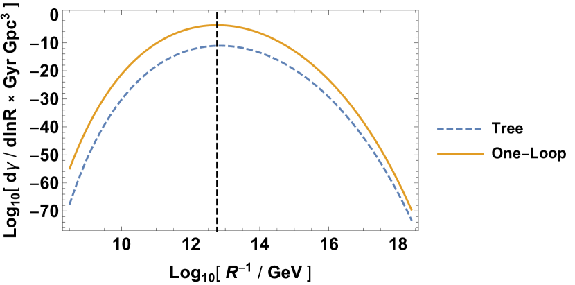
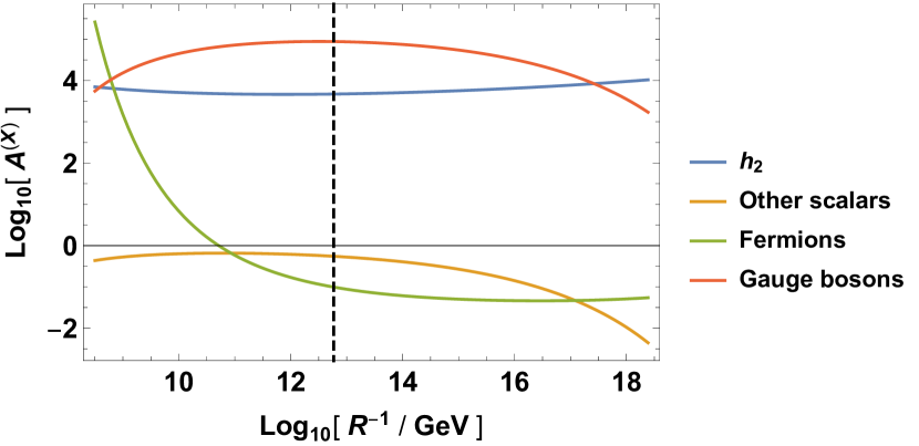
Figure 1: An example of the calculation of a vacuum decay rate. The top left panel shows the RG evolution of the Higgs quartic couplings. The top right panel shows the differential vacuum decay rates with and without the calculation of $\mathcal{A}$. The bottom panel shows each quantum correction to the differential vacuum decay rate. The vertical black dashed line indicates the maximum of the differential vacuum decay rate.

Let us see the difference between the “tree level” vacuum decay rate and our result. For the tree level vacuum decay rate, we adopt

$$\gamma_{\rm tree}=\max_{R,\lambda_{\phi}}\left[\frac{1}{R^{4}}e^{-\frac{8\pi^{2}}{3|\lambda_{\phi}|}}\right]_{\mu=R^{-1}},$$ (37)

where the maximum value is searched in the same region as the integration region of the one-loop vacuum decay rate. In the top right panel of Fig. 1, we show $R^{-4}\exp[-8\pi^{2}/(3|\lambda_{\phi}|)]$ with the dashed line. We get

$$\log_{10}[\gamma_{\rm tree}\times{\rm Gyr}~{}{\rm Gpc}^{3}]=-11.2.$$ (38)

Thus, the one-loop calculation enhances the vacuum decay rate by about $10^{7.7}$. We show each quantum contribution in the bottom panel of Fig. 1. The vertical black dashed line corresponds to the maximum of the differential vacuum decay rate. Around the maximum, the gauge bosons and $h_{2}$ have positive contributions and the fermions and the other scalars have negative contributions. The former contributions are larger than the latter and the positive contribution remains.

In Fig. 2, we show the binned plot of the vacuum decay rates at the tree level and at the one-loop level by using the data accumulated for Fig. 4. We observe that the enhancement of the vacuum decay rate is generic for $\gamma\gtrsim H_{0}^{4}$ and that it is enhanced at most by $10^{10}$, which is comparable with the uncertainties from those of the top mass and the strong coupling constant. For $\gamma\ll H_{0}^{4}$, the vacuum decay rate can be either suppressed or enhanced.

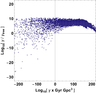
Figure 2: The difference between the tree level vacuum decay rates and the one-loop level vacuum decay rates. We use the data accumulated for Fig. 4. We show only $-200\lesssim\log_{10}[\gamma\times{\rm Gyr}{\rm Gpc}^{3}]\lesssim 200$.

IV Low Energy Constraints

Before the discussion of the high scale validity, let us discuss the low energy constraints; flavor observables, perturbative unitarity, oblique parameters, and collider searches. In this section, we do not consider the constraints from the signal strengths of the $125~{}{\rm GeV}$ Higgs boson since they are the outputs of our analysis.

IV.1 Flavor Observables

The additional Higgs bosons contribute to flavor observables and the current strongest constraints for the type-II THDM come from the branching ratios of $B\to\tau\nu$, $B_{s}\to\mu\mu$ and $b\to s\gamma$, and the $B_{s}-\bar{B}_{s}$ mixing as discussed, for example, in Arbey et al. (2018); Misiak and Steinhauser (2017); Haller et al. (2018). We obtain the constraints following the analysis of Enomoto and Watanabe (2016) with the current experimental values. The details are given in Appendix A.

In Fig. 3, we plot the $95\%$ exclusion limits on the $(m_{H^{+}},\tan\beta)$-plane with assuming $m_{H}=m_{A}=m_{H^{+}}$ and $\cos(\beta-\alpha)=0$. The white region is allowed and the shaded regions are excluded by the observables shown on the regions. As we can see, ${\rm BR}(b\to s\gamma)$ gives the lower bound of $m_{H^{+}}\gtrsim 580~{}{\rm GeV}$ almost independently of $\tan\beta$. The upper bound and the lower bound on $\tan\beta$ are set by ${\rm BR}(B_{s}\to\mu\mu)$ and $\Delta M_{B_{s}}$, respectively. Notice that these constraints are stronger than the perturbativity limits of $y_{t},y_{b}\lesssim\sqrt{4\pi}$. The results are consistent with the recent works Arbey et al. (2018); Misiak and Steinhauser (2017); Haller et al. (2018).

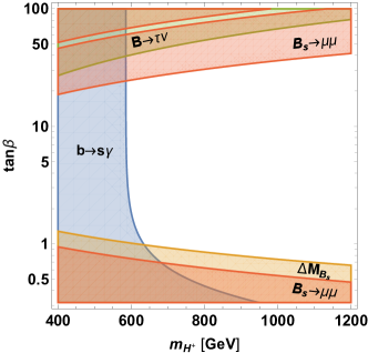
Figure 3: The $95\%$ CL constraints from flavor observables. The blue, the orange, the red, and the green shaded regions are excluded by ${\rm BR(b\to s\gamma)}$, $\Delta M_{B_{s}}$, ${\rm BR}(B_{s}\to\mu\mu)$, and ${\rm BR}(B\to\tau\nu)$, respectively.

IV.2 Low Energy Perturbative Unitarity

For the study of the high scale validity, the perturbative unitarity is necessary because otherwise all the calculations, including the matching conditions to the ${\rm\overline{MS}}$ couplings, become unreliable.

At the tree level, the Higgs quartic couplings are related to the Higgs masses and mixing as

$$\lambda_{1} =\frac{1}{2v^{2}\cos^{2}\beta}\left[m_{h}^{2}+m_{H}^{2}-(1-\cos 2\beta)m_{A}^{2}+(m_{H}^{2}-m_{h}^{2})\cos 2\alpha\right],$$ (39)

$$\lambda_{2} =\frac{1}{2v^{2}\sin^{2}\beta}\left[m_{h}^{2}+m_{H}^{2}-(1+\cos 2\beta)m_{A}^{2}-(m_{H}^{2}-m_{h}^{2})\cos 2\alpha\right],$$ (40)

$$\lambda_{3} =\frac{1}{v^{2}}\left[2m_{H^{+}}^{2}-m_{A}^{2}+(m_{H}^{2}-m_{h}^{2})\frac{\sin 2\alpha}{\sin 2\beta}\right],$$ (41)

$$\lambda_{4} =\frac{2}{v^{2}}(m_{A}^{2}-m_{H^{+}}^{2}).$$ (42)

Then, we impose the condition of the $s$-wave unitarity, which is given by Kanemura et al. (1993); Akeroyd et al. (2000)

$$|\lambda_{1}| <8\pi,$$ (43)

$$|\lambda_{2}| <8\pi,$$ (44)

$$|\lambda_{3}| <8\pi,$$ (45)

$$|\lambda_{3}\pm\lambda_{4}| <8\pi,$$ (46)

$$|\lambda_{3}+2\lambda_{4}| <8\pi,$$ (47)

$$\left|\frac{1}{2}\left(\lambda_{1}+\lambda_{2}\pm\sqrt{(\lambda_{1}-\lambda_{2})^{2}+4\lambda_{4}^{2}}\right)\right| <8\pi,$$ (48)

$$\left|\frac{3}{2}\left(\lambda_{1}+\lambda_{2}\pm\sqrt{(\lambda_{1}-\lambda_{2})^{2}+\frac{4}{9}(2\lambda_{3}+\lambda_{4})^{2}}\right)\right| <8\pi,$$ (49)

at the tree level. Since we will use the same condition to detect Landau poles later, we refer to the perturbative unitarity with the tree level matching conditions as “the low energy (LE) perturbative unitarity”.

IV.3 Oblique Parameters

The oblique parameters, especially the $S$-parameter and the $T$-parameter, are affected by the additional Higgs doublet. We use the general formulas for multi-Higgs-doublet models Grimus et al. (2008a, b) (for the THDM, see Eriksson et al. (2010)) to calculate these parameters.

The current constraints are given by Tanabashi et al. (2018)

$$S =0.02\pm 0.07,$$ (50)

$$T =0.06\pm 0.06,$$ (51)

with the assumption of $U=0$. The correlation coefficient is $\rho=0.92$. We adopt $95\%$ exclusion limit on $S$ and $T$, which is given by

$$\chi^{2}_{2\,{\rm dof}}\equiv\frac{1}{1-\rho^{2}}\left[\frac{(S-S_{\rm cent})^{2}}{\sigma_{S}^{2}}+\frac{(T-T_{\rm cent})^{2}}{\sigma_{T}^{2}}-2\rho\frac{(S-S_{\rm cent})(T-T_{\rm cent})}{\sigma_{S}\sigma_{T}}\right]<5.99,$$ (52)

where $S_{\rm cent}$ and $T_{\rm cent}$ are the central values of $S$ and $T$, respectively.

IV.4 Collider Searches

New scalar particles have been searched extensively at Tevatron, LEP and LHC. We utilize HiggsBounds Bechtle et al. (2014, 2012, 2011, 2010, 2015) to check the constraints from the collider searches. For simplicity, we consider only on-shell decays for non-SM channels. The couplings and the partial decay widths used in the analysis are summarized in Appendix F.

V High Scale Validity

At an energy scale much higher than the EW scale, the model becomes classically scale invariant and only the dimensionless couplings become relevant. We first match the $\overline{\rm MS}$ couplings at the one-loop level, where the matching scale is taken to the top mass scale. For the top and the bottom Yukawa couplings, we also include the four-loop QCD corrections. Then, we evolve the dimensionless couplings up to the Plank scale using the two-loop beta functions. In these calculations, we utilize the public codes of SARAH Staub et al. (2012); Staub (2015), FeynArts Hahn (2001), FeynCalc Mertig et al. (1991); Shtabovenko et al. (2016), and RunDec Chetyrkin et al. (2000); Herren and Steinhauser (2018). The details of the matching conditions are given in Appendix D. Throughout this analysis, we adopt the central values for the SM inputs, which are summarized in Table 3.

For the model to be valid up to the Planck scale, Landau poles should not appear during the RG evolution. We adopt the condition of the tree level perturbative unitarity given in Eqs. (43)-(49) to detect Landau poles and require that they should be satisfied until the Planck scale. We refer to this condition as “the high energy (HE) perturbative unitarity”. If it is satisfied, we then check the vacuum stability, where we take $\mu=1/R$.

We reduce the number of free parameters by choosing three slices of parameter space;

$$(i)~{} m_{H^{+}}=600~{}{\rm GeV},~{}1.8<\tan\beta<25,$$ (53)

$$(ii)~{} m_{H^{+}}=900~{}{\rm GeV},~{}0.8<\tan\beta<33,$$ (54)

$$(iii)~{} m_{H^{+}}=1200~{}{\rm GeV},~{}0.65<\tan\beta<40,$$ (55)

which satisfy the flavor constraints of Fig. 3. Since the flavor constraints do not depend so much on the other Higgs masses or $\cos(\beta-\alpha)$ in the region of interest, we do not further check the flavor constraints to reduce computational complexity. In addition, we assume $\sin(\beta-\alpha)>0$ in this analysis.

For each slice, we generate random two million data points that satisfy all of the other low energy constraints, namely, LE perturbative unitarity, oblique parameters and collider searches. The scattering range covers all of the parameter space where the LE perturbative unitarity is satisfied. The details of data generation are in Appendix E.

In Fig. 4, we show the binned plots of the allowed data points. All the colored points satisfy the low energy constraints. In the upper panels, the large $\tan\beta$ region is excluded by the $H\to\tau\tau$ channel. For slice (i), the upper and the lower bounds on $\cos(\beta-\alpha)$ are determined by the constraints on the $H\to VV$ and the $H\to 2h\to 4b$ channels, respectively. For slices (ii) and (iii), the upper and the lower bounds on $\cos(\beta-\alpha)$ are mostly determined by the constraints on the LE perturbative unitarity and the oblique parameters, respectively. As for the lower panels, the concave shape is due to the constraint on the oblique parameters and the horns have the ends due to the other constraints.

Next, the orange and the green points satisfy the HE perturbative unitarity. The allowed parameter space is reduced especially for slice (i), but the reduction is not so drastic.

Finally, the green points satisfy the vacuum stability condition. As we can see, the parameter space is reduced drastically. It is because of the complementarity of the HE perturbative unitarity and the vacuum stability. It can be understood from the one-loop beta functions of $\lambda_{1}$ and $\lambda_{2}$, which are given by

$$\beta_{\lambda_{1}} =2[6\lambda_{1}^{2}+\lambda_{3}^{2}+(\lambda_{3}+\lambda_{4})^{2}]+\frac{3}{4}(g_{Y}^{4}+3g_{2}^{4}+2g_{Y}^{2}g_{2}^{2})$$

$$\hskip 12.91663pt+\lambda_{1}(12y_{b}^{2}+4y_{\tau}^{2}-3g_{Y}^{2}-9g_{2}^{2})-12y_{b}^{4}-4y_{\tau}^{4},$$ (56)

$$\beta_{\lambda_{2}} =2[6\lambda_{2}^{2}+\lambda_{3}^{2}+(\lambda_{3}+\lambda_{4})^{2}]+\frac{3}{4}(g_{Y}^{4}+3g_{2}^{4}+2g_{Y}^{2}g_{2}^{2})$$

$$\hskip 12.91663pt+\lambda_{2}(12y_{t}^{2}-3g_{Y}^{2}-9g_{2}^{2})-12y_{t}^{4}.$$ (57)

Since $y_{t},y_{b},y_{\tau}$ and $g_{2}$ are UV free, $\beta_{\lambda_{1}}$ and $\beta_{\lambda_{2}}$ generically become positive at a high energy scale. To avoid Landau poles, the quartic couplings should be small enough. In addition, negative $\lambda_{1}$ or $\lambda_{2}$ are preferable since they delay the appearance of Landau poles. Thus, the potential easily becomes unstable and a large part of the parameter space is constrained by the vacuum stability.

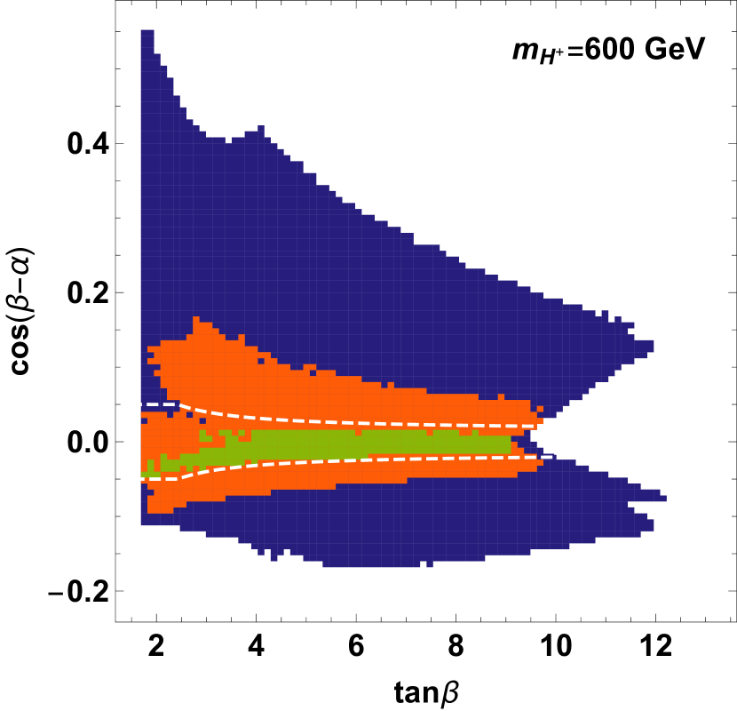
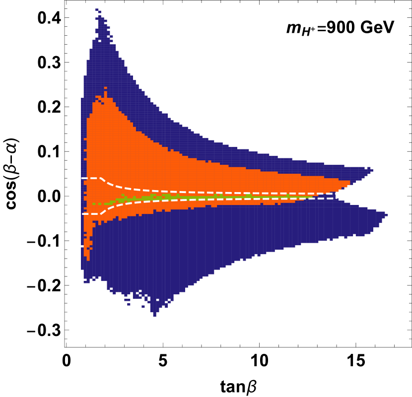
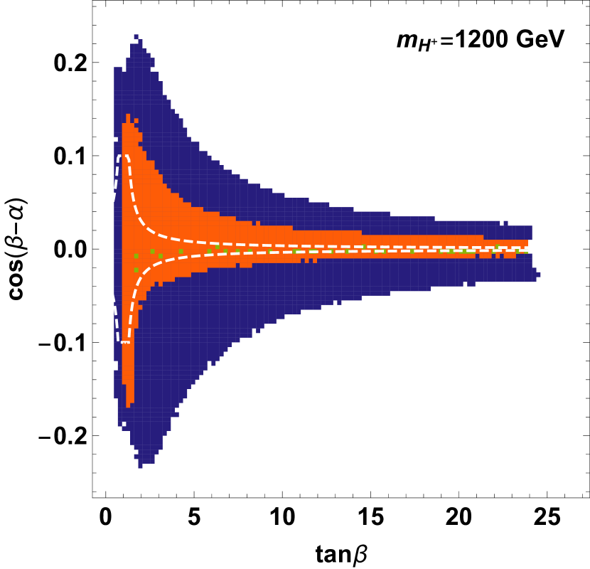
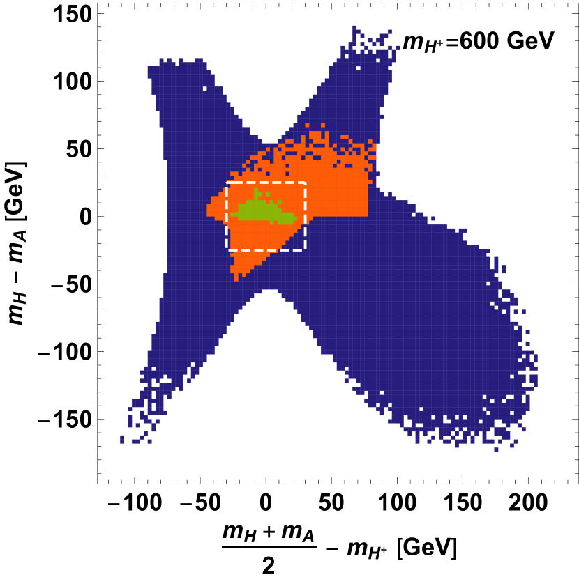
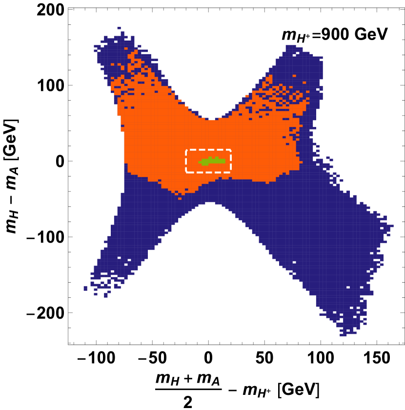
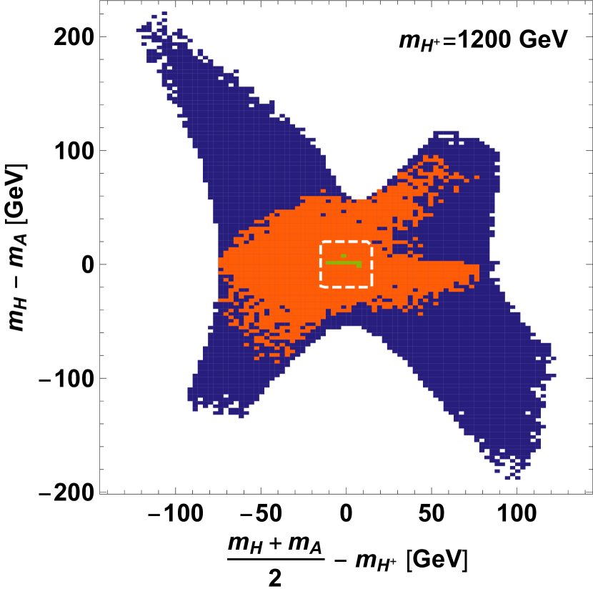
Figure 4: Binned plots of allowed data points. The left, the middle and the right panels correspond to the parameter slices of (i), (ii) and (iii), respectively. All the colored points satisfy the low energy constraints. The orange and the green points satisfy the perturbative unitarity conditions until the Planck scale. The green points satisfy the vacuum stability condition. The regions surrounded by the white dashed lines are used in Fig 5.

A similar condition as the vacuum stability is the bounded-from-below condition, which is given by

$$\lambda_{1}>0~{}\&~{}\lambda_{2}>0~{}\&~{}\left(\frac{\lambda_{1}\lambda_{2}-\bar{\lambda}^{2}}{\lambda_{1}+\lambda_{2}-2\bar{\lambda}}>0~{}{\rm or}~{}\frac{\lambda_{1}-\bar{\lambda}}{\lambda_{2}-\bar{\lambda}}<0\right).$$ (58)

Here, we regard those couplings as the $\overline{\rm MS}$ couplings at $\mu=m_{t}$ and impose it only at low energy. Notice that the condition is obtained from the discussion of Section III and is equivalent to that in Deshpande and Ma (1978). We expect that the combination of the HE perturbative unitarity and the bounded-from-below condition should give a similar result, which we will see below.

In Fig. 5, we pick up the parameter space defined by the region surrounded by the white dashed lines in Fig. 4 and prepare additional five million points satisfying all the low energy constraints for each region. The scattering region is taken so that it can cover all the green points. The distribution of the new data points is uniform in the space of $\tan\beta$, $\cos(\beta-\alpha)/|\cos(\beta-\alpha)|_{\max}$, $m_{H}-m_{A}$ and $(m_{H}+m_{A})/2-m_{H^{+}}$. Here, $|\cos(\beta-\alpha)|_{\max}$ is the maximum value of $\cos(\beta-\alpha)$ depending on $\tan\beta$, which is shown in Fig. 4. The red points satisfy the bounded-from-below condition and the HE perturbative unitarity. The lighter and the darker green points correspond to the green points in Fig. 4 and are plotted over the red points. Thus, in the red region appearing in the figure, the potential is stable at low energy, but always becomes unstable at high energy. The darker green points satisfy both the vacuum stability and the bounded-from-below conditions. Thus, in the lighter green region, the potential always becomes unstable at low energy, but the instability is cured at high energy. Notice that the vacuum decay rates can be affected by the IR cut-off for the $R$ integral in the lighter green region.

As we can see from the figure, the bounded-from-below condition has a similar effect as the vacuum stability condition, but the allowed regions do not overlap completely. In particular, a large part of the region with $m_{H}<m_{A}$ is excluded by the vacuum stability, where $\lambda_{2}$ tends to become negative during the RG evolution. In addition, a negative $\cos(\beta-\alpha)$ is more favored by the vacuum stability.

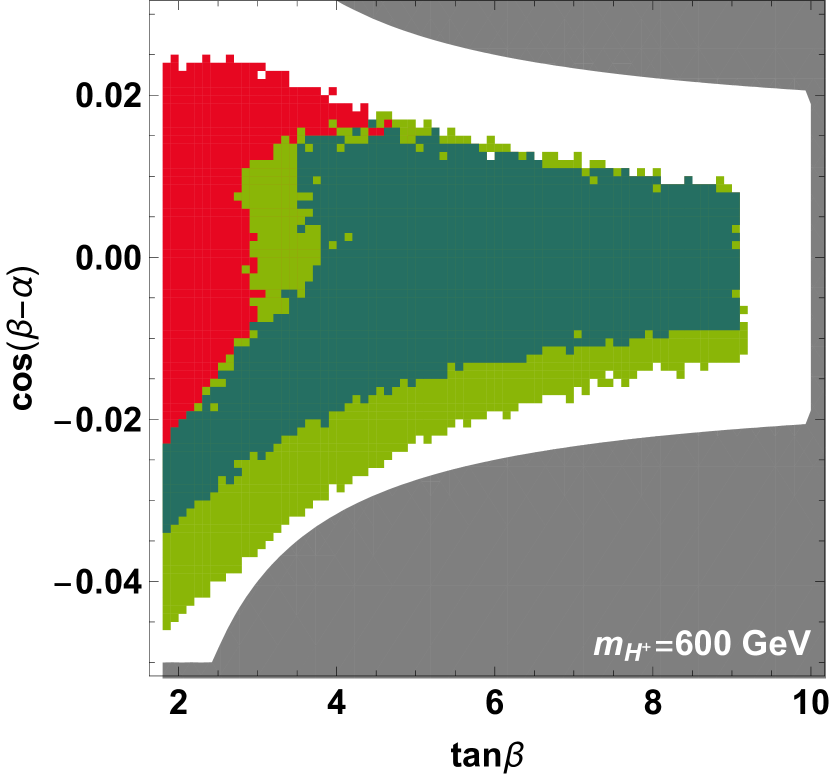
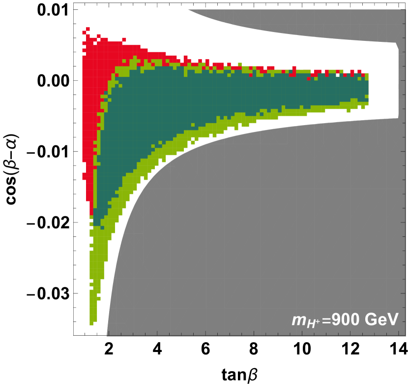
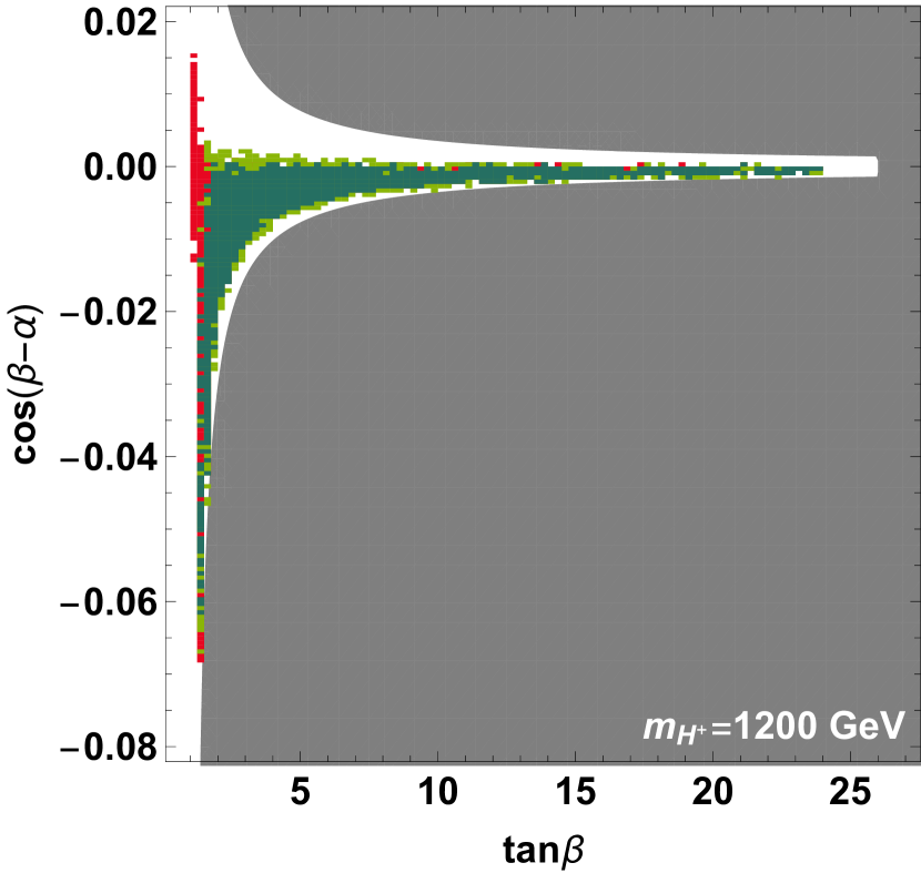
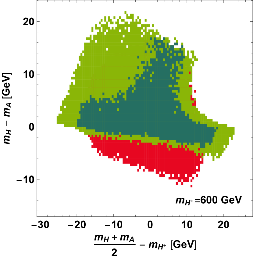
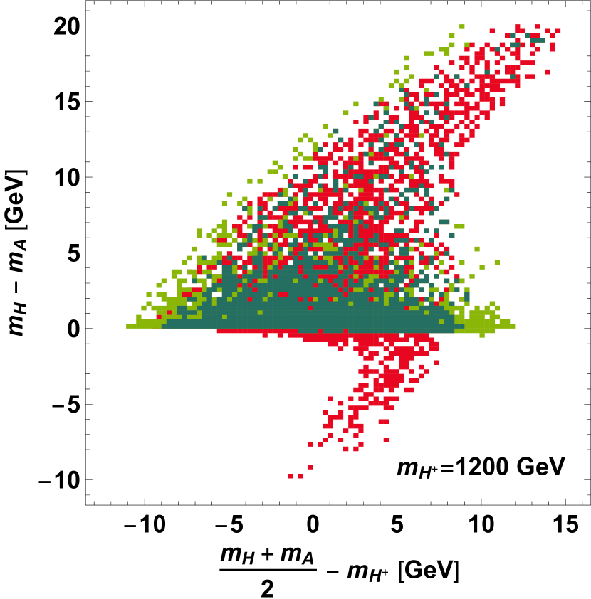
Figure 5: The detail views of the parameter regions inside the white dashed lines in Fig. 4. The masked region is shaded with gray. All the points satisfy the low energy constraints and remain perturbative until the Planck scale. The red points satisfy the bounded-from-below constraint. The lighter green points satisfy the vacuum stability constraint. The darker green points satisfy both of them.

Let us discuss the implication on the Higgs couplings. At the tree level, the SM-value normalized couplings of the $125~{}{\rm GeV}$ Higgs boson are given by

$$g_{hUU} =\sin(\beta-\alpha)+\cot\beta\cos(\beta-\alpha),$$ (59)

$$g_{hDD} =\sin(\beta-\alpha)-\tan\beta\cos(\beta-\alpha),$$ (60)

$$g_{hLL} =\sin(\beta-\alpha)-\tan\beta\cos(\beta-\alpha),$$ (61)

$$g_{hVV} =\sin(\beta-\alpha),$$ (62)

where $U,D,L$, and $V$ represent the up-type quarks, the down-type quarks, the leptons, and the gauge bosons, respectively. Since $|\cos(\beta-\alpha)|\lesssim 0.06$ for all the slices, we have $0.9982\lesssim g_{hVV}\leq 1$, which is not possible to be distinguished from unity even with HL-LHC plus $1~{}{\rm TeV}$ ILC Fujii et al. (2019). It also means that the model cannot be valid up to the Planck scale if we observe larger deviations of $g_{hVV}$ couplings. On the other hand, the other couplings can deviate by more than $1\%$ because of the second term of the above equations.

In Fig. 6, we cast the data points in Fig. 5 into the $g_{hUU}$ vs $g_{hDD}=g_{hLL}$ plane. The colors are the same as in Fig. 5. As we can see, $g_{hUU}$ can be reduced by about $2\%-5\%$ for each slice, but cannot be enhanced so much. On the other hand, $g_{hDD}$ and $g_{hLL}$ can deviate by about $5\%-12\%$ for each slice, and tend to be enhanced.

The current constraints on these couplings are given by Aad et al. (2019)

$$g_{hZZ} =1.10\pm 0.08,$$ (63)

$$g_{hWW} =1.05\pm 0.08,$$ (64)

$$g_{hbb} =1.06^{+0.19}_{-0.18},$$ (65)

$$g_{htt} =1.02^{+0.11}_{-0.10},$$ (66)

$$g_{h\tau\tau} =1.07\pm 0.15,$$ (67)

with the assumption that there is no new particles in loops and decays. Thus, they have already started to touch the parameter space. Future measurements of the Higgs couplings by, for example, the combination of HL-LHC and ILC will reach the precision of a few percent level Fujii et al. (2019) and will possibly find deviations from the SM values.

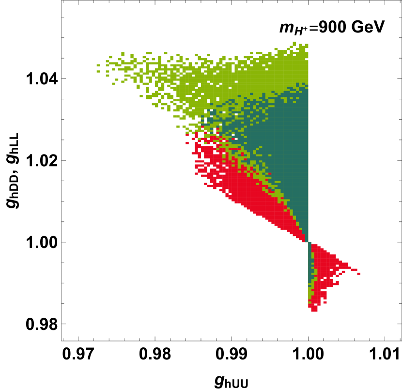
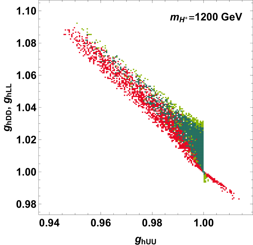
Figure 6: The SM-normalized couplings of the $125~{}{\rm GeV}$ Higgs boson. The colors are the same as in Fig. 5.

Let us discuss the dependence on the IR cut-off and the UV cut-off, which are introduced in Eqs. (32) and (33). Since the beta functions for $\lambda_{1}$ and $\lambda_{2}$ become generically positive at high energy, a factor change of the UV cut-off rarely affects the vacuum decay rate, which we have checked numerically as well. As for the IR cut-off, we have checked that Figs. 5 and 6 are not affected even if we use $1~{}{\rm TeV}$ for the IR cut-off, instead of $10~{}{\rm TeV}$.

Finally, we comment on the effect of $\mathcal{A}$, which we have calculated precisely. Although the vacuum decay rates are enhanced compared with the tree level ones around $\gamma\sim H_{0}^{4}$, we find that the effect is not large enough to change Fig. 6. It is because of the strong dependence of the vacuum decay rates on the Higgs quartic couplings. However, if we find the additional Higgs bosons in future, the vacuum decay rate can be determined precisely from the measurements of the mass differences and the couplings of the Higgs bosons, which will give an important implication on the scenario.

VI Summary

In this paper, we analyzed the high scale validity of the DFSZ axion model, namely the HE perturbative unitarity and the vacuum stability. The model has been widely studied since it can explain the strong CP problem and dark matter elegantly. Once we admit a mechanism that forces classical scale invariance at the Planck scale, the Higgs mass terms of the appropriate size can be generated through the technically natural parameters and may be valid up to the Planck scale. In addition, the model can be extended without affecting the Higgs sector to explain the neutrino masses, the baryon asymmetry of the Universe and inflation. Thus, the high scale behavior of the Higgs sector is worth discussing.

We utilized the state-of-the-art method to calculate the vacuum decay rate precisely. We extended the results of Andreassen et al. (2018); Chigusa et al. (2017, 2018) to accommodate bounces that are composed of more than one fields. Then, we showed that $\mathcal{A}$ can enhance the vacuum decay rates at most by $10^{10}$, which can become comparable with the uncertainties from those of the top mass and the strong coupling constant.

We performed the parameter scan and found the parameter space that satisfies the constraints from flavor observables, LE/HE perturbative unitarity, oblique parameters, collider searches, and vacuum stability. Due to the complementarity of the HE perturbative unitarity and the vacuum stability, the allowed parameter space becomes very small. We observe that it still accommodates at most $12\%$ enhancement of the $hDD$ and $hLL$ couplings, and at most $5\%$ suppression of the $hUU$ couplings. These are around the current experimental constraints and will be searched at future experiments such as HL-LHC and ILC. On the other hand, the deviation of the $hVV$ couplings are found to be smaller than $0.2\%$ and the scenario may be excluded if we observe large deviations of these couplings.

Appendix A Flavor

In this appendix, we follow Enomoto and Watanabe (2016) and obtain the flavor constraints with the current experimental values.

A.1 CKM Matrix Elements

We first determine the CKM matrix elements by using observables that are insensitive to the additional Higgs bosons.

We use the Wolfenstein parametrization defined as

$$V_{\rm CKM}=\begin{pmatrix}1-\frac{\lambda_{\rm CKM}^{2}}{2}&\lambda_{\rm CKM}&A_{\rm CKM}\lambda_{\rm CKM}^{3}(\rho_{\rm CKM}-i\eta_{\rm CKM})\\ -\lambda_{\rm CKM}&1-\frac{\lambda_{\rm CKM}^{2}}{2}&A_{\rm CKM}\lambda_{\rm CKM}^{2}\\ A_{\rm CKM}\lambda_{\rm CKM}^{3}(1-\rho_{\rm CKM}-i\eta_{\rm CKM})&-A_{\rm CKM}\lambda_{\rm CKM}^{2}&1\end{pmatrix},$$ (68)

where we neglect $\mathcal{O}(\lambda_{\rm CKM}^{4})$. We determine $\lambda_{\rm CKM}$ by using the super allowed nuclear beta decays, $|V_{ud}|=0.97420\pm 0.00021$ Hardy and Towner (2016), and the $K\to e\nu$ decay, ${\rm BR}(K\to e\nu)=(1.582\pm 0.007)\times 10^{-5}$ Tanabashi et al. (2018). Combining these two, we obtain

$$\lambda_{\rm CKM} =0.2244\pm 0.0005.$$ (69)

Here, we have used experimental values for the $K$ meson in Table 2.

Next, we determine $A_{\rm CKM}$ from $|V_{cb}|$ assuming that the corrections from the charged Higgs boson are small, which is justified for $m_{H^{+}}>150~{}{\rm GeV}$ and $\tan\beta<100$ Enomoto and Watanabe (2016). We use $|V_{cb}|=(39.25\pm 0.56)\times 10^{-3}$ Amhis et al. (2019) and get

$$A_{\rm CKM}=0.779\pm 0.012.$$ (70)

Finally, we determine $\rho_{\rm CKM}$ and $\eta_{\rm CKM}$ from the unitary triangle. From $\phi_{1}=(22.2\pm 0.7)^{\circ}$, $\phi_{2}=(84.9\pm 5)^{\circ}$, and $\phi_{3}=(71.1\pm 5)^{\circ}$ Amhis et al. (2019), we get

$$\bar{\rho}_{\rm CKM} =0.117\pm 0.020,$$ (71)

$$\bar{\eta}_{\rm CKM} =0.361\pm 0.012,$$ (72)

where

$$\rho_{\rm CKM}+i\eta_{\rm CKM}=\frac{\bar{\rho}_{\rm CKM}+i\bar{\eta}_{\rm CKM}}{1-A_{\rm CKM}^{2}\lambda_{\rm CKM}^{4}(\bar{\rho}_{\rm CKM}+i\bar{\eta}_{\rm CKM})}\sqrt{\frac{1-A_{\rm CKM}^{2}\lambda_{\rm CKM}^{4}}{1-\lambda_{\rm CKM}^{2}}}.$$ (73)

Mesons
Input	Value
$m_{K^{\pm}}$	$493.677~{}{\rm MeV}$ Tanabashi et al. (2018)
$m_{B^{\pm}}$	$5.27933~{}{\rm GeV}$ Tanabashi et al. (2018)
$m_{B_{s}}$	$5.36688~{}{\rm GeV}$ Tanabashi et al. (2018)
$\tau_{K^{\pm}}$	$12.38\pm 0.02~{}{\rm ns}$ Tanabashi et al. (2018)
$\tau_{B^{\pm}}$	$1.638\pm 0.004~{}{\rm ps}$ Tanabashi et al. (2018)
$\tau_{B_{s}}^{H}$	$1.619\pm 0.009~{}{\rm ps}$ Tanabashi et al. (2018)
$\tau_{B_{s}}^{L}$	$1.414\pm 0.006~{}{\rm ps}$ Tanabashi et al. (2018)

Theoretical Inputs
Input	Value
${\rm BR}(b\to s\gamma)^{\rm SM}_{E_{\gamma}>1.6{\rm GeV}}$	$(3.36\pm 0.23)\times 10^{-4}$ Misiak et al. (2015); Czakon et al. (2015)
$f_{K}$	$155.7\pm 0.3~{}{\rm MeV}$ Aoki et al. (2019)
$f_{B}$	$190.0\pm 1.3~{}{\rm MeV}$ Aoki et al. (2019)
$f_{B_{s}}$	$230.3\pm 1.3~{}{\rm MeV}$ Aoki et al. (2019)
$f_{B_{s}}^{2}B^{(s)}_{2}(m_{b})$	$0.0421\pm 0.0028~{}{\rm GeV}^{2}$ Bazavov et al. (2016)
$f_{B_{s}}^{2}B^{(s)}_{3}(m_{b})$	$0.0576\pm 0.0078~{}{\rm GeV}^{2}$ Bazavov et al. (2016)
$\hat{B}_{B_{s}}$	$1.35\pm 0.06$ Aoki et al. (2019)

Table 2: Experimental and theoretical parameters for mesons. The uncertainties are used for the evaluation of theoretical uncertainties in the flavor analysis.

EW Parameters
Input	Value
$m_{h}$	$125.1\pm 0.14~{}{\rm GeV}$ Tanabashi et al. (2018)
$m_{W}$	$80.379~{}{\rm GeV}$ Tanabashi et al. (2018)
$m_{Z}$	$91.1876~{}{\rm GeV}$ Tanabashi et al. (2018)
$\alpha_{s}(m_{Z})$	$0.1181$ Tanabashi et al. (2018)
$G_{F}$	$1.1663787\times 10^{-5}~{}{\rm GeV}^{-2}$ Tanabashi et al. (2018)
$\sin^{2}\theta_{W}(m_{Z})$	$0.23122$ Tanabashi et al. (2018)

Fermion Masses
Input	Value
$M_{t}$	$173.1\pm 0.9~{}{\rm GeV}$ Tanabashi et al. (2018)
$m_{b}(m_{b})$	$4.198\pm 0.012~{}{\rm GeV}$ Aoki et al. (2019)
$m_{s}(2~{}{\rm GeV})$	$93.44\pm 0.68~{}{\rm MeV}$ Aoki et al. (2019)
$m_{u}(2~{}{\rm GeV})$	$2.50\pm 0.17~{}{\rm MeV}$ Aoki et al. (2019)
$m_{\mu}$	$105.6583745~{}{\rm MeV}$ Tanabashi et al. (2018)
$m_{\tau}$	$1.77686~{}{\rm GeV}$ Tanabashi et al. (2018)

Table 3: Fundamental parameters of the SM. The uncertainties are used for the evaluation of theoretical uncertainties in the flavor analysis. The top mass is the on-shell mass and the other quark masses are the $\overline{\rm MS}$ masses with the renormalization scale shown in the parentheses.

Experimental Results
Observable	Value
${\rm BR}(b\to s\gamma)_{E_{\gamma}>1.6{\rm GeV}}$	$(3.32\pm 0.15)\times 10^{-4}$ Amhis et al. (2019)
${\rm BR}(B\to\tau\nu)$	$(1.06\pm 0.19)\times 10^{-4}$ Amhis et al. (2019)
${\rm BR}(B_{s}\to\mu\mu)$	$(3.1\pm 0.6)\times 10^{-9}$ Amhis et al. (2019)
$\Delta M_{B_{s}}$	$17.757\pm 0.021~{}{\rm ps}^{-1}$ Amhis et al. (2019)

Table 4: Experimental results for flavor observables.

A.2 Flavor Constraints

For the theoretical evaluation of the flavor observables, we use the formulas given in Enomoto and Watanabe (2016). In the calculation, we utilize RunDec Chetyrkin et al. (2000); Herren and Steinhauser (2018) to get the running masses of quarks.

Let us clarify the statistical method that we adopt. For observable $X$ that depends on known parameters $\{x_{i}\pm\delta x_{i}\}$ and model parameters $\{y_{i}\}$, we define

$$\chi^{2}(\{y_{i}\})=\frac{(X(\{y_{i}\})-X_{\rm exp})^{2}}{\delta X_{\rm th}^{2}(\{y_{i}\})+\delta X_{\rm exp}^{2}},$$ (74)

where $X_{\rm exp}\pm\delta X_{\rm exp}$ is the experimental result, $X(\{y_{i}\})$ is the theoretical result for inputs $\{x_{i}\}$ and $\{y_{i}\}$, and

$$\delta X_{\rm th}^{2}(\{y_{i}\})=\sum_{k}\left[X(\{y_{i}\})|_{x_{k}\to x_{k}+\delta x_{k}/2}-X(\{y_{i}\})|_{x_{k}\to x_{k}-\delta x_{k}/2}\right]^{2}.$$ (75)

Then, we use the offset corrected $\chi^{2}$ defined as

$$\Delta\chi^{2}(\{y_{i}\})=\chi^{2}(\{y_{i}\})-\min_{\{\tilde{y}_{i}\}}\chi^{2}(\{\tilde{y}_{i}\}),$$ (76)

and the $95\%$ CL exclusion limit is given by $\Delta\chi^{2}(\{y_{i}\})\lesssim 3.84$. Here, the minimum value is searched over the parameter space of Fig. 3 and the SM limit. The known parameters $\{x_{i}\pm\delta x_{i}\}$ are summarized in Tables 2 and 3, where we ignore uncertainties of $\mathcal{O}(0.1\%)$.

The result is shown in Fig. 3.

Appendix B Proof of Straight Bounce

In this appendix, we show that $\Omega$ and $\Theta$ of the relevant solution do not depend on $r$. In terms of $\phi$, $\Omega$ and $\Theta$, the Euclidean action is expressed as

$$S_{E}[\phi,\Omega,\Theta] =\mathcal{K}[\phi,\Omega,\Theta]+\mathcal{V}[\phi,\Omega,\Theta],$$ (77)

$$\mathcal{K}[\phi,\Omega,\Theta] =2\pi^{2}\int drr^{3}\left[\frac{1}{2}\phi^{\prime 2}+\frac{1}{2}\phi^{2}\left(\Omega^{\prime 2}+\Theta^{\prime 2}\sin^{2}\Omega\right)\right],$$ (78)

$$\mathcal{V}[\phi,\Omega,\Theta] =2\pi^{2}\int drr^{3}\frac{\lambda_{\phi}}{4}\phi^{4},$$ (79)

where $\Omega^{\prime}$, $\Theta^{\prime}$ and $\phi^{\prime}$ are derivatives with respect to $r$. As introduced in Coleman et al. (1978), we can obtain the bounce by minimizing $\mathcal{K}[\tilde{\phi},\tilde{\Omega},\tilde{\Theta}]$ with the constraint given by

$$\mathcal{V}[\tilde{\phi},\tilde{\Omega},\tilde{\Theta}] =({\rm const.})<0.$$ (80)

After the minimization, the bounce solution is obtained as

$$\phi(r)=\tilde{\phi}(\sigma r),~{}\Omega(r)=\tilde{\Omega}(\sigma r),~{}\Theta(r)=\tilde{\Theta}(\sigma r),$$ (81)

where

$$\sigma=\sqrt{-\frac{2\mathcal{V}[\tilde{\phi},\tilde{\Omega},\tilde{\Theta}]}{\mathcal{K}[\tilde{\phi},\tilde{\Omega},\tilde{\Theta}]}}.$$ (82)

Its Euclidean action is given by

$$S_{E}=\frac{\mathcal{K}[\tilde{\phi},\tilde{\Omega},\tilde{\Theta}]}{2\sigma^{2}}.$$ (83)

Let us assume that there exists a minimum, $\mathcal{K}[\tilde{\phi}_{A},\tilde{\Omega}_{A},\tilde{\Theta}_{A}]$, where $\tilde{\Omega}_{A}$ or $\tilde{\Theta}_{A}$ is not constant. Since $\lambda_{\phi}(\Omega,\Theta)$ is a continuous function, there exist constant $\Omega_{B}$ and $\Theta_{B}$ satisfying

$$\mathcal{V}[\tilde{\phi}_{A},\tilde{\Omega}_{A},\tilde{\Theta}_{A}]=\mathcal{V}[\tilde{\phi}_{A},\Omega_{B},\Theta_{B}].$$ (84)

Then, we have

$$\mathcal{K}[\tilde{\phi}_{A},\tilde{\Omega}_{A},\tilde{\Theta}_{A}]-\mathcal{K}[\tilde{\phi}_{A},\Omega_{B},\Theta_{B}]=2\pi^{2}\int drr^{3}\frac{1}{2}\tilde{\phi}_{A}^{2}\left(\tilde{\Omega}^{\prime 2}_{A}+\tilde{\Theta}^{\prime 2}_{A}\sin^{2}\tilde{\Omega}_{A}\right)\geq 0.$$ (85)

The equality holds only when $\tilde{\Omega}^{\prime}(r)=\tilde{\Theta}^{\prime}(r)=0$ for any $r$. Notice that when $\sin\tilde{\Omega}_{A}=0$, the field space is not parameterized by $\tilde{\Theta}_{A}$. Then, from Eq. (83), there exists a bounce with smaller action if $\tilde{\Omega}$ or $\tilde{\Theta}$ is not constant. Thus, the bounce with minimum action can only be realized with constant $\Omega$ and $\Theta$.

Appendix C One-loop Corrections to a Vacuum Decay Rate

From Chigusa et al. (2018), the differential vacuum decay rate is expressed as

$$\frac{d\gamma}{dR} =\left.\frac{1}{R^{5}}\mathcal{A}^{\prime(h)}\mathcal{A}^{(\sigma)}\mathcal{A}^{(\psi)}\mathcal{A}^{(A_{\mu},\varphi)}e^{-\mathcal{B}}\right|_{\mu\sim R^{-1}},$$ (86)

where

$$\ln\mathcal{A}^{\prime(h)} =\left.\left[\ln\mathcal{A}^{\prime(h)}\right]_{\overline{\rm MS}}\right|_{\lambda\to\lambda_{\phi}},$$ (87)

$$\ln\mathcal{A}^{(\sigma)} =\sum_{i}\left.n_{i}^{(\sigma)}\left[\ln\mathcal{A}^{(\sigma)}\right]_{\overline{\rm MS}}\right|_{\kappa\to\kappa_{i},~{}\lambda\to\lambda_{\phi}},$$ (88)

$$\ln\mathcal{A}^{(\psi)} =\sum_{i}\left.n_{i}^{(\psi)}\left[\ln\mathcal{A}^{(\psi)}\right]_{\overline{\rm MS}}\right|_{y\to y_{i},~{}\lambda\to\lambda_{\phi}},$$ (89)

$$\ln\mathcal{A}^{(A_{\mu},\varphi)} =\ln\mathcal{V}_{G}+\sum_{i}\left.n_{i}^{(A_{\mu},\varphi)}\left[\ln\mathcal{A}^{\prime(A_{\mu},\varphi)}\right]_{\overline{\rm MS}}\right|_{g^{2}\to\tilde{g}_{i}^{2},~{}\lambda\to\lambda_{\phi}}.$$ (90)

Here, $[\ln\mathcal{A}^{(X)}]_{\overline{\rm MS}}$’s are defined in Chigusa et al. (2018). The degrees of freedom, $n_{i}^{(X)}$, and the couplings, $\kappa_{i}$, $y_{i}$ and $g_{i}^{2}$, are summarized below for each case. For case (c), the symmetry breaking pattern depends on the sign of $\lambda_{4}$. Thus, we divide it into two cases; (c.1): $\lambda_{4}<0$ and (c.2): $\lambda_{4}>0$.

case (a)

$\lambda_{\phi}=\frac{1}{2}\lambda_{1}$

The scalar contributions:

$$n_{1}^{(\sigma)}=2, ~{}\kappa_{1}=\frac{\lambda_{3}}{2},$$ (91)

$$n_{2}^{(\sigma)}=2, ~{}\kappa_{2}=\frac{\lambda_{3}+\lambda_{4}}{2}.$$ (92)

The fermion contributions:

$$n_{1}^{(\psi)}=3, ~{}y_{1}=y_{b},$$ (93)

$$n_{2}^{(\psi)}=1, ~{}y_{2}=y_{\tau}.$$ (94)

The gauge boson contributions:

$$n_{1}^{(A_{\mu},\varphi)}=2, ~{}\tilde{g}_{1}^{2}=\frac{g_{2}^{2}}{4},$$ (95)

$$n_{2}^{(A_{\mu},\varphi)}=1, ~{}\tilde{g}_{2}^{2}=\frac{g_{Y}^{2}+g_{2}^{2}}{4}.$$ (96)

case (b)

$\lambda_{\phi}=\frac{1}{2}\lambda_{2}$

The scalar contributions:

$$n_{1}^{(\sigma)}=2, ~{}\kappa_{1}=\frac{\lambda_{3}}{2},$$ (97)

$$n_{2}^{(\sigma)}=2, ~{}\kappa_{2}=\frac{\lambda_{3}+\lambda_{4}}{2}.$$ (98)

The fermion contributions:

$$n_{1}^{(\psi)}=3, ~{}y_{1}=y_{t}.$$ (99)

The gauge boson contributions:

$$n_{1}^{(A_{\mu},\varphi)}=2, ~{}\tilde{g}_{1}^{2}=\frac{g_{2}^{2}}{4},$$ (100)

$$n_{2}^{(A_{\mu},\varphi)}=1, ~{}\tilde{g}_{2}^{2}=\frac{g_{Y}^{2}+g_{2}^{2}}{4}.$$ (101)

case (c.1)

$\lambda_{\phi}=\frac{1}{2}\frac{\lambda_{1}\lambda_{2}-(\lambda_{3}+\lambda_{4})^{2}}{\lambda_{1}+\lambda_{2}-2(\lambda_{3}+\lambda_{4})}$

The scalar contributions:

$$n_{1}^{(\sigma)}=2, ~{}\kappa_{1}=\lambda_{\phi}+\frac{|\lambda_{4}|}{2},$$ (102)

$$n_{2}^{(\sigma)}=1, ~{}\kappa_{2}=\lambda_{\phi}+\frac{(\lambda_{3}+\lambda_{4}-\lambda_{1})(\lambda_{3}+\lambda_{4}-\lambda_{2})}{\lambda_{1}+\lambda_{2}-2(\lambda_{3}+\lambda_{4})},$$ (103)

$$n_{3}^{(\sigma)}=1, ~{}\kappa_{3}=\lambda_{\phi}.$$ (104)

The fermion contributions:

$$n_{1}^{(\psi)}=3, ~{}y_{1}=y_{t}\sqrt{\frac{\lambda_{1}-\lambda_{3}-\lambda_{4}}{\lambda_{1}+\lambda_{2}-2(\lambda_{3}+\lambda_{4})}},$$ (105)

$$n_{2}^{(\psi)}=3, ~{}y_{2}=y_{b}\sqrt{\frac{\lambda_{2}-\lambda_{3}-\lambda_{4}}{\lambda_{1}+\lambda_{2}-2(\lambda_{3}+\lambda_{4})}},$$ (106)

$$n_{3}^{(\psi)}=1, ~{}y_{3}=y_{\tau}\sqrt{\frac{\lambda_{2}-\lambda_{3}-\lambda_{4}}{\lambda_{1}+\lambda_{2}-2(\lambda_{3}+\lambda_{4})}}.$$ (107)

The gauge boson contributions:

$$n_{1}^{(A_{\mu},\varphi)}=2, ~{}\tilde{g}_{1}^{2}=\frac{g_{2}^{2}}{4},$$ (108)

$$n_{2}^{(A_{\mu},\varphi)}=1, ~{}\tilde{g}_{2}^{2}=\frac{g_{Y}^{2}+g_{2}^{2}}{4}.$$ (109)

case (c.2)

$\lambda_{\phi}=\frac{1}{2}\frac{\lambda_{1}\lambda_{2}-\lambda_{3}^{2}}{\lambda_{1}+\lambda_{2}-2\lambda_{3}}$

The scalar contributions:

$$n_{1}^{(\sigma)}=2, ~{}\kappa_{1}=\lambda_{\phi}+\frac{|\lambda_{4}|}{2},$$ (110)

$$n_{2}^{(\sigma)}=1, ~{}\kappa_{2}=\lambda_{\phi}+\frac{(\lambda_{3}-\lambda_{1})(\lambda_{3}-\lambda_{2})}{\lambda_{1}+\lambda_{2}-2\lambda_{3}}.$$ (111)

The fermion contributions:

$$n_{1}^{(\psi)}=3, ~{}y_{1}=\sqrt{y_{t}^{2}\frac{\lambda_{1}-\lambda_{3}}{\lambda_{1}+\lambda_{2}-2\lambda_{3}}+y_{b}^{2}\frac{\lambda_{2}-\lambda_{3}}{\lambda_{1}+\lambda_{2}-2\lambda_{3}}},$$ (112)

$$n_{2}^{(\psi)}=1, ~{}y_{2}=y_{\tau}\sqrt{\frac{\lambda_{2}-\lambda_{3}}{\lambda_{1}+\lambda_{2}-2\lambda_{3}}}.$$ (113)

The gauge boson contributions:

$$n_{1}^{(A_{\mu},\varphi)}=2, ~{}\tilde{g}_{1}^{2}=\frac{g_{2}^{2}}{4},$$ (114)

$$n_{2}^{(A_{\mu},\varphi)}=1, ~{}\tilde{g}_{2}^{2}=\frac{g_{Y}^{2}+g_{2}^{2}+\sqrt{(g_{Y}^{2}-g_{2}^{2})^{2}+4g_{Y}^{2}g_{2}^{2}\left(\frac{\lambda_{1}-\lambda_{2}}{\lambda_{1}+\lambda_{2}-2\lambda_{3}}\right)^{2}}}{8},$$ (115)

$$n_{3}^{(A_{\mu},\varphi)}=1, ~{}\tilde{g}_{3}^{2}=\frac{g_{Y}^{2}+g_{2}^{2}-\sqrt{(g_{Y}^{2}-g_{2}^{2})^{2}+4g_{Y}^{2}g_{2}^{2}\left(\frac{\lambda_{1}-\lambda_{2}}{\lambda_{1}+\lambda_{2}-2\lambda_{3}}\right)^{2}}}{8}.$$ (116)

Here, $g_{Y}$ and $g_{2}$ are the gauge couplings for $U(1)_{Y}$ and $SU(2)_{L}$, respectively. The group volume is $\mathcal{V}_{G}=2\pi^{2}$ for cases (a), (b) and (c.1), and $\mathcal{V}_{G}=4\pi^{3}$ for case (c.2).

Notice that we can determine whether a solution, $\phi$, is a minimum or not from the sign of $\kappa_{i}-\lambda_{\phi}$. Let $\chi_{i}$ be a scalar orthogonal to $\phi$. Then, its potential can be written as

$$V(\chi_{i})=\frac{\lambda_{\phi}}{4}(\phi^{2}+\chi_{i}^{2})^{2}+\frac{\delta}{2}\phi^{2}\chi_{i}^{2}+\dots,$$ (117)

where $\delta$ breaks the rotational symmetry of $(\phi,\chi_{i})$. Since $\kappa_{i}$ can be read off from the mass term for $\chi_{i}$, we get

$$\kappa_{i}=\lambda_{\phi}+\delta.$$ (118)

Thus, for $\phi$ to be a minimum of the action, we need $\kappa_{i}-\lambda_{\phi}>0$ for all $i$.

For case (c.1), we have $\kappa_{3}=\lambda_{\phi}$ and thus there appears a zero mode, which is due to the spontaneous breaking of the PQ symmetry. Its treatment is discussed in Appendix E of Chigusa et al. (2018) and we replace

$$\left.n_{3}^{(\sigma)}\left[\ln\mathcal{A}^{(\sigma)}\right]_{\overline{\rm MS}}\right|_{\kappa\to\kappa_{3},\lambda\to\lambda_{\phi}}\to\mathcal{V}_{\sigma}\left.n_{3}^{(\sigma)}\left[\ln\mathcal{A}^{\prime(A_{\mu},\varphi)}\right]_{\overline{\rm MS}}\right|_{g^{2}\to 0,~{}\lambda\to\lambda_{\phi}},$$ (119)

with $\mathcal{V}_{\sigma}=2\pi$.

Appendix D Matching Conditions

This appendix is devoted to the explanation of the one-loop matching conditions for the dimensionless coupling constants. The matching scale is taken to be $\mu_{t}=m_{t}$. For a detailed discussion of the renormalization scheme, see Denner (1993); Altenkamp et al. (2017). We assume that $\tan\beta$ and $\cos(\beta-\alpha)$ are renormalized with the ${\rm\overline{MS}}$ scheme. In the calculation of one-loop threshold corrections, we utilize the public codes of SARAH Staub et al. (2012); Staub (2015), FeynArts Hahn (2001), FeynCalc Mertig et al. (1991); Shtabovenko et al. (2016).

D.1 Gauge Couplings

We first evaluate the electric charge at $\mu_{t}$ as

$$\frac{[e^{\rm SM(5)}(\mu_{t})]^{2}}{4\pi}=\frac{\alpha^{\rm SM(5)}(m_{Z})}{1-\frac{b^{\rm SM(5)}_{e}}{2\pi}\alpha^{\rm SM(5)}(m_{Z})\ln\frac{\mu_{t}}{m_{Z}}},$$ (120)

where Tanabashi et al. (2018)

$$[\alpha^{{\rm SM}(5)}(m_{Z})]^{-1} =127.955\pm 0.010,$$ (121)

$$b^{\rm SM(5)}_{e} =\frac{38}{9}.$$ (122)

It is then matched to the THDM electric charge as

$$e(\mu_{t})=\frac{e^{\rm SM(5)}(\mu_{t})}{1-\Delta e},$$ (123)

where

$$\Delta e=-\frac{[e^{\rm SM(5)}(\mu_{t})]^{2}}{16\pi^{2}}\left(-7\ln\frac{m_{W}}{\mu_{t}}+\frac{1}{3}+\frac{16}{9}\ln\frac{m_{t}}{\mu_{t}}+\frac{1}{3}\ln\frac{m_{H^{+}}}{\mu_{t}}\right).$$ (124)

Next, we calculate the ${\rm\overline{MS}}$ masses of the gauge bosons as

$$m_{V}^{2}(\mu_{t})=m_{V}^{2,{\rm OS}}+\bar{\Sigma}^{T}_{V}(m_{V}^{2}),$$ (125)

with $V=W,Z$. Here, $\bar{\Sigma}^{T}_{V}(p^{2})$ is the self energy for the transverse mode with $1/\bar{\varepsilon}$ being subtracted. Here,

$$\frac{1}{\bar{\varepsilon}}=\frac{2}{4-D}-\gamma_{E}+\ln 4\pi,$$ (126)

where $D$ is the spacetime dimension and $\gamma_{E}$ is the Euler number. The superscript, ${\rm OS}$, indicates the on-shell mass.

Using these, the Weinberg angle is calculated as

$$\cos\theta_{W}(\mu_{t}) =\frac{m_{W}(\mu_{t})}{m_{Z}(\mu_{t})}.$$ (127)

Then, the ${\rm\overline{MS}}$ gauge couplings are given by

$$g_{Y}(\mu_{t}) =\frac{e(\mu_{t})}{\cos\theta_{W}(\mu_{t})},$$ (128)

$$g_{2}(\mu_{t}) =\frac{e(\mu_{t})}{\sin\theta_{W}(\mu_{t})}.$$ (129)

Finally, the strong coupling constant is evaluated with RunDec Chetyrkin et al. (2000); Herren and Steinhauser (2018). Notice that there are no one-loop threshold corrections from the additional Higgs bosons.

For the later convenience, let us define

$$v(\mu_{t})=\frac{2\sin\theta_{W}(\mu_{t})}{e(\mu_{t})}m_{W}(\mu_{t}).$$ (130)

D.2 Yukawa Couplings

The ${\rm\overline{MS}}$ tau mass is obtained from

$$m_{\tau}(\mu_{t})=m_{\tau}^{\rm OS}\left[1+\bar{\Sigma}^{S}_{\tau}(m^{2}_{\tau})+\frac{1}{2}\bar{\Sigma}^{L}_{\tau}(m^{2}_{\tau})+\frac{1}{2}\bar{\Sigma}^{R}_{\tau}(m^{2}_{\tau})\right],$$ (131)

where $\bar{\Sigma}^{S}_{\tau}(p^{2})$, $\bar{\Sigma}^{L}_{\tau}(p^{2})$ and $\bar{\Sigma}^{R}_{\tau}(p^{2})$ are the scalar, the left-handed and the right-handed parts of the self energy with $1/\bar{\varepsilon}$ being subtracted.

As for the ${\rm\overline{MS}}$ masses of the top quark and the bottom quark, we include the four-loop QCD corrections by using RunDec Chetyrkin et al. (2000); Herren and Steinhauser (2018). Then, we add the non-QCD one-loop threshold corrections to the output of RunDec as

$$m_{f}(\mu_{t})=m_{f}^{\tt RunDec}(m_{t})\left[1+\bar{\Sigma}^{S}_{f,g_{3}=0}(m_{f}^{2})+\frac{1}{2}\bar{\Sigma}^{L}_{f,g_{3}=0}(m_{f}^{2})+\frac{1}{2}\bar{\Sigma}^{R}_{f,g_{3}=0}(m_{f}^{2})\right],$$ (132)

for $f=t,b$. Here, $m_{f}^{\tt RunDec}(m_{t})$ is the output of RunDec and the subscript $g_{3}=0$ indicates that the strong coupling is switched off in the calculation.

Then, the ${\rm\overline{MS}}$ Yukawa couplings are given by

$$y_{t}(\mu_{t}) =\frac{\sqrt{2}}{\sin\beta(\mu_{t})}\frac{m_{t}(\mu_{t})}{v(\mu_{t})},$$ (133)

$$y_{b}(\mu_{t}) =\frac{\sqrt{2}}{\cos\beta(\mu_{t})}\frac{m_{b}(\mu_{t})}{v(\mu_{t})},$$ (134)

$$y_{\tau}(\mu_{t}) =\frac{\sqrt{2}}{\cos\beta(\mu_{t})}\frac{m_{\tau}(\mu_{t})}{v(\mu_{t})}.$$ (135)

D.3 Higgs Quartic Couplings

To adjust the Higgs VEVs order by order in perturbative expansions, we extend the scalar potential with tadpole terms as

$$V_{\rm THDM}\to V_{\rm THDM}+T_{h}h+T_{H}H,$$ (136)

where $T_{h}$ and $T_{H}$ are zero at the tree level.

The ${\rm\overline{MS}}$ values of these couplings are chosen as

$$T_{X}(\mu_{t})=\bar{\Gamma}_{X}^{(\rm tad)},$$ (137)

with $X=h,H$. Here, $\bar{\Gamma}_{X}^{(\rm tad)}$ is the tadpole contributions to the effective action with $1/\bar{\varepsilon}$ being subtracted.

As for the scalars, the ${\rm\overline{MS}}$ masses are given by

$$m^{2}_{X}(\mu_{t})=m_{X}^{2,{\rm OS}}+\bar{\Sigma}(m_{X}^{2}),$$ (138)

with $X=h,H,A,H^{+}$. Here, $\bar{\Sigma}_{X}(p^{2})$ is the self energy with $1/\bar{\varepsilon}$ being subtracted.

The ${\rm\overline{MS}}$ Higgs quartic couplings are then obtained as

$$\lambda_{1} =\frac{1}{2v^{2}\cos^{2}\beta}\left[m_{h}^{2}+m_{H}^{2}-(1-\cos 2\beta)m_{A}^{2}+(m_{H}^{2}-m_{h}^{2})\cos 2\alpha\right]$$

$$\hskip 12.91663pt+\frac{1}{2v^{3}\cos\beta}\left[(3\cos\alpha-\cos(\alpha-2\beta))T_{H}-(3\sin\alpha-\sin(\alpha-2\beta))T_{h}\right],$$ (139)

$$\lambda_{2} =\frac{1}{2v^{2}\sin^{2}\beta}\left[m_{h}^{2}+m_{H}^{2}-(1+\cos 2\beta)m_{A}^{2}-(m_{H}^{2}-m_{h}^{2})\cos 2\alpha\right]$$

$$\hskip 12.91663pt+\frac{1}{2v^{3}\sin\beta}\left[(3\sin\alpha+\sin(\alpha-2\beta))T_{H}+(3\cos\alpha+\cos(\alpha-2\beta))T_{h}\right],$$ (140)

$$\lambda_{3} =\frac{1}{v^{2}}\left[2m_{H^{+}}^{2}-m_{A}^{2}+(m_{H}^{2}-m_{h}^{2})\frac{\sin 2\alpha}{\sin 2\beta}\right]$$

$$\hskip 12.91663pt+\frac{1}{2v^{3}\sin 2\beta}$$

$$\hskip 21.52771pt\times\left[(3\sin(\alpha+\beta)+\sin(\alpha-3\beta))T_{H}+(3\cos(\alpha+\beta)+\cos(\alpha-3\beta))T_{h}\right],$$ (141)

$$\lambda_{4} =\frac{2}{v^{2}}(m_{A}^{2}-m_{H^{+}}^{2}),$$ (142)

where all the quantities appearing in the right-hand side are the ${\rm\overline{MS}}$ values; we suppressed the renormalization scale, $\mu_{t}$, for visibility.

Appendix E Generation of Data Points

In our analysis, we need to generate data points that consist of $(m_{H},m_{A},\tan\beta,\cos(\beta-\alpha))$ for a fixed $m_{H^{+}}$. We first take a random $\tan\beta$, which is uniformly distributed in the ranges defined in Eqs. (53)-(55). The other variables are generated with the procedure described in this section. The generated data points are then filtered by the perturbative unitarity conditions and are passed to the next analysis. In this appendix, we answer the following questions: (i) what is the appropriate range for $m_{H}$, $m_{A}$ and $\cos(\beta-\alpha)$ that covers all the points allowed by the perturbative unitarity? (ii) how can we effectively generate data points that are allowed by the perturbative unitarity?

A naive answer to question (i) is that $|m_{H^{+}}^{2}-m_{H,A}^{2}|\lesssim 8\pi v^{2}$ and $|\cos(\beta-\alpha)|\leq 1$, where $v\simeq 246~{}{\rm GeV}$. However, they are too weak to be used for the parameter scan. As we can see from Fig. 4, the allowed mass differences are smaller than about $200~{}{\rm GeV}$. However, one realizes that $\sqrt{8\pi}v\simeq 1.2~{}\rm{TeV}$. It also means that $H$ can be as light as $h$ and the mixing angle can become large, which is why we naively expect no constraint on the mixing angle. However, the allowed $|\cos(\beta-\alpha)|$ is smaller than about $0.02$ and becomes much smaller in the large $\tan\beta$ regime. Thus, if we scattered the data points over this naive range, we could get only a very few points that satisfy the low energy constraints. That is why we have question (ii).

E.1 Necessary Conditions for Perturbative Unitarity

Let us first analyze the perturbative unitarity conditions. For arbitrary real numbers $A,B$ and $C$, the inequality,

$$|A\pm\sqrt{B^{2}+C^{2}}|<1,$$ (143)

can be reduced to

$$|C|<\sqrt{(|A|-1)^{2}-B^{2}}~{}\&~{}|A|<1~{}\&~{}|B|<1-|A|.$$ (144)

Applying it to the perturbative unitarity constraints, we get constraints on $\lambda_{1}$ and $\lambda_{2}$ as

$$|\lambda_{1}| <\mathcal{T},$$ (145)

$$|\lambda_{2}| <\mathcal{T},$$ (146)

$$|\lambda_{1}+\lambda_{2}| <\frac{2}{3}\mathcal{T},$$ (147)

$$|\lambda_{1}+\lambda_{2}| <\mathcal{T}+\frac{\lambda_{1}\lambda_{2}}{\mathcal{T}},$$ (148)

$$|\lambda_{1}+\lambda_{2}| <\frac{\mathcal{T}}{3}+\frac{3\lambda_{1}\lambda_{2}}{\mathcal{T}},$$ (149)

which can be reduced to

$$|\lambda_{1}| <\frac{\mathcal{T}}{3},$$ (150)

$$|\lambda_{2}| <\frac{\mathcal{T}}{3}.$$ (151)

Here, $\mathcal{T}=8\pi$. As for $\lambda_{3}$ and $\lambda_{4}$, the constraints have the form of

$$a_{i}\lambda_{3}+b_{i}\lambda_{4} <c_{i},$$ (152)

Here, $a_{i}$’s and $b_{i}$’s are constants and $c_{i}$’s are functions of $\lambda_{1}$ and $\lambda_{2}$.

The range of $\lambda_{3}$ and $\lambda_{4}$ satisfying Eq. (152) can be determined by the simplex method of linear programming. We consider simultaneous equations given by

$$a_{i}\lambda_{3}+b_{i}\lambda_{4}+z_{i} =c_{i},$$ (153)

where $z_{i}$’s are the slack variables. Then, we solve them under the constraint of $z_{k}=z_{l}=0$ for each pair of $(k,l)$. The solutions satisfying $z_{i}\geq 0$ correspond to the corners of the allowed region. We search for such solutions and get

$$|\lambda_{3}| <\frac{\mathcal{T}+\sqrt{\mathcal{T}^{2}-3\mathcal{T}|\lambda_{1}+\lambda_{2}|+9\lambda_{1}\lambda_{2}}}{3}\leq\frac{2}{3}\mathcal{T},$$ (154)

$$|\lambda_{4}| <\frac{2}{3}\mathcal{T},$$ (155)

$$|\lambda_{3}+\lambda_{4}| <\frac{\mathcal{T}+\sqrt{\mathcal{T}^{2}-3\mathcal{T}|\lambda_{1}+\lambda_{2}|+9\lambda_{1}\lambda_{2}}}{3}\leq\frac{2}{3}\mathcal{T},$$ (156)

$$|2\lambda_{3}+\lambda_{4}| <\sqrt{\mathcal{T}^{2}-3\mathcal{T}|\lambda_{1}+\lambda_{2}|+9\lambda_{1}\lambda_{2}}\leq\mathcal{T}.$$ (157)

E.2 Data Generation

Let us go back to the problem of data generation. We define

$$\lambda_{a} =\lambda_{1}\cos^{2}\beta-\lambda_{2}\sin^{2}\beta-(\lambda_{3}+\lambda_{4})\cos 2\beta,$$ (158)

$$\lambda_{b} =\lambda_{1}\cos^{2}\beta+\lambda_{2}\sin^{2}\beta+\frac{\lambda_{4}}{2},$$ (159)

$$\lambda_{c} =\lambda_{1}\cos^{2}\beta-\lambda_{2}\sin^{2}\beta+\lambda_{3}\cos 2\beta.$$ (160)

We will scatter $(\lambda_{a},\lambda_{b},\lambda_{4})$ instead of $(m_{H},m_{A},\cos(\beta-\alpha))$.

We first generate random $(\lambda_{a},\lambda_{b})$. The scattering range is given by

$$|\lambda_{a}| <\frac{\mathcal{T}}{3}\left(1+2|\cos 2\beta|\right),$$ (161)

$$|\lambda_{b}| <\frac{2}{3}\mathcal{T},$$ (162)

which are derived from the inequalities in the previous subsection. We can further constrain the range with

$$m_{H^{+}}^{2}-m_{h}^{2}+\lambda_{b}v^{2} =m_{H}^{2}>0.$$ (163)

Then, we calculate

$$\sin 2(\beta-\alpha) =\frac{\lambda_{a}v^{2}\sin 2\beta}{m_{H^{+}}^{2}-2m_{h}^{2}+\lambda_{b}v^{2}},$$ (164)

$$\lambda_{c} =\frac{2\cos 2\beta}{v^{2}}\left[m_{H^{+}}^{2}+\cos 2(\beta-\alpha)\left(m_{H^{+}}^{2}-2m_{h}^{2}+\lambda_{b}v^{2}\right)\right]$$

$$\hskip 12.91663pt-\lambda_{a}\cos 4\beta,$$ (165)

with the assumption of $\cos 2(\beta-\alpha)<0$, and check

$$|\sin 2(\beta-\alpha)| <1,$$ (166)

$$|\lambda_{c}| <\frac{\mathcal{T}}{3}\left(1+2|\cos 2\beta|\right),$$ (167)

$$|\lambda_{a}-\lambda_{c}| <\mathcal{T}|\cos 2\beta|.$$ (168)

If any of them are not satisfied, we step back and regenerate $(\lambda_{a},\lambda_{b})$.

Next, we generate a random $\lambda_{4}$. The scattering range is given by

$$|\lambda_{4}| <\frac{2}{3}\mathcal{T},$$ (169)

$$m_{H^{+}}^{2}+\frac{\lambda_{4}}{2}v^{2} =m_{A}^{2}>0,$$ (170)

$$\left|\frac{\lambda_{a}+2\lambda_{b}+\lambda_{c}}{2\sin^{2}\beta}-\lambda_{4}\right| =|2\lambda_{1}\cot^{2}\beta|<\frac{2}{3}\mathcal{T}\cot^{2}\beta.$$ (171)

If all values of $\lambda_{4}$ have already been excluded, we go back and regenerate $(\lambda_{a},\lambda_{b})$.

Finally, we calculate $m_{H}$ and $m_{A}$ using Eqs. (163) and (170), and $\cos(\beta-\alpha)$ from $\sin 2(\beta-\alpha)$. Notice that we have assumed $\cos 2(\beta-\alpha)<0$ and $\sin(\beta-\alpha)>0$ in this analysis. Then, we output $(m_{H},m_{A},\tan\beta,\cos(\beta-\alpha))$.

We find that the speed of the data generation is fast enough and $50\%-60\%$ of the generated data points satisfy the perturbative unitarity conditions.

Appendix F Couplings and Partial Decay Widths of Heavy Higgs Bosons

In this appendix, we summarize couplings and the partial decay widths of the Higgs bosons, which are used for the inputs of HiggsBounds Bechtle et al. (2014, 2012, 2011, 2010, 2015). We use the results of Djouadi et al. (1996); Djouadi (2008); Spira (2017). The tree level couplings of the neutral Higgs bosons are shown in Table 5. They are normalized by the corresponding couplings of the SM Higgs boson having the same mass as that of the decaying particle.

Neutral Higgs Couplings
	$g_{XUU}$	$g_{XDD}$	$g_{XLL}$	$g_{XVV}$	$g_{XAZ}$	$g_{XH^{\pm}W^{\mp}}$
$h$	$\frac{\cos\alpha}{\sin\beta}$	$-\frac{\sin\alpha}{\cos\beta}$	$-\frac{\sin\alpha}{\cos\beta}$	$\sin(\beta-\alpha)$	$\cos(\beta-\alpha)$	$\mp\cos(\beta-\alpha)$
$H$	$\frac{\sin\alpha}{\sin\beta}$	$\frac{\cos\alpha}{\cos\beta}$	$\frac{\cos\alpha}{\cos\beta}$	$\cos(\beta-\alpha)$	$-\sin(\beta-\alpha)$	$\pm\sin(\beta-\alpha)$
$A$	$\cot\beta$	$\tan\beta$	$\tan\beta$	$0$	$0$	$1$

Table 5: The SM-value normalized couplings of the neutral Higgs bosons at the tree level. The up-type quarks, the down-type quarks, the leptons, the vector bosons and the neutral Higgs bosons are represented by $U$, $D$, $L$, $V$ and $X$, respectively. The couplings of $A$ to fermions are the pseudo-scalar type and the others are the scalar type.

In the following, we use the running mass for the quark mass;

$$m_{q}\equiv\left(\frac{m_{X}}{\mu_{0}}\right)^{-\frac{2\alpha_{s}(\mu_{0})}{\pi}}m_{q}(\mu_{0}).$$ (172)

where $X$ represents the decaying particle. The reference value $m_{q}(\mu_{0})$ is calculated with RunDec Chetyrkin et al. (2000); Herren and Steinhauser (2018) with $\mu_{0}=500~{}{\rm GeV}$. We define the following variables;

$$x_{i}^{X} =\frac{4m_{i}^{2}}{m_{X}^{2}},~{}y_{i}=\frac{4m_{i}^{2}}{m_{Z}^{2}},$$ (173)

$$\lambda(m_{i}^{2},m_{j}^{2};m_{k}^{2}) =\left(1-\frac{m_{i}^{2}}{m_{k}^{2}}-\frac{m_{j}^{2}}{m_{k}^{2}}\right)^{2}-\frac{4m_{i}^{2}m_{j}^{2}}{m_{k}^{4}}.$$ (174)

The loop induced couplings are given by

$$g_{Xgg} =\left|\frac{\sum_{f=t,b}g_{Xff}A_{1/2}^{X}(x_{f}^{X})}{A_{1/2}^{h}(x_{t}^{X})}\right|,$$ (175)

$$g_{X\gamma\gamma} =\left|\frac{\sum_{f=t,b,\tau}N_{c}^{f}Q_{f}^{2}g_{Xff}A_{1/2}^{X}(x_{f}^{X})+g_{XWW}A_{1}^{X}(x_{W}^{X})+g_{XH^{+}H^{-}}A^{X}_{0}(x_{H^{+}}^{X})}{\frac{4}{3}A_{1/2}^{h}(x_{t}^{X})+A_{1}^{h}(x_{W}^{X})}\right|,$$ (176)

$$g_{XZ\gamma} =\left|\frac{\sum_{f=t,b,\tau}g_{Xff}\bar{A}_{f}^{X}(x_{f}^{X},y_{f})+g_{XWW}\bar{A}_{W}^{X}(x_{W}^{X},y_{W})+g_{XH^{+}H^{-}}\bar{A}_{H^{\pm}}(x_{H^{+}}^{X},y_{H^{+}})}{\bar{A}_{t}^{h}(x_{t}^{X},y_{t})+\bar{A}_{W}^{h}(x_{W}^{X},y_{W})}\right|,$$ (177)

where

$$A^{h,H}_{0} =-x[1-xf(x)],$$ (178)

$$A^{h,H}_{1/2} =2x[1+(1-x)f(x)],$$ (179)

$$A^{h,H}_{1} =-[2+3x+3x(2-x)f(x)],$$ (180)

$$A^{A}_{1/2} =2xf(x),$$ (181)

and

$$\bar{A}^{h,H}_{H^{+}}(x,y) =\frac{\cos 2\theta_{W}}{\cos\theta_{W}}I_{1}(x,y),$$ (182)

$$\bar{A}^{h,H}_{f}(x,y) =2N_{c}^{f}\frac{Q_{f}(I_{3}^{f}-2Q_{f}\sin^{2}\theta_{W})}{\cos\theta_{W}}[I_{1}(x,y)-I_{2}(x,y)],$$ (183)

$$\bar{A}^{h,H}_{W}(x,y) =\cos\theta_{W}\left\{4(3-\tan^{2}\theta_{W})I_{2}(x,y)\right.$$

$$\hskip 51.6665pt\left.+\left[\left(1+\frac{2}{x}\right)\tan^{2}\theta_{W}-\left(5+\frac{2}{x}\right)I_{1}(x,y)\right]\right\},$$ (184)

$$\bar{A}^{A}_{f}(x,y) =2N_{c}^{f}\frac{Q_{f}(I_{3}^{f}-2Q_{f}\sin^{2}\theta_{W})}{\cos\theta_{W}}I_{2}(x,y).$$ (185)

Here, the tri-linear Higgs couplings are given by

$$g_{hH^{+}H^{-}} =\frac{(m_{h}^{2}-2m_{H^{+}}^{2})\cos(\alpha-3\beta)+(2m_{H^{+}}^{2}+3m_{h}^{2}-4m_{A}^{2})\cos(\alpha+\beta)}{4m_{H^{+}}^{2}\sin 2\beta},$$ (186)

$$g_{HH^{+}H^{-}} =\frac{(m_{H}^{2}-2m_{H^{+}}^{2})\sin(\alpha-3\beta)+(2m_{H^{+}}^{2}+3m_{H}^{2}-4m_{A}^{2})\sin(\alpha+\beta)}{4m_{H^{+}}^{2}\sin 2\beta}.$$ (187)

Notice that $g_{AH^{+}H^{-}}=0$. The functions used in the above equations are defined as

$$I_{1}(x,y) =\frac{xy}{2(x-y)}+\frac{x^{2}y^{2}}{2(x-y)^{2}}[f(x)-f(y)]+\frac{x^{2}y}{(x-y)^{2}}[g(x)-g(y)],$$ (188)

$$I_{2}(x,y) =-\frac{xy}{2(x-y)}[f(x)-f(y)],$$ (189)

and

$$f(x) =\begin{cases}\arcsin^{2}\frac{1}{\sqrt{x}}&x\geq 1\\ -\frac{1}{4}\left[\log\frac{1+\sqrt{1-x}}{1-\sqrt{1-x}}-i\pi\right]^{2}&x<1\end{cases},$$ (190)

$$g(x) =\begin{cases}\sqrt{x-1}\arcsin\frac{1}{\sqrt{x}}&x\geq 1\\ \frac{\sqrt{1-x}}{2}\left[\log\frac{1+\sqrt{1-x}}{1-\sqrt{1-x}}-i\pi\right]&x<1\end{cases}.$$ (191)

We include the following non-SM partial decay widths of the neutral Higgs bosons;

$$\Gamma(H\to XX) =\frac{G_{F}m_{Z}^{4}}{16\sqrt{2}\pi m_{H}}g_{HXX}^{2}\sqrt{1-4\frac{m_{X}^{2}}{m_{H}^{2}}},$$ (192)

$$\Gamma(X_{i}\to X_{j}Z) =\frac{G_{F}m_{X_{i}}^{3}}{8\sqrt{2}\pi}g_{X_{i}X_{j}Z}^{2}\lambda^{3/2}(m_{Z}^{2},m_{X_{j}}^{2};m_{X_{i}}^{2}),$$ (193)

$$\Gamma(X\to H^{-}W^{+}) =\Gamma(X\to H^{+}W^{-})$$

$$=\frac{G_{F}m_{X}^{3}}{8\sqrt{2}\pi}g_{XH^{\pm}W}^{2}\lambda^{3/2}(m_{W}^{2},m_{H^{+}}^{2};m_{X}^{2}),$$ (194)

where the relevant couplings are given by

$$g_{Hhh} =\frac{\cos(\beta-\alpha)}{m_{Z}^{2}\sin 2\beta}\left[(m_{H}^{2}+2m_{h}^{2}-3m_{A}^{2})\sin 2\alpha+m_{A}^{2}\sin 2\beta)\right],$$ (195)

$$g_{HAA} =\frac{1}{2m_{Z}^{2}\sin 2\beta}\left[(m_{H}^{2}-2m_{A}^{2})\sin(\alpha-3\beta)+(3m_{H}^{2}-2m_{A}^{2})\sin(\alpha+\beta))\right].$$ (196)

As for the charged Higgs boson, we consider the following partial decay widths;

$$\Gamma(H^{+}\to XW^{+}) =\frac{G_{F}m_{H^{+}}^{3}}{8\sqrt{2}\pi}g_{XH^{-}W^{+}}^{2}\lambda^{3/2}(m_{W}^{2},m_{X}^{2};m_{H^{+}}^{2}),$$ (197)

$$\Gamma(H^{+}\to tb) =\frac{3G_{F}m_{H^{+}}}{4\sqrt{2}\pi}\left[m_{t}^{2}\cot^{2}\beta+m_{b}^{2}\tan^{2}\beta\right]\lambda^{1/2}(m_{t}^{2},m_{b}^{2};m_{H^{+}}^{2}),$$ (198)

$$\Gamma(H^{+}\to\tau\nu) =\frac{G_{F}m_{H^{+}}}{4\sqrt{2}\pi}m_{\tau}^{2}\tan^{2}\beta\left(1-\frac{m_{\tau}^{2}}{m_{H^{+}}^{2}}\right)^{3}.$$ (199)

References

- Peccei and Quinn (1977) R. D. Peccei and H. R. Quinn, Phys. Rev. Lett. 38, 1440 (1977), [,328(1977)].
- Weinberg (1978) S. Weinberg, Phys. Rev. Lett. 40, 223 (1978).
- Wilczek (1978) F. Wilczek, Phys. Rev. Lett. 40, 279 (1978).
- Abbott and Sikivie (1983) L. F. Abbott and P. Sikivie, Phys. Lett. 120B, 133 (1983).
- Dine and Fischler (1983) M. Dine and W. Fischler, Phys. Lett. 120B, 137 (1983).
- Preskill et al. (1983) J. Preskill, M. B. Wise, and F. Wilczek, Phys. Lett. 120B, 127 (1983).
- Kuster et al. (2008) M. Kuster, G. Raffelt, and B. Beltran, Lect. Notes Phys. 741, pp.1 (2008).
- Shifman et al. (1980) M. A. Shifman, A. I. Vainshtein, and V. I. Zakharov, Nucl. Phys. B166, 493 (1980).
- Kim (1979) J. E. Kim, Phys. Rev. Lett. 43, 103 (1979).
- Zhitnitsky (1980) A. R. Zhitnitsky, Sov. J. Nucl. Phys. 31, 260 (1980), [Yad. Fiz.31,497(1980)].
- Dine et al. (1981) M. Dine, W. Fischler, and M. Srednicki, Phys. Lett. 104B, 199 (1981).
- Bardeen (1995) W. A. Bardeen, in Ontake Summer Institute on Particle Physics Ontake Mountain, Japan, August 27-September 2, 1995 (1995).
- Hill (2005) C. T. Hill (2005) arXiv:hep-th/0510177 [hep-th] .
- Aoki and Iso (2012) H. Aoki and S. Iso, Phys. Rev. D86, 013001 (2012), arXiv:1201.0857 [hep-ph] .
- Allison et al. (2015) K. Allison, C. T. Hill, and G. G. Ross, Nucl. Phys. B891, 613 (2015), arXiv:1409.4029 [hep-ph] .
- Allison et al. (2014) K. Allison, C. T. Hill, and G. G. Ross, Phys. Lett. B738, 191 (2014), arXiv:1404.6268 [hep-ph] .
- Vissani (1998) F. Vissani, Phys. Rev. D57, 7027 (1998), arXiv:hep-ph/9709409 [hep-ph] .
- Farina et al. (2013) M. Farina, D. Pappadopulo, and A. Strumia, JHEP 08, 022 (2013), arXiv:1303.7244 [hep-ph] .
- Foot et al. (2014) R. Foot, A. Kobakhidze, K. L. McDonald, and R. R. Volkas, Phys. Rev. D89, 115018 (2014), arXiv:1310.0223 [hep-ph] .
- Clarke et al. (2015) J. D. Clarke, R. Foot, and R. R. Volkas, Phys. Rev. D92, 033006 (2015), arXiv:1505.05744 [hep-ph] .
- Branchina et al. (2018) V. Branchina, F. Contino, and P. M. Ferreira, JHEP 11, 107 (2018), arXiv:1807.10802 [hep-ph] .
- Krauss et al. (2018) M. E. Krauss, T. Opferkuch, and F. Staub, Eur. Phys. J. C78, 1020 (2018), arXiv:1807.07581 [hep-ph] .
- Basler et al. (2018) P. Basler, P. M. Ferreira, M. Mhlleitner, and R. Santos, Phys. Rev. D97, 095024 (2018), arXiv:1710.10410 [hep-ph] .
- Chakrabarty and Mukhopadhyaya (2017a) N. Chakrabarty and B. Mukhopadhyaya, Phys. Rev. D96, 035028 (2017a), arXiv:1702.08268 [hep-ph] .
- Chakrabarty and Mukhopadhyaya (2017b) N. Chakrabarty and B. Mukhopadhyaya, Eur. Phys. J. C77, 153 (2017b), arXiv:1603.05883 [hep-ph] .
- Cacchio et al. (2016) V. Cacchio, D. Chowdhury, O. Eberhardt, and C. W. Murphy, JHEP 11, 026 (2016), arXiv:1609.01290 [hep-ph] .
- Bagnaschi et al. (2016) E. Bagnaschi, F. Brmmer, W. Buchmller, A. Voigt, and G. Weiglein, JHEP 03, 158 (2016), arXiv:1512.07761 [hep-ph] .
- Chowdhury and Eberhardt (2015) D. Chowdhury and O. Eberhardt, JHEP 11, 052 (2015), arXiv:1503.08216 [hep-ph] .
- Ferreira et al. (2015) P. Ferreira, H. E. Haber, and E. Santos, Phys. Rev. D92, 033003 (2015), [Erratum: Phys. Rev.D94,no.5,059903(2016)], arXiv:1505.04001 [hep-ph] .
- Das and Saha (2015) D. Das and I. Saha, Phys. Rev. D91, 095024 (2015), arXiv:1503.02135 [hep-ph] .
- Chakrabarty et al. (2014) N. Chakrabarty, U. K. Dey, and B. Mukhopadhyaya, JHEP 12, 166 (2014), arXiv:1407.2145 [hep-ph] .
- Grzadkowski et al. (2014) B. Grzadkowski, O. M. Ogreid, and P. Osland, JHEP 01, 105 (2014), arXiv:1309.6229 [hep-ph] .
- Shu and Zhang (2013) J. Shu and Y. Zhang, Phys. Rev. Lett. 111, 091801 (2013), arXiv:1304.0773 [hep-ph] .
- Coleman (1977) S. R. Coleman, Phys. Rev. D15, 2929 (1977), [Erratum: Phys. Rev.D16,1248(1977)].
- Callan and Coleman (1977) C. G. Callan, Jr. and S. R. Coleman, Phys. Rev. D16, 1762 (1977).
- Endo et al. (2016) M. Endo, T. Moroi, M. M. Nojiri, and Y. Shoji, JHEP 01, 031 (2016), arXiv:1511.04860 [hep-ph] .
- Isidori et al. (2001) G. Isidori, G. Ridolfi, and A. Strumia, Nucl. Phys. B609, 387 (2001), arXiv:hep-ph/0104016 [hep-ph] .
- Endo et al. (2017) M. Endo, T. Moroi, M. M. Nojiri, and Y. Shoji, JHEP 11, 074 (2017), arXiv:1704.03492 [hep-ph] .
- Andreassen et al. (2018) A. Andreassen, W. Frost, and M. D. Schwartz, Phys. Rev. D97, 056006 (2018), arXiv:1707.08124 [hep-ph] .
- Chigusa et al. (2017) S. Chigusa, T. Moroi, and Y. Shoji, Phys. Rev. Lett. 119, 211801 (2017), arXiv:1707.09301 [hep-ph] .
- Chigusa et al. (2018) S. Chigusa, T. Moroi, and Y. Shoji, Phys. Rev. D97, 116012 (2018), arXiv:1803.03902 [hep-ph] .
- Peccei (2008) R. D. Peccei, Axions: Theory, cosmology, and experimental searches. Proceedings, 1st Joint ILIAS-CERN-CAST axion training, Geneva, Switzerland, November 30-December 2, 2005, Lect. Notes Phys. 741, 3 (2008), [,3(2006)], arXiv:hep-ph/0607268 [hep-ph] .
- Turner (1990) M. S. Turner, BNL Workshop: Axions 1989:0001-38, Phys. Rept. 197, 67 (1990).
- Coleman et al. (1978) S. R. Coleman, V. Glaser, and A. Martin, Commun. Math. Phys. 58, 211 (1978).
- Aghanim et al. (2018) N. Aghanim et al. (Planck), (2018), arXiv:1807.06209 [astro-ph.CO] .
- Arbey et al. (2018) A. Arbey, F. Mahmoudi, O. Stal, and T. Stefaniak, Eur. Phys. J. C78, 182 (2018), arXiv:1706.07414 [hep-ph] .
- Misiak and Steinhauser (2017) M. Misiak and M. Steinhauser, Eur. Phys. J. C77, 201 (2017), arXiv:1702.04571 [hep-ph] .
- Haller et al. (2018) J. Haller, A. Hoecker, R. Kogler, K. Mnig, T. Peiffer, and J. Stelzer, Eur. Phys. J. C78, 675 (2018), arXiv:1803.01853 [hep-ph] .
- Enomoto and Watanabe (2016) T. Enomoto and R. Watanabe, JHEP 05, 002 (2016), arXiv:1511.05066 [hep-ph] .
- Kanemura et al. (1993) S. Kanemura, T. Kubota, and E. Takasugi, Phys. Lett. B313, 155 (1993), arXiv:hep-ph/9303263 [hep-ph] .
- Akeroyd et al. (2000) A. G. Akeroyd, A. Arhrib, and E.-M. Naimi, Phys. Lett. B490, 119 (2000), arXiv:hep-ph/0006035 [hep-ph] .
- Grimus et al. (2008a) W. Grimus, L. Lavoura, O. M. Ogreid, and P. Osland, J. Phys. G35, 075001 (2008a), arXiv:0711.4022 [hep-ph] .
- Grimus et al. (2008b) W. Grimus, L. Lavoura, O. M. Ogreid, and P. Osland, Nucl. Phys. B801, 81 (2008b), arXiv:0802.4353 [hep-ph] .
- Eriksson et al. (2010) D. Eriksson, J. Rathsman, and O. Stal, Comput. Phys. Commun. 181, 189 (2010), arXiv:0902.0851 [hep-ph] .
- Tanabashi et al. (2018) M. Tanabashi et al. (Particle Data Group), Phys. Rev. D98, 030001 (2018).
- Bechtle et al. (2014) P. Bechtle, O. Brein, S. Heinemeyer, O. Stl, T. Stefaniak, G. Weiglein, and K. E. Williams, Eur. Phys. J. C74, 2693 (2014), arXiv:1311.0055 [hep-ph] .
- Bechtle et al. (2012) P. Bechtle, O. Brein, S. Heinemeyer, O. Stal, T. Stefaniak, G. Weiglein, and K. Williams, Proceedings, 4th International Workshop on Prospects for Charged Higgs Discovery at Colliders (CHARGED 2012): Uppsala, Sweden, October 8-11, 2012, PoS CHARGED2012, 024 (2012), arXiv:1301.2345 [hep-ph] .
- Bechtle et al. (2011) P. Bechtle, O. Brein, S. Heinemeyer, G. Weiglein, and K. E. Williams, Comput. Phys. Commun. 182, 2605 (2011), arXiv:1102.1898 [hep-ph] .
- Bechtle et al. (2010) P. Bechtle, O. Brein, S. Heinemeyer, G. Weiglein, and K. E. Williams, Comput. Phys. Commun. 181, 138 (2010), arXiv:0811.4169 [hep-ph] .
- Bechtle et al. (2015) P. Bechtle, S. Heinemeyer, O. Stal, T. Stefaniak, and G. Weiglein, Eur. Phys. J. C75, 421 (2015), arXiv:1507.06706 [hep-ph] .
- Staub et al. (2012) F. Staub, T. Ohl, W. Porod, and C. Speckner, Comput. Phys. Commun. 183, 2165 (2012), arXiv:1109.5147 [hep-ph] .
- Staub (2015) F. Staub, Adv. High Energy Phys. 2015, 840780 (2015), arXiv:1503.04200 [hep-ph] .
- Hahn (2001) T. Hahn, Comput. Phys. Commun. 140, 418 (2001), arXiv:hep-ph/0012260 [hep-ph] .
- Mertig et al. (1991) R. Mertig, M. Bohm, and A. Denner, Comput. Phys. Commun. 64, 345 (1991).
- Shtabovenko et al. (2016) V. Shtabovenko, R. Mertig, and F. Orellana, Comput. Phys. Commun. 207, 432 (2016), arXiv:1601.01167 [hep-ph] .
- Chetyrkin et al. (2000) K. G. Chetyrkin, J. H. Kuhn, and M. Steinhauser, Comput. Phys. Commun. 133, 43 (2000), arXiv:hep-ph/0004189 [hep-ph] .
- Herren and Steinhauser (2018) F. Herren and M. Steinhauser, Comput. Phys. Commun. 224, 333 (2018), arXiv:1703.03751 [hep-ph] .
- Deshpande and Ma (1978) N. G. Deshpande and E. Ma, Phys. Rev. D18, 2574 (1978).
- Fujii et al. (2019) K. Fujii et al. (LCC Physics Working Group), (2019), arXiv:1908.11299 [hep-ex] .
- Aad et al. (2019) G. Aad et al. (ATLAS), (2019), arXiv:1909.02845 [hep-ex] .
- Hardy and Towner (2016) J. Hardy and I. S. Towner, Proceedings, 9th International Workshop on the CKM Unitarity Triangle (CKM2016): Mumbai, India, November 28-December 3, 2016, PoS CKM2016, 028 (2016).
- Amhis et al. (2019) Y. S. Amhis et al. (HFLAV), (2019), arXiv:1909.12524 [hep-ex] .
- Misiak et al. (2015) M. Misiak et al., Phys. Rev. Lett. 114, 221801 (2015), arXiv:1503.01789 [hep-ph] .
- Czakon et al. (2015) M. Czakon, P. Fiedler, T. Huber, M. Misiak, T. Schutzmeier, and M. Steinhauser, JHEP 04, 168 (2015), arXiv:1503.01791 [hep-ph] .
- Aoki et al. (2019) S. Aoki et al. (Flavour Lattice Averaging Group), (2019), arXiv:1902.08191 [hep-lat] .
- Bazavov et al. (2016) A. Bazavov et al. (Fermilab Lattice, MILC), Phys. Rev. D93, 113016 (2016), arXiv:1602.03560 [hep-lat] .
- Denner (1993) A. Denner, Fortsch. Phys. 41, 307 (1993), arXiv:0709.1075 [hep-ph] .
- Altenkamp et al. (2017) L. Altenkamp, S. Dittmaier, and H. Rzehak, JHEP 09, 134 (2017), arXiv:1704.02645 [hep-ph] .
- Djouadi et al. (1996) A. Djouadi, J. Kalinowski, and P. M. Zerwas, Z. Phys. C70, 435 (1996), arXiv:hep-ph/9511342 [hep-ph] .
- Djouadi (2008) A. Djouadi, Phys. Rept. 459, 1 (2008), arXiv:hep-ph/0503173 [hep-ph] .
- Spira (2017) M. Spira, Prog. Part. Nucl. Phys. 95, 98 (2017), arXiv:1612.07651 [hep-ph] .