Cost-Aware Robust Tree Ensembles for Security Applications

Abstract

There are various costs for attackers to manipulate the features of security classifiers. The costs are asymmetric across features and to the directions of changes, which cannot be precisely captured by existing cost models based on $L_{p}$-norm robustness. In this paper, we utilize such domain knowledge to increase the attack cost of evading classifiers, specifically, tree ensemble models that are widely used by security tasks. We propose a new cost modeling method to capture the feature manipulation cost as constraint, and then we integrate the cost-driven constraint into the node construction process to train robust tree ensembles. During the training process, we use the constraint to find data points that are likely to be perturbed given the feature manipulation cost, and we use a new robust training algorithm to optimize the quality of the trees. Our cost-aware training method can be applied to different types of tree ensembles, including gradient boosted decision trees and random forest models. Using Twitter spam detection as the case study, our evaluation results show that we can increase the attack cost by 10.6$\times$ compared to the baseline. Moreover, our robust training method using cost-driven constraint can achieve higher accuracy, lower false positive rate, and stronger cost-aware robustness than the state-of-the-art training method using $L_{\infty}$-norm cost model. Our code is available at https://github.com/surrealyz/growtrees.

1 Introduction

Many machine learning classifiers are used in security-critical settings where adversaries actively try to evade them. Unlike perturbing features (e.g., pixels, words) in other machine learning applications, the attacker has different cost to manipulate different security features. For example, to evade a spam filter, it is cheaper to purchase new domain names than to rent new hosting servers [37]. In addition, a feature may be expensive to increase, but easy to decrease. For example, it is easier to remove a signature from a malware than to add one signed by Microsoft to it [27]. We need cost modeling methods to capture such domain knowledge about feature manipulation cost, and utilize the knowledge to increase the attack cost of evading security classifiers.

Since it is extremely hard, if not impossible, to be robust against all attackers, we focus on making a classifier robust against attackers bounded by the feature manipulation cost model. To evaluate cost-aware robustness against unbounded attackers, we measure the attack cost as the total cost required to manipulate all features to evade the trained classifiers. However, existing cost modeling based on $L_{p}$-norm is not suitable for security applications, since it assumes uniform cost across different features and symmetric cost to increase and decrease the features. Moreover, many recent works focus on improving the robustness of neural network models [40, 51, 54, 55, 52, 25, 19, 41, 38, 36, 17], whereas security applications widely use tree ensemble models such as random forest (RF) and gradient boosted decision trees (GBDT) to detect malware [34], phishing [20, 26, 16], and online fraud [42, 49, 31], etc. Despite their popularity, the robustness of these models, especially against a strong adversary is not very thoroughly studied [44, 29, 11]. The discrete structure of tree models brings new challenges to the robustness problem. Training trees does not rely on gradient-guided optimization, but rather by enumerating potential splits to maximize the gain metric (e.g., Information gain, Gini impurity reduction, or loss reduction). It is intractable to enumerate all possible splits under attacks [11].

Figure 1 shows an example where we can obtain better accuracy and stronger robustness against realistic attackers, if we train a robust decision tree model using knowledge about feature manipulation cost, instead of using the $L_{\infty}$-norm bound. In the left figure, the square box denotes $L_{\infty}$-norm bound for four data points with two feature dimensions. We use the dashed line to denote the classification boundary of the robust split, which can achieve 75% accuracy, and 75% robust accuracy against $L_{\infty}$-norm bounded attacks. However, in practice, the classifier may not have 75% robust accuracy against realistic attackers. The dashed rectangular box for the cross on the left side represents the realistic perturbation bound, that it is easier to increase a data point than to decrease it along feature 1, and it is harder to perturb feature 2 than feature 1. Thus, the data point can be perturbed to evade the robust split, and the actual robust accuracy is only 50% against the realistic attack. In comparison, if we can model the feature manipulation cost as constraints for each data point’s perturbation bound, we can learn the robust split in the right figure and achieve 100% accuracy and robust accuracy.

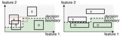
Figure 1: An example that we can obtain better model performance and cost-aware robustness if we use cost-driven constraints in robust training than $L_{\infty}$-norm bound. The dashed lines are the classification boundary. The left figure shows that robust training using $L_{\infty}$-norm bound (solid square box) achieves 75% accuracy. Given the cost-aware perturbation (dashed red rectangular box), the model has only 50% accuracy under attack. The right figure shows that using cost-driven constraint, we can achieve 100% accuracy with and without attack.

In this paper, we propose a systematic method to train cost-aware robust tree ensemble models for security, by integrating domain knowledge of feature manipulation cost. We first propose a cost modeling method that summarizes the domain knowledge about features into cost-driven constraint, which represents how bounded attackers can perturb every data point based on the cost of manipulating different features. Then, we integrate the constraint into the training process as if an arbitrary attacker under the cost constraint is trying to maximally degrade the quality of potential splits (Equation (8) in Section 3.2.2). We propose an efficient robust training algorithm that solves the maximization problem across different gain metrics and different types of models, including random forest model and gradient boosted decision trees. Lastly, we evaluate the adaptive attack cost against our robust training method, as a step towards understanding robustness against attacks in the problem space [45]. We propose an adaptive attack cost function to represent the total feature manipulation cost (Section 3.3), as the minimization objective of the strongest whitebox attacker against tree ensembles (the Mixed Integer Linear Program attacker). The attack objective specifically targets the cost-driven constraint, such that the attacker minimizes the total cost of perturbing different features.

Our robust training method incorporates the cost-driven constraint into the node construction process of growing trees, as shown in Figure 2. When any potential split $x^{j}<\eta$ (on the $j$-th feature) is being considered, due to the constraint, there is a range of possible values a data point can be changed into for that feature (formally defined in Section 3.1.1). Thus, data points close to the splitting threshold $\eta$ can potentially cross the threshold. For example, on a low cost feature, many data points can be easily perturbed to either the left child or the right child. Therefore, the constraint gives us a set of uncertain data points that can degrade the quality of the split, as well as high confidence data points that cannot be moved from the two children nodes. We need to quantify the worst quality of the split under the constraint, in order to compute the gain metric. To efficiently solve this, we propose a robust training algorithm that iteratively assigns training data points to whichever side of the split with the worse gain, regardless of the choice of the gain function and the type of tree ensemble model. As an example, we can categorize every feature into negligible, low, medium, or high cost to be increased and decreased by the attacker. Then, we use a high-dimensional box as the constraint. Essentially, the constraint gives the bounded attacker a larger increase (decrease) budget for features that are easier to increase (decrease), and smaller budget for more costly features. The cost-driven constraint helps the model learn robustness that can maximize the cost of evasion for the attacker. We have implemented our training method in the state-of-the-art tree ensemble learning libraries: gradient boosted decision trees in XGBoost [13] and random forest in scikit-learn [4].

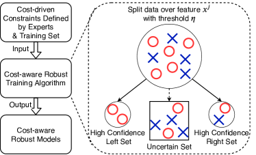
Figure 2: An overview of cost-aware robust tree ensemble training process. Our robust training algorithm incorporates the cost-driven constraint while constructing nodes. The constraint gives the set of data points that can potentially cross the split threshold $\eta$ given domain knowledge about the $j$-th feature, i.e. uncertain set.

We first evaluate the performance of our core training technique without the cost-driven constraint, against regular training method as well as the state-of-the-art robust tree ensemble training method from Chen et al. [11]. In the gradient boosted decision trees evaluation, we reproduce existing results to compare models over 4 benchmark datasets with the goal of improving robustness against attackers bounded by $L_{\infty}$-norm (Section 4.2). Using the same settings of number of trees and maximal depth hyperparameters from existing work, our robust training algorithm achieves on average 2.78$\times$ and 1.25$\times$ improvement over regular training and state-of-the-art robust training algorithm [11], respectively, in the minimal $L_{\infty}$ distance required to evade the model. In addition, we show that our algorithm provides better solutions to the optimization problem than the state-of-the-art [11] in 93% of the cases on average (Section 4.2.4).

In the random forest models evaluation, we have implemented Chen’s algorithm in scikit-learn since it was only available in XGBoost. We first train 120 models in total to perform grid search over number of trees and maximal depth hyperparameters. Then, we choose the hyperparameters with the best validation accuracy for each training algorithm and compare their robustness against the strongest whitebox attack. On average over the four benchmarking datasets, we achieve 3.52$\times$ and 1.7$\times$ robustness improvement in the minimal $L_{\infty}$ evasion distance compared to the baseline and Chen’s algorithm, repsectively. This shows that our core training technique alone has made significant improvements to solve the robust optimization problem.

Next, we evaluate the cost-aware robust training method for security, using Twitter spam URL detection as a case study. We reimplement the feature extraction over the dataset from [35] to detect malicious URLs posted by Twitter spammers. The features capture that attackers reuse hosting infrastructure resources, use long redirection chains across different geographical locations, and prefer flexibility of deploying different URLs. Based on domain knowledge, we specify four families of cost-driven constraints to train 19 different robust models, with key results summarized as follows. First, compared to regular training, our best model increases the cost-aware robustness by 10.6$\times$. Second, our robust training method using cost-driven constraints can achieve higher accuracy, lower false positive rate, and stronger cost-aware robustness than $L_{\infty}$-norm cost model from Chen’s algorithm [11]. Third, specifying larger perturbation range in the cost-driven constraint generally decreases accuracy and increases false positive rate; however, it does not necessarily increase the obtained robustness. We need to perform hyperparameter tuning to find the best cost model that balances accuracy and robustness. Lastly, by training cost-aware robustness, we can also increase the model’s robustness against $L_{1}$ and $L_{2}$ based MILP attacks [29].

Our contributions are summarized as the following:

• We propose a new cost modeling method to translate domain knowledge about features into cost-driven constraint. Using the constraint, we can train models to utilize domain knowledge outside the training data.

• We propose a new robust training algorithm to train cost-aware robust tree ensembles for security, by integrating the cost constraint. Our algorithm can be applied to both gradient boosted decision trees in XGBoost and random forest model in scikit-learn.

• We use Twitter spam detection as the security application to train cost-aware robust tree ensemble models. Compared to regular training, our best model increases the attack cost to evade the model by 10.6$\times$.

2 Background and Related Work

2.1 Tree Ensembles

A decision tree model guides the prediction path from the root to a leaf node containing the predicted value, where each internal node holds a predicate over some feature values. An ensemble of trees consists of multiple decision trees, which aggregates the predictions from individual trees. Popular aggregation functions include the average (random forest) and the sum (gradient boosted decision tree) of the prediction values from each decision tree.

2.1.1 Notations

We use the following notations for the tree ensemble in this paper. The training dataset $D$ has $N$ data points with $d$ features $D=\{(x_{i},y_{i})|i=1,2,...,N\}(x_{i}\in\mathbb{R}^{d},y\in\mathbb{R})$. Each input $x_{i}$ can be written as a $d$-dimensional vector, $x_{i}=[x_{i}^{1},x_{i}^{2},...,x_{i}^{d}]$. A predicate $p$ is in the form of $x^{j}<\eta$, which evaluates the $j$-th feature $x^{j}$ against the split threshold $\eta$. Specifically, for the i-th training data, the predicate checks whether $x_{i}^{j}<\eta$. If $p=true$, the decision tree guides the prediction path to the left child, otherwise to the right child. This process repeats until $x_{i}$ reaches a leaf. We use a function $f$ to denote a decision tree, which gives a real-valued output for the input data point $x$ with the true label $y$. For classification trees, $f(x)$ represents the predicted probability for the true label $y$.

The most common decision tree learning algorithms use a greedy strategy to construct the nodes from the root to the leaves, e.g., notably CART [8], ID3 [46], and C4.5 [47]. The algorithm greedily picks the best feature $j^{*}$ and the best split value $\eta^{*}$ for each node, which partitions the data points that reach the current node ($I$) to the left child ($I_{L}$) and the right child ($I_{R}$), i.e., $I=I_{L}\cup I_{R}$. The training algorithm optimizes the following objective using a scoring function to maximize the gain of the split:

$$j^{*},\eta^{*}=\operatorname*{arg\ max}_{j,\eta}Gain(I_{L},L_{R})=\operatorname*{arg\ max}_{j,\eta}(s(I)-s(I_{L},I_{R}))$$ (1)

In Equation (1), $s$ denotes a scoring function. For example, we can use Shannon entropy, Gini impurity, or any general loss function. Splitting a node changes the score from $s(I)$ to $s(I_{L},I_{R})$. For example, using the Gini impurity, we have $Gain(I_{L},L_{R})=Gini(I)-Gini(I_{L},I_{R})$. A common strategy to solve Equation (1) is to enumerate all the features with all the possible split points to find the maximum gain. Starting from the root node, the learning algorithm chooses the best feature split with the maximum gain, and then recursively constructs the children nodes in the same way, until the score does not improve or some pre-determined threshold (e.g., maximum depth) is reached.

A tree ensemble uses the weighted sum of prediction values from $K$ decision trees, where $K$ is a parameter specified by the user. Each decision tree can be represented as a function $f_{t}$. Then, the ensemble predicts the output $\hat{y}$ as follows.

$$\hat{y}=\phi(x)=a*\sum_{t=1}^{K}{f_{t}(x)}$$ (2)

Ensemble methods use bagging [7] or boosting [50, 21, 22] to grow the decision trees. Random forest and gradient boosted decision tree (GBDT) are the most widely used tree ensembles. The random forest model uses $a=\frac{1}{K}$, and the GBDT model set $a=1$. They use different methods to grow trees in parallel or sequentially, which we describe next.

2.1.2 Random Forest

A random forest model uses bagging [7] to grow the trees in parallel. Bagging, i.e., bootstrap aggregation, uses a random subset of the training data and a random subset of features to train individual learners. For each decision tree $f_{t}$, we first randomly sample $N^{\prime}$ data points from $D$ to obtain the training dataset $D_{t}=\{(x_{i},y_{i})\}$, where $|D_{t}|=N^{\prime}$ and $N^{\prime}\leq N$. Then, at every step of the training algorithm that solves Equation (1), we randomly select $d^{\prime}$ features in $I$ to find the optimal split, where $d^{\prime}\leq d$. The feature sampling is repeated until we finish growing the decision tree. The training data and feature sampling helps avoid overfitting of the model.

Random forest model has been used for various security applications, e.g., detecting malware distribution [34], malicious autonomous system [32], social engineering [42], phishing emails [20, 26, 16], advertising resources for ad blocker [28], and online scams [49, 31], etc. In some cases, researchers have analyzed the performance of the model (e.g., ROC curve) given different subsets of the features to reason about the predictive power of feature categories.

2.1.3 Gradient Boosted Decision Tree

Gradient boosted decision tree (GBDT) model uses boosting [50, 21, 22] to grow the trees sequentially. Boosting iteratively train the learners, improving the new learner’s performance by focusing on data that were misclassified by existing learners. Gradient boosting generalizes the boosting method to use an arbitrarily differentiable loss function.

In this paper, we focus on the state-of-the-art GBDT training system XGBoost [13]. When growing a new tree ($f_{t}$), all previous trees ($f_{1}$, $f_{2}$, …, $f_{t-1}$) are fixed. Using $\hat{y}^{(t)}$ to denote the predicted value at the t-th iteration of adding trees, XGBoost minimizes the regularized loss $\mathcal{L}^{(t)}$ for the entire ensemble, as the scoring function in Equation (1).

$$\mathcal{L}^{(t)}= \sum_{i=1}^{n}{l(y_{i},\hat{y}^{(t)}})+\sum_{i=1}^{t}\Omega(f_{i})$$ (3)

In the equation, $l$ is an arbitrary loss function, e.g., cross entropy; and $\Omega(f_{i})$ is the regularization term, which captures the complexity of the i-th tree, and encourages simpler trees to avoid overfitting. Using a special regularization term, XGBoost has a closed form solution to calculate the optimal gain of the corresponding best structure of the tree, given a split $I_{L}$ and $I_{R}$ as the following.

$$Gain(I_{L},L_{R})$$ (4)

$$=\frac{1}{2}\left[\frac{(\sum_{i\in I_{L}}g_{i})^{2}}{\sum_{i\in I_{L}}h_{i}+\lambda}+\frac{(\sum_{i\in I_{R}}g_{i})^{2}}{\sum_{i\in I_{R}}h_{i}+\lambda}-\frac{(\sum_{i\in I}g_{i})^{2}}{\sum_{i\in I}h_{i}+\lambda}\right]-\gamma$$

In particular, $g_{i}={\partial_{\hat{y}^{(t-1)}}}(l(y_{i},\hat{y}^{(t-1)})$ and $h_{i}={\partial_{\hat{y}^{(t-1)}}^{2}}(l(y_{i},\hat{y}^{(t-1)})$ are the first order and second order gradients for the $i$-th data point. In addition, $\gamma$ and $\lambda$ are hyperparameters related to the regularization term.

Boosting makes the newer tree dependent on previously grown trees. Previously, random forest was considered to generalize better than gradient boosting, since boosting alone could overfit the training data without tree pruning, whereas bagging avoids that. The regularization term introduced by xgboost significantly improves the generalization of GBDT.

2.2 Evading Tree Ensembles

There are several attacks against ensemble trees. Among the blackbox attacks, Cheng et al.’s attack [15] has been demonstrated to work on ensemble trees. The attack minimizes the distance between a benign example and the decision boundary, using a zeroth order optimization algorithm with the randomized gradient-free method. Papernot et al. [44] proposed a whitebox attack based on heuristics. The attack searches for leaves with different classes within the neighborhood of the targeted leaf of the benign example, to find a small perturbation that results in a wrong prediction. In this paper, we evaluate the robustness of a tree ensemble by analyzing the potential evasion caused by the strongest whitebox adversary, the Mixed Integer Linear Program (MILP) attacker. The adversary has whitebox access to the model structure, model parameters and the prediction score. The attack finds the exact minimal evasion distance to the model if an adversarial example exists.

Strongest whitebox attack: MILP Attack. Kantchelian et al. [29] have proposed to attack tree ensembles by constructing a mixed integer linear program, where the variables of the program are nodes of the trees, the objective is to minimize a distance (e.g., $L_{p}$ norm distance) between the evasive example and the attacked data point, and the constraints of the program are based on the model structure. The constraints include model mislabel requirement, logical consistency among leaves and predicates. Using a solver, the MILP attack can find adversarial example with the minimal evasion distance. Otherwise, if the solver says the program is infeasible, there truly does not exist an adversarial example by perturbing the attacked data point. Since the attack is based on a linear program, we can use it to minimize any objective in the linear form.

Adversarial training limitation. The MILP attack cannot be efficiently used for adversarial training, e.g., it can take up to an hour to generate one adversarial example [12] depending on the model size. Therefore, we integrate the cost-driven constraint into the training process directly to let the model learn knowledge about features. Moreover, Kantchelian et al. [29] demonstrated that adversarial training using a fast attack algroithm that hardens $L_{0}$ evasion distance makes the model weaker against $L_{1}$ and $L_{2}$ based attacks. Our results demonstrate that by training cost-aware robustness, we can also enhance the model’s robustness against $L_{1}$ and $L_{2}$ based attacks.

2.3 Related Work

From the defense side, existing robust trees training algorithms [6, 11, 53] focus on defending against $L_{p}$-norm bounded attackers, which may not capture the attackers’ capabilities in many applications. Incer et al. [27] train monotonic classifiers with the assumption that the cost of decreasing some feature values is much higher compared to increasing them, such that attackers cannot evade by increasing feature values. In comparison, we model difficulties in both increasing and decreasing feature values, since decreasing security features can incur costs of decreased utility [14, 30]. Zhang and Evans [56] are the first to train cost-sensitive robustness with regard to classification output error costs, since some errors have more catastrophic consequences than others [18]. Their work models the cost of classifier’s output, whereas we model the cost of perturbing the input features to the classifier.

The work most related to ours is from Calzavara et al. [9, 10]. They proposed a threat model that attackers can use attack rules, each associated with a cost, to exhaust an attack budget. The attack rules have the advantage of accurately perturbing categorical features by repeatedly corrupting a feature value based on a step size. Their training algorithm indirectly computes a set of data points that can be perturbed based on all the possible combinations of the rules, which in general needs enumeration and incurs an expensive computation cost. In comparison, we map each feature value to perturbed ranges, which directly derives the set of data points that can cross the splitting threshold at training time without additional computation cost. Our threat model has the same expressiveness as their rule-based model. For example, by specifying the same perturbation range for every feature, we can capture attackers bounded by $L_{\infty}$-norn and $L_{1}$-norm distances. We could also model attacks that change categorical features by using conditioned cost constraint for each category. In addition, we can easily incorporate our cost-driven constraints on top of state-of-the-art algorithm [53] to train for attack distance metrics with dependencies among feature, e.g., constrained $L_{1}$ and $L_{2}$ distances.

Researchers have also modeled the cost in the attack objective. Lowd and Meek [39] propose a linear attack cost function to model the feature importance. It is a weighted sum of absolute feature differences between the original data point and the evasive instance. We design adaptive attack objectives to minimize linear cost functions in a similar way, but we assign different weights to different feature change directions. Kulynych et al. [33] proposed to model attacker’s capabilities using a transformation graph, where each node is an input that the attacker can craft, and each directed edge represents the cost of transforming the input. Their framework can be used to find minimal-cost adversarial examples, if there is detailed cost analysis available for the atomic transformations represented by the edges.

Pierazzi et al. [45] proposed several problem-space constraints to generate adversarial examples in the problem space, e.g., actual Android malware. Their constraints are related to the cost factors we discuss for perturbing features. In particular, a high cost feature perturbation is more likely to violate their problem-space constraints, compared to a low cost change. For example, changes that may affect the functionality of a malware can violate the preserved semantics constraint, and attack actions that increases the suspiciousness of the malicious activity could violate the plausibility constraint. We could set a total cost budget for each category of the cost factors (similar to  [9, 10]), to ensure that problem-space constraints are not violated, which we leave as future work.

3 Methodology

In this section, we present our methodology to train robust tree ensembles that utilize expert domain knowledge about features. We will describe how to specify the attack cost-driven constraint that captures the domain knowledge, our robust training algorithm that use the constraint, and a new adaptive attack objective to evaluate the robust model.

3.1 Attack Cost-driven Constraint

3.1.1 Constraint Definition

We define the cost-driven constraint for each feature $x^{j}$ to be $C(x^{j})$. It is a mapping from the interval $[0,1]$, containing normalized feature values, to a set in $[0,1]\times[0,1]$. For each concrete value of $x^{j}$, $C(x^{j})$ gives the valid feature manipulation interval for any bounded attacker according to the cost of changing the feature, for all training data points.

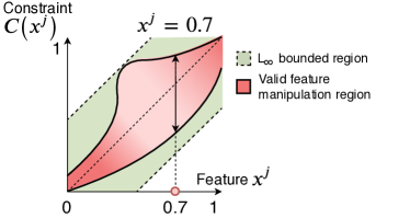
Figure 3: An example of cost-driven constraint for feature $x^{j}$. The red area represents valid feature manipulation region under the given cost-driven constraint $C(x^{j})$ while the green area represents the common $L_{\infty}$-norm bounded region. Lighter red color means lower cost region, such that these feature values can be perturbed more by the attacker. The $L_{\infty}$ region is imprecise to capture the cost.

Figure 3 shows two examples of cost-driven constraints. We use the shaded region within the dashed lines to denote the constraint when the attack cost is modeled by $L_{\infty}$-norm $\leq 0.5$ for feature $x^{j}$. As $x^{j}$ takes different feature values between 0 and 1, $L_{\infty}$ cost model states that the allowable perturbations for the feature are within $[x^{j}-0.5,x^{j}+0.5]$. However, this region can be imprecise according to the meaning of the feature. If the cost of changing feature $x^{j}$ is high when the value is close to 0 and 1, and relatively low in the middle, we could have a valid feature manipulation region represented by the red area enclosed in solid curves. When $x^{j}=0.7$ for one data point, the constraint says that the cost is acceptable for the attacker to perturb $x^{j}$ between 0.45 and 0.90. Lighter colored region allows larger perturbations than the darker colored region. In general, the constraint can be anything specified by the domain expert, by considering different cost factors.

3.1.2 Cost Factors

Different factors may affect the attack cost of feature perturbation, and provide some general guidelines in ranking the cost across features and their values.

Economic. The economic return on the attacker’s investment is a major motivation to whether they are willing to change some features. For example, to evade blocklist detection, the attackers constantly register new domains and rent new servers. Registering new domains is preferred since this costs less money than renting a new server.

Functionality. Some features are related to malicious functionalities of the attack. For example, the cryptojacking classifier [30] uses a feature that indicates whether the attack website calls the CryptoNight hashing function to mine Monero coins. Without function aliases, it is a high cost to remove the hash function since the website can no longer mine coins.

Suspiciousness. If the attacker needs to generate a lot more malicious activities to perturb features (e.g., sending more tweets than 99% of users), this makes the attack easier to be detected and has a cost.

Monotonicity. In security applications, the cost to increase a feature may be very different from decreasing it. For example, to evade malware detector that uses “static import” features, it is easier to insert redundant libraries than to remove useful ones [27]. Therefore, we need to specify the cost for both directions of the change.

Attack seed. If the attack starts modifying features from a benign example (e.g., reverse mimicry attack), the cost of changing features may be different from modifying features from a malicious data point. Therefore, the seed sample can affect the cost.

Ranking feature cost. Before specifying the constraints, we can roughly rank the cost of manipulating different features and different values of the same feature. All the cost factors can be translated to some return over investment for attackers. Perturbing a feature could cost the attacker more investment to set up the attack infrastructure, purchase more compromised machines, or obtain some expensive benign samples. On the other hand, feature perturbation could reduce the revenue of malicious activities by eliminating certain functionalities, or sacrificing some bots to be detected. From the perspective of both the investment and the return, a domain expert can rank features by attack costs, which is useful to construct the cost-driven constraint. In addition, we can use intervals or a continuous function of the value to rank the cost of perturbing different values for the same feature. Given the cost ranking of features, we provide two example constraints below.

3.1.3 Box Cost Constraint

As an example, we describe how to specify the box constraint to capture the domain knowledge about feature manipulation cost. After analyzing the cost factors and ranking the feature manipulation cost, we categorize attacker’s cost of increasing and decreasing the value of each feature into one of the four categories: negligible, low, medium, and high costs. The categories are based on relative cost differences, rather than absolute scale.

Negligible cost. There is negligible cost to perturb some features. For example, in the code transformation attack against authorship attribution classifier, the attacker can replace a for loop with a while loop without modifying any functionality of the code [48]. This changes the syntactic features of the classifier but incurs negligible costs.

Low and medium cost. Altering some features generates low or medium level of costs by comparison. For example, registering a new phishing domain name is generally considered to be lower cost for the attacker than renting and maintaining a new hosing server [37]. Therefore, increasing domain name count features can be categorized as low cost, whereas increasing IP address count features is medium cost.

High cost. If changing a feature significantly reduces the attack effectivenss, or compromises the attacker, then it is a high cost feature.

Box constraint. After assigning different categories to increasing/decreasing features, we can map the knowledge into a high dimensional box as the following.

$$C(x^{j})=[x^{j}-l_{j},x^{j}+h_{j}],\ j=1,2,3,...,d$$ (5)

It means that for the $j$-th feature, the constraint maps the feature to the interval $[x^{j}-l_{j},x^{j}+h_{j}]$ that represents the attacker’s allowable changes on the $j$-th feature value by decreasing or increasing it. According to the category of cost for decreasing and increasing the $j$-th feature, we can assign concrete values for $l_{j}$ and $h_{j}$. These values can be hyperparameters for the training procedure. Table 1 shows a mapping from the four categories to hyperparameters $\alpha,\beta,\gamma$, and $\mu$, representing the percentage of change with regard to the maximal value of the feature. A higher cost category should allow a smaller percentage of change than a lower cost category, and thus, $\mu<\gamma<\beta<\alpha$.

Cost	Value for $l_{j}$, $h_{j}$
Negligible	$\alpha$
Low	$\beta$
Medium	$\gamma$
High	$\mu$
Relationship	$\mu<\gamma<\beta<\alpha$

Table 1: Feature manipulation cost categories based on domain knowledge. For each feature $j$, we categorize the cost of increasing and decreasing its values and assign the bound for the box constraint using variables $l_{j}$ and $h_{j}$.

For each dimension $j$ of every training data point $x_{i}$, the constraint says that the attacker is allowed to perturb the value $x_{i}^{j}$ to $[x_{i}^{j}-l_{j},x_{i}^{j}+h_{j}]$. We will use this information to compute the gain of the split on $x^{j}$ in Equation (1). When comparing the quality of the splits, the cost-driven constraint changes how the gain is evaluated, which we will formalize in Equation (8). In particular, if a split threshold is within the perturbation interval, the training data point can be perturbed to cross the split threshold and potentially evade the classifier, which degrades the gain of the split.

3.1.4 Conditioned Cost Constraint

As another example, we can design the cost-driven constraint based on different conditions of the data point, e.g., the attack seed factor. In addition, the constraint can vary for different feature values. For example, we can design the constraint in Equation (6) where $x_{i}^{j}$ denotes the $j$-th feature value of data point $x_{i}$.

$$C(x_{i}^{j})=\begin{cases}0&x_{i}\ \text{is benign}\\ [x_{i}^{j},1]&x_{i}\ \text{is mal, pred score > 0.9}\\ [-0.1,0.1]*x_{i}^{j}&x_{i}\ \text{is mal, pred score <= 0.9}\\ \end{cases}$$ (6)

In this example, we give different constraints for benign and malicious data points for the $j$-th feature. If a data point $x_{i}$ is benign, we assign a value zero, meaning that it is extremely hard for the attacker to change the $j$-th feature value for a benign data point. If the data point is malicious, we separate to two cases. When the prediction score is higher than 0.9, we enforce that $x_{i}^{j}$ can only be increased. On the other hand, when the prediction score is less than or equal to 0.9, we allow a relative 10% change for both increase and decrease directions, depending on the original value of $x_{i}^{j}$.

When evaluating the gain of the split in the training process, we can use this constraint to derive the set of training data points under attack for every feature dimension $j$ and every split threshold $\eta$ as following. First, we calculate the prediction confidence of a training data point by using the entire tree model. If the prediction score is larger than 0.9, we take every malicious data point with $x_{i}^{j}<\eta$. Otherwise, we take all malicious data points with $x_{i}^{j}\in[\frac{1}{1.1}\eta,\frac{1}{0.9}\eta]$ to calculate the reduced gain of the split. We don’t consider benign data points to be attacked in this case.

Our threat model has the same expressiveness as the rule-based model in [10]. Our approach to use the cost driven constraint directly maps each feature value to perturbed ranges, which can be more easily integrated in the robust training algorithm compared to the rule-based threat model.

3.2 Robust Training

Given attack cost-driven constraints specified by domain experts, we propose a new robust training algorithm that can integrate such information into the tree ensemble models.

3.2.1 Intuition

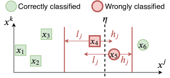
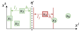
Figure 4: The intuition behind the attack cost-driven constraints for robust training, given six training points with two different classes (square and circle). It is easier to decrease $x^{j}$ than to increase it for the attacker. In the top figure, the split is 100% accurate without attacks, but only 66.6% accurate under attacks. The split in the bottom figure is always robust, but has a 83.3% accuracy.

Using the box constraint as an example, we present the intuition of our robust training algorithm in Figure 4. The regular training algorithm of tree ensemble finds a non-robust split (top), whereas our robust training algorithm can find a robust split (bottom) given the attack cost-driven constraint. Specifically in the example, it is easier to decrease the feature $x^{j}$ than to increase it. The cost constraint to increase (decrease) any $x^{j}$ is defined by $h_{j}$ ($l_{j}$). Here $x_{1},...,x_{6}$ are six training points with two different labels. The top of Figure 4 shows that, in regular training, the best split threshold $\eta$ over feature $x^{j}$ is between $x_{4}$ and $x_{5}$, which perfectly separates the data points into left and right sets. However, given the attack cost to change feature $x^{j}$, $x_{4}$ and $x_{5}$ can both be easily perturbed by the adversary and cross the splitting threshold $\eta$. Therefore, the worst case accuracy under attacks is 66.6%, although the accuracy is 100% without attacks. By integrating the attack cost-driven constraints, we can choose a more robust split, as shown in the bottom of Figure 4. Even though the attacker can increase $x_{3}^{j}$ by up to $h_{j}$, and decrease $x_{4}^{j}$ by up to $l_{j}$, the data points cannot cross the robust split threshold $\eta^{\prime}$. Therefore, the worst case accuracy under attacks is 83.3%, higher than that from the naive split. As a tradeoff, $x_{4}$ is wrongly separated without attacks, which results in 83.3% regular test accuracy as well. As shown in the figure, using a robust split can increase the minimal evasion distance for the attacker to cross the split threshold.

3.2.2 Optimization Problem

In robust training, we want to maximize the gain computed from potential splits (feature $j$ and threshold $\eta$), given the domain knowledge about how robust a feature $x^{j}$ is. We use $C$ to denote the attack cost-driven constraint. Following Equation (1), we have the following:

$$j^{*},\eta^{*} =\operatorname*{arg\ max}_{j,\eta}Gain(I_{L},L_{R},C)$$ (7)

$$=\operatorname*{arg\ max}_{j,\eta}(s(I,C)-s(I_{L},I_{R},C))$$

$$=\operatorname*{arg\ max}_{j,\eta}(s(I)-s(I_{L},I_{R},C))$$

Project constraint into set $\Delta I$. Since perturbing the feature does not change the score $s(I)$ before the split ($s(I,C)$ is the same as $s(I)$), this only affects the score $s(I_{L},I_{R},C)$ after the split, which cannot be efficiently computed. Therefore, we project the second term as the worst case score conditioned on some training data points $\Delta I$ being perturbed given the constraint function. The perturbations degrade the quality of the split to two children sets $I^{\prime}_{L}$ and $I^{\prime}_{R}$ that are more impure or with higher loss values. To best utilize the feature manipulation cost knowledge, we optimize for the maximal value of the score after the split, given different children sets $I^{\prime}_{L}$ and $I^{\prime}_{R}$ under the constraint. We then further categorize them into the high confidence points $I_{L_{c}}$ on the left side, $I_{R_{c}}$ on the right side, and low confidence points $\Delta I_{L}$ and $\Delta I_{R}$:

$$s(I_{L},I_{R},C) =\max_{I^{\prime}_{L},I^{\prime}_{R},C}s(I^{\prime}_{L},I^{\prime}_{R})$$ (8)

$$=\max_{\Delta I_{L},\Delta I_{R}}s(I_{L_{c}}\cup\Delta I_{L},I_{R_{c}}\cup\Delta I_{R})$$

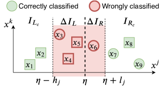
Figure 5: A simple example to illustrate the uncertain set $\Delta I=\Delta I_{L}\cup\Delta I_{R}=[x_{3},x_{4},x_{5},x_{6}]$ within the robust region $[\eta-h_{j},\eta+l_{j}]$ on feature $x^{j}$. The split threshold $\eta$ separates the data points into high confidence left set $I_{L_{c}}$ and high confidence right set $I_{R_{c}}$. Attackers can perturb the data points within the uncertain set $\Delta I_{L}\cup\Delta I_{R}$ to cross the split threshold, but not the high confidence data points.

Example. Different constraint functions result in different $\Delta I$ set. As an example, Figure 5 explains how we can map the box constraint for the $j$-th feature to an uncertain set $\Delta I$ containing variables to be optimized. We have nine data points numbered from 1 to 9, i.e. $I=\{x_{1},x_{2},...,x_{9}\}$, with two classes shaped in circles and squares. The training process tries to put the splitting threshold $\eta$ between every two consecutive data points, in order to find the split with maximum gain (Equation (1)). In Figure 5, the split value under consideration is between data points $x_{5}$ and $x_{6}$. The regular training process then computes the gain of the split based on $I_{L}=\{x_{1},x_{2},x_{3},x_{4},x_{5}\}$ and $I_{R}=\{x_{6},x_{7},x_{8},x_{9}\}$, using Equation 1. In the robust training process, we first project the box constraint for the feature $j$ into the uncertain set $\Delta I=\{x_{3},x_{4},x_{5},x_{6}\}$. Since the points on the left side of threshold $\eta$ can be increased by up to $h_{j}$, and points on the right side of $\eta$ can be decreased by up to $l_{j}$, we get the shaded region of $[\eta-h_{j},\eta+l_{j}]$ containing four data points that can be perturbed to cross the splitting threshold $\eta$. Then, we need to maximize the score after split under the box constraint. Each point in $\Delta I$ can be assigned to either the left side or the right side $\Delta I=\Delta I_{L}\cup\Delta I_{R}$, with $2^{|\Delta I|}$ possible assignments. Finding the minimal gain assignment is a combinatorial optimization problem, which needs to be repeatedly solved during the training process. Therefore, we propose a new algorithm to efficiently solve Equation (8).

3.2.3 Robust Training Algorithm

Algorithm 1 Robust Training Algorithm

Input: training set $D=\{(x_{i},y_{i})\},|D|=N$ $(x_{i}\in\mathbb{R}^{d},y\in\mathbb{R})$.

Input: data points of the current node $I=\{(x_{i},y_{i})\}$, $|I|=m$.

Input: attack cost-driven constraint $C$.

Input: the score function $s$.

Output: the best split at the current node $j^{*}$, $\eta^{*}$.

1:  Initialize $Gain^{*}=0;j^{*}=0;\eta^{*}=0$

2:  for $j=1$ to $d$ do

3:     Sort $I=\{(x_{i},y_{i})\}$ along the j-th feature as $\{(x_{t_{i}},y_{t_{i}})\}$

4:     for $t_{i}=t_{1}$ to $t_{m}$ do

5:        if $t_{i}=t_{1}$ then

6:           $\eta\leftarrow x_{t_{1}}^{j}$

7:        else

8:           $\eta\leftarrow\frac{1}{2}(x_{t_{i}}+x_{t_{i-1}})$

9:        end if

10:        Project $C$ to the uncertain set $\Delta I$.

11:        $I_{L}=\{(x_{i},y_{i})|x_{i}^{j}<\eta,x\notin\Delta I\}$

12:        $I_{R}=\{(x_{i},y_{i})|x_{i}^{j}>\eta,x\notin\Delta I\}$

13:        /* Greedily put $(x_{k},y_{k})$ to whichever side that has a larger score to solve Equation (8). */

14:        for every $(x_{k},y_{k})$ in $\Delta I$ do

15:           $ls=s(I_{L}\cup\{(x_{k},y_{k})\},I_{R})$

16:           $rs=s(I_{L},I_{R}\cup\{(x_{k},y_{k})\})$

17:           if $ls>rs$ then

18:              $I_{L}=I_{L}\cup\{(x_{k},y_{k})\}$

19:           else

20:              $I_{R}=I_{R}\cup\{(x_{k},y_{k})\}$

21:           end if

22:        end for

23:        /* Find the maximal gain. */

24:        $Gain(j,\eta,I)=s(I)-s(I_{L},I_{R})$

25:        if $Gain(j,\eta,I)>Gain^{*}$ then

26:           $j^{*}=j;\eta^{*}=\eta$

27:           $Gain^{*}=Gain(j,\eta,I)$

28:        end if

29:     end for

30:  end for

31:  return  $j^{*}$, $\eta^{*}$

We propose a new robust training algorithm to efficiently solve the optimization problem in Equation (8). Our algorithm works for different types of trees, including both classification and regression trees, different ensembles such as gradient boosted decision trees and random forest, and different splitting metrics used to compute the gain.

Algorithm 1 describes our robust training algorithm. The algorithm provides the optimal splitting feature $j^{*}$ and the splitting threshold $\eta^{*}$ as output. The input includes the training dataset, the set of data points that reach the current node $I=\{(x_{i},y_{i})\}$, the attack cost-driven constraint function, and a score function $s$. Example score functions are the cross-entropy loss, Gini impurity, or Shannon entropy. From Line 10 to Line 28, the algorithm does robust training, and the loops outside that are the procedure used in regular training algorithm. The algorithm marches through every feature dimension (the for loop at Line 2), to compute the maximal score after the split given the feature manipulation cost knowledge, for every possible split on that feature dimension. For each feature $j$, we first sort all the data points along that dimension (Line 3). Then, we go through all the sorted data points $(x_{t_{i}},y_{t_{i}})$ to consider the gain of a potential split $x^{j}<\eta$ where $\eta$ is calculated from Line 5 to Line 9. Given the constraint function C, we project that to the uncertain set $\Delta I$ and initialize two more sets: $I_{L}$ contains the data points that stay on the left side of the split, and $I_{R}$ contains the data points that stay on the right (Line 10 to 12). Next, from Line 13 to Line 22, we go through every uncertain data point, and greedily put it to either $I_{L}$ or $I_{R}$, whichever gives a larger score for the current split, to solve Equation (8) under attacks. After that, we compute the gain under attacks at Line 24, and update the optimal split $j^{*}$, $\eta^{*}$ for the current node if the current gain is the largest (Line 25 to 28). The algorithm eventually returns the optimal split ($j^{*}$, $\eta^{*}$) on Line 31.

3.3 Adaptive Attacker

To evaluate the robustness of the classifier against adaptive attacker, we define a new MILP attack objective, to minimize the following cost:

$$\text{minimize}\sum_{j}a_{j}w_{x^{j}}|\tilde{x}^{j}-x^{j}|+\sum_{j}(1-a_{j})w^{\prime}_{x^{j}}|\tilde{x}^{j}-x^{j}|$$ (9)

Where $a_{j}$ is defined as the following:

$$a_{j}=\begin{cases}0&\tilde{x}^{j}\leq x^{j}\\ 1&\tilde{x}^{j}>x^{j}\\ \end{cases}$$ (10)

The adaptive attacker wants to minimize the total feature manipulation cost to generate adversarial example $\tilde{x}$ by perturbing $x$. We model the total cost as the weighted sum of absolute feature value differences, with different weights for the increase and decrease changes. Each weight $w_{x^{j}}$ represents the unit cost (e.g., some dollar amount) for the attacker to increase feature $x^{j}$, and $w^{\prime}_{x^{j}}$ to decrease it.

To target the box cost constraint, we define $U_{N}$, $U_{L}$, $U_{M}$, and $U_{H}$ as the sets of feature dimensions with negligible, low, medium, and high cost to increase, respectively. We define $V_{N}$, $V_{L}$, $V_{M}$, and $V_{H}$ as the sets of feature dimensions with negligible, low, medium, and high cost to decrease, respectively. The adaptive attacker minimizes the following total feature manipulation cost:

$$\sum_{k}\sum_{U_{k}}w_{k}|\tilde{x}^{j}-x^{j}|+\sum_{k}\sum_{V_{k}}w_{k}|\tilde{x}^{j}-x^{j}|,k\in\{N,L,M,H\}$$ (11)

We set weights $w_{k}$ based on the inverse proportion of the box for each feature dimension, such that a larger weight prefers a smaller feature change in the attack. For example, if we allow perturbing a low cost feature to be twice the amount of a medium cost feature ($\beta=2*\gamma$) in the cost-driven constraint, we set $w_{L}=\frac{1}{2}w_{M}$, which makes the adaptive attacker aware that the cost of changing one unit of a medium cost feature is equivalent to changing two units of a low cost feature in the linear objective. This adapts the strongest whitebox attack by including the knowledge of box contraint used in the training.

4 Evaluation

In this section, we first evaluate the effectiveness of our core training algorithm (Section 4.2) against the state-of-the-art robust and regular training methods, and then we evaluate the end-to-end robust training technique on a security task, Twitter spam detection (Section 4.3).

4.1 Implementation

We implement our robust training algorithm in XGBoost [13] and scikit-learn [4]. Our implementation in XGBoost works with all their supported differentiable loss functions for gradient boosted decision trees as well as random forest. For scikit-learn, we implement the robust training algorithm in random forest using the Gini impurity score.

4.2 Training Algorithm Evaluation

Since the state-of-the-art training method [11] does not support integrating domain knowledge, we compare our core training algorithm (Algorithm 1) with $L_{\infty}$-norm cost model against existing work without any domain knowledge related cost modeling in this section. Even though it is unfair to our technique, the experiments in this section act as an ablation study to show the improvements our Algorithm 1 makes to solve Equation (8). Same as [11], we run our Algorithm 1 to train $L_{\infty}$-norm bounded robustness.

$L_{\infty}$ robustness definition. When the objective of the MILP attack (Section 2.2) is to minimize the $L_{\infty}$ distance, the attack provides the minimal $L_{\infty}$-norm evasion distance that the attacker needs to perturb in the features in order to evade the model. In non-security related applications, a larger $L_{\infty}$ robustness distance means that a model is more robust. For example, if the MNIST classifier requires an average of $0.3$ $L_{\infty}$-norm distance changes in adversarial examples, it is more robust than a model with $0.06$ $L_{\infty}$-norm robustness distance, because the adversarial examples look more differently from the original image.

Accuracy cutoff. In order to reproduce existing results in related work [11], we use $0.5$ prediction confidence as the cutoff to compute the accuracy scores for all trained models.

Dataset	Train set size	Test set size	Majority Class (%)	# of features
breast-cancer	546	137	62.64, 74.45	10
cod-rna	59,535	271,617	66.67, 66.67	8
ijcnn1	49,990	91,701	90.29, 90.50	22
MNIST 2 vs. 6	11,876	1,990	50.17, 51.86	784

Table 2: Training and testing set sizes, the percentage of majority class in the training and testing set, respectively, and the number of features for the four benchmark datasets.

4.2.1 Benchmark Datasets

We evaluate the robustness improvements in 4 benchmark datasets: breast cancer, cod-rna, ijcnn1, and binary MNIST (2 vs. 6). Table 2 shows the size of the training and testing data, the percentage of majority class in the training and testing set, respectively, and the number of features for these datasets. We describe the details of each benchmark dataset below.

Dataset	# of trees	Trained $\epsilon$		Tree Depth			Test ACC (%)			Test FPR (%)			Avg. $l_{\infty}$			Improv.
		Chen’s	ours	natural	Chen’s	ours	natural	Chen’s	ours	natural	Chen’s	ours	natural	Chen’s	ours	natural	Chen’s
breast-cancer	4	0.30	0.30	6	8	8	97.81	96.35	99.27	0.98	0.98	0.98	.2194	.3287	.4405	2.01x	1.34x
cod-rna	80	0.20	0.035	4	5	5	96.48	88.08	89.64	2.57	4.44	7.38	.0343	.0560	.0664	1.94x	1.19x
ijcnn1	60	0.20	0.02	8	8	8	97.91	96.03	93.65	1.64	2.15	1.62	.0269	.0327	.0463	1.72x	1.42x
MNIST 2 vs. 6	1,000	0.30	0.30	4	6	6	99.30	99.30	98.59	0.58	0.68	1.65	.0609	.3132	.3317	5.45x	1.06x

Table 3: Test accuracy and robustness of GBDT models trained by our algorithm (ours), compared to regularly trained models (natural) and the models trained by Chen and Zhang et al.’s method [11] (Chen’s), in XGBoost. The improvement (Improv.) here denotes the average $l_{\infty}$ robustness distance on our models over regularly trained ones and Chen and Zhang’s, by measuring adversarial examples found by Kantchelian’s MILP attack [29], the strongest whitebox attack.

breast cancer. The breast cancer dataset [1] contains 2 classes of samples, each representing benign and malignant cells. The attributes represent different measurements of the cell’s physical properties (e.g., the uniformity of cell size/shape).

cod-rna. The cod-rna dataset [2] contains 2 classes of samples representing sequenced genomes, categorized by the existence of non-coding RNAs. The attributes contain information on the genomes, including total free-energy change, sequence length, and nucleotide frequencies.

ijcnn1. The ijcnn1 dataset [3] is from the IJCNN 2001 Neural Network Competition. Each sample represents the state of a physical system at a specific point in a time series, and has a label indicating “normal firing" or “misfiring". We use the 22-attribute version of ijcnn1, which won the competition. The dataset has highly unbalanced class labels. The majority class in both train and test sets are 90% negatives.

MNIST 2 vs. 6. The binary mnist dataset [5] contains handwritten digits of “2" and “6". The attributes represent the gray levels on each pixel location.

Hyperparameters validation set. In the hyperparameter tuning experiments, we randomly separate the training set from the original data sources into a 90% train set and a 10% validation set. We use the validation set to evaluate the performance of the hyperparamters, and then train the model again using selected hyperparameters using the entire training set.

Robustness evaluation set. In order to reproduce existing results, we follow the same experiment settings used in [11]. We randomly shuffle the test set, and generate advesarial examples for 100 test data points for breast cancer, ijcnn1, and binary MNIST, and 5,000 test points for cod-rna.

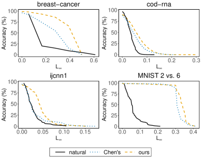
Figure 6: Accuracy under attack.

4.2.2 GBDT Results

We first evaluate the robustness of our training algorithm on the gradient boosted decision trees (GBDT) using the four benchmark datasets. We measure the model robustness using the $L_{\infty}$ evasion distance of the adversarial examples found by Kantchelian et al.’s MILP attack [29], the strongest whitebox attack that minimizes $L_{p}$-norm evasion distance for tree ensemble models. We compare the robustness achieved by our algorithm against regular training as well as the state-of-the-art robust training algorithm proposed by Chen et al. [11].

Hyperparameters. To reproduce the results from existing work [11] and conduct a fair comparison, we report results from the same number of trees, maximum depth, and $\epsilon$ for $L_{\infty}$-norm bound for regular training and Chen’s method in Table 3. For our own training method, we reused the same number of trees and maximum depth as Chen’s method. Then, we conducted grid search of different $\epsilon$ values by $0.01$ step size to find the model with the best accuracy. For our cod-rna model, we also experimented with $\epsilon$ values by $0.001$ step size. To further evaluate their choices of hyperparameters, we have conducted grid search for the number of trees and maximum depth to measure the difference in model accuracy, by training 120 models in total. Our results show that the hyperparameters used in existing work [11] produced similar accuracy as the best one (Appendix A.1). Note that the size of the breast-cancer dataset is very small (only 546 training data points), so using only four trees does not overfit the dataset.

Dataset	Trained $\epsilon$		Tree Num / Depth			Test ACC (%)			Test FPR (%)			Avg. $l_{\infty}$			Improv.
	Chen’s	ours	natural	Chen’s	ours	natural	Chen’s	ours	natural	Chen’s	ours	natural	Chen’s	ours	natural	Chen’s
breast-cancer	0.30	0.30	20 / 4	20 / 4	80 / 8	99.27	99.27	98.54	0.98	0.98	1.96	.2379	.3490	.3872	1.63x	1.11x
cod-rna	0.03	0.03	40 / 14	20 / 14	40 / 14	96.54	92.63	89.44	2.97	3.65	5.69	.0325	.0512	.0675	2.08x	1.32x
ijcnn1	0.03	0.03	100 / 14	100 / 12	60 / 8	97.92	93.86	92.26	1.50	0.78	0.08	.0282	.0536	.1110	3.94x	2.07x
MNIST 2 vs. 6	0.30	0.30	20 / 14	100 / 12	100 / 14	99.35	99.25	99.35	0.68	0.68	0.48	.0413	.1897	.2661	6.44x	1.40x

Table 4: Test accuracy and robustness of random forest models trained by our algorithm (ours) compared to regularly trained models (natural), in scikit-learn. The improvement (Improv.) here denotes the average $l_{\infty}$ robustness distance increase.

Minimal evasion distance. As shown in Table  3, our training algorithm can obtain stronger robustness than regular training and the state-of-the-art robust training method. On average, the MILP attack needs 2.78$\times$ larger $L_{\infty}$ perturbation distance to evade our models than regularly trained ones. Compared to the state-of-the-art Chen and Zhang et al.’s robust training method [11], our models require on average 1.25$\times$ larger $L_{\infty}$ perturbation distances. Note that the robustness improvement of our trained models are limited on binary MNIST dataset. This is because the trained and tested robustness ranges $L_{\infty}\leq 0.3$ are fairly large for MNIST dataset. The adversarial examples beyond that range are not imperceptible any more, and thus the robustness becomes extremely hard to achieve without heavily sacrificing regular accuracy.

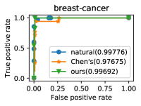
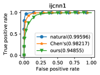
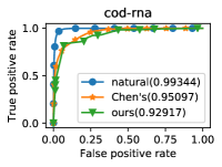
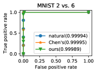
Figure 7: ROC curves of GBDT models trained with natural, Chen’s, and our training methods. AUC is given in the legend.

Accuracy under attack. Using the minimal $l_{\infty}$ evasion distances of adversarial examples, we plot how the accuracy of the models decrease as the attack distance increases in Figure 6. Compared to regular training, our models maintain higher accuracy under attack for all datasets except the breast-cancer one. Both breast-cancer models trained by our method and Chen’s method reach 0% accuracy at $l_{\infty}$ distance 0.5, whereas the largest evasion distance for the regularly trained model is 0.61. For the breast-cancer dataset, robustly trained models have an larger evasion distance than the regularly trained model for over 94% data points. Compared to Chen’s method, our models maintain higher accuracy under attack in all cases, except a small distance range for the ijcnn1 dataset ($l_{\infty}$ from 0.07 to 0.10, Figure 6).

Model quality evaluation. Figure 7 shows the ROC curves and the Area Under the Curve (AUC) for GBDT models trained with natural, Chen’s, and our training methods. For all the four testing datasets, the AUC of the model trained by our method is on par with the other two algorithms. On average, AUC of the model trained by our method is only 0.03 and 0.01 lower, while our method can increase the MILP attack cost by 2.78$\times$ and 1.25$\times$ than natural and Chen’s training methods, respectively. Table 3 shows that overall we maintain relatively high accuracy and low false positive rate. However, we have a high false positive rate for the cod-rna model and low accuray for the ijcnn1 model, as the tradeoff to obtain stronger robustness.

4.2.3 Random Forest Results

We evaluate the robustness of random forest models trained with our algorithm on the four benchmark datasets. We compare against Chen’s algorithm [11] and regular training in scikit-learn [4]. Since Chen’s algorithm is not available in scikit-learn, we have implemented their algorithm to train random forest models ourselves. We compare the effectiveness of our robust training algorithm against Chen’s method and regular training, when using Gini impurity to train random forest scikit-learn.

Hyperparameters. We conduct a grid search for the number of trees and maximum depth hyperparameters. Specifically, we use the following number of trees: 20, 40, 60, 80, 100, and the maximum depth: 4, 6, 8, 10, 12, 14. For each dataset, we train 30 models, and select the hyperparameters with the highest validation accuracy. The resulting hyperparameters are shown in Table 4. For the breast-cancer and binary mnist datasets, we re-used the same $\epsilon=0.3$ from Chen’s GBDT models. We tried different $L_{\infty}\leq\epsilon$ values of robust training for cod-rna and ijcnn1 datasets, and found out that $\epsilon=0.03$ gives a reasonable tradeoff between robustness and accuracy. For example, when $\epsilon=0.2$, we trained 30 random forest models using Chen’s method for the cod-rna dataset, and the best validation accuracy is only $79.5\%$. Whereas, using $\epsilon=0.03$ increases the validation accuracy to $91\%$.

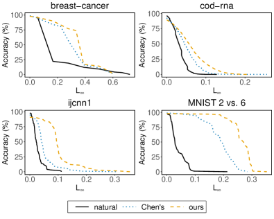
Figure 8: Accuracy under attack.

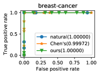
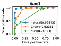
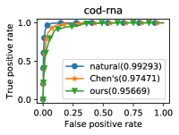
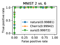
Figure 9: ROC curves of random forest models trained with natural, Chen’s, and our training methods in scikit-learn. AUC is given in the legend.

Minimal Evasion Distance. As shown in Table 4, the robustness of our random forest models outperforms the ones from regular training and Chen’s algorithm. Specifically, the average $l_{\infty}$ distance of adversarial examples against our robust models found by Kantchelian et al.’s MILP attack [29] is on average 3.52$\times$ and 1.7$\times$ larger than regular training and Chen’s method. On the other hand, there is only a $1.35\%$ average drop of test accuracy and under $3\%$ increase of false positive rate for the robust models compared to Chen’s method.

Accuracy under attack. Figure 8 shows the accuracy of models under different $L_{\infty}$ evasion distances of the MILP attack. Our models maintain higher accuracy under attack than those trained by Chen’s method for all datasets. In addition, our models maintain higher accuracy under attack than regular training, for all datasets except a small region for the breast-cancer dataset ($L_{\infty}>0.5$).

Model quality evaluation. Figure 9 shows the ROC curves and the Area Under the Curve (AUC) for random forest models trained with natural, Chen’s, and our training methods. For three datasets (breast-cancer, cod-rna, and binary MNIST), the ROC curve of our models are very close to the baseline models, with at most 0.018 drop in AUC than Chen’s method. However, our random forest model for the ijcnn1 dataset has very low AUC (0.74853). The model has 92% test accuracy, and the majority class of the test set is 90% negative class. Note that the false positive rate for the model is only 0.08% because the model does not predict the positive class very often, and therefore it generates very few false positives. We acknowledge the limitation of applying our algorithm in the $L_{\infty}$ norm cost model for the ijcnn1 dataset. This also motivates the need for cost models other than the $L_{\infty}$ norm. In Section 4.3.4, we demonstrate that we can balance robustness and accuracy using a cost model consistent with the semantics of the features for Twitter spam detection, even though using the $L_{\infty}$ cost model significantly degrades the model quality.

4.2.4 Benefits of our robust algorithm over existing heuristics

According to Equation (8), our robust algorithm is designed to maximize some impurity measure for each potential feature split during the training process. The higher the score is obtained by the algorithm, the stronger capability of the attacker is used for training, which guides the model to learn stronger robustness. Therefore, how well the algorithm can solve the maximization problem directly determines the eventual robustness the models can learn. To that end, we measure how our robust algorithm performs in solving the maximization problem compared to the heuristics used in state-of-the-art Chen and Zhang’s [11] to illustrate its effectiveness.

Dataset	Better (%)	Equal (%)	Worse (%)	Total
breast-cancer	99.74	0.26	0	3,047
cod-rna	94.13	4.66	1.21	35,597
ijcnn1	90.31	1.11	8.58	424,825
MNIST 2 vs. 6	87.98	6.33	5.69	796,264

Table 5: The percentage of the cases where our robust algorithm performs better, equally well, or worse than the heuristics used in the state-of-the-art Chen and Zhang et al.’s robust training algorithms [11] in solving the maximization problem (Equation 8). The total number of cases represent the total number of splits evaluated during robust optimization.

On the four benchmark datasets, we measure the percentage of the cases where our robust algorithms can better solve the maximization problem than the heuristics used in [11] and summarize the results in Table 5. The results show that our robust algorithm can provide a better solution than heuristics used in Chen and Zhang et al.’s method [11] for at least 87.98% cases during the whole training process. On small datasets like breast-cancer and cod-rna, our algorithm performs equally or better for 100% and 98.79% cases respectively. Such significant improvements in solving the maximizaation problem greatly benefit the robustness of our trained models. The results provide insights on why our robust training algorithm can obtain more robust tree ensembles than existing training methods.

4.3 Twitter Spam Detection Application

In this section, we apply our robust tree ensemble training method to a classic security application, spam URL detection on Twitter [35]. As a case study, we want to answer the following questions in the evaluation:

• Cost-driven constraint: How to specify the cost-driven constraint based on security domain knowledge? What is the advantage of training cost-driven constraint compared to $L_{\infty}$-norm robustness?

• Accuracy vs robustness tradeoffs: How much does robustness affect accuracy? Do different ways of specifying the cost-driven constraint change that tradeoffs?

• Adaptive attack cost: Against the strongest whitebox attack [29], does the robust model increase the adaptive attack cost for successful evasion?

• Other mathematical distances: Can we increase robustness against $L_{1}$ and $L_{2}$ based attacks?

4.3.1 Dataset

We obtain the public dataset used in Kwon et al.’s work [35] to detect spam URLs posted on Twitter. Spammers spread harmful URLs on social networks such as Twitter to distribute malware, scam, or phishing content. These URLs go through a series of redirections, and eventually reach a landing page containing harmful content. The existing detectors proposed in prior works often make decisions based on content-based features that are strong in predictive power but easy to be changed, e.g., different words used in the spam tweet. Kwon et al. propose to use more robust features that incur monetary or management cost to be changed under adversarial settings. They extract these robust features from the URL redirection chains (RC) and the corresponding connected components (CC) formed by the chains.

Dataset	Training	Testing
Malicious	130,794	55,732
Benign	165,076	71,070
Total	295,870	126,802

Table 6: The size of Twitter spam dataset [35].

Feature Name	Description	Cost
		$\downarrow$	$\uparrow$
Shared Resources-driven Features
EntryURLid	In degree of the largest redirector	M	N
AvgURLid	Average in degree of URL nodes in the RC	M	N
ChainWeight	Total frequency of edges in the RC	L	N
CCsize	# of nodes in the CC	L	N
CCdensity	Edge density of the CC	L	N
MinRCLen	Min length of the RCs in the CC	L	N
AvgLdURLDom	Average domain # of landing URL IPs in the CC	H	N
AvgURLDom	Average domain # for the IPs in the RC	M	N
Heterogeneity-driven Features
GeoDist	Total geo distance (km) traversed by the RC	H	N
CntContinent	# of unique continents in the RC	M	N
CntCountry	# of unique countries in the RC	M	N
CntIP	# of unique IPs in the RC	L	N
CntDomain	# of unique domains in the RC	L	N
CntTLD	# of unique TLDs in the RC	L	N
Flexibility Features
ChainLen	Length of the RC	L	N
EntryURLDist	Distance from the initial URL to the largest redirector	L	N
CntInitURL	# of initial URLs in the CC	L	N
CntInitURLDom	Total domain name # in the initial URLs	L	N
CntLdURL	# of final landing URLs in the RC	L	N
AvgIPperURL	Average IP # per URL in the RC	L	N
AvgIPperLdURL	Average IP # per landing URL in the CC	L	H
User Account Features
Mention Count	# of ‘@’ count to mention other users	N	L
Hashtag Count	# of hashtags	N	L
Tweet Count	# of tweets made by the user account	N	M
URL Percent	Percentage of user posts that contain a URL	N	L
$*$ CC: connected component. RC: redirection chain.
BPH: bulletproof hosting. N: Negligible. L: Low. M: Medium. H: High.

Table 7: We reimplement 25 features used in [35] to detect Twitter spam, among which three features have high cost to decrease or increase. To maintain the same level of spam activities, the attacker needs to purchase more bulletproof hosting servers to host the different landing pages if AvgLdURLDom feature is decreased or AvgIPperLdURL feature is increased. In addition, it is very hard for the attacker to decrease the GeoDist feature.

Feature extraction. We reimplemented and extracted 25 features from the dataset in the original paper, as shown in Table 7. There are four families of features: shared resources-driven, heterogeneity-driven, flexibility-driven, and user account and post level features. The key intuitions behind the features are as follows. 1) Attackers reuse underlying hosting infrastructure to reduce the economic cost of renting and maintaining servers. 2) Attackers use machines hosted on bulletproof hosting services or compromised machines to operate the spam campaigns. These machines are located around the world, which tend to spread over larger geographical distances than benign hosting infrastructure, and it is hard for attackers to control the geographic location distribution of their infrastructure. 3) Attackers want to maximize the flexibility of the spam campaign, so they use many different initial URLs to make the posts look distinct, and different domains in the long redirection chains to be agile against takedowns. 4) Twitter spammers utilize specific characters to spread harmful content, such as hashtags and ‘@’ mentions. We removed some highly correlated features from the original paper. For example, for a feature where the authors use both maximum and average numbers, we use the average number only.

Kwon et al. labeled the dataset by crawling suspended users, identifying benign users, and manually annotating tweets and URLs. In total, there are 186,526 distinct malicious tweets with spam URLs, and 236,146 benign ones. We randomly split the labeled dataset into 70% training set and 30% testing set as shown in Table 6. We extract the aforementioned 25 features from each data point and normalize the values to be between 0 and 1 for training and testing.

4.3.2 Attack Cost Analysis

In order to obtain the cost-driven constraint for robust training, we first analyze the cost of changing the features and the direction of the changes, then we specify a box contraint for the cost accordingly.

Feature Analysis

We categorize the features into negligible (N), low (L), medium (M), and high (H) cost to change, as shown in Table 7. We analyze the cost based on feature families as follows.

• Shared resources: All features cost more to be decreased than to be increased. If the attacker decreases the reused redirectors in the chain, the attacker needs to set up additional redirector servers to maintain the same level of spam activities (EntryURLid and AvgURLid features). It costs even more to set up more servers for the landing pages, since the landing URLs contain actual malicious content, which are usually hosted on bulletproof hosting (BPH) services. Feature AvgLdURLDom captures how the attacker is reusing the malicious content hosting infrastructure. If the value is decreased, the attacker will need to set up more BPH severs, which has the highest cost in the category.

• Heterogeneity: The total geographical distance traversed by the URL nodes in the redirection chain has the highest cost to change in general (GeoDist). If the attacker uses all the available machines as resources for malicious activities, it is hard to control the location of the machines and the distance between them. Overall, it is harder to decrease GeoDist to what looks more like benign value than to increase it. Since GeoDist values for benign URL redirection chains are very concentrated in one or two countries, the attacker would need to purchase more expensive resources located close by to mimic benign URL. The other four features that count number of continents, countries, IPs, domains, and top-level domains incur cost for decreased flexibility and increased maintainence cost if the features are decreased.

• Flexibility: All features in this family except the last one have relatively low cost to decrease, because that decreases the flexibility of the attack. The high cost feature AvgIPperLdURL counts the number of IP addresses that host the malicious landing page URL. If the attacker wants more flexibility of hosting the landing page on more BPH servers, the cost will be increased significantly.

• User account: Increasing features in this family generally increases suspiciousness of the user account. Among them, increasing the tweet count is the most suspicious of all, since a tweet is capped by 140 characters which limits the number of mentions and hashtags, and percentage of posts containing URLs is also capped. If a user account sends too many tweets that puts the account to the top suspicious percentile, it can be easily detected by simple filtering mechanism and compromise the account.

Overall, three features have the highest cost to be perturbed: AvgLdURLDom, GeoDist, and AvgIPperLdURL. Decreasing AvgLdURLDom and increasing AvgIPperLdURL incurs cost to obtain more bulletproof hosting servers for the landing page URL, and manipulating GeoDist is generally outside the control of the attacker. Other types of actions can also achieve the changes in AvgLdURLDom and AvgIPperLdURL, but it will generally decrease the profit of the malicious operation. To decrease AvgLdURLDom, if the attacker does not rent more BPH servers but only reduces the number of malicious landing pages, that reduces the profit. If the attacker increases the AvgIPperLdURL by using cheap servers, their malicious content could be taken down more often that interrupts the malicious operation.

Classifier Model	Constraint Variables				Adaptive Objective	Model Quality			Robustness against MILP
	N	L	M	H					Average
	$\alpha$	$\beta$	$\gamma$	$\mu$		Acc	FPR	AUC	$L_{1}$	$L_{2}$	$Cost_{1}$	$Cost_{2}$	$Cost_{3}$	$Cost_{4}$
Natural	-	-	-	-	-	99.38	0.89	.9994	.007	.006	.010	.009	.009	.008
C1 $\epsilon=0.03$	-	-	-	-	-	96.59	5.49	.9943	.046	.036	.080	.070	.062	.054
C2 $\epsilon=0.05$	-	-	-	-	-	94.51	7.27	.9910	.062	.053	.133	.109	.089	.085
C3 $\epsilon=0.1$	-	-	-	-	-	91.89	11.96	.9810	.079	.062	.156	.133	.111	.099
M1	0.08	0.04	0.02	0	$Cost_{1}$	98.24	2.05	.9984	.032	.027	.099	.051	.058	.056
M2	0.12	0.06	0.03	0		96.54	4.09	.9941	.043	.036	.106	.078	.064	.062
M3	0.20	0.10	0.05	0		96.96	4.10	.9949	.033	.027	.064	.025	.040	.040
M4	0.28	0.14	0.07	0		94.38	4.25	.9884	.024	.012	.043	.026	.039	.023
M5	0.32	0.16	0.08	0		93.85	9.62	.9877	.024	.015	.034	.025	.030	.025
M6	0.09	0.06	0.03	0.03	$Cost_{2}$	97.82	2.65	.9968	.049	.038	.104	.090	.070	.068
M7	0.15	0.10	0.05	0.05		96.60	4.91	.9929	.045	.039	.080	.072	.061	.060
M8	0.24	0.16	0.08	0.08		93.10	9.16	.9848	.041	.030	.082	.057	.050	.049
M9	0.30	0.20	0.10	0.10		92.28	12.16	.9836	.042	.028	.050	.044	.041	.038
M10	0.04	0.04	0.02	0	$Cost_{3}$	98.51	1.84	.9988	.025	.022	.087	.041	.052	.049
M11	0.06	0.06	0.03	0		97.31	3.65	.9953	.029	.017	.032	.027	.026	.025
M12	0.10	0.10	0.05	0		96.86	4.07	.9919	.044	.035	.062	.059	.049	.048
M13	0.16	0.16	0.08	0		94.54	5.91	.9900	.051	.041	.109	.090	.075	.074
M14	0.20	0.20	0.10	0		96.36	4.95	.9910	.033	.024	.054	.042	.043	.043
M15	0.28	0.28	0.14	0		93.81	6.57	.9851	.039	.039	.093	.070	.048	.048
M16	0.06	0.03	0.03	0	$Cost_{4}$	97.31	3.48	.9953	.036	.018	.038	.035	.034	.028
M17	0.10	0.05	0.05	0		97.41	2.70	.9964	.023	.020	.084	.034	.051	.049
M18	0.16	0.08	0.08	0		93.41	9.08	.9872	.035	.024	.074	.044	.062	.051
M19	0.20	0.10	0.10	0		96.48	4.75	.9918	.047	.038	.054	.041	.051	.051

Table 8: We trained classifiers with 19 different cost models under the box constraint, and we compare them against regular training (Natural) and three models from Chen’s method [11] with different $\epsilon$. We separate our models by four different cost families. Each cost family keeps the same proportion between the constraint variables and has the same adaptive attack objective. The best numbers within each cost family are highlighted in bold. We have also evaluated the recall of the models in Appendix A.2.

Objective	Adaptive Attack Weights
	$w_{N}$	$w_{L}$	$w_{M}$	$w_{H}$
$Cost_{1}$	1	2	4	$\infty$
$Cost_{2}$	1	2	3	3
$Cost_{3}$	1	1	2	$\infty$
$Cost_{4}$	1	2	2	$\infty$

Table 9: The weights in adaptive attack objective to target the four different families of cost models in Table 8.

4.3.3 Box Constraint Specification

We specify box constraint according to Section 3.1.3 with 19 different cost models as shown in Table 8, from M1 to M19. We want to allow more perturbations for lower cost features than higher cost ones, and more perturbations on the lower cost side (increase or decrease) than the higher cost side. According to Table 1 and our analysis of the features in Table 7, we assign the constraint variables $\alpha$, $\beta$, $\gamma$ and $\mu$ to negligible, low, medium, and high cost.

We specify four families of cost models, where each one has a corresponding adaptive attack cost to target the trained classifiers. We assign four distinct constraint variables in the first family (M1 to M5). For all the other families (M6 to M9, M10 to M15, and M16 to M19), we assign only three distinct constraint variables, representing three categories of feature manipulation cost, by repeating the same value for two out of four categories. For example, the second cost family (M6 to M9) merges medium and high cost categories into one using the same value for $\gamma$ and $\mu$. Within the same cost family, the relative scale of the constraint variables between the categories are the same, and the adaptive attack cost for that group is the inverse proportion of the constraint variables, as we have discussed in Section 3.3. For example, in the second group (M6 to M9), values for the low cost perturbation range ($\beta$) are twice the amount of the medium cost ones ($\gamma$), and the values for the negligible cost ($\alpha$) are three times of the medium cost ones ($\gamma$). Therefore, in the adaptive attack objective, we assign $w_{N}=1,w_{L}=2,w_{M}=3$ to capture that the cost of perturbing one, two, and three units of negligible, low, and medium cost features are equivalent. For each cost family, we vary the size of the bounding box to represent different attacker budget during training, resulting in 19 total settings of the constraint.

Using the cost-driven constraint, we train robust gradient boosted decision trees. We compare our training algorithm against regular training and Chen’s method [11]. We use 30 trees, maximum depth 8, to train one model using regular training. For Chen’s training algorithm, we specify three different $L_{\infty}$ norm cost models ($\epsilon=$ 0.03, 0.05, and 0.1) to obtain three models C1, C2, and C3 in Table 8. For Chen’s method and our own algorithm, we use 150 trees, maximum depth 24.

4.3.4 Results

Adaptive attack cost: Compared to regular training, our best model increases the cost-aware robustness by 10.6$\times$. From each cost family, our best models with the strongest cost-aware robustness are M2, M6, M13, and M19. Compared to the natural model obtained from regular training, our robust models increase the adaptive attack cost to evade them by 10.6$\times$ (M2, $Cost_{1}$), 10$\times$ (M6, $Cost_{2}$), 8.3$\times$ (M13, $Cost_{3}$), and 6.4$\times$ (M19, $Cost_{4}$), respectively. Thus, the highest cost-aware robustness increase is obtained by M2 model over the total feature manipulation cost $Cost_{1}$.

Advantages of cost-driven constraint: Our robust training method using cost-driven constraints can achieve stronger cost-aware robustness, higher accuracy, and lower false positive rate than $L_{\infty}$-norm cost model from Chen’s algorithm [11]. In Table 8, results from C1, C2, and C3 models demonstrate that if we use $L_{\infty}$-norm cost model ($L_{\infty}\leq\epsilon$), the performance of the trained model quickly degrades as $\epsilon$ gets larger. In particular, when $\epsilon=0.03$, the C1 model trained by Chen’s algorithm has decreased the accuracy to 96.59% and increased the false positive rate to 5.49% compared to regular training. With larger $\epsilon$ values, C2 and C3 models have even worse performance. C3 has only 91.89% accuracy and a very high 11.96% false positive rate. In comparison, if we specify attack cost-driven constraint in our training process, we can train cost-aware robust models with better performance. For example, our model M6 can achieve stronger robustness against cost-aware attackers with all four adaptive attack cost than C1. At the same time, M6 has higher accuracy and lower false positive rate than C1.

Robustness and accuracy tradeoffs: Training a larger bounding box generally decreases accuracy and increases false positive rate within the same cost family; however, the obtained robustness against MILP attacks vary across different cost families. Whenever we specify a new cost family with different constraint variable proportions and number of categories, we need to perform constraint parameter tuning to find the model that best balances accuracy and robustness.

• In the first cost family, as the bounding box size increases, the adaptive evasion cost $Cost_{1}$ against the models increases, and then decreases. M2 has the largest evasion cost.

• In the second cost family where we merge medium cost and high cost, the adaptive evasion cost $Cost_{2}$ decreases as the bounding box size increases.

• In the third cost family where we merge negligible cost and low cost, the adaptive evasion cost $Cost_{3}$ has high values for M10 and M13, and varies for other models.

• In the last cost family where we merge low cost and medium cost, the adaptive evasion cost $Cost_{4}$ increases as the bounding box size increases.

Other mathematical distances: Although our current implementation does not support training L1 and L2 attack cost models directly, training our proposed cost models can obtain robustness against L1 and L2 attacks. Comparing to the C1 model trained by Chen’s algorithm, we can obtain stronger robustness against L1 and L2 based MILP attacks while achieving better model performance. For example, our models M6 and M19 have larger L1/L2 evasion distance than C1, and they have lower false positive rate and higher/similar accuracy.

4.3.5 Discussion

Robustness and accuracy tradeoffs. Obtaining robustness of a classifier naturally comes with the tradeoff of decreased accuracy and increased false positive rate. We have experimented with 19 different cost models to demonstrate such tradeoffs in Table 8. In general, we need to perform constraint hyperparamters tuning to find the model that best balances accuracy, false positive rate, and robustness. In comparison with $L_{\infty}$ based cost models (C1, C2 and C3), we can achieve relatively higher accuracy and lower false positive rate while obtaining stronger robustness against cost-aware attackers (e.g., M6 vs C1). This is because $L_{\infty}$ based cost model allows attackers to perturb all features with equally large range, making it harder to achieve such robustness and easier to decrease the model performance. However, our cost-driven training technique can target the trained ranges according to the semantics of the features.

Scalability. For applications where thousands of features are used to build a classifier, we can categorize the features by semantics, and specify the cost-driven constraint as a function for different categories. Alternatively, we can also use $L_{\infty}$-norm as default perturbation for features, and specify cost-driven constraint for selected features.

Generalization. Our cost-aware training technique can generalize to any decision tree and tree ensemble training process, for both classification and regression tasks, e.g., AdaBoost [23] and Gradient Boosting Machine [24]. Since we apply the cost-aware constraint in the node splitting process, when constructing the classification and regression trees, we can calculate the maximal error of the split construction according to the allowable perturbations of the training data, and adjust the score for the split. This can be integrated in many different tree ensemble training algorithms. We leave investigation of integrating our technique to other datasets as future work.

5 Conclusion

In this paper, we have designed, implemented, and evaluated a cost-aware robust training method to train tree ensembles for security. We have proposed a cost modeling method to capture the domain knowledge about feature manipulation cost, and a robust training algorithm to integrate such knowledge. We have evaluated over four benchmark datasets against the regular training method and the state-of-the-art robust training algorithm. Our results show that compared to the state-of-the-art robust training algorithm, our model is 1.25$\times$ more robust in gradient boosted decision trees, and 1.7$\times$ more robust in random forest models, against the strongest whitebox attack based on $L_{p}$ norm. Using our method, we have trained cost-aware robust Twitter spam detection models to compare different cost-driven constraints. Moreover, one of our best robust models can increase the robustness by 10.6$\times$ against the adaptive attacker.

Appendix A Appendix

A.1 Hyperparameters for GBDT Models

To evaluate the hyperparameters for gradient boosted decision tree models used in [11], we train 35 models for each dataset to conduct a grid search. In details, we use maximum depth: 4, 5, 6, 7, 8, 9, 10; number of trees for breast-cancer: 2, 4, 6, 8, 10, cod-rna: 10, 20, 30, 40, ijcnn1: 20, 40, 60, 80, and binary mnist: 600, 800, 1000, 1200. Table 10 and 11 reports the model hyperparameters and corresponding test accuracy of trained models which obtain the best validation accuracy. In comparison with the results from Table 3, the hyperparameters used by [11] can train models with accuracy similar to the best one.

Dataset	Trained $\epsilon$		Tree Num / Depth
	Chen’s	ours	natural	Chen’s	ours
breast-cancer	0.30	0.30	4 / 6	4 / 4	2 / 7
cod-rna	0.20	0.03	40 / 10	40 / 4	10 / 10
ijcnn1	0.20	0.02	80 / 5	80 / 10	80 / 10
MNIST 2 vs. 6	0.30	0.30	600 / 4	600 / 8	600 / 9

Table 10: GBDT model hyperparameters with the best validation accuracy in XGBoost.

Dataset	Test ACC (%)			Test FPR (%)
	natural	Chen’s	ours	natural	Chen’s	ours
breast-cancer	97.81	96.35	99.27	0.98	0.98	0.98
cod-rna	96.74	87.32	91.08	2.79	4.05	8.71
ijcnn1	97.85	97.24	93.66	1.74	1.53	1.70
MNIST 2 vs. 6	99.70	99.65	99.55	0.39	0.39	0.29

Table 11: Test accuracy of GBDT models with the best validation accuracy in XGBoost.

A.2 Recall for Twitter Spam Models

To evaluate the performance of all 23 models trained to detect Twitter spam, we computed the recall at 1% FPR, 5% FPR, and 10% FPR in Table 12. The models M1, M6, M10, and M16 have the best recall within their cost family.

Classifier Model	Adaptive Objective	Model Quality
		1% FPR	5% FPR	10% FPR
		Recall	Recall	Recall
Natural	-	0.9974	0.9998	0.9999
C1	-	0.8177	0.9844	0.9999
C2	-	0.7912	0.9250	0.9897
C3	-	0.6928	0.8609	0.8609
M1	$Cost_{1}$	0.9612	0.9992	0.9997
M2		0.7949	0.9893	0.9973
M3		0.8214	0.9948	0.9981
M4		0.7537	0.9281	0.9689
M5		0.6907	0.9280	0.9840
M6	$Cost_{2}$	0.9162	0.9948	0.9968
M7		0.7881	0.9901	0.9959
M8		0.6793	0.9220	0.9608
M9		0.6780	0.9016	0.9386
M10	$Cost_{3}$	0.9715	0.9996	0.9999
M11		0.8671	0.9948	0.9991
M12		0.7484	0.9846	0.9930
M13		0.7753	0.9383	0.9896
M14		0.7473	0.9806	0.9925
M15		0.6728	0.8852	0.9862
M16	$Cost_{4}$	0.8624	0.9929	0.9989
M17		0.9061	0.9946	0.9973
M18		0.7075	0.9368	0.9749
M19		0.7298	0.9361	0.9703

Table 12: Recall at 1% FPR, 5% FPR, and 10% FPR for all Twitter spam detection models. The best recall numbers highlighted in bold.

References

- [1] Breast Cancer Wisconsin (Original) Data Set. https://archive.ics.uci.edu/ml/datasets/breast+cancer+wisconsin+(original).
- [2] Cod-RNA Data Set. https://www.csie.ntu.edu.tw/~cjlin/libsvmtools/datasets/binary.html#cod-rna.
- [3] Ijcnn1 Data Set. https://www.csie.ntu.edu.tw/~cjlin/libsvmtools/datasets/binary.html#ijcnn1.
- [4] scikit-learn: Machine Learning in Python. https://scikit-learn.org/.
- [5] The MNIST Database of Handwritten Digits. http://yann.lecun.com/exdb/mnist/.
- [6] M. Andriushchenko and M. Hein. Provably robust boosted decision stumps and trees against adversarial attacks. In Advances in Neural Information Processing Systems, pages 12997–13008, 2019.
- [7] L. Breiman. Bagging predictors. Machine learning, 24(2):123–140, 1996.
- [8] L. Breiman, J. Friedman, R. Olshen, and C. Stone. Classification and regression trees. Wadsworth Int Group, 37(15):237–251, 1984.
- [9] S. Calzavara, C. Lucchese, and G. Tolomei. Adversarial training of gradient-boosted decision trees. In Proceedings of the 28th ACM International Conference on Information and Knowledge Management, pages 2429–2432, 2019.
- [10] S. Calzavara, C. Lucchese, G. Tolomei, S. A. Abebe, and S. Orlando. Treant: training evasion-aware decision trees. Data Mining and Knowledge Discovery, pages 1–31, 2020.
- [11] H. Chen, H. Zhang, D. Boning, and C.-J. Hsieh. Robust decision trees against adversarial examples. In International Conference on Machine Learning (ICML), 2019.
- [12] H. Chen, H. Zhang, S. Si, Y. Li, D. Boing, and C.-J. Hsieh. Robustness verification of tree-based models. In Advances in Neural Information Processing Systems, 2019.
- [13] T. Chen and C. Guestrin. Xgboost: A scalable tree boosting system. In Proceedings of the 22nd acm sigkdd international conference on knowledge discovery and data mining, pages 785–794. ACM, 2016.
- [14] Y. Chen, Y. Nadji, A. Kountouras, F. Monrose, R. Perdisci, M. Antonakakis, and N. Vasiloglou. Practical attacks against graph-based clustering. In Proceedings of the 2017 ACM SIGSAC Conference on Computer and Communications Security, pages 1125–1142. ACM, 2017.
- [15] M. Cheng, T. Le, P.-Y. Chen, J. Yi, H. Zhang, and C.-J. Hsieh. Query-efficient hard-label black-box attack: An optimization-based approach. In International Conference on Learning Representations (ICLR), 2019.
- [16] A. Cidon, L. Gavish, I. Bleier, N. Korshun, M. Schweighauser, and A. Tsitkin. High precision detection of business email compromise. In 28th USENIX Security Symposium (USENIX Security 19), pages 1291–1307, 2019.
- [17] J. M. Cohen, E. Rosenfeld, and J. Z. Kolter. Certified adversarial robustness via randomized smoothing. arXiv preprint arXiv:1902.02918, 2019.
- [18] T. Dreossi, S. Jha, and S. A. Seshia. Semantic adversarial deep learning. arXiv preprint arXiv:1804.07045, 2018.
- [19] K. Dvijotham, S. Gowal, R. Stanforth, R. Arandjelovic, B. O’Donoghue, J. Uesato, and P. Kohli. Training verified learners with learned verifiers. arXiv preprint arXiv:1805.10265, 2018.
- [20] I. Fette, N. Sadeh, and A. Tomasic. Learning to detect phishing emails. In Proceedings of the 16th international conference on World Wide Web, pages 649–656. ACM, 2007.
- [21] Y. Freund. Boosting a weak learning algorithm by majority. Information and computation, 121(2):256–285, 1995.
- [22] Y. Freund and R. E. Schapire. A decision-theoretic generalization of on-line learning and an application to boosting. Journal of computer and system sciences, 55(1):119–139, 1997.
- [23] J. Friedman, T. Hastie, R. Tibshirani, et al. Additive logistic regression: a statistical view of boosting (with discussion and a rejoinder by the authors). The annals of statistics, 28(2):337–407, 2000.
- [24] J. H. Friedman. Greedy function approximation: a gradient boosting machine. Annals of statistics, pages 1189–1232, 2001.
- [25] S. Gowal, K. Dvijotham, R. Stanforth, R. Bunel, C. Qin, J. Uesato, T. Mann, and P. Kohli. On the effectiveness of interval bound propagation for training verifiably robust models. arXiv preprint arXiv:1810.12715, 2018.
- [26] G. Ho, A. Cidon, L. Gavish, M. Schweighauser, V. Paxson, S. Savage, G. M. Voelker, and D. Wagner. Detecting and characterizing lateral phishing at scale. In 28th USENIX Security Symposium (USENIX Security 19), pages 1273–1290, 2019.
- [27] I. Incer, M. Theodorides, S. Afroz, and D. Wagner. Adversarially robust malware detection using monotonic classification. In Proceedings of the Fourth ACM International Workshop on Security and Privacy Analytics, pages 54–63. ACM, 2018.
- [28] U. Iqbal, P. Snyder, S. Zhu, B. Livshits, Z. Qian, and Z. Shafiq. Adgraph: A graph-based approach to ad and tracker blocking. In Proc. of IEEE Symposium on Security and Privacy, 2020.
- [29] A. Kantchelian, J. Tygar, and A. Joseph. Evasion and hardening of tree ensemble classifiers. In International Conference on Machine Learning, pages 2387–2396, 2016.
- [30] A. Kharraz, Z. Ma, P. Murley, C. Lever, J. Mason, A. Miller, N. Borisov, M. Antonakakis, and M. Bailey. Outguard: Detecting in-browser covert cryptocurrency mining in the wild. In The World Wide Web Conference, pages 840–852, 2019.
- [31] A. Kharraz, W. Robertson, and E. Kirda. Surveylance: automatically detecting online survey scams. In 2018 IEEE Symposium on Security and Privacy (SP), pages 70–86. IEEE, 2018.
- [32] M. Konte, R. Perdisci, and N. Feamster. Aswatch: An as reputation system to expose bulletproof hosting ases. ACM SIGCOMM Computer Communication Review, 45(4):625–638, 2015.
- [33] B. Kulynych, J. Hayes, N. Samarin, and C. Troncoso. Evading classifiers in discrete domains with provable optimality guarantees. arXiv preprint arXiv:1810.10939, 2018.
- [34] B. J. Kwon, J. Mondal, J. Jang, L. Bilge, and T. Dumitraş. The dropper effect: Insights into malware distribution with downloader graph analytics. In Proceedings of the 22nd ACM SIGSAC Conference on Computer and Communications Security, pages 1118–1129. ACM, 2015.
- [35] H. Kwon, M. B. Baig, and L. Akoglu. A domain-agnostic approach to spam-url detection via redirects. In Pacific-Asia Conference on Knowledge Discovery and Data Mining, pages 220–232. Springer, 2017.
- [36] M. Lecuyer, V. Atlidakis, R. Geambasu, D. Hsu, and S. Jana. Certified robustness to adversarial examples with differential privacy. In 2019 IEEE Symposium on Security and Privacy (SP), pages 656–672. IEEE, 2019.
- [37] K. Levchenko, A. Pitsillidis, N. Chachra, B. Enright, M. Félegyházi, C. Grier, T. Halvorson, C. Kanich, C. Kreibich, H. Liu, et al. Click trajectories: End-to-end analysis of the spam value chain. In 2011 ieee symposium on security and privacy, pages 431–446. IEEE, 2011.
- [38] B. Li, C. Chen, W. Wang, and L. Carin. Second-order adversarial attack and certifiable robustness. 2018.
- [39] D. Lowd and C. Meek. Adversarial Learning. In Proceedings of the eleventh ACM SIGKDD international conference on Knowledge discovery in data mining, pages 641–647. ACM, 2005.
- [40] A. Madry, A. Makelov, L. Schmidt, D. Tsipras, and A. Vladu. Towards deep learning models resistant to adversarial attacks. International Conference on Learning Representations (ICLR), 2018.
- [41] M. Mirman, T. Gehr, and M. Vechev. Differentiable abstract interpretation for provably robust neural networks. In International Conference on Machine Learning (ICML), pages 3575–3583, 2018.
- [42] T. Nelms, R. Perdisci, M. Antonakakis, and M. Ahamad. Towards measuring and mitigating social engineering software download attacks. In 25th USENIX Security Symposium (USENIX Security 16), pages 773–789, 2016.
- [43] M. Norouzi, M. Collins, M. A. Johnson, D. J. Fleet, and P. Kohli. Efficient non-greedy optimization of decision trees. In Advances in neural information processing systems, pages 1729–1737, 2015.
- [44] N. Papernot, P. McDaniel, and I. Goodfellow. Transferability in machine learning: from phenomena to black-box attacks using adversarial samples. arXiv preprint arXiv:1605.07277, 2016.
- [45] F. Pierazzi, F. Pendlebury, J. Cortellazzi, and L. Cavallaro. Intriguing properties of adversarial ml attacks in the problem space. In 2020 IEEE Symposium on Security and Privacy (SP), pages 1332–1349. IEEE, 2020.
- [46] J. R. Quinlan. Induction of decision trees. Machine learning, 1(1):81–106, 1986.
- [47] J. R. Quinlan. C 4.5: Programs for machine learning. The Morgan Kaufmann Series in Machine Learning, 1993.
- [48] E. Quiring, A. Maier, and K. Rieck. Misleading authorship attribution of source code using adversarial learning. In 28th USENIX Security Symposium (USENIX Security 19), pages 479–496, 2019.
- [49] M. Z. Rafique, T. Van Goethem, W. Joosen, C. Huygens, and N. Nikiforakis. It’s free for a reason: Exploring the ecosystem of free live streaming services. In Proceedings of the 23rd Network and Distributed System Security Symposium (NDSS 2016), pages 1–15. Internet Society, 2016.
- [50] R. E. Schapire. The strength of weak learnability. Machine learning, 5(2):197–227, 1990.
- [51] A. Sinha, H. Namkoong, and J. Duchi. Certifying some distributional robustness with principled adversarial training. International Conference on Learning Representations (ICLR), 2018.
- [52] S. Wang, Y. Chen, A. Abdou, and S. Jana. Mixtrain: Scalable training of formally robust neural networks. arXiv preprint arXiv:1811.02625, 2018.
- [53] Y. Wang, H. Zhang, H. Chen, D. Boning, and C.-J. Hsieh. On -norm robustness of ensemble stumps and trees. In International Conference on Machine Learning (ICML), 2020.
- [54] E. Wong and Z. Kolter. Provable defenses against adversarial examples via the convex outer adversarial polytope. In International Conference on Machine Learning, pages 5283–5292, 2018.
- [55] E. Wong, F. Schmidt, J. H. Metzen, and J. Z. Kolter. Scaling provable adversarial defenses. Advances in Neural Information Processing Systems (NIPS), 2018.
- [56] X. Zhang and D. Evans. Cost-Sensitive Robustness against Adversarial Examples. International Conference on Learning Representations (ICLR), 2019.