Large-scale Multi-view Subspace Clustering in Linear Time

Abstract

A plethora of multi-view subspace clustering (MVSC) methods have been proposed over the past few years. Researchers manage to boost clustering accuracy from different points of view. However, many state-of-the-art MVSC algorithms, typically have a quadratic or even cubic complexity, are inefficient and inherently difficult to apply at large scales. In the era of big data, the computational issue becomes critical. To fill this gap, we propose a large-scale MVSC (LMVSC) algorithm with linear order complexity. Inspired by the idea of anchor graph, we first learn a smaller graph for each view. Then, a novel approach is designed to integrate those graphs so that we can implement spectral clustering on a smaller graph. Interestingly, it turns out that our model also applies to single-view scenario. Extensive experiments on various large-scale benchmark data sets validate the effectiveness and efficiency of our approach with respect to state-of-the-art clustering methods.

Introduction

During the last decade, subspace clustering has been explored extensively due to its promising performance (?; ?). Basically, it is based on the assumption that the data points are drawn from multiple low-dimensional subspaces and each group fits into one of the low-dimensional subspaces. Significant progress has been made to uncover such underlying subspaces.

Among the various subspace clustering approaches, spectral clustering based methods such as low-rank representation (LRR) (?; ?) and sparse subspace clustering (SSC) (?) have achieved great success. SSC finds a sparse representation of data points while LRR finds the low-rank structure of subspace. Afterwards, the spectral clustering algorithm is performed on such new representation (?). For $n$ data points, the first step typically takes $\mathcal{O}(n^{2})$ or $\mathcal{O}(n^{3})$ time while the second step requires $\mathcal{O}(n^{3})$ or at least $\mathcal{O}(n^{2}k)$ time, where $k$ is the number of clusters. Therefore, these two time comsuming steps debar the application of subspace clustering from large-scale data sets.

Recently, much work have been developed to accelerate subspace clustering. For example, (?) proposes a data selection approach; a scalable SSC based on orthogonal matching pursuit is developed in (?); a fast solver for SSC is proposed in (?); accelerated LRR is also developed (?; ?); a sampling approach is used in (?). Unfortunately, they all target for single-view scenario and can not deal with multi-view data.

With the advance of information technology, many practical data come from multiple channels or appear in muliple modalities, i.e., the same object can be described in different kinds of features (?; ?; ?; ?; ?; ?). Different feature sets often characterize different yet complementary information. For instance, an image can have heterogeneous features, such as Garbor, HoG, SIFT, GIST, and LBP; an artical can be written in different languages. Accordingly, it is crucial to develop multi-view learning method to incorporate the useful informaiton from different views.

There has been growing interest in developing multi-view subspace clustering (MVSC) algorithms. For example, MVSC (?) method learns a graph representation for each view and all graphs are assumed to share a unique cluster matrix; (?) applies a diversity term to explore the complementarity information; (?) explores both consistency and specificity of different views; (?; ?) perform MVSC in latent representation; (?) imposes both low-rank and sparsity constraints on the graph; (?; ?) learn one partition for each view and them perform a fusion in partition space. In terms of clustering accuracy, these methods are attractive. Nevertheless, their computation efficiency, at least $\mathcal{O}(n^{2}k)$ complexity, is largely ignored. In the era of big data, it has been witnessed that many applications involve large-scale multi-view data. Therefore, their severely unaffordable complexity precludes MVSC from real-world applications with big data. Moreover, existing single-view subspace clustering acceleration techniques do not apply to multi-view scenarios owing to the heterogeneous nature of multi-view data.

To fill the gap, we need to address two challenges. First, how to avoid constructing $n\times n$ graph for multi-view data, which requires a lot of time and storage. Second, how to circumvent the computationally expensive step—–spectral clustering with $\mathcal{O}(n^{2}k)$ complexity. To this end, we introduce a novel large-scale multi-view subspace clustering (LMVSC) method, which can greatly reduce the computational complexity as well as improve the clustering performance. First, to address the large-scale graph construction problem, we select a small number of the instances as anchors, and then a smaller graph is built for each view. Second, a novel way to integrate mutiple graphs is designed so that we can implement spectral clustering on a small graph.

The contributions of this paper mainly include：

• We make the first attempt towards large-scale multi-view subspace clustering. Our proposed method can be solved in linear time, while existing methods demand square or cubic time in the number of data instance.

• Extensive experiments in terms of data sets and comparison methods validate the effectiveness and efficiency of the proposed algorithm.

• As a special case, our method also applies to single-view subspace clustering task. It gives promising performance on very large-scale data.

Preliminaries

Multi-view Subspace Clustering

Subspace clustering expresses each data point as a linear combination of other points and minimizes the reconstruction loss to obtain the combination coefficient. This coefficient is treated as the similarity between corresponding points. Mathematically, given data $X\in\mathcal{R}^{d\times n}$ with $d$ features and $n$ samples, subspace clustering solves the following problem (?; ?; ?):

$$\min_{Z}\|X-XS\|_{F}^{2}+\alpha f(S)\quad s.t.\quad S\geq 0,\hskip 2.84544ptS\textbf{1}=\textbf{1},$$ (1)

where $f(\cdot)$ is a certain regularizer function, $\alpha>0$ is a balance parameter, and 1 is a vector with all ones. The constraints require that all $S_{ij}$ is nonnegative and $\sum_{j}S_{ij}=1$. $S$ is often called similarity graph matrix. It is obvious that $S$ has size of $n\times n$, which poses a big challenge with scalability to large-scale data sets.

Recently, multi-view subspace clustering (MVSC) has attracted much attention. Basically, for multi-view data $X=[X^{1};\cdots;X^{i};\cdots;X^{v}]\in\mathcal{R}^{\sum\limits_{i=1}^{v}d_{i}\times n}$, MVSC (?; ?; ?) solves:

$$\min_{S^{i}}\sum\limits_{i=1}^{v}\|X^{i}-X^{i}S^{i}\|_{F}^{2}+\alpha f(S^{i})\hskip 4.26773pts.t.\hskip 4.26773ptS^{i}\geq 0,\hskip 2.84544ptS^{i}\textbf{1}=\textbf{1}.$$ (2)

With different forms of $f$, Eq. (2) gives solutions with different properties. For example, (?) encourages similarity between pairs of graphs; (?) emphasizes the complementarity. With these multiple graphs, (?) assumes they produce the same clustering; (?; ?) perform spectral clustering on averaged graph. All these MVSC methods take at least $\mathcal{O}(n^{2}k)$ time, hence they are generally computational prohibtive.

Anchor Graph

Anchor graph is an efficient way to construct the large-scale graph matrix (?; ?; ?; ?). Specifically, a subset of $m$ points $(m\ll n)$ $A=[a_{1},a_{2},\cdots,a_{m}]\in\mathcal{R}^{d\times m}$ are chosen based on a $k$-means clustering or random sampling on the original data set. Each point plays a role as a landmark which approximates the neighborhood structure. Then, a sparse affinity matrix $Z\in\mathcal{R}^{n\times m}$ is constructed between the landmarks and the original data as follows:

$$Z_{ij}=\begin{cases}\frac{K_{\delta}(x_{i},a_{j})}{\sum_{j^{\prime}\in<i>}K_{\delta}(x_{i},a_{j^{\prime}})},&j\in<i>\\ 0,&\text{otherwise}\end{cases}$$ (3)

where $<i>$ indicates the indexes of $r$ $(r<m)$ nearest anchors around $x_{i}$. The function $K_{\delta}(\cdot)$ is the commonly used Gaussian kernel with bandwidth parameter $\delta$. Subsequently, the doubly-stochastic similarity matrix $S\in\mathcal{R}^{n\times n}$, the summation of each column and each row equal to one, is built based on:

$$S=\hat{Z}\hat{Z}^{\top}\quad\textit{where}\quad\hat{Z}=Z\Sigma^{-1/2},$$ (4)

where $\Sigma$ is a diagonal matrix with the entry $\Sigma_{ii}=\sum_{j=1}^{n}Z_{ji}$.

We can see that the above graph construction approach is extremely efficient since only $\mathcal{O}(mn)$ distances are considered. However, this heuristic strategy has one inherent drawback which is always ignored, i.e., quality of the built graph heavily depends on the exponential function. In general, it might not be appropriate to the structure of the data space (?; ?). Furthermore, it is also challenging to find a good kernel parameter without any supervision information. Consequently, the downstream task might not be able to obtain a good performance.

To obtain a similarity measure tailored to the problem at hand, a principled way is to learn it from data (?). In this paper, inspired by the idea of anchor graph, we use a smaller graph $Z$ to approximate the full $n\times n$ graph matrix. Different from existing approach, we adaptively learn $Z$ from raw data by solving an optimization problem.

Methodology

For large-scale data, there is much redundancy in the data; a small number of the instances are sufficient for reconstructing the underlying subspaces. Similar to anchor strategy, we use a smaller matrix $Z^{i}\in\mathcal{R}^{n\times m}(m\ll n)$ to approximate the full $n\times n$ matrix $S^{i}$. Specifically, a set of $m$ landmarks $A^{i}=\{a_{j}\}_{j\in[1,m]}$ (cluster centers) are obtained through $k$-means clustering on the data $X^{i}$. Then, $Z^{i}$ is built between the landmarks $A^{i}$ and $X^{i}$.

Rather than using the handcrafted similarity measure (3), we learn $Z^{i}$ from data. For multi-view data, we solve the following problem:

$$\begin{split}\min_{Z^{i}}&\sum_{i=1}^{v}\|X^{i}-A^{i}(Z^{i})^{\top}\|_{F}^{2}+\alpha\|Z^{i}\|_{F}^{2}\\ &s.t.\hskip 4.26773pt0\leq Z^{i},\hskip 2.84544pt(Z^{i})^{\top}\textbf{1}=\textbf{1}.\end{split}$$ (5)

Compared to Eq. (2), we only consider the similarities between $mn$ points instead of $n^{2}$, so the complexity is remarkably reduced. Problem (5) can be easily solved via convex quadratic programming.

Given a set of $v$ graphs $\{Z^{i}\}_{i\in[1,v]}$, our goal is to merge them so as to make use of the rich information contained in $v$ views. Obviously, it is not feasible to run spectral clustering using $\{Z^{i}\}_{i\in[1,v]}$ since their size is not $n\times n$ anymore. For multi-view case, we can follow a similar procedure as the traditional method, i.e., apply Eq. (4) to restore the $n\times n$ graph $S^{i}$ and then take average,

$$\bar{S}=\frac{\sum_{i}S^{i}}{v}.$$ (6)

In the sequel, spectral clustering is implemented to achieve embedding $Q\in\mathcal{R}^{n\times k}$, i.e.,

$$\max_{Q}Tr(Q^{\top}\bar{S}Q)\quad s.t.\quad Q^{\top}Q=\mathbf{I}.$$ (7)

Its solution is the $k$ eigenvectors corresponding to the largest $k$ eigenvalues of $\bar{S}$. However, the eigen decomposition takes at least $\mathcal{O}(n^{2}k)$ time.

In this paper, relying on proposition 1 (?; ?), we present an alternative approach to compute the $k$ left singular vectors of the concatenated matrix $\bar{Z}\in\mathcal{R}^{n\times mv}$,

$$\bar{Z}=\frac{1}{\sqrt{v}}[\hat{Z}^{1},\cdots,\hat{Z}^{i},\cdots,\hat{Z}^{v}].$$ (8)

Since $mv\ll n$, using $\bar{Z}$ instead of $\bar{S}$ naturally reduces the computational cost of $Q$.

Proposition 1.

Given a set of similarity matrices $\{S^{i}\}_{i\in[1,v]}$, each of them can be decomposed as $Z^{i}(Z^{i})^{\top}$. Define $\bar{Z}=\frac{1}{\sqrt{v}}[Z^{1},\cdots,Z^{i},\cdots,Z^{v}]\in\mathcal{R}^{n\times mv}$, its Singular Value Decomposition (SVD) is $U\Lambda V^{\top}$ (with $U^{\top}U=\mathbf{I}$, $V^{\top}V=\mathbf{I}$). We have,

$$\max_{Q^{\top}Q=\mathbf{I}}Tr(Q^{\top}\bar{S}Q)\Leftrightarrow\min_{Q^{\top}Q=\mathbf{I},H}||\bar{Z}-QH^{\top}||_{F}^{2}.$$ (9)

And, the optimal solution $Q^{*}$ is equal to $U$.

Proof.

Based on the second term of Eq.  (9), one can easily show that $H^{*}=\bar{Z}^{\top}Q$. Plugging the value of $H^{*}$ into Eq. (9), the following equivalences hold

$$\min_{Q^{\top}Q=\mathbf{I},H}||\bar{Z}-QH^{\top}||_{F}^{2} \Leftrightarrow \min_{Q^{\top}Q=\mathbf{I}}||\bar{Z}-QQ^{\top}\bar{Z}||_{F}^{2}$$

$$\Leftrightarrow \max_{Q^{\top}Q=\mathbf{I}}Tr(Q^{\top}\bar{Z}\bar{Z}^{\top}Q)$$

$$\Leftrightarrow \max_{Q^{\top}Q=\mathbf{I}}Tr(Q^{\top}\bar{S}Q).$$

Moreover,

$$\bar{S}=\bar{Z}\bar{Z}^{\top} = (U\Lambda V^{\top})(U\Lambda V^{\top})^{\top}$$

$$= U\Lambda(V^{\top}V)\Lambda U^{\top}$$

$$= U\Lambda^{2}U^{\top}.$$

Thereby the left singular vectors of $\bar{Z}$ are the same as the eigenvectors of $\bar{S}$. ∎

Input: Multi-view data matrix $X^{1},\cdots,X^{v}$, cluster number $k$, parameter $\alpha$, anchors $\{A^{i}\}_{i\in[1,v]}$.

Step 1: Solve problem (5);

Step 2: Construct $\bar{Z}$ as (8);

Step 3: Compute $Q$ by performing SVD on $\bar{Z}$.

Output: Run $k$-means on $Q$ to achieve final clustering.

Algorithm 1 LMVSC algorithm

The complete procedures for our LMVSC method is summarized in Algorithm 1.

Claim 1.

As a special case, the proposed LMVSC algorithm is also suitable to single-view data.

Proof.

It is easy to observe that our proposed precedure also works for single view data, i.e., $v=1$ and $\bar{Z}=\hat{Z}$ in Eq. (8). ∎

Complexity Analysis

LMVSC benefits from the low complexity of the anchor strategy for the graph construction and the eigen decomposition on a low-dimensional matrix. Specifically, the construction of $Z^{i}s$ takes $\mathcal{O}(nm^{3}v)$, where $n$ is the number of data points, $m$ is the number of anchors $(m\ll n)$, $v$ is the view number. In experiments, we apply the built-in matlab function quadprog to solve (5), in which inter-point method with complexity $\mathcal{O}(m^{3})$ is used (?). It is worth mentioning that the construction of $Z^{i}s$ can be easily parallelized over multiple cores, leading to more efficient computation. The computational cost for the $Q$ embedding induces a computational complexity of $\mathcal{O}(m^{3}v^{3}+2mvn)$. In addition, we need additional $\mathcal{O}(nmtp)$ for the $k$-means at the begining for anchor selection and $\mathcal{O}(nk^{2}t)$ for the last $k$-means on $Q$, where $t$ is the number of iterations, $k$ is the number of clusters, $p=\sum\limits_{i=1}^{v}d_{i}$ is the summation of feature dimensions. Accordingly, our proposed LMVSC method costs time only linear in $n$.

Table 1: Description of the data sets. The dimension of features is shown in parenthesis.

View	Handwritten	Caltech7/20	Reuters	NUS
1	Profile correlations (216)	Gabor(48)	English (21531)	Color Histogram (65)
2	Fourier coefficients (76)	Wavelet moments (40)	French (24892)	Color moments (226)
3	Karhunen coefficients (64)	CENTRIST (254)	German (34251)	Color correlation (145)
4	Morphological (6)	HOG (1984)	Italian (15506)	Edge distribution (74)
5	Pixel averages (240)	GIST (512)	Spanish (11547)	Wavelet texture (129)
6	Zernike moments (47)	LBP (928)	-	-
Data points	2000	1474/2386	18758	30000
Class number	10	7/20	6	31

Table 2: Clustering performance on Caltech7 data. “-” denotes some unreasonable values that are close to zero.

Method	Acc	NMI	Purity	Time (s)
E3SC(1)	0.3060	0.1993	0.3677	10.32
E3SC(2)	0.3256	0.2648	0.3582	9.84
E3SC(3)	0.4261	0.2534	0.4573	18.19
E3SC(4)	0.5509	0.4064	0.5787	82.43
E3SC(5)	0.5122	0.3863	0.5598	27.80
E3SC(6)	0.5244	0.4273	0.5773	42.86
SSCOMP(1)	0.2619	0.0640	0.2958	0.84
SSCOMP(2)	0.3759	0.2017	0.4023	0.82
SSCOMP(3)	0.3256	0.1354	0.3460	1.50
SSCOMP(4)	0.5604	0.4631	0.6357	5.35
SSCOMP(5)	0.4715	-	-	2.11
SSCOMP(6)	0.5000	0.3688	0.5577	3.00
AMGL	0.4518	0.4243	0.4674	20.12
MLRSSC	0.3731	0.2111	0.4145	22.26
MSC_IAS	0.3976	0.2455	0.4444	57.18
LMVSC	0.7266	0.5193	0.7517	135.79

Experiment on Multi-View Data

In this section, we conduct extensive experiments to assess the performance of the proposed method on real-world data sets.

Data Sets

We perform experiments on several benchmark data sets: Handwritten, Caltech-101, Reuters, NUS-WIDE-Object. Specifically, Handwritten consists of handwritten digits of 0 to 9 from UCI machine learning repository. Caltech-101 is a data set of images for object recognition. Following previous work, two subsets, caltech7 and caltech20, are used. Reuters contains documets written in five different languages and their translations. A subset written in English and all their translations are used here. NUS-WIDE-Object (NUS) is also a object recognition database. More detailed information about these data is shown in Table 1.

Table 3: Clustering performance on Caltech20 data.

Method	Acc	NMI	Purity	Time (s)
E3SC(1)	0.2531	0.2670	0.2657	27.71
E3SC(2)	0.2670	0.3248	0.2993	26.81
E3SC(3)	0.2921	0.3358	0.3282	46.69
E3SC(4)	0.4107	0.5576	0.4908	180.70
E3SC(5)	0.4162	0.4834	0.4644	61.32
E3SC(6)	0.4845	0.4976	0.5444	99.62
SSCOMP(1)	0.1928	0.1359	0.2087	1.66
SSCOMP(2)	0.2511	0.2338	0.2955	1.56
SSCOMP(3)	0.1945	0.1319	0.2360	2.75
SSCOMP(4)	0.3667	0.4487	0.4288	10.02
SSCOMP(5)	0.2930	0.1681	0.6010	4.45
SSCOMP(6)	0.3567	0.3735	0.4346	5.88
AMGL	0.3013	0.4054	0.3164	77.63
MLRSSC	0.2821	0.2670	0.3039	607.28
MSC_IAS	0.3127	0.3138	0.3374	93.87
LMVSC	0.5306	0.5271	0.5847	342.97

Clustering Evaluation

We compare LMVSC with several recent work as stated bellow:
Efficient Solvers for Sparse Subspace Clustering (E3SC): recent subspace clustering method proposed in (?). We run E3SC on each view and report its performance E3SC($\cdot$) .
Scalable Sparse Subspace Clustering by Orthogonal Matching Pursuit (SSCOMP): one of the representative large-scale subspace clustering method developed in (?). We run it on each single view.
Parameter-Free Auto-Weighted Multiple Graph Learning (AMGL): one of the state-of-the-art multi-view spectral clustering method proposed in (?).
Multi-view Low-rank Sparse Subspace Clustering (MLRSSC): recent method (?) which outperforms many multi-view spectral clustering methods, e.g., (?).
Multi-view Subspace Clustering with Intactness-aware Similarity (MSC_IAS): another recent multi-view subspace clustering method proposed in (?), which reports improvements against a number of MVSC methods, e.g., (?).

All our experiments are implemented on a computer with a 2.6GHz Intel Xeon CPU and 64GB RAM, Matlab R2016a. For fair comparison, we follow the experimental setting described in respective papers and tune the parameters to obtain the best performance. We search anchor number $m$ in the range $[k,50,100]$. The motivation behind this is that the number of points required for revealing the underlying subspaces should not be less than the number of subspaces, i.e., the cluster number $k$. In addition, some other factors, such as subspace’s intrinsic dimensions, noise level could also influence the anchor number. We select $\alpha$ from the range $[0.001,0.01,0.1,1,10]$. We assess the performance with accuracy (Acc), normalized mutual information (NMI), purity, and running time.

Table 4: Clustering performance on Handwritten data.

Method	Acc	NMI	Purity	Time (s)
E3SC(1)	0.7555	0.7491	0.8385	29.94
E3SC(2)	0.5790	0.5279	0.6200	20.80
E3SC(3)	0.7300	0.7226	0.8095	19.47
E3SC(4)	0.4530	0.4623	0.5290	16.07
E3SC(5)	0.7555	0.7153	0.8345	31.52
E3SC(6)	0.6345	0.6189	0.6825	18.69
SSCOMP(1)	0.4680	0.3939	0.5485	2.21
SSCOMP(2)	0.3640	0.2913	0.4475	2.07
SSCOMP(3)	0.2430	0.1536	0.4475	2.39
SSCOMP(4)	0.3005	0.3191	0.3250	0.81
SSCOMP(5)	0.5370	0.4911	0.6640	2.23
SSCOMP(6)	0.3115	0.1586	0.3670	1.37
AMGL	0.8460	0.8732	0.8710	67.58
MLRSSC	0.7890	0.7422	0.8375	52.44
MSC_IAS	0.7975	0.7732	0.8755	80.78
LMVSC	0.9165	0.8443	0.9165	10.55

Table 5: Clustering performance on Reuters data.

Method	Acc	NMI	Purity	Time (s)
SSCOMP(1)	0.2714	-	-	4721.90
SSCOMP(2)	0.2730	-	-	5070.80
SSCOMP(3)	0.2735	-	-	4524.10
SSCOMP(4)	0.2719	-	-	4515.70
SSCOMP(5)	0.3128	-	-	4162.40
AMGL	0.1672	-	-	32397
MSC_IAS	0.5063	0.2759	0.6031	7015.7
LMVSC	0.5890	0.3346	0.6145	130.73

Experimental Results

Tables 2-6 show the clustering results of all methods on five data sets. Due to out-of-memory issue, many comparison methods, e.g., E3SC and MLRSSC, are not appliable to Reuters and NUS data sets which are more than 10,000 samples. Therefore, they are not listed in Table 5 and Table 6. This demonstrates that the proposed method is low space complexity. In terms of accuracy, our method constantly outperforms others and the average improvement is at least 7% over the second highest value. For NMI and purity, our method achieves comparable or even better performance than the other methods. This demonstrates the consistency and stability of our method. Taken Caltech7 and Handwritten as examples, we visualize their clustering results based on t-SNE technique in Figure 1. We can clearly observe the cluster pattern.

Table 6: Clustering performance on NUS data.

Method	Acc	NMI	Purity	Time (s)
SSCOMP(1)	0.1153	0.0755	0.1412	53.63
SSCOMP(2)	0.1206	-	-	102.64
SSCOMP(3)	0.1138	-	-	90.88
SSCOMP(4)	0.0950	-	-	64.26
SSCOMP(5)	0.0756	-	-	83.83
MSC_IAS	0.1548	0.1521	0.1675	45386
LMVSC	0.1553	0.1295	0.1982	165.39

For running time comparison, our method can finish all data sets in several minutes. Our method is up to several orders of magnitude faster than other multi-view methods on large data sets. For example, MSC_IAS consumes almost 13 hours to finish NUS data, while our method only takes 3 minutes. Note that the state-of-the-art scalable method SSCOMP takes extremely long time to run reuters data, which is due to the data’s high dimensionality. According to our observation, the fluctuation of our execution time is mainly caused by the number of anchors. For instance, Handwritten achieves the best results when the fewest anchors are used, i.e., cluster number 10. Consequently, it takes the shortest time.

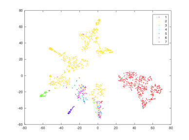
(a) Caltech7

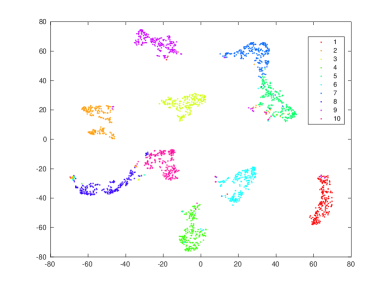
(b) Handwritten

Figure 1: Visualization of some clustering results.

Robustness Study

To examine the robustness of our method, we perform additional experiments by adding three commonly seen kinds of noise. We choose the famous MNIST database, which consists of gray-scale images of size $28\times 28$. There are 70000 samples in total. Since it is a single-view data, we construct a multi-view data set by adding different levels of noise to different views. Specifically, we first corrupt MNIST data by adding Gaussian noise with variance 0.01, 0.03, and 0.05; Salt&Pepper noise with density 0.05, 0.1, and 0.2; Speckle noise with variance 0.05, 0.1, and 0.15, respectively. Then, we concatenate them to form three three-view data sets. Some example images are shown in Figures 2-4. For these large data sets, we find that only SSCOMP and our method can handle it, while other recent multi-view clustering methods fail.

According to the results in Table 7, our method obtains better performance than SSCOMP in all metrics. This also verifies the advantage of multi-view learning which can exploit the complementarity of multi-view data. In terms of computation time, our method is 20 times faster than SSCOMP.

Table 7: Clustering performance on MNIST data.

Noise	Method	Acc	NMI	Purity	Time (s)
Gaussian	SSCOMP(1)	0.4300	0.4726	0.5965	1120.80
	SSCOMP(2)	0.4465	0.4749	0.5908	1151.50
	SSCOMP(3)	0.4418	0.4754	0.5920	1130.30
	LMVSC	0.5565	0.5096	0.6282	55.17
Speckle	SSCOMP(1)	0.4417	0.4770	0.5967	1314.90
	SSCOMP(2)	0.4560	0.4795	0.5995	1287.70
	SSCOMP(3)	0.4556	0.4855	0.6043	1303.40
	LMVSC	0.5920	0.5178	0.6183	66.01
Salt&Pepper	SSCOMP(1)	0.4536	0.4782	0.5964	1181.90
	SSCOMP(2)	0.4513	0.4822	0.6021	1306.10
	SSCOMP(3)	0.4816	0.4923	0.6307	1302.00
	LMVSC	0.5889	0.5374	0.6598	73.33

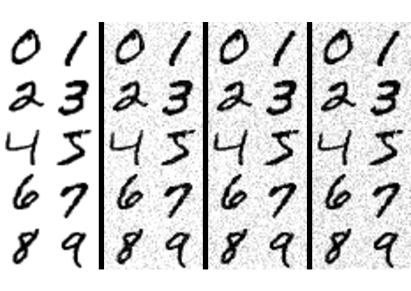
Figure 2: Some sample images of MNIST are shown in the 1st column. Corresponding noisy images contaminated by Gaussian noise with variance 0.01, 0.03, and 0.05, are displayed in the 2nd, 3rd, and 4th column, respectively.

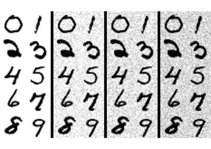
Figure 3: Some sample images of MNIST are shown in the 1st column. Corresponding noisy images contaminated by Speckle noise with variance 0.05, 0.1, and 0.15, are displayed in the 2nd, 3rd, and 4th column, respectively.

Parameter Analysis

During the experiments, we tune two parameters based on grid search, i.e., the number of anchors and $\alpha$. Taking Handwritten and MNIST data sets as examples, we show our model’s sensitivity to their values in Figures 5 and 6. We can see that $\alpha$ tends to have a small value since the performance is degraded when $\alpha$ increases. We have similar observation for anchor number. Too many anchors will make themselves less representative and introduce extra errors. Consequently, the performance will be deteriorated.

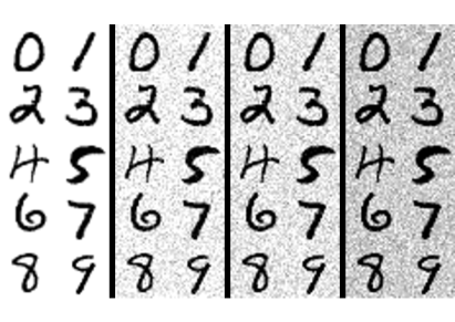
Figure 4: Some sample images of MNIST are shown in the 1st column. Corresponding noisy images contaminated by Salt&Pepper noise with density 0.05, 0.1, and 0.2, are displayed in the 2nd, 3rd, and 4th column, respectively.

Table 8: Description of single-view data sets.

Data Sets	#Feature	#Classes	#Sample
RCV1	1979	103	193844
CoverType	54	7	581012

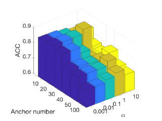
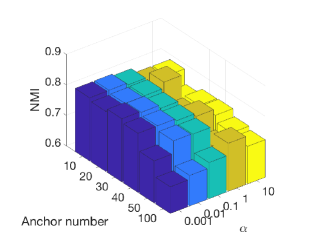
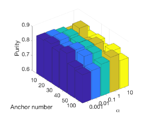
Figure 5: Sensitivity analysis of parameters for our method over Handwritten data set.

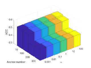
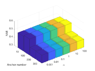
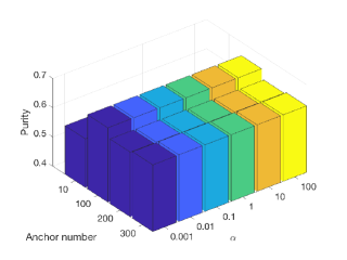
Figure 6: Sensitivity analysis of parameters for our method over MNIST data set.

Table 9: Results of single-view data sets.

Data Sets	Method	Acc	NMI	Purity	Time (s)
RCV1	KM	0.1846	0.2447	0.2550	1569.07
	LMVSC	0.1929	0.2600	0.2985	1035
CoverType	KM	0.2505	0.0617	0.3039	156.72
	LMVSC	0.3862	0.1273	0.4889	2755.8

Experiment on Single-View Data

We use two large-scale single-view data sets to demonstrate the performance of our algorithm on single-view data. Specifically, RCV1 consists of newswire stories from Reuters Ltd. CovType contains instances for predicting forest cover type from cartographic variables. Their statistics are summarized in Table 8. We found that SSCOMP can not finish within 24 hours, while many other large-scale subspace clustering (?; ?) methods run out of memory. For comparison, we include $k$-means (KM) as baseline. From Table 9, we can see that our method improves the performance significantly. Considering the size of data, our computation time is still reasonable. For CoverType, KM runs fast since the cluster number is quite small.

Conclusion

In this paper, we propose a novel multi-view subspace clustering algorithm. To the best of our knowledge, LMVSC is the very first effort of addressing the large-scale problem of multi-view subspace clustering. Our proposed method has a linear computation complexity, while maintaining high level of clustering accuracy. Specifically, for each view, one smaller graph is built between the raw data points and the generated anchors. Then, a novel integration mechanism is designed to merge those graphs, so that the eigen decomposition can be accelerated significantly. Furthermore, our proposed method also applies to single-view data. Extensive experiments on real data sets verify the effectiveness, efficiency, and robustness of the proposed method against other state-of-the-art techniques.

References

- [Affeldt, Labiod, and Nadif 2019] Affeldt, S.; Labiod, L.; and Nadif, M. 2019. Spectral clustering via ensemble deep autoencoder learning (sc-edae). arXiv preprint arXiv:1901.02291.
- [Brbić and Kopriva 2018] Brbić, M., and Kopriva, I. 2018. Multi-view low-rank sparse subspace clustering. Pattern Recognition 73:247–258.
- [Cao et al. 2015] Cao, X.; Zhang, C.; Fu, H.; Liu, S.; and Zhang, H. 2015. Diversity-induced multi-view subspace clustering. In CVPR, 586–594.
- [Chen and Cai 2011] Chen, X., and Cai, D. 2011. Large scale spectral clustering with landmark-based representation. In AAAI.
- [Elhamifar and Vidal 2013] Elhamifar, E., and Vidal, R. 2013. Sparse subspace clustering: Algorithm, theory, and applications. IEEE transactions on pattern analysis and machine intelligence 35(11):2765–2781.
- [Fan et al. 2018] Fan, J.; Tian, Z.; Zhao, M.; and Chow, T. W. 2018. Accelerated low-rank representation for subspace clustering and semi-supervised classification on large-scale data. Neural Networks 100:39–48.
- [Gao et al. 2015] Gao, H.; Nie, F.; Li, X.; and Huang, H. 2015. Multi-view subspace clustering. In ICCV, 4238–4246.
- [Han, Xiong, and Nie 2017] Han, J.; Xiong, K.; and Nie, F. 2017. Orthogonal and nonnegative graph reconstruction for large scale clustering. In IJCAI, 1809–1815.
- [Huang et al. 2019] Huang, W.; Yin, M.; Li, J.; and Xie, S. 2019. Deep clustering via weighted k-subspace network. IEEE Signal Processing Letters 26:1628–1632.
- [Kang et al. 2019a] Kang, Z.; Guo, Z.; Huang, S.; Wang, S.; Chen, W.; Su, Y.; and Xu, Z. 2019a. Multiple partitions aligned clustering. In IJCAI, 2701–2707.
- [Kang et al. 2019b] Kang, Z.; Pan, H.; Hoi, S. C.; and Xu, Z. 2019b. Robust graph learning from noisy data. IEEE Transactions on Cybernetics 1–11.
- [Kang et al. 2019c] Kang, Z.; Shi, G.; Huang, S.; Chen, W.; Pu, X.; Zhou, J. T.; and Xu, Z. 2019c. Multi-graph fusion for multi-view spectral clustering. Knowledge-Based Systems.
- [Kang et al. 2019d] Kang, Z.; Wen, L.; Chen, W.; and Xu, Z. 2019d. Low-rank kernel learning for graph-based clustering. Knowledge-Based Systems 163:510–517.
- [Kang et al. 2019e] Kang, Z.; Xu, H.; Wang, B.; Zhu, H.; and Xu, Z. 2019e. Clustering with similarity preserving. Neurocomputing 365:211–218.
- [Kang et al. 2020] Kang, Z.; Zhao, X.; Shi; Peng, c.; Zhu, H.; Zhou, J. T.; Peng, X.; Chen, W.; and Xu, Z. 2020. Partition level multiview subspace clustering. Neural Networks 122:279–288.
- [Kang, Peng, and Cheng 2015] Kang, Z.; Peng, C.; and Cheng, Q. 2015. Robust subspace clustering via smoothed rank approximation. IEEE Signal Processing Letters 22(11):2088–2092.
- [Li and Zhao 2017] Li, J., and Zhao, H. 2017. Large-scale subspace clustering by fast regression coding. In IJCAI.
- [Liu et al. 2013] Liu, G.; Lin, Z.; Yan, S.; Sun, J.; Yu, Y.; and Ma, Y. 2013. Robust recovery of subspace structures by low-rank representation. IEEE transactions on pattern analysis and machine intelligence 35(1):171–184.
- [Liu et al. 2019] Liu, X.; Zhu, X.; Li, M.; Wang, L.; Zhu, E.; Liu, T.; Kloft, M.; Shen, D.; Yin, J.; and Gao, W. 2019. Multiple kernel k-means with incomplete kernels. IEEE transactions on pattern analysis and machine intelligence.
- [Liu, He, and Chang 2010] Liu, W.; He, J.; and Chang, S.-F. 2010. Large graph construction for scalable semi-supervised learning. In ICML, 679–686.
- [Luo et al. 2018] Luo, S.; Zhang, C.; Zhang, W.; and Cao, X. 2018. Consistent and specific multi-view subspace clustering. In AAAI.
- [Ng, Jordan, and Weiss 2002] Ng, A. Y.; Jordan, M. I.; and Weiss, Y. 2002. On spectral clustering: Analysis and an algorithm. In NIPS, 849–856.
- [Nie et al. 2016] Nie, F.; Li, J.; Li, X.; et al. 2016. Parameter-free auto-weighted multiple graph learning: A framework for multiview clustering and semi-supervised classification. In IJCAI, 1881–1887.
- [Peng, Kang, and Cheng 2017] Peng, C.; Kang, Z.; and Cheng, Q. 2017. Subspace clustering via variance regularized ridge regression. In CVPR, 2931–2940.
- [Pourkamali-Anaraki and Becker 2018] Pourkamali-Anaraki, F., and Becker, S. 2018. Efficient solvers for sparse subspace clustering. arXiv preprint arXiv:1804.06291.
- [Shakhnarovich 2005] Shakhnarovich, G. 2005. Learning task-specific similarity. Ph.D. Dissertation, Massachusetts Institute of Technology.
- [Tang et al. 2019] Tang, C.; Zhu, X.; Liu, X.; and Wang, L. 2019. Cross-view local structure preserved diversity and consensus learning for multi-view unsupervised feature selection. In Proceedings of the AAAI Conference on Artificial Intelligence, volume 33, 5101–5108.
- [Wang et al. 2014] Wang, S.; Tu, B.; Xu, C.; and Zhang, Z. 2014. Exact subspace clustering in linear time. In AAAI.
- [Wang et al. 2016a] Wang, M.; Fu, W.; Hao, S.; Tao, D.; and Wu, X. 2016a. Scalable semi-supervised learning by efficient anchor graph regularization. IEEE Transactions on Knowledge and Data Engineering 28(7):1864–1877.
- [Wang et al. 2016b] Wang, Y.; Zhang, W.; Wu, L.; Lin, X.; Fang, M.; and Pan, S. 2016b. Iterative views agreement: an iterative low-rank based structured optimization method to multi-view spectral clustering. In IJCAI, 2153–2159. AAAI Press.
- [Wang et al. 2019] Wang, X.; Lei, Z.; Guo, X.; Zhang, C.; Shi, H.; and Li, S. Z. 2019. Multi-view subspace clustering with intactness-aware similarity. Pattern Recognition 88:50–63.
- [Xia et al. 2014] Xia, R.; Pan, Y.; Du, L.; and Yin, J. 2014. Robust multi-view spectral clustering via low-rank and sparse decomposition. In AAAI.
- [Xiao et al. 2015] Xiao, S.; Li, W.; Xu, D.; and Tao, D. 2015. Falrr: A fast low rank representation solver. In CVPR, 4612–4620.
- [Yao et al. 2019] Yao, S.; Yu, G.; Wang, J.; Domeniconi, C.; and Zhang, X. 2019. Multi-view multiple clustering. In IJCAI.
- [Ye and Tse 1989] Ye, Y., and Tse, E. 1989. An extension of karmarkar’s projective algorithm for convex quadratic programming. Mathematical programming 44(1-3):157–179.
- [Yin et al. 2018] Yin, M.; Gao, J.; Xie, S.; and Guo, Y. 2018. Multiview subspace clustering via tensorial t-product representation. IEEE Transactions on Neural Networks and Learning Systems 30(3):851–864.
- [You, Robinson, and Vidal 2016] You, C.; Robinson, D.; and Vidal, R. 2016. Scalable sparse subspace clustering by orthogonal matching pursuit. In CVPR, 3918–3927.
- [Zhan et al. 2018] Zhan, K.; Niu, C.; Chen, C.; Nie, F.; Zhang, C.; and Yang, Y. 2018. Graph structure fusion for multiview clustering. IEEE Transactions on Knowledge and Data Engineering.
- [Zhang et al. 2017] Zhang, C.; Hu, Q.; Fu, H.; Zhu, P.; and Cao, X. 2017. Latent multi-view subspace clustering. In CVPR, 4279–4287.