Josephson current between two $p$-wave superconducting nanowires in the presence of Rashba spin-orbit interaction and Zeeman magnetic fields

Abstract

Josephson current between two one-dimensional nanowires with proximity induced $p$-wave superconducting pairing is calculated in the presence of Rashba spin-orbit interaction, in-plane and normal magnetic fields. We show that Andreev retro-tunneling is realized by means of three channels. The main contribution to the Josephson current gives a scattering in a conventional particle-hole channel, when an electron-like quasiparticle reflects to a hole-like quasiparticle with opposite spin yielding a current which depends only on the order parameters’ phase differences $\varphi$ and oscillates with $4\pi$ period. Second anomalous particle-hole channel, corresponding to the Andreev reflection of an incident electron-like quasiparticle to an hole-like quasiparticle with the same spin orientation, survives only in the presence of the in-plane magnetic field. The contribution of this channel to the Josephson current oscillates with $4\pi$ period not only with $\varphi$ but also with orientational angle of the in-plane magnetic field $\theta$ resulting in a magneto-Josephson effect. Third anomalous particle-particle channel, which represents a reflection of an electron-like (hole-like) quasiparticle to a electron-like (hole-like) quasiparticle with opposite spin-orientation, oscillates only with the in-plane magnetic field orientation angle $\theta$. We present a detailed theoretical analysis of both DC and AC Josephson effects in such a system showing contributions from all these channels and discuss experiments which can test our theory.

I Introduction

A key model for realization of Majorana fermion (MF) in a condensed matter is a spinless $p$-wave superconductor (SC) kitaev01 ; kitaev03 . Majorana zero modes are excitations at zero energy which are typically localized at interface of the topological-non-topological phases and spatially separated from one another. They emerge as electrically neutral fermions indistinguishable from their antiparticles in subgap quasiparticle excitation spectrum of a topological superconductor (TSC). In $s$-wave superconductors, the quasiparticle excitations at the top of the supercoducting gap are indeed equal coherent superpositions of electrons and holes with opposite spins, and thus electrically neutral. Nevertheless, such a superposition of fermionic quasiparticles is not self-conjugate due to existence of spin. Therefore, MF can not appear in $s$-wave SC, and it is expected to occur in an effectively spinless $p$-wave SC kitaev01 . In $p$-wave SC model odd number of Majoranas reside at each end of the superconductor. However, electrons in conventional materials have spin-half particles; thus, the notion of a spinless SC does not seem immediately relevant to real physical systems.

Recently it was suggested that a topological (spinless $p$-wave) superconductivity can be effectively realized either in a spin-polarized normal metal or in a semiconductor nanowire with strong spin-orbit coupling under Zeeman magnetic field proximity-coupled to a conventional spin-singlet ($s$-wave) bulk SC lsd10 ; oro10 . Spin-orbit interactions split the energy spectrum shifting the energy branches along the momentum axis. In contrast, an in-plane Zeeman magnetic field shifts the energy of up- and down-spin electrons opening a gap in the spectrum at zero momentum. When the chemical potential is located in the gap the upper spin-subband becomes empty, and the system is transformed to an effectively “spinless” electron model. However, owing to the spin-orbit interactions-induced rotation of the spins at the opposite Fermi points, the proximity-induced $s$-wave interaction opens a pairing gap in the spectrum. The resulting state is closely related to a spinless $p$-wave superconductor. One of the virtues of this model is that the proximitized nanowire can be driven into a topological phase by tuning the magnetic field or the chemical potential (Fig. 1). The emergence of Majorana zero modes at a certain critical value of a control parameter is necessarily accompanied by the closing of the bulk gap kitaev01 , which corresponds to a topological quantum phase transition (that is, a quantum phase transition between topologically trivial and non-trivial states).

The topological phase in these wires is stable with respect to small perturbations (such as disorder) as long as they do not cause the bulk gap in the spectrum to collapse. The ability to realize the topological phase depends on the effective spin-orbit energy $E_{so}$, the proximity-induced gap $\Delta$ and the effective Zeeman energy $V_{Z}$ in the heterostructure. Note that highly controlled zero-energy quasi-particles Majoranas, produced in thin wire, can be utilized as a quantum information carrier qubit in quantum computer technology. MFs are exotic non-Abelian fermions obeying non-Abelian braiding statistics rg00 ; ivanov01 ; aoro11 . This unique property makes MF ideal for fault-tolerant quantum computation. These MFs typically arise at defect sites as Abrikosov vortex cores in bulk SCs, at interface of dielectric/TSC or normal metal/TSC, or at edges of TSC as localized excitations, and are topologically protected against any local perturbations. Essentially, two key points for the emergence of MFs are presented here: spin-orbit coupling (SOC) and superconducting proximity effect. A neutral excitation in a superconductor has a special property owing to the inherent particle-hole symmetry of the material: it is bound to zero energy, so that there is no cost to occupy such a state. One dimensional (1D) topological superconductor supports a non-local fermionic mode comprising two Majorana zero modes localized at opposite ends of the chain and are separated by a distance that can be much larger than the superconducting coherence length. An odd number of Majorana zero modes emerges per wire end; this is consistent with the fact that an even number of Majorana modes can pair up and locally form an Andreev state (which is a conventional fermionic state).

Recent investigations have shown gr01 ; ljl14 ; rm15 ; yw16 that a proximity of semiconductor with $s$-wave superconductor induces not only $s$-wave but also $p$-wave superconducting pairing in the semiconductor. The pairing symmetry of a BCS-type two dimensional (2D) superconductor without inversion symmetry when the twofold degeneracy of the electron energy spectrum is lifted by SOC has been studied gr01 ; edelstein89 ; faks04 to be a mixture of singlet and triplet symmetries. Recently Reeg and Maslov have shown rm15 by directly solving the fully quantum-mechanical Gor’kov equations that spin-triplet superconducting correlations are induced by Rashba SOC in both 1D and 2D proximity junctions via the proximity effect. Furthermore, the induced triplet component in 1D was shown to vanish when integrated over the momentum; this result is in agreement with Ref. [ljl14, ]. The induced triplet amplitude in 2D was found to have an odd-frequency component that is isotropic in momentum.

In this work we study Josephson junction ($JJ$) of two superconductors with $p$-wave pairing of spinfull electrons separated by a $\delta$-function like insulator potential. $JJ$ consisting of $p$-wave superconductors in both sides of the junction has been studied ksy04 for a $\delta$-like insulator potential in the absence of SOC and Zeeman magnetic field. Since the superconductor is in the topological phase, a fractional oscillation of Josephson current was obtained in Ref. [ksy04, ]. The emergence of Majorana zero mode results in exotic Josephson effects kitaev01 ; fk09 ; jpar11 ; jpar13 ; nats17 , when the current flowing between two topological superconductors in the junction oscillates with a fractional periodicity $4\pi$ instead of $2\pi$ periodicity in a conventional Josephson junction. Additionally, “spin Josephson current” nb04 ; asano06 ; brydon09 ; bat11 may flow across the junction, which is shown jpar11 ; jpar13 also to be $4\pi$ periodic in the field orientations as a manifestation of the Majorana modes.

Josephson current in a junction of two $s$-wave symmetric superconductors has been studied by us in our previous work nats17 . In this work we study the Josephson current through a junction of two superconductors with $p$-wave pairing of spinfull electrons. This problem has been usually studied for spinless model kitaev01 , although many aspects of spinfull $p$-wave symmetric $JJ$ have been investigated zclw12 ; kecs14 ; ehm16 ; bs19 ; mkc19 in the literatures. Furthermore, in this paper we want to understand how do SOC and external magnetic fields change Josephson current in p-type $JJ$ separated by a $\delta$-potential insulator. Similar effects have studied in Ref. [nats17, ] for a junction consisting of $s$-wave SCs separated by $\delta$-potential thin insulator. Note that, the Josephson current in the case of proximity induced both $s$- and $p$-wave pairings in $JJ$, as argued in several recent papers gr01 ; ljl14 ; rm15 ; yw16 , can be found by summing up a corresponding result of Ref. [nats17, ] with that presented in this paper. We show in this paper that the Andreev tunneling occurs in three channels, and clarify the origin of these channels. Two additional channels seem to vanish with in-plane magnetic field. All contributions to the Josphson current oscillate with fractional periodicity either with phase difference of the SC order parameters $\varphi$ or with tilded angle $\theta$ between the in-plane magnetic field and JJ. Simultaneous action of SOC and Zeeman magnetic fields results in openning of a forbidden gap in dependence of Josephson current on the phases at some definite values of SOC and magnetic fields.

The paper is organized as follow. In the next Section formulation of the problem is presented. In Section III Andreev bound state energy is calculated for different values of the external parameters as SOC constant, Zeenam energies for the magnetic fields normal to the junction $h$ and the tilted magnetic field ${\bf B}$ lying in the junction plane and forming an angle $\theta$ with SC wire. Section IV describes Josephson current as well as magneto-Josephson effect in the junction. $ac$-Josephson current and effects of SOC and magnetic field on the Shapiro step in the $JJ$ of p-wave superconductors are studied in the last Section V.

II Model and formulation of the problem

We consider a junction of two $1D$ nanowires of proximity induced $p_{x}$-wave pairing symmetry superconductivity, having the effective pairing potentials $\Delta_{L}$ and $\Delta_{R}$ on the left(L)- and right (R)-side of an insulating potential barrier separated two superconductors, in the presence of Rashba spin-orbital interaction and external Zeeman magnetic fields. Hamiltonian for such a system reads

$$\hat{H}=\hat{H}_{SC}+\hat{H}_{R},$$ (1)

where $\hat{H}_{SC}$ is Hamiltonian of the nanowire in the presence of external magnetic fields and $\hat{H}_{R}$ represents Rashba SOI. The former term is given by

$$\hat{H}_{SC} = \int dx\Bigg{\{}\sum_{\sigma,\sigma^{\prime}}\psi_{\sigma}^{{\dagger}}(x)\Big{[}[\xi_{\hat{k}}+U(x)]\sigma_{0}+h\sigma_{z}$$ (2)

$$+B\{[\sigma_{x}\cos\theta_{1}+\sigma_{y}\sin\theta_{1}]\theta(-x)+[\sigma_{x}\cos\theta_{2}$$

$$+\sigma_{y}\sin\theta_{2}]\theta(x)\}\Big{]}\psi_{\sigma^{\prime}}(x)$$

$$+\left[\Delta_{L}\theta(-x)+\Delta_{R}\theta(x)\right]\psi_{\uparrow}^{{\dagger}}(x)\psi_{\downarrow}^{{\dagger}}(x)+{\rm h.c.}\Bigg{\}},$$

where $\xi_{\hat{k}}=\epsilon\left(\frac{\hbar}{i}\frac{\partial}{\partial x}\right)-\epsilon_{F}$ denotes the electron kinetic energy as measured from the Fermi level $\epsilon_{F}$, $\psi_{\sigma}(x)$ is the electron annihilation operator, $h$ and ${\bf B}$ are external Zeeman magnetic fields in $z$ direction and in the x-y plane respectively, $\theta(x)$ is the Heaviside step function, and $\sigma_{x,y,z}$ and $\sigma_{0}$ denote Pauli and identity matrices respectively in spin space. Note that the magnetic field ${\bf B}$ forms an angle $\theta$ with wire which can be tuned externally. In what follows, we choose ${\bf B}$ in the left side of the junction to be aligned along the wire ($\theta_{L}=0$) while in the right side it is chosen to make an angle $\theta$ with it ($\theta_{R}=\theta$). In Eq. (2), the pairing potential $\Delta_{R}$ in the right of the junction is chosen to have a phase difference $\varphi$ compared to its left counterpart: $\Delta_{R}=|\Delta|\exp(i\varphi)$ and $\Delta_{L}=|\Delta|$. The potential $U(x)=U_{0}\delta(x)$, located at $x=0$, represents the barrier potential between two superconductors. The Hamiltonian of Rashba SOI can be written as

$$\hat{H}_{R}=\sum_{\sigma,\sigma^{\prime}}\int dx\psi_{\sigma}^{{\dagger}}(x)\alpha\left[v_{x}\sigma_{z}\right]\psi_{\sigma^{\prime}}(x),$$ (3)

where $\alpha$ is the strength of Rashba SOI which is chosen to be the same for both wires.

The order parameter $\Delta_{\alpha,\beta}^{t}(\hat{\bf k})$ for triplet pairing with $S=1$ can be presented as leggett75 ; ms98

$$\Delta_{\alpha,\beta}^{t}(\hat{\bf k})=\Delta{\bf d}({\bf k})(i{\bf\sigma}\sigma_{y})_{\alpha,\beta}$$ (4)

where ${\bf d}({\bf k})$ is odd function of ${\bf k}$, ${\bf d}({\bf k})=-{\bf d}(-{\bf k})$, and can be expanded over spherical harmonics

$$d_{\alpha}({\bf k})=\sum_{m=-l}^{l}b_{l,m}^{\alpha}Y_{l,m}(\hat{\bf k}).$$ (5)

The quantum number $l$ in Eq. (5) takes odd values $1,3,\dots$ corresponding to states of $p,f,\dots$- pairings. The coefficient $b_{l,m}^{\alpha}$ can be identified as $\alpha$ component of the superconducting order parameter with given $l$ and $m$. For a simple case of $p$-wave pairing for $l=1$ and $m=-1,0,1,$ $d_{\alpha}({\bf k})$ can be expressed with the appropriate expressions for the spherical harmonics $Y_{1,-1}\propto(\hat{k}_{x}-i\hat{k}_{y})$, $Y_{1,0}\propto\hat{k}_{z}$, and $Y_{1,1}\propto(\hat{k}_{x}+i\hat{k}_{y})$, as,

$$d_{\alpha}({\bf k})=A_{\alpha,i}\hat{k}_{i}.$$ (6)

Thereby, the $p_{x}$-wave symmetric order parameter $\Delta_{a,\sigma}(x,k_{x})$ on the $a=R,L$-side of a junction between two superconductors aligned along the $x$-axis can be expressed as,

$$\Delta_{a,\sigma}(x,k_{x})=\Delta_{a}\frac{k_{x}}{k_{F}}.$$ (7)

It is advantageous to use a four component field operator for bulk superconductor at the right ($a=R$) and left ($a=L$) side of the junction as,

$$\Psi^{{\dagger}}_{a}(x)=\left(\psi_{a,\uparrow,+}^{{\dagger}}(x),\psi_{a,\downarrow,+}^{{\dagger}}(x),\psi_{a,\downarrow,-}(x),\psi_{a,\uparrow,-}(x)\right)$$ (8)

Here the third subscript of the annihilation operator (which we shall designate henceforth as $b$) labels the right- ($b=+$) and the left-moving $(b=-$) quasiparticles respectively while the index $a=R,L$ denotes either right ($R=-$) or left ($L=+$) superconductor. In terms of the field operator given by Eq. (8), the Hamiltonian (Eq. (1)) can be written as $\hat{H}=\sum_{a=R,L}\int dx\Psi^{{\dagger}}_{a}(x)\mathcal{H}_{a}\Psi_{a}(x)$ using the Pauli matrices $\sigma_{i}$ in spin- and $\tau_{i}$ in particle-hole spaces. From Eqs. (1) and (2), we find

$$\mathcal{H}_{R}=\xi_{k,b}\tau_{z}\sigma_{0}+h\tau_{0}\sigma_{z}-ik\alpha\tau_{z}\sigma_{z}$$ (9)

$$+B\tau_{z}\left(\sigma_{x}\cos\theta+\sigma_{y}\sin\theta\right)+|\Delta|(\tau_{x}\cos\varphi-\tau_{y}\sin\varphi)\sigma_{z},$$

and ${\mathcal{H}}_{L}={\mathcal{H}}_{R}(\theta=0;\varphi=0)$. In Eq. (9), the energy spectrum of the electrons are linearized around the positive and negative Fermi momenta leading to $\xi_{k,b}=bv_{F}\left(-i\frac{\partial}{\partial x}-k_{F}\right)$, where $v_{F}$ is the Fermi energy. Note that the Hamiltonian $\mathcal{H}_{R,L}$ acquires a magnetism-superconductivity duality nab08 ; jpar13 in the absence of the kinetic term, implying that it becomes invariant under the transformation $\{\Delta,\epsilon_{F},\varphi,\tau_{i}\}\to\{B,h,-\theta,\sigma_{i}\}$. The existence of a magneto-Josephson effect in a topological insulator is known to be a result of this duality jpar13 . We shall see that for the system we study, the magneto-Josephson effect takes place even in the presence of the additional quadratic kinetic energy term of the electrons.

The energy spectrum of a quasi-particle in a ’bulk’ quasi-1D superconductor is determined from the expression ${\rm Det}|\mathcal{H}_{R}-E|=0$, yielding

$$\left(E^{2}-v_{F}^{2}k^{2}+\alpha^{2}k^{2}-h^{2}-B^{2}-|\Delta|^{2}\right)^{2}+4\left(Ekv_{F}+h\alpha k\right)^{2}-4|\Delta|^{2}\left(v_{F}^{2}k^{2}+B^{2}+h^{2}\right)=0.$$ (10)

This equation does not yield a simple analytic expression for $E$, while it contains a linear in energy term, which is a result of an alignment of ${\bf h}$ and the effective magnetic field of the SOI $\propto\alpha k$. The linear in $E$ term vanishes for either $h=0$ or $\alpha=0$, and Eq. (10) turns to quadratic equation for $E^{2}$, which gives two symmetric dispersion branches for quasi-particles and quasi-holes. Note that square of the momentum $k^{2}_{\pm}$, where the subscripts indices indicate the spin branches, can be obtained from Eq. (10). The evident expression for $k^{2}_{\pm}$ is presented by Eq. (75) in Appendix. Equation (10) is strongly simplified for different limiting cases, and yields the following expressions for the energy dispersion,

$$E=\begin{cases}\pm\sqrt{|\Delta|^{2}-v_{F}^{2}k^{2}}&\text{if}\qquad\alpha=B=h=0,\\ s\left[\sqrt{|\Delta|^{2}-v_{F}^{2}k^{2}}\pm\sqrt{B^{2}+h^{2}}\right]&\text{if}\qquad\alpha=0,B\neq 0,h\neq 0,\\ s\sqrt{B^{2}+|\Delta|^{2}-(v_{F}^{2}+\alpha^{2})k^{2}\pm 2\sqrt{v_{F}^{2}\alpha^{2}k^{4}+|\Delta|^{2}B^{2}-v_{F}^{2}k^{2}B^{2}}}&\text{if}\qquad h=0,\alpha\neq 0,B\neq 0,\end{cases}$$ (11)

where $s=\pm$ indicates the particle- and hole-branches of the spectrum. The energy levels of the Bogolyubov-de Gennes (BdG) quasi-particles lie in the gap, symmetric to the Fermi level. SOI and/or magnetic field $h$ split both electron and hole levels due to Rashba ’momentum-shifting’ and/or Zeeman effect. The ’Fermi points’ around $+k_{F}$ and $-k_{F}$ are split also due to these effects. At the same time, the magnetic field makes the energy dispersion asymmetric. Note that in our case, all energies are measured from the Fermi energy; thus the condition for realization of a topological non-trivial superconducting gapped phase is $|\Delta|^{2}\geq B^{2}+h^{2}$, jpar13 . Indeed, zero energy mode ($E=0$) at the center of the Brillouin zone ($k=0$) appears according to Eq. (10) under the condition $|\Delta|^{2}-B^{2}-h^{2}=0$.

BdG equations for an isolated ’bulk’ superconductor in the case of an infinitely high potential between the right (R)- and left (L) parts ($a=R,L$) of the barrier is written as

$$\mathcal{H}_{a}\mathbf{\eta}_{a}(x)=E\mathbf{\eta}_{a}(x),\quad a=R,L$$ (12)

where the four-component vector $\eta_{a}(x)=\left(\eta_{a,\uparrow,+}^{{\dagger}}(x),\eta_{a,\downarrow,+}^{{\dagger}}(x),\eta_{a,\downarrow,-}(x),\eta_{a,\uparrow,-}(x)\right)$ denotes the BdG wave function. In order to get the explicit expressions for the wave functions $\eta_{a,\sigma,b}$ and $\eta_{a,{\bar{\sigma}},b}^{\ast}$ we write Eq. (12) for finite value of the external parameters ${\bf B}$, $h$ and $\alpha$ as

$$(E+iabv_{F}k+iab\alpha k-h)\eta_{a,\uparrow,b}-Be^{-i\theta}\eta_{a,\downarrow,b}$$

$$-\Delta_{a}\eta^{\ast}_{a,\downarrow,\bar{b}}=0$$ (13)

$$(E+iabv_{F}k-iab\alpha k+h)\eta_{a,\downarrow,b}-Be^{i\theta}\eta_{a,\uparrow,b}$$

$$+\Delta_{a}\eta^{\ast}_{a,\uparrow,\bar{b}}=0$$ (14)

$$(E-iabv_{F}k-iab\alpha k-h)\eta^{\ast}_{a,\downarrow,\bar{b}}+Be^{-i\theta}\eta^{\ast}_{a,\uparrow,\bar{b}}$$

$$-\Delta_{a}^{\ast}\eta_{a,\uparrow,b}=0$$ (15)

$$(E-iabv_{F}k+iab\alpha k+h)\eta^{\ast}_{a,\uparrow,\bar{b}}+Be^{i\theta}\eta^{\ast}_{a,\downarrow,\bar{b}}$$

$$+\Delta_{a}^{\ast}\eta_{a,\downarrow,b}=0.$$ (16)

In order to understand the features of Eqs. (13)-(16) one considers several asymptotic cases. In the absence of the in-plane magnetic field ${\bf B}=0$, these equations link a particle wave function $\eta_{a,\sigma,b}$ with the hole one $\eta^{\ast}_{a,\bar{\sigma},\bar{b}}$ of an opposite spin-polarized and opposite direction-moved quasiparticle state ksy04 and vice-versa, provided that the system is in a superconducting phase, $\Delta_{a}\neq 0$. Instead, in the absence of a superconducting phase, $\Delta_{a}=0$, these equations link a particle (hole) wave function $\eta_{a,\sigma,b}$ with the particle (hole) wave function with opposite spin-polarized quasiparticle state $\eta_{a,\bar{\sigma},b}$ moving in the same direction provided that ${\bf B}\neq 0$. However, in the presence of in-plane magnetic field ${\bf B}\neq 0$ in the superconduction phase $\Delta_{a}\neq 0$, Eqs. (13)-(16) connect a particle wave function $\eta_{a,\sigma,b}$ (a hole wave function $\eta^{\ast}_{a,\sigma,\bar{b}}$) with hole (particle) wave functions with the same $\eta^{\ast}_{a,\sigma,\bar{b}}$ ( $\eta_{a,\sigma,b}$) and opposite $\eta^{\ast}_{a,\bar{\sigma},\bar{b}}$ ( $\eta_{a,\bar{\sigma},b}$) spin-polarized quasiparticle states moving in the direction opposite to the particle (hole) one. Eqs. (13)-(16) allow us to calculate all possible ratios $\eta^{\ast}_{a,\sigma,b}/\eta_{a,{\bar{\sigma}},{\bar{b}}}$, $\eta^{\ast}_{a,\sigma,b}/\eta_{a,\sigma,{\bar{b}}}$, and $\eta_{a,\sigma,b}/\eta_{a,{\bar{\sigma}},b}$, $\eta^{\ast}_{a,\sigma,b}/\eta^{\ast}_{a,{\bar{\sigma}},b}$. Furthermore, we note that only the ratio $\eta^{\ast}_{a,\sigma,b}/\eta_{a,{\bar{\sigma}},{\bar{b}}}$ is non-zero for ${\bf B}=0$, which corresponds to the conventional Andreev reflection at the boundary of a superconductor with normal metal or insulator ksy04 . Eqs. (13)-(16) provide the following expressions for these ratios for arbitrary values of the parameters $\alpha$, ${\bf B}$, $h$,

$$\frac{\eta^{\ast}_{a,\uparrow,{\bar{b}}}}{\eta_{a,\downarrow,b}}=-\frac{1}{\Delta_{a,b}}\Bigg{\{}E+iabkv_{F}-iab\alpha k+h-$$

$$\frac{2B^{2}(E-iab\alpha k)}{(E-h)^{2}+(kv_{F}+\alpha k)^{2}+B^{2}-\Delta_{a,b}^{2}}\Bigg{\}}$$ (17)

$$\frac{\eta^{\ast}_{a,\uparrow,{\bar{b}}}}{\eta_{a,\uparrow,b}}=\frac{Be^{i\theta}}{\Delta_{a,b}}\Bigg{\{}1-$$

$$\frac{2(E+iab\alpha k)(E+iabkv_{F}-iab\alpha k+h)}{(E+h)^{2}+(kv_{F}-\alpha k)^{2}+B^{2}-\Delta_{a,b}^{2}}\Bigg{\}},$$ (18)

$$\frac{\eta_{a,\uparrow,b}}{\eta_{a,\downarrow,b}}=\frac{2B(E-iab\alpha k)e^{-i\theta}}{(E-h)^{2}+(kv_{F}+k\alpha)^{2}+B^{2}-\Delta_{a,b}^{2}};$$ (19)

where $\Delta_{a,b}=b\Delta_{a}$ according to Eq. (7), and $\Delta_{R}=|\Delta|\exp(i\varphi)$ and $\Delta_{L}=|\Delta|$. Note that the expressions for $\frac{\eta^{\ast}_{a,\downarrow,{\bar{b}}}}{\eta_{a,\uparrow,b}}$, $\frac{\eta^{\ast}_{a,\downarrow,{\bar{b}}}}{\eta_{a,\downarrow,b}}$, and $\frac{\eta_{a,\downarrow,b}}{\eta_{a,\uparrow,b}}$ can be obtained respectively from Eqs. (17), (18), and (19) by replacing $\theta\to-\theta$, $\alpha\to-\alpha$, $h\to-h$, and by reversing the total sign of these expressions. According to these expressions the reflection channels, determined by the ratios $\frac{\eta^{\ast}_{a,\downarrow,{\bar{b}}}}{\eta_{a,\downarrow,b}}$, and $\frac{\eta_{a,\downarrow,b}}{\eta_{a,\uparrow,b}}$, vanish with in-plane magnetic field ${\bf B}$.

We note from Eqs. (13)-(16) that the dependencies of these equations on $\varphi$ and $\theta$ are completely removed by transforming the wave functions as

$$\eta^{\ast}_{a}(x) \to \left(e^{-i(\varphi-\theta)/2}\eta_{a,\uparrow,\bar{b}}^{\ast}(x),~{}e^{-i(\varphi+\theta/2)}\eta_{a,\downarrow,\bar{b}}^{\ast}(x),\right.$$ (20)

$$\left.~{}e^{i(\varphi+\theta)/2}\eta_{a,\downarrow,b}(x),~{}e^{i(\varphi-\theta)/2}\eta_{a,\uparrow,b}(x)\right).$$

In the transformed basis one has

$$\frac{\eta^{\ast}_{a,\uparrow,b}}{\eta_{a,\uparrow,{\bar{b}}}}\to e^{-i(\varphi-\theta)}\frac{\eta^{\ast}_{a,\uparrow,b}}{\eta_{a,\uparrow,{\bar{b}}}},\quad\frac{\eta^{\ast}_{a,\downarrow,b}}{\eta_{a,\downarrow,{\bar{b}}}}\to e^{-i(\varphi+\theta)}\frac{\eta^{\ast}_{a,\downarrow,b}}{\eta_{a,\downarrow,{\bar{b}}}}$$ (21)

$$\frac{\eta^{\ast}_{a,\uparrow,b}}{\eta_{a,\downarrow,{\bar{b}}}}\to e^{-i\varphi}\frac{\eta^{\ast}_{a,\uparrow,b}}{\eta_{a,\downarrow,{\bar{b}}}},\quad\frac{\eta^{\ast}_{a,\downarrow,b}}{\eta_{a,\uparrow,{\bar{b}}}}\to e^{-i\varphi}\frac{\eta^{\ast}_{a,\downarrow,b}}{\eta_{a,\uparrow,{\bar{b}}}}$$ (22)

$$\frac{\eta^{\ast}_{a,\uparrow,b}}{\eta_{a,\downarrow,b}^{\ast}}\to e^{i\theta}\frac{\eta^{\ast}_{a,\uparrow,b}}{\eta_{a,\downarrow,b}^{\ast}},\quad\frac{\eta_{a,\uparrow,b}}{\eta_{a,\downarrow,b}}\to e^{-i\theta}\frac{\eta_{a,\uparrow,b}}{\eta_{a,\downarrow,b}}.$$ (23)

The different ratios that appear in the left hand-side of Eqs. (21)-(23) can be understood on follows. The ratio $\eta^{\ast}_{a,\sigma,b}/\eta_{a,{\bar{\sigma}},{\bar{b}}}$ corresponds to the amplitude of conventional Andreev reflection channel which constitutes reflection of an electron-like quasiparticle to a hole-like quasiparticle with opposite spin on a N-S interface. In contrast, the ratio $\eta^{\ast}_{a,\sigma,b}/\eta_{a,\sigma,{\bar{b}}}$ which is finite only in the presence of SOC and/or magnetic field, represents amplitude of Andreev reflection channel where the electron-like quasiparticle incident on the interface is reflected to a hole-like quasiparticle state with the same spin orientation. Finally, the ratio $\eta_{a,\sigma,b}/\eta_{a,{\bar{\sigma}},b}$ represents a usual reflection channel of an electron-like quasiparticle on the boundary without creation of a Cooper pair in a superconducting part of the junction. We note that the ratio of wave functions in Eq. (21) depend on both $\varphi$ and $\theta$ while those in Eqs. (22) and (23) depend on either $\varphi$ or $\theta$. This suggests that the ratios (21) and (22) are responsible for the dependence of observable parameters on the order parameter phase difference $\varphi$, whereas the ratios (21) and (23) are responsible for the dependence on the magnetic field orientation angle $\theta$.

Figure 1: (a) Splitting of an electron’s energy spectrum in the presence of Rashba spin-orbital interaction is depicted by dashed curve. Zeeman magnetic field removes the degeneracy at the cross-point of two spin- polarized spectra, and opens a gap of $2E_{z}$ width; (b) the band structure of 1D semiconductor with strong spin- orbit interaction, transformed to a superconducting state due to proximity effect.

In what follows, we shall look for the localized subgap Andreev bound states with $\epsilon(k)<|\Delta|$ for the Josephson junction of two nanowires described by Eq. (1).

III Andreev bound states, Josephson and magneto-Josephson effects

In order to obtain a solution for the Andreev bound states for the junction described by Eq. (2) one follows the method used in Ref. [ksy04, ]. The energy spectrum of an electron is splitted in the presence of Rashba SOC and/or Zeeman magnetic field, so that the Fermi level crosses the dispersion curve at four points, corresponding to right-mover $k_{F+}$, $k_{F-}$ and left-mover $-k_{F+}$, $-k_{F-}$ particles with oppositely polarized spin-states (see, Fig. 1), and $k_{F+}-k_{F-}\to 0$, $k_{F+},k_{F-}\to k_{F}$ as $\alpha,B,h\to 0$. Furthermore, a condensation of the electron pairs in a superconducting state opens a gap around the Fermi level as is shown in Fig.1b. We neglect here a difference between $k_{F}$ and $k_{F+}$, $k_{F-}$, and take $k_{F+}\approx k_{F-}\equiv k_{F}$. We assume that a transition occurs between the states with the same chirality. In order to obtain the wave function for $L$ and $R$ superconductors we superpose the wave functions for the left ($-$) and right ($+$) moving BdG quasiparticles correspondingly around the Fermi levels $k_{F}$, and $-k_{F}$ with arbitrary coefficients,

$$\mathbf{\eta}_{a}(x)=e^{{\rm sgn}(a)kx}\left\{e^{ik_{F}x}A_{a}\left(\begin{array}[]{ccc}\eta_{a,\uparrow,+}(k)\\ \eta_{a,\downarrow,-}(k)\\ \eta_{a,\downarrow,-}^{\ast}(k)\\ \eta_{a,\uparrow,+}^{\ast}(k)\end{array}\right)+e^{-ik_{F}x}B_{a}\left(\begin{array}[]{ccc}\eta_{a,\uparrow,-}(k)\\ \eta_{a,\downarrow,+}(k)\\ \eta_{a,\downarrow,+}^{\ast}(k)\\ \eta_{a,\uparrow,-}^{\ast}(k)\end{array}\right)\right\}$$ (32)

where ${\rm sgn}(a)=+(-)$ for $a=L(R)$. SOC and magnetic field remove the spin degeneracy in a quasi-particle ($\eta_{a,b}$) and a quasi-hole ($\eta^{\ast}_{a,b}$) wave functions, and thereby split the wave functions written for the conventional superconductors ksy04 as is shown in the above given expression.

Andreev bound state energies are obtained by imposing the usual boundary conditions on each component of these wave functions $\eta_{a}(x)$. For a barrier modeled by the delta function potential $U(x)=U_{0}\delta(x)$, the boundary conditions are provided at the merging point $x=0$ of two superconductors as,

$$\mathbf{\eta}_{L}(0)=\mathbf{\eta}_{R}(0),\qquad\qquad\partial_{x}\mathbf{\eta}_{R}-\partial_{x}\mathbf{\eta}_{L}=k_{F}Z\mathbf{\eta}(0),$$ (33)

where $Z=2mU_{0}/\hbar^{2}k_{F}$ and the transmission coefficient $D$ is expressed through $Z$ as $D=4/(Z^{2}+4)$.

By choosing a pair of the wave functions from Eq. (32) and substituting they into the boundary conditions (33) one gets four linear homogeneous equations. The energy of the Andreev bound state for a transmission of the barrier through a particular channel is obtained from the determinant of these linear homogeneous equations. Selection, e.g. the second and fourth equations of the wave function (32) under the boundary conditions (33) yields the following expression for the determinant,

$${\tilde{F}}_{\uparrow\downarrow}^{\ast}=\frac{1}{D}\eta_{+,\downarrow,+}\eta_{-,\downarrow,-}\eta_{+,\downarrow,-}\eta_{-,\downarrow,+}F^{\ast}_{\uparrow\downarrow},$$ (34)

where

$$F_{\uparrow\downarrow}^{\ast}=\left[\frac{\eta^{\ast}_{-,\uparrow,-}}{\eta_{-,\downarrow,+}}-\frac{\eta^{\ast}_{+,\uparrow,-}}{\eta_{+,\downarrow,+}}\right]\left[\frac{\eta^{\ast}_{+,\uparrow,+}}{\eta_{+,\downarrow,-}}-\frac{\eta^{\ast}_{-,\uparrow,+}}{\eta_{-,\downarrow,-}}\right]-$$

$$(1-D)\left[\frac{\eta^{\ast}_{+,\uparrow,-}}{\eta_{+,\downarrow,+}}-\frac{\eta^{\ast}_{-,\uparrow,+}}{\eta_{-,\downarrow,-}}\right]\left[\frac{\eta^{\ast}_{-,\uparrow,-}}{\eta_{-,\downarrow,+}}-\frac{\eta^{\ast}_{+,\uparrow,+}}{\eta_{+,\downarrow,-}}\right].$$ (35)

Using Eq. (17) in this expression one gets an explicit expression for $F_{\uparrow\downarrow}^{\ast}$

$$F_{\uparrow\downarrow}^{\ast}=-\frac{4e^{-i\varphi}}{|\Delta|^{2}M^{2}_{-}}\Bigg{\{}\left[(E+h)M_{-}+2B^{2}E\right]^{2}-D\cos^{2}\frac{\varphi}{2}\times$$

$$\left[\left[(E+h)M_{-}-2B^{2}E\right]^{2}+\left[k(v_{F}-\alpha)M_{-}+2B^{2}\alpha k\right]^{2}\right]\Bigg{\}},$$ (36)

where

$$M_{\pm}=(E\pm h)^{2}+(v_{F}\mp\alpha)^{2}k^{2}+B^{2}-|\Delta|^{2}.$$ (37)

The expression for $F_{\downarrow\uparrow}^{\ast}$ is obtained from Eq. (36) by replacing $\alpha\to-\alpha$, $h\to-h$ and $M_{-}\to M_{+}$, where $M_{+}(\alpha,h,B,\Delta)=M_{-}(-\alpha,-h,B,\Delta)$. Solution of the equation $F_{\uparrow\downarrow}^{\ast}(E_{\uparrow\downarrow})=0$ for energy, where $F_{\uparrow\downarrow}^{\ast}$ is given by Eq. (36), yields a contribution to the Andreev overlap energy $E_{\uparrow\downarrow}$ in the particle-hole channel.

Now we choose other pair, the first and fourth wave functions of (32), and substitute they into the boundary conditions (33). The determinant of four linear homogeneous equations yields the following expression to find the Andreev quasi-particle energy in the anomalous particle-hole channel, where the transition occurs between the spin states with the same chirality,

$${\tilde{F}}_{\sigma\sigma}^{\ast}(k)=\frac{1}{D}\eta_{+,\sigma,+}(k)\eta_{-,\sigma,-}(k)\eta_{+,\sigma,-}(k)\eta_{-,\sigma,+}(k)F^{\ast}_{\sigma\sigma}(k),$$ (38)

where $F^{\ast}_{\uparrow\uparrow}(k)$ ($F^{\ast}_{\downarrow\downarrow}(k)$) is obtained from Eq. (35) by replacing all spin-down (all spin-up) with spin-up (spin-down). The evident expression for $F^{\ast}_{\uparrow\uparrow}(k)$ is obtained by using the ratio (18), which reads as,

$$F_{\uparrow\uparrow}^{\ast}=\frac{16B^{2}e^{-i(\phi-\theta)}}{|\Delta|^{2}M^{2}_{+}}\Bigg{\{}\left(Ekv_{F}+\alpha hk\right)^{2}-$$

$$|\Delta|^{2}\left(E^{2}+\alpha^{2}k^{2}\right)\left[1-D\cos^{2}\frac{(\phi-\theta)}{2}\right]\Bigg{\}}.$$ (39)

The expression for $F^{\ast}_{\downarrow\downarrow}(k)$ can be obtained from Eq. (39) by replacing $\alpha\to-\alpha$, $h\to-h$, $\theta\to-\theta$, and $M_{+}\to M_{-}$. The general feature of the Andreev quasi-particle energy in the anomalous particle-hole channel $E_{\uparrow\uparrow}$ with the same spin orientation is that it takes non-zero values only in the presence of in-plane magnetic field ${\bf B}$. Therefore, it depends on the angle $\theta$ between the junction and in-plane magnetic field. Oscillation of the Josephson current with $\theta$ yields a fractional magneto-Josephson effect.

Choice of the first and second equations of the wave function (32) under the boundary conditions (33) yields the following expression to determine the Andreev bound state energy in the anomalous particle-particle or hole-hole channel,

$${\tilde{F}}_{\uparrow\downarrow}(k)=\frac{1}{D}\eta_{-,\downarrow,-}(k)\eta_{+,\downarrow,+}(k)\eta_{+,\downarrow,-}(k)\eta_{-,\downarrow,+}(k)F_{\uparrow\downarrow}(k),$$ (40)

where $F_{\uparrow\downarrow}(k)$ is written as

$$F_{\uparrow\downarrow}=\left[\frac{\eta_{+,\uparrow,+}}{\eta_{+,\downarrow,+}}-\frac{\eta_{-,\uparrow,+}}{\eta_{-,\downarrow,+}}\right]\left[\frac{\eta_{-,\uparrow,-}}{\eta_{-,\downarrow,-}}-\frac{\eta_{+,\uparrow,-}}{\eta_{+,\downarrow,-}}\right]-$$

$$(1-D)\left[\frac{\eta_{+,\uparrow,+}}{\eta_{+,\downarrow,+}}-\frac{\eta_{-,\uparrow,-}}{\eta_{-,\downarrow,-}}\right]\left[\frac{\eta_{-,\uparrow,+}}{\eta_{-,\downarrow,+}}-\frac{\eta_{+,\uparrow,-}}{\eta_{+,\downarrow,-}}\right].$$ (41)

The evident expression for $F_{\uparrow\downarrow}$ can be obtained by substituting Eq. (19) into Eq. (41), which yields,

$$F_{\uparrow\downarrow}=-\frac{16B^{2}e^{-i\theta}}{M^{2}_{-}}\Big{\{}\alpha^{2}k^{2}-\left(E^{2}+\alpha^{2}k^{2}\right)D\sin^{2}\frac{\theta}{2}\Big{\}}.$$ (42)

Note that the expression for $F_{\downarrow\uparrow}(k)$ can be obtained from Eq. (41) by replacing $\alpha\to-\alpha$, $h\to-h$, $\theta\to-\theta$, and $M_{-}\to M_{+}$. The main feature of the Andreev bound state energy in the anomalous particle-particle channel is that it survives only in the presence of the in-plane magnetic field ${\bf B}$ and the spin-orbit interaction $\alpha$. $E^{\prime}_{\uparrow\downarrow}$ and $E^{\prime}_{\downarrow\uparrow}$ vanish in the absence of one of the factors either ${\bf B}$ or $\alpha$, and they depend on the angle $\theta$ between the in-plane magnetic field orientation and the junction, contributing to the fractional magneto-Josephson effect.

Andreev bound state energies and Josephson current, corresponding to different tunneling channels, demonstrate completely different oscillation. The conditions $F_{\uparrow\downarrow}^{\ast}(E_{\uparrow\downarrow})=0$ and $F_{\downarrow\uparrow}^{\ast}(E_{\downarrow\uparrow})=0$ with Eq. (36) for $F_{\uparrow\downarrow}^{\ast}(E)$ provide contributions to the Andreev bound state energy in the particle-hole channel, which oscillates fractionally with the order parameters’ phases difference $\varphi$. Additional contributions to the energy come from the conditions $F_{\uparrow\uparrow}^{\ast}(E_{\uparrow\uparrow})=0$ and $F_{\downarrow\downarrow}^{\ast}(E_{\downarrow\downarrow})=0$ with $F_{\uparrow\uparrow}^{\ast}$ given by Eq. (39), which arise only in the presence of an in-plane magnetic field ${\bf B}$ and oscillate not only with $\varphi$ but also with $\theta$. Contribution to the magneto-Josephson effect gives apart from the anomalous particle-hole channel also the anomalous particle-particle channel under the conditions $F_{\uparrow\downarrow}(E^{\prime}_{\uparrow\downarrow})=0$ and $F_{\downarrow\uparrow}(E^{\prime}_{\downarrow\uparrow})=0$, where the evident expression for $F_{\uparrow\downarrow}$ is given by Eq. (42). Furthermore, the contribution coming from the anomalous particle-particle channel vanishes not only at ${\bf B}=0$ but also in the absence of the spin-orbit interaction, $\alpha=0$.

Figure 2: Andreev bound state energy $E_{\uparrow\downarrow}$ in the particle-hole channel for ${\bf B}=h=0$, $D=0.3$ and (a) $\alpha=0.2$, (b) $\alpha=0.5$ and the energy $E_{\downarrow\uparrow}$ under the same conditions for (c) $\alpha=0.2$ and (d) $\alpha=0.5$. Note that all energy parameters $E_{\uparrow\downarrow}$, $E_{\downarrow\uparrow}$, $B$, and $h$ in the figures are given dimensionless in the scale of $\Delta$. $\alpha$ is also dimensionless in the scale of $v_{F}$.

The total Andreev bound state energy $E$ is obtained by finding overlap energies for each channel from the equations $F_{\uparrow\downarrow}^{\ast}(E_{\uparrow\downarrow})=0$, $F_{\downarrow\uparrow}^{\ast}(E_{\downarrow\uparrow})=0$, $F_{\uparrow\uparrow}^{\ast}(E_{\uparrow\uparrow})=0$, $F_{\downarrow\downarrow}^{\ast}(E_{\downarrow\downarrow})=0$, and $F_{\uparrow\downarrow}(E^{\prime}_{\uparrow\downarrow})=0$, $F_{\downarrow\uparrow}(E^{\prime}_{\downarrow\uparrow})=0$, and summing up of all the coupling energies $E(\varphi,\theta)=E_{\uparrow\downarrow}(\varphi)+E_{\downarrow\uparrow}(\varphi)+E_{\uparrow\uparrow}(\varphi,\theta)+E_{\downarrow\downarrow}(\varphi,\theta)+E^{\prime}_{\uparrow\downarrow}(\theta)+E^{\prime}_{\downarrow\uparrow}(\theta)$ in each reflection channel. Below we calculate the Andreev bound state energies for several asymptotic cases.

Figure 3: Andreev bound state energy $E_{\uparrow\downarrow}$ in the particle-hole channel under the conditions ${\bf B}=\alpha=0$, $D=0.3$, for (a) $h=0.2$, (b) $h=0.45$, and the energy $E_{\downarrow\uparrow}$ under the same conditions, for (c) $h=0.2$, (d) $h=0.45$.

III.1 Andreev bound state energy in the absence of in-plane magnetic field, ${\bf B}=0$.

Contribution to the Andreev bound state energy in the absence of in-plane magnetic field ${\bf B}=0$ comes only from the particle-hole scattering channel, determined by scattering amplitude Eq. (17), and all other channels vanish under this condition. The evident expression for the bound state energy in the particle-hole channel is obtained from the equation $F_{\uparrow\downarrow}^{\ast}(E_{\uparrow\downarrow})=0$, where $F_{\uparrow\downarrow}^{\ast}$ is given by Eq. (36). The general expression for $E_{\uparrow\downarrow}$ when all the external parameters take non-zero values, $\alpha\neq 0$, ${\bf B}\neq 0$ and $h\neq 0$, can be obtained from the expression (74) in Appendix. By putting ${\bf B}=0$ in this equation and replacing $k^{2}$ according to Eq. (75) in Appendix one gets the following equation after routine calculations,

$$\left[(E_{\uparrow\downarrow}+h)^{2}\left(1-D\cos^{2}\frac{\varphi}{2}\right)-\left(\frac{v_{F}-\alpha}{v_{F}+\alpha}\right)(E^{2}_{\uparrow\downarrow}-h^{2}-\Delta^{2})D\cos^{2}\frac{\varphi}{2}\right]^{2}+$$

$$\frac{4D\cos^{2}\frac{\varphi}{2}}{(v_{F}+\alpha)^{2}}\left\{(E_{\uparrow\downarrow}+h)^{2}\left(1-D\cos^{2}\frac{\varphi}{2}\right)\left[(E_{\uparrow\downarrow}v_{F}+\alpha h)^{2}-\Delta^{2}v_{F}^{2}\right]-(v_{F}-\alpha)^{2}h^{2}\Delta^{2}D\cos^{2}\frac{\varphi}{2}\right\}=0.$$ (43)

This equation is fourth order in $E_{\uparrow\downarrow}$ equation, and it can be in principle solved analytically.

Figure 4: Andreev bound state energy $E_{\uparrow\downarrow}$ in the particle-hole channel for ${\bf B}=0$, $D=0.3$ and $\alpha=0.4$ (a) $h=0.3$, (b) $h=0.5001$, (c) $h=0.506$, (d) $h=0.5185$.

Equation (43) yields exact analytical solutions for $E_{\uparrow\downarrow}$ in several asymptotic cases.

This equation is further simplified for h=0, $\alpha$ =0, (B=0), yielding

$$E_{\pm}\equiv E_{\uparrow\downarrow}=\pm E_{0}\equiv\pm|\Delta|\sqrt{D}\cos\frac{\varphi}{2},$$ (44)

which reproduces the well-known result ksy04 for the Andreev bound state energy of $JJ$ with $p$-wave superconductors in the absence of magnetic field and spin-orbit interactions. This expression provides the energy spectrum of quasi-electron and quasi-hole excitations, symmetrically located around the Fermi level in the gap.

In the case of $h=0$ and $\alpha\neq 0$ (${\bf B}=0$), Rashba spin-orbit interaction splits both quasi-electron and quasi-hole spectra, and Eq. (43) yields four solutions for the bound state energy,

$$E=E_{\uparrow\downarrow}=s\frac{\sqrt{D}|\Delta|\frac{(v_{F}\pm\alpha)}{(v_{F}+\alpha)}\cos\frac{\varphi}{2}}{\sqrt{1-D\cos^{2}\frac{\varphi}{2}\frac{(v_{F}+\alpha)^{2}-(v_{F}\pm\alpha)^{2}}{(v_{F}+\alpha)^{2}}}},$$ (45)

where $s=\pm$ assigns the electron and hole branches of the spectrum. Two solutions of this expression coincides with Eq. (44), and do not depend on the strength of Rashba spin-orbit interaction. Nevertheless other two solutions depend on $\alpha$. The expression for Andreev’s bound state energy $E_{\downarrow\uparrow}$, as mentioned above, is obtained by replacement of $\alpha\to-\alpha$ in the expression (45) written for $E_{\uparrow\downarrow}$. Figs.2a, b and Figs.2c, d depict the dependence of $E=E_{\uparrow\downarrow}$ and $E_{\downarrow\uparrow}$ respectively on $\varphi$ for two different values of $\alpha$ when $\alpha=0.2$ and $\alpha=0.5$. According to the figures, two branches of Andreev’s bound state energy, drawn by blue and dashed curves in Figs.2 do not depend on $\alpha$. Nevertheless, other two branches of $E_{\uparrow\downarrow}$ (of $E_{\downarrow\uparrow}$) decrease (increase) with increasing the strength of Rashba SOC. Note here that the parameters in all figures are given in a dimensionless form as $E\to E/\Delta$, $k\to(kv_{F})/\Delta$, $h\to h/\Delta$, ${\bf B}\to{\bf B}/\Delta$, and $\alpha\to\alpha/v_{F}$. In this limiting case, the quasi-electron and quasi-hole spectra are again symmetrically located around the Fermi level.

Figure 5: Andreev bound state energy $E_{\downarrow\uparrow}$ in the particle-hole channel for ${\bf B}=0$, $D=0.3$ and $\alpha=0.4$, (a) $h=0.3$, (b) $h=0.5001$, (c) $h=0.506$, (d) $h=0.8$.

In the case of $\alpha=0$ and $h\neq 0$ (${\bf B}=0$) Equation (43) yields the following expression for the Andreev bound state energy in this limit,

$$E_{\uparrow\downarrow}^{+} = -h\left[1-2D\cos^{2}\frac{\varphi}{2}\right]$$

$$+s\sqrt{D}\cos\frac{\varphi}{2}\sqrt{\Delta^{2}-4h^{2}+4Dh^{2}\cos^{2}\frac{\varphi}{2}}$$

$$E_{\uparrow\downarrow}^{-} = -h+s\sqrt{D}\sqrt{\Delta^{2}-4h^{2}}\cos\frac{\varphi}{2}$$ (46)

Andreev bound states are split again due to Zeeman effect. The dependence of $E_{\uparrow\downarrow}^{\pm}\equiv E_{\uparrow\downarrow}$ on $\varphi$ is depicted in Figs. 3 a, b for two different values of $h$. Note that contribution to Andreev bound state energy $E_{\downarrow\uparrow}$, found from the condition of $F^{\ast}_{\downarrow\uparrow}=0$, can be obtained again by replacing $h\to-h$, $\alpha\to-\alpha$, and $\theta\to-\theta$ in Eqs. (44), (45), and (46). The dependence of $E_{\downarrow\uparrow}$ on $\varphi$ for different values of $h$ is depicted in Figs. 3 c and d for completeness. Two branches of solution (46) differ from those given by Eq. (44) by shifting only the particle and hole pairs $E_{\uparrow\downarrow}$ ($E_{\downarrow\uparrow}$) to the value of $-h$ ( $+h$), without changing their oscillation characteristics (see, Figs. 3 a, b and c, d). As it is seen clearly from Figs. 3 a, b (Figs. 3 c, d) the magnetic field reduces considerably the amplitude of the fractional oscillation for other two solutions of $E_{\uparrow\downarrow}$ ($E_{\downarrow\uparrow}$), at the same time shifts down (up) asymmetrically the quasi-particle and quasi-hole spectra. One of the quasi-hole (quasi-particle) branch of $E_{\uparrow\downarrow}$ ($E_{\downarrow\uparrow}$) is pushed off from the gap at higher magnetic field when $h>h_{c}=0.46\Delta$.

Figure 6: Andreev bound state energy $E_{\uparrow\downarrow}$ in the particle-hole channel for $h=0$, $D=0.3$ and $\alpha=0.3$ (a) $B=0.5$, (b) $B=0.83$, (c) $B=0.96$, (d) $B=1.03$, (e) $B=1.063$, and (f) $B=1.1$.

The general case for ${\bf B}=0$, but $\alpha\neq 0$ and $h\neq 0$ is calculated numerically according to Eq. (43) writing this equation in the dimensionless parameters such as $\tilde{E}=E/\Delta$, $\tilde{k}=(kv_{F})/\Delta$, $\tilde{h}=h/\Delta$, $\tilde{{\bf B}}={\bf B}/\Delta$, and $\tilde{\alpha}=\alpha/v_{F}$. Fig. 4 shows the dependence of $E_{\uparrow\downarrow}$ on $\varphi$ for $D=0.3$ and $\tilde{\alpha}=0.4$ with different values of $\tilde{h}$, $\tilde{h}=0.3;0.5001;0.506$; and $0.5185$ (the parameters in all figures are given without tilde). One of the quasi-electron and quasi-hole pair of the spectrum, depicted by solid (blue and red) lines in Fig. 4, shifts down with increasing the magnetic field $h$ without changing the form and amplitude. The amplitude of the other quasi-electron and quasi-hole branch of $E_{\uparrow\downarrow}$ (drawn by dashed blue and red curves) decreases, and the form of the curves is deformed with increasing the magnetic field $h$. At $\tilde{h}>\tilde{h}_{g}=0.5001$ a forbidden gap appears in the spectrum, i.e. as it is seen in Fig. 4c the quasi-electron and quasi-hole states disappear for some values of the order parameter phase difference $\varphi$. The quasi-particle and quasi-hole states, shown by dashed (blue and red) curves in Fig. 4 vanishes by further increasing of the magnetic field at $\tilde{h}>\tilde{h}_{c}=0.51921$.

Figure 7: Andreev bound state energy $E_{\uparrow\uparrow}$ in the anomalous particle-hole channel for $h=0$, $D=0.3$ and $\alpha=0.2$, (a) $B=0.2$, (b) $B=0.5$.

For completeness, $E_{\downarrow\uparrow}$ vs. $\varphi$ dependence is calculated also for $h=0.3;0.5001;0.506$; and $0.5185$ under the condition of ${\bf B}=0$, $\alpha=0.4$ and $D=0.3$, which is depicted in Fig. 5. As it is expected, $E_{\downarrow\uparrow}$ behaves like $E_{\uparrow\downarrow}$, i.e. the magnetic field shifts up one of the quasi-partice and quasi-hole pair, drawn by solid blue and red curves in Fig. 5 without changing the amplitude and form. The other pair, presented by dashed blue and red curves Fig. 5 deforms and amplitude decreases with increasing the magnetic field $h$. For $h>0.5001$ a forbidden gap is opened (see, Fig. 5 b) in the spectrum. This branch (dashed curves in Fig. 5 c, d) squeezes and disappears for $h>h_{c}=0.91124$.

III.2 Andreev bound state energy in the presence of in-plane magnetic field ${\bf B}\neq 0$

In the presence of the in-plane magnetic field ${\bf B}$ all three channels described by Eqs. (17)- (23) give contributions to Andreev bound state energy $E$. The expressions for general dependencies of $E_{\uparrow\downarrow}$, $E_{\uparrow\uparrow}$ and $E^{\prime}_{\uparrow\downarrow}$ on $\alpha,~{}{\bf B},~{}h$ can be obtained from the Equations (74), (76) and (78) presented in Appendix after replacement of $k^{2}$ by $E$ according to Eq. (75). These equations can be solved analytically for energy in several asymptotic cases. Note that main contribution to Andreev bound state energy still gives the conventional particle-hole channel.

Figure 8: Andreev bound state energy $E^{\prime}_{\uparrow\downarrow}$ in the anomalous particle-particle channel for $h=0$, $D=0.3$ and $\alpha=0.2$, (a) $B=0.2$, (b) $B=0.7$, (c) $B=1.0$, and (d) $B=1.2$.

The case of $\alpha$ =0, ${\bf B}\neq 0$,and $h\neq 0$. In this limiting case an interference between SOC-induced effective magnetic field and $h$ vanishes, and hence the energy spectrum depends on the modulus of total magnetic field according to Eq. (11) as $H=\sqrt{{\bf B}^{2}+h^{2}}$. The expression (74) for $E_{\uparrow\downarrow}$ is strongly simplified in this limiting case, and substitution of $k^{2}$ from Eq. (11) into this expression yields,

$$E_{\uparrow\downarrow}^{\pm}=\pm\sqrt{B^{2}+h^{2}}+s\Delta\sqrt{D}\cos\frac{\varphi}{2},$$ (47)

where $s=\pm$.

Figure 9: Andreev bound state energy $E_{\uparrow\downarrow}$ in the particle-hole channel for $D=0.3$, $\alpha=0.3$, and $B=0.4$ (a) $h=0.2$, (b) $h=0.4$, (c) $h=0.6$, and (d) $h=0.8$.

The Andreev bound state energy in the anomalous particle-hole channel $E_{\uparrow\uparrow}$ can be found in this limiting case from the general expression given by Eq. (77) yielding,

$$E_{\uparrow\uparrow}^{\pm}=\pm\sqrt{B^{2}+h^{2}}+s\Delta\sqrt{D}\cos\frac{\varphi-\theta}{2}.$$ (48)

This expression differs from that given by (47) for $E_{\uparrow\downarrow}$ by dependence of cosine function not only on $\varphi$ but also on $\theta$.

Contribution to Andreev bound state energy from the third anomalous particle-particle channel vanishes, as is seen from Eq. (79), in this limiting case. So, one can state that the third channel survives and gives a contribution to the bound state energy only in the presence of SOC ($\alpha\neq 0$) and in-plane magnetic field (${\bf B}\neq 0$) in the system. An absence at least one of these factors destroys this channel.

Figure 10: Andreev bound state energy $E_{\downarrow\uparrow}$ in the particle-hole channel for $D=0.3$, $\alpha=0.3$, and $B=0.4$ (a) $h=0.2$, (b) $h=0.4$, (c) $h=0.6$, and (d) $h=0.8$.

The total Andreev bound state energy in this limiting case contains (47) and (48), and also the energies $E_{\downarrow\uparrow}$ and $E_{\downarrow\downarrow}$, obtained from (47) and (48) by replacements $\alpha\to-\alpha$, $h\to-h$, $\theta\to-\theta$,

$$E=\pm 4\sqrt{B^{2}+h^{2}}+s\Delta\sqrt{D}\Bigg{\{}2\cos\frac{\varphi}{2}+$$

$$\cos\frac{\varphi-\theta}{2}+\cos\frac{\varphi+\theta}{2}\Bigg{\}}.$$ (49)

The case of $h=0$, $\alpha\neq 0$ and ${\bf B}\neq 0$. The expression $F_{\uparrow\downarrow}^{\ast}=0$ can be simplified for $h=0$ and $\alpha\neq 0$, ${\bf B}\neq 0$. Routine calculations yield the following expression to determine $E_{\uparrow\downarrow}$,

$$E^{2}_{\uparrow\downarrow}\Big{\{}k^{2}\left[v_{F}\alpha(B^{2}+\Delta^{2}-E^{2}_{\uparrow\downarrow})-v_{F}^{2}B^{2}\right]-$$

$$\frac{v_{F}\alpha}{(v_{F}+\alpha)^{2}}(E^{2}_{\uparrow\downarrow}-B^{2}-\Delta^{2})^{2}+\Delta^{2}B^{2}\Big{\}}-$$

$$D\Delta^{2}\cos^{2}\frac{\varphi}{2}\Big{\{}k^{2}\alpha\left[v_{F}(\Delta^{2}-E^{2}_{\uparrow\downarrow})-B^{2}(v_{F}-\alpha)\right]-$$

$$\frac{v_{F}\alpha}{(v_{F}+\alpha)^{2}}\left[(E^{2}_{\uparrow\downarrow}+\Delta^{2}-B^{2})^{2}-4E^{2}_{\uparrow\downarrow}\Delta^{2}\right]+$$

$$\left(\frac{v_{F}-\alpha}{v_{F}+\alpha}\right)^{2}E^{2}_{\uparrow\downarrow}B^{2}\Big{\}}=0$$ (50)

One can put the expression for $k^{2}_{\pm}$ from (75) and solve numerically this equation for $E_{\uparrow\downarrow}$. Fig. 6 shows the dependence of $E_{\uparrow\downarrow}$ on different values of the in-plane magnetic field $B$ for particular value of $\alpha=0.3$ and $h=0$. One quasi-particle and quasi-hole pair in the spectrum, depicted in blue (dashed lines) is enlarged and is partially pushed off from the gap with increasing the in-plane magnetic field $B$ at $B>B_{c}\approx 0.55$. On the other hand the pair, depicted in red in Fig. 6, is narrowed with increasing $B$, and the gap is opened in the spectrum at $B>B_{c}\approx 0.95$. Further increase in $B$ makes this branch of the spectrum again regular at $B>1.063$.

Figure 11: Andreev bound state energy $E_{\uparrow\uparrow}$ in the particle-particle channel for $D=0.3$, $\alpha=0.2$, (a) $B=0.3$, $h=0.2$, (b) $B=0.3$, $h=0.5$, (c) $B=0.3$, $h=0.98$, and (d) $B=0.8$, $h=0.58$.

The dependence of $E_{\uparrow\uparrow}$ on $\varphi$ in the anomalous particle-hole channel for non-zero values of the external parameters ${\bf B}$ and $\alpha$ but for $h=0$ is depicted in Fig. 7 for $\alpha=0.2$, $h=0$, $D=0.3$ (a) $B=0.2$ and (b) $B=0.5$. The quasi-electron (quasi-hole) dispersion at $h=0$ is shifted to higher (lower) values with increasing ${\bf B}$ and/or $\alpha$ without changing the shape and symmetry of the energy spectrum.

The third anomalous particle-particle channel gives a contribution $E^{\prime}$ to the Andreev bound state energy, hence to fractional magneto-Josephson effect provided that both parameters ${\bf B}$ and $\alpha$ take non-zero values. Contribution to $E^{\prime}$ now is calculated according to Eqs. (78) and (75). The numerical calculations for $E^{\prime}$ dependence on $\theta$ for the case of $h=0$ when $B$ takes different values is presented in Fig. 8. According to Fig. 8 one of the quasi-particle and quasi-hole branch drawn by solid blue and red curves enlarges with in-plane magnetic field ${\bf B}$, nevertheless the (particle-hole) symmetry is preserved for all curves. The other branch of the spectrum drawn by dashed red and blue curves squees and disappears (see, Fig. 8c) when $B$ approachs unity. For higher values of $B$ the forbidden gap (shown in Fig. 8d) appears in the spectrum.

Figure 12: Andreev bound state energy $E^{\prime}_{\uparrow\downarrow}$ in the anomalous particle-hole channel for $D=0.3$, $\alpha=0.2$, (a) $h=0.2$, $B=0.3$ (b) $h=0.5$, $B=0.3$ (c) $h=0.8$, $B=0.6$ (d) $h=0.9$, $B=0.6$.

In the case of $h\neq 0$, $\alpha\neq 0$ and ${\bf B}\neq 0$ out-of-plane magnetic field $h$ destroys a particle-hole symmetry in the spectrum. Dependence of $E_{\uparrow\downarrow}$ and $E_{\downarrow\uparrow}$ on $\varphi$ in the particle-hole channel is depicted in Figs. 9 and 10 for finite $B=0.4$ and different values of h, $h=0.2$, $h=0.4$, $h=0.6$, and $h=0.8$. The magnetic field seemly does not change the amplitude and structure one of the quasi-particle and quasi-hole energy pair, drawn by blue and dashed curves in Figs. 9 and 10. These bound state energies are shifted along the energy axis only. Instead, the magnetic fields strongly change other quasi-particle and quasi-hole pair, presented by red and solid curves in Figs. 9 and 10. This pair of the bound state energy is reduced in amplitude with increasing the magnetic field. At $h>h_{c}=0.623$ a forbidden gap appears in the spectrum, and $h_{c}$ increases with increasing $B$.

Numerical calculation of the Andreev bound state energy $E_{\uparrow\uparrow}$ in the anomalous particle-hole channel is shown in Fig.11. The dashed (red and blue) curves, corresponding to spin-up branches of the bound energy, move away each other with increasing the magnetic fields. Instead the solid (blue and red) curves, corresponding to the spin-down branch’s of the spectrum, is slightly narrowed with increasing the magnetic field.

Andreev bound state energy $E^{\prime}_{\uparrow\downarrow}$ in anomalous particle-particle channel is calculated for non-zero values of $\alpha$ and magnetic fields ${\bf B}$ and $h$, the result of which is presented in Fig. 12. The solid (blue and red) curves, corresponding to spin-up branch of the spectrum in the figure inclreases in amplitude with increasing the magnetic fields up to values $\sqrt{h^{2}+B^{2}}=1$. Instead the dashed (blue and red) curves, corresponding to spin-down branches of the spectrum, are narrowed and disappear at $\sqrt{h^{2}+B^{2}}=1$. A gap is opened in the spectrum with further increase in the magnetic fields.

IV Equilibrium Josephson current and spin current

Josephson current carried by a quasi-particle state $a$ at zero temperature is

$$J_{a}=\frac{2e}{\hbar}\frac{\partial E_{a}}{\partial\varphi}$$ (51)

The current flowing thought the quasi-particle and quasi-hole states $J_{\pm}$ in the simplest case of ${\bf B}=h=0$ but $\alpha\neq 0$ can be obtained from the tunneling energy given by Eq. (45). For $J_{+}$, when the Andreev bound state energy becomes

$$E_{\uparrow\downarrow}^{+}=s\sqrt{D}\Delta\cos\frac{\varphi}{2}$$ (52)

with $s=\pm$ assigning the quasi-particle and quasi-hole pair, one gets,

$$J_{s}^{+}=-s\frac{e\Delta\sqrt{D}}{\hbar}\sin\frac{\varphi}{2}.$$ (53)

For other particle-hole pair of the bound state energy Eq. (45)

$$E_{\uparrow\downarrow}^{-}=s\sqrt{D}\Delta\frac{\frac{v_{F}-\alpha}{v_{F}+\alpha}}{\sqrt{1-D\frac{4v_{F}\alpha}{(v_{F}+\alpha)^{2}}\cos^{2}\frac{\varphi}{2}}}\cos\frac{\varphi}{2}$$ (54)

Josephson energy $J_{s}^{-}$ reads as

$$J_{s}^{-}=-s\frac{e\sqrt{D}\Delta}{\hbar}\frac{\frac{v_{F}-\alpha}{v_{F}+\alpha}}{\left[1-D\frac{4v_{F}\alpha}{(v_{F}+\alpha)^{2}}\cos^{2}\frac{\varphi}{2}\right]^{3/2}}\sin\frac{\varphi}{2}.$$ (55)

In thermodynamic equilibrium at temperature $T$ the total contribution of the Andreev bound states to the Josephson current can be calculated according to the expression

$$J=\frac{2e}{\hbar}\sum_{n=\pm}\frac{\partial E_{\uparrow\downarrow}^{n}}{\partial\varphi}~{}f(E_{\uparrow\downarrow}^{n})=-\frac{2e}{\hbar}\sum_{n=\pm}\frac{\partial E_{\uparrow\downarrow}^{n}}{\partial\varphi}\tanh\left(\frac{E_{\uparrow\downarrow}^{n}}{2k_{B}T}\right),$$ (56)

where the expression of $E_{\uparrow\downarrow}^{\pm}$ are presented by Eqs. (52) and (54). Taking into accout the expressions for the energies one gets for Josephson current in the simplest case when $B=h=0$ and $\alpha\neq 0$

$$J=\frac{e\sqrt{D}\Delta}{\hbar}\sin\frac{\varphi}{2}\Bigg{\{}\tanh\frac{\sqrt{D}\Delta\cos\frac{\varphi}{2}}{2k_{B}T}+$$

$$\frac{\frac{v_{F}-\alpha}{v_{F}+\alpha}}{\left[1-\frac{4v_{F}\alpha D\cos^{2}\frac{\varphi}{2}}{(v_{F}+\alpha)^{2}}\right]^{3/2}}\tanh\frac{\sqrt{D}\Delta\frac{v_{F}-\alpha}{v_{F}+\alpha}\cos\frac{\varphi}{2}}{2k_{B}T\sqrt{1-\frac{4v_{F}\alpha D\cos^{2}\frac{\varphi}{2}}{(v_{F}+\alpha)^{2}}}}\Bigg{\}}.$$ (57)

Josephson current in this case will depend on the Rashba SOC coefficient $\alpha$, which can be experimentally determined.

Josephson current in the case of $B=\alpha=0$ and $h\neq 0$ can be calculated by using the expressions 46 for Andreev bound state energies $E^{\pm}_{\uparrow\downarrow}$. In this case the magnetic field $h$ makes asymmetric the bound energy. For simplicity we calculate here the total Josephson current

$$I(h,T)=I_{\uparrow\downarrow}+I_{\downarrow\uparrow}$$ (58)

which correspon to bound state energies $E^{\pm}_{\uparrow\downarrow}$ and $E^{\pm}_{\downarrow\uparrow}$ respectively. The routine calculations yield

$$I(h,T)=\frac{2e}{\hbar}\left[hD\sin\varphi+\frac{\sqrt{D}}{2}\sin\frac{\varphi}{2}\frac{{\mathbb{D}}^{2}+4h^{2}D\cos^{2}\frac{\varphi}{2}}{{\mathbb{D}}}\right]\tanh\frac{-h\left(1-2D\cos^{2}\frac{\varphi}{2}\right)+\sqrt{D}{\mathbb{D}}\cos\frac{\varphi}{2}}{2k_{B}T}-$$

$$\frac{2e}{\hbar}\left[hD\sin\varphi-\frac{\sqrt{D}}{2}\sin\frac{\varphi}{2}\frac{{\mathbb{D}}^{2}+4h^{2}D\cos^{2}\frac{\varphi}{2}}{{\mathbb{D}}}\right]\tanh\frac{h\left(1-2D\cos^{2}\frac{\varphi}{2}\right)+\sqrt{D}{\mathbb{D}}\cos\frac{\varphi}{2}}{2k_{B}T}+$$

$$\frac{e}{\hbar}\Delta\sqrt{D}\sin\frac{\varphi}{2}\left[\tanh\frac{-h+\Delta\sqrt{D}\cos\frac{\varphi}{2}}{2k_{B}T}+\tanh\frac{h+\Delta\sqrt{D}\cos\frac{\varphi}{2}}{2k_{B}T}\right],$$ (59)

where ${\mathbb{D}}=\sqrt{\Delta^{2}-4h^{2}\left(1-D\cos^{2}\frac{\varphi}{2}\right)}$. In two limiting case this expression is simplified. At $D\to 0$ and $h>k_{B}T$ Eq. (59) yields

$$I(h,T)=-\frac{4e}{\hbar}hD\sin\varphi.$$ (60)

In the opposite case, when $D\to 0$ and $h<k_{B}T$ one gets,

$$I=\frac{e}{\hbar}D\frac{\Delta^{2}-2h^{2}}{k_{B}T}\sin\varphi.$$ (61)

The Josephson current is given as a partial derivative of the system’s energy with respect to the superconducting phase $\varphi$ as $J_{Q}=\frac{2e}{\hbar}\frac{\partial\langle H\rangle}{\partial\varphi}$, where $H$ is the system’s Hamiltonian. In the case of topological insulator edges, the spin currents arise as the exact duals of the Josephson current, $J_{S}=\frac{\partial\langle H\rangle}{\partial\theta}$. We define $\theta$ as the angle between the wire and the Zeeman field, which is also exact dual to the superconducting phase $\varphi$. Thereby, spin Josephson currents $j_{S}$ are equivalent to torques bb09 (driven partly by the Majoranas) that the wire domains apply on the external magnets. Our calculations allow us to find the spin current. Indeed, Andreev bound state energies in anomalous particle-hole channel $E_{\uparrow\uparrow}(\varphi,\theta)$, $E_{\downarrow\downarrow}(\varphi,\theta)$ and in anomalous particle-particle channel $E^{\prime}_{\uparrow\downarrow}(\theta)$, $E^{\prime}_{\downarrow\uparrow}(\theta)$ give contribution to the spin-Josephson current, which oscillate with $4\pi$ periodicity.

V AC Josephson Effect

In this section, we compute the AC Josephson effect for the tunnel junctions mentioned above. If there is the voltage in Josephson junction $V(t)=V_{0}+V_{1}\cos{\omega t}$, then from Josephson relation $\dot{\phi}=2eV/\hbar$ we get

$$\phi(t) = \varphi_{0}+\omega_{J}t+\alpha_{1}\sin{\omega t},$$ (62)

where $\omega_{J}=2eV_{0}/\hbar$ and $\alpha_{1}=2eV_{1}/(\hbar\omega)$. To obtain the AC Josephson current for such a voltage-biased JJ, we use the following procedure. We consider a JJ with phase difference $\phi$ and having Andreev bound state energies $E_{n}[\phi,\theta;\alpha,h,B]$. The Josephson current at $T=0$ can be obtained from these bound states by using $I_{J}=(2e/\hbar)\sum_{n}\partial E_{n}/\partial\phi\,\theta(-E_{n})$. One can then obtain the AC Josephson current by the replacement

$$I_{J}^{\rm AC}=I_{J}[\phi\to\phi(t)]$$ (63)

For example, for pristine $p-$ wave JJs with $\alpha=h=B=0$, where $E=\pm\Delta\sqrt{D}\cos(\phi/2)$ according to Eq. (44), this procedure leads to

$$I_{J1}^{\rm AC} = \frac{I_{0}}{2}\sqrt{D}\sum_{n}J_{n}(\alpha_{1}/2)\sin[(\varphi_{0}+(\omega_{J}-2n\omega)t)/2]$$

where $I_{0}=2e\Delta/\hbar$ and we have used the identity $\exp[ia\sin\theta]=\sum_{n}J_{n}[a]\exp[in\theta]$. Eq. (LABEL:ac1) reflects the fact that for $p$-wave junction one has Shapiro steps at $\omega_{J}/\omega_{n}=2n$ for integer $n$; the odd Shapiro steps are absent. The width of the step corresponding to $n=n_{0}$ is given by

$$\Delta I_{1} = \left|I_{0}\sqrt{D}J_{n_{0}}(\alpha_{1}/2)\right|$$ (65)

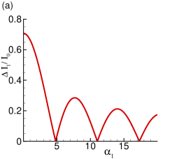
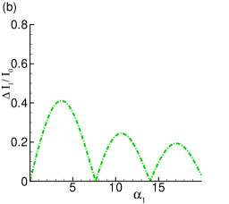
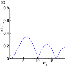
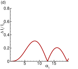
Figure 13: The dependence of the Shapiro step width for $p$-wave JJs at $\alpha={\bf B}=h=0$ on the amplitude of the $ac$-voltage $\alpha_{1}=2eV_{1}/(\hbar\omega)$ at (a) $n_{0}=0$, (b) $n_{0}=1$, (c) $n_{0}=2$, and (d) $n_{0}=3$. $D$ is chosen to be $D=0.5$.

where we have used the fact that the maximum width of the step occurs at $\varphi_{0}=\varphi_{0}^{m}=\pi$. The dependence of the step width on $\alpha_{1}$ for different values of $n_{0}=0,1,2,3$ is presented in Fig. 13.

Next, we apply this procedure for the case where $B=h=0$ but $\alpha\neq 0$. The Andreev bound state energy is given by Eq. (45) and consists of four branches, i.e. each electron and hole branch is split into two states. One of these split states, corresponding to the $+$ sign (Eq. 45) are independent of $\alpha$. For these two states, the AC Josephson current can be easily shown to be given by Eq. (LABEL:ac1); the corresponding Shapiro step width is given by Eq. (65). In contrast, the energy dispersion of the other two branches with designated by $-$ sign (Eq. 45) depend on the ratio $\alpha/v_{F}$ and can be rewritten as

$$E_{-}^{s} = \frac{s\Delta_{0}\beta\sqrt{D}\cos(\phi/2)}{\sqrt{1-D(1-\beta^{2})\cos^{2}(\phi/2)}}$$ (66)

where $\beta=(1-\alpha/v_{F})/(1+\alpha/v_{F})$. We note that these branches do not contribute to the Josephson current if $\alpha=v_{F}$. For $\alpha<v_{F}$ the contribution from the $s=-$ branch to the current is given by,

$$I_{J2}^{\rm AC} = \frac{I_{0}\beta\sqrt{D}}{2}\frac{\sum_{n}J_{n}(\alpha_{1}/2)\sin[(\varphi_{0}+(\omega_{J}-2n\omega)t)/2]}{\left\{1-D_{0}-D_{0}\sum_{n}J_{n}(\alpha_{1})\cos[\varphi_{0}+(\omega_{J}-n\omega)t]\right\}^{3/2}}$$ (67)

where $D_{0}=D(1-\beta^{2})/2$. The Shapiro step width corresponding to $n=n_{0}$ is given by

$$\Delta I_{2} = I_{0}\sqrt{D}\beta\left|\frac{J_{n_{0}}[\alpha_{1}/2]\sin(\phi_{0}^{m}/2)}{\left\{1-D_{0}-D_{0}J_{n_{0}}(\alpha_{1})\cos(\phi_{0}^{m})\right\}^{3/2}}\right|$$

In order to determine $\phi_{0}^{m}$, we need to find the value of $\varphi_{0}$ which maximizes the Shapiro step width. This can be computed easily from Eq. (67) by maximizing the current after setting $\omega_{J}=2n_{0}\omega$. This procedure yields

$$\phi_{0}^{m} = 2\arcsin\left[\sqrt{(1-2D_{0})/(4D_{0})}\right]\quad{\rm if}\,\,D_{0}>1/6$$ (69)

$$= \pi\quad{\rm otherwise}$$

The dependence of the Shapiro step width on $\alpha_{1}$ (Eq. (LABEL:shap2)) is plotted, using Eq. (69) in Fig. (14) for $D_{0}<1/6$ (Fig. 14(a)) and $D_{0}>1/6$ (Fig. 14(b)). We note that Eqs. (LABEL:shap2) and (69) allow one to obtain the strength of the spin-orbit coupling in these JJs from the Shapiro step width.

Next we consider the case where $\alpha=B=0$ and $h\neq 0$. Here the energy dispersion corresponds to four branches as can be seen from Eq. (46). We first consider the branches corresponding to $E_{\uparrow\downarrow}^{-}$. Here we note that when $E_{\uparrow\downarrow}^{-}(s=\pm)<0$, the Josephson currents from these two branches cancel each other. Similarly, if $E_{\uparrow\downarrow}^{-}(s=\pm)>0$, none of the branches contribute at $T=0$. Thus these branches contribute to the Josephson current for $\sqrt{D}\sqrt{\Delta^{2}-4h^{2}}|\cos(\varphi/2)|>h$; the presence/absence of Josephson currents from these branches can therefore be used to estimate $D$ in these junctions, provided $\Delta$ and $h$ are known. The Josephson current from these branches and the corresponding Shapiro step widths (when the above-mentioned condition is satisfied) are given by Eq. (LABEL:ac1) and (65) respectively. In contrast, the contribution from the branches corresponding to $E_{\uparrow\downarrow}^{+}(s)$ are given by

$$I_{J3}^{\rm AC}/I_{0} = -\frac{2e}{\hbar}\left[Dh\sin\phi(t)+\sum_{s=\pm}\frac{s\sqrt{D}(\Delta^{2}-4h^{2}+4Dh(1+\cos\phi(t)))\sin[\phi(t)/2]}{\left[\Delta^{2}-4h^{2}+2hD(1+\cos(\phi(t)/2))\right]^{1/2}}\theta(-E_{\uparrow\downarrow}^{-}(s))\right]$$ (70)

We note that when both $E^{-}_{\uparrow\downarrow}(s=\pm)<0$, the Josephson current is purely $2\pi$ periodic and is given by

$$I_{J4}^{\rm AC} = -\frac{I_{0}Dh}{\Delta}\sum_{n}J_{n}(\alpha_{1})\sin[\varphi_{0}+(\omega_{J}-n\omega)t]$$ (71)

In this case one has both odd and even Shapiro steps with the step width $\Delta I_{4}[n_{0}]=|I_{0}DhJ_{n_{0}}(\alpha_{1})/\Delta|$. However, for $E_{\uparrow\downarrow}^{-}(s=+)>0$ and $E_{\uparrow\downarrow}^{-}(s=-)<0$, one has

$$I_{J5}^{\rm AC} = I_{J4}^{\rm AC}+\frac{\sqrt{D}[\Delta^{2}-4h^{2}+4Dh+4Dh\sum_{n}J_{n}(\alpha_{1})\cos(\phi_{0}+(\omega_{J}-n\omega)t)]\sum_{n}J_{n}(\alpha_{1}/2)\sin[(\phi_{0}+(\omega_{J}-2n\omega)t)/2]}{\left[\Delta^{2}-4h^{2}+2hD+2hD\sum_{n}J_{n}(\alpha_{1})\cos(\phi_{0}+(\omega_{J}-n\omega)t)\right]^{1/2}}$$

We note that in this case the JJ will have both $2\pi$ periodic and $4\pi$ periodic components. The corresponding Shapiro step width is given for $n=n_{0}$

$$\Delta I_{5} = \Delta I_{4}[n_{0}]\quad n_{0}=2m_{0}+1$$

$$= \Delta I_{4}[n_{0}]\left|\sin[\varphi_{0}^{m}]\right|+\left|\frac{\sqrt{D}[\Delta^{2}-4h^{2}+4Dh+4DhJ_{n_{0}}(\alpha_{1})\cos\phi_{0}]J_{n_{0}}(\alpha_{1}/2)\sin\phi_{0}/2}{\left[\Delta^{2}-4h^{2}+2hD+2hDJ_{n_{0}}(\alpha_{1})\cos\phi_{0}\right]^{1/2}}\right|\quad n_{0}=2m_{0}$$

where $m_{0}$ is an integer and $\varphi_{0}^{m}$ denotes the value of $\varphi_{0}$ for which the stepwidth is maximum. This value needs to be numerically determined for the present case by minimizing Eq. (LABEL:ac5) at $\omega_{J}=2n_{0}\omega$ with respect to $\varphi_{0}$.

Finally, we treat the case $B,h\neq 0$ and $\alpha=0$. Here the Andreev bound states are given by Eq. (47) and (48). For $E\equiv E_{\uparrow\downarrow}^{\pm}(s)$ (Eq. (47)), there are four branches. For $E=E^{+}_{\uparrow\downarrow}$ both the branches are above the Fermi energy if $\sqrt{B^{2}+h^{2}}\geq\Delta\sqrt{D}$. In this case, there is no Josephson current contribution from these branches. Similarly, for $E=E^{-}_{\uparrow\downarrow}$, the same condition results in both the branches being below the Fermi level. In this case, their contribution to the Josephson currents cancel each other. Thus the contribution to the Josephson current from $E_{\uparrow\downarrow}$ occurs only when $\sqrt{B^{2}+h^{2}}<\Delta\sqrt{D}$. However, even in this case, the contribution to the Josephson currents from the positive ($E^{+}$) and negative ($E^{-}$) branches cancel each other and the net Josephson current vanishes. A similar results can be easily deduced for $E=E_{\uparrow\uparrow}^{\pm}$ (Eq. (48)) and $E_{\downarrow\uparrow}$ (Eq. (49)) branches.

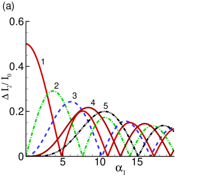
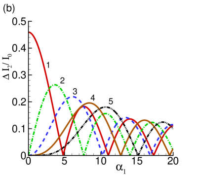
Figure 14: The dependence of the Shapiro step width for $p$-wave JJs at ${\bf B}=h=0$ and $\alpha\neq 0$ on the amplitude of the $ac$-voltage $\alpha_{1}=2eV_{1}/(\hbar\omega)$ according to Eq.(67) for two different values of the parameter $D_{0}$, (a) $D_{0}=1/8<1/6$ at $D=0.5$ and $\beta=\sqrt{0.5}$, corresponding to $\phi_{0}^{m}=\pi$ and (b) $D_{0}=7/40>1/6$ at $D=0.5$ and $\beta=\sqrt{0.3}$. The curves in each figure are drawn by (1) solid red curve at $n_{0}=0$, (2) green dot-dashed curve at $n_{0}=1$, (3) blue dashed curve at $n_{0}=2$, (4) brown dotted curve at $n_{0}=3$, and (5) black double dot-dashed curve at $n_{0}=4$.

VI Conclusion

In this paper we study the Josephson current between 1D nanowires of $p$-wave superconductors separated by an insulating barrier in the presence of Rashba SOI and the magnetic fields ${\bf B}$ and $h$. The presence of the SOI and Zeeman magnetic fields enlarges the standard two-component $BdG$ system equations to four-component system equations (13)- (16) for new BdG wave vector $\eta_{a}(x)=\left(\eta_{a,\uparrow,+}^{{\dagger}}(x),\eta_{a,\downarrow,+}^{{\dagger}}(x),\eta_{a,\downarrow,-}(x),\eta_{a,\uparrow,-}(x)\right)$. The BdG equations (13)-(16) coincide with the standard BdG equations in the absence of the in-plane magnetic field ${\bf B}$, which provide only one relation $\eta^{\ast}_{a,\sigma,b}/\eta_{a,{\bar{\sigma}},{\bar{b}}}$ between quasi-particle and quasi-hole states, where $\sigma=\uparrow,\downarrow$ and ${\bar{\sigma}}=\downarrow,\uparrow$. Instead, the BdG equations (13)-(16) in the presence of ${\it in-plane}$ magnetic field ${\bf B}$ and Rashba SOI provide three relations $\eta^{\ast}_{a,\sigma,b}/\eta_{a,{\bar{\sigma}},{\bar{b}}}$, $\eta^{\ast}_{a,\sigma,b}/\eta_{a,\sigma,{\bar{b}}}$, and $\eta_{a,\sigma,b}/\eta_{a,{\bar{\sigma}},b}$ between the quasi-particle and quasi-hole states, corresponding to new Andreev scattering channels. We studied in this paper all these scattering channels in detail by generalizing the method of Ref. ksy04, for study of Josephson junction with $\delta$-function insulator between two $p$-wave superconductors to systems with SOI and Zeeman fields. We have shown in this paper that $\pi$-state is realized in Josephson junction with $p$-wave superconductors. Moreover, we have demonstrated the existence of magneto-Josephson effect in these systems. We note that although the existence of the magneto-Josephson effect in a topological superconductor has been predicted recently jpar13 ; kss12 ; pjpa13 , the question of whether this effect is observable in superconducting junctions with $p$-wave superconductors and the presence of SOI was not addressed before. We have predicted in the paper new Andreev-type tunneling channels for quasi-particles and quasi-holes which are responsible to the magneto-Josephson effect.

In conclusion, we have studied Josephson effect in a junction between two $p$-wave 1D nanowires in the presence of SOI and Zeeman fields. We have analyzed the Josephson current in these junctions and provided analytical expressions of the Andreev bound states in several limiting cases. We have also demonstrated the presence of magneto-Josephson effect in these junctions. Our heoretical predictions are shown to be verifiable by straightforward experiments on these systems.

Appendix A Andreev bound state energies at ${\bf B}\neq 0$

Andreev bound state energies are obtained from the conditions $F_{\uparrow\downarrow}^{\ast}(E_{\uparrow\downarrow})=0$, $F_{\uparrow\uparrow}^{\ast}(E_{\uparrow\uparrow})=0$, $F_{\uparrow\downarrow}({\tilde{E}}_{\uparrow\downarrow})=0$ corresponding to three channels, and also from the conditions, obtained by interchanging the spin orientations as $F_{\downarrow\uparrow}^{\ast}(E_{\downarrow\uparrow})=0$, $F_{\downarrow\downarrow}^{\ast}(E_{\downarrow\downarrow})=0$, $F_{\downarrow\uparrow}({\tilde{E}}_{\downarrow\uparrow})=0$.

Andreev bound state energy $E_{\uparrow\downarrow}$ is obtained from the condition $F_{\uparrow\downarrow}^{\ast}(E_{\uparrow\downarrow})=0$ with the expression (36) yielding

$$\left\{(E_{\uparrow\downarrow}+h)\left[(E_{\uparrow\downarrow}-h)^{2}+k^{2}(v_{F}+\alpha)^{2}+B^{2}-\Delta^{2}\right]^{2}-2B^{2}E_{\uparrow\downarrow}\right\}^{2}\left(1-D\cos^{2}\frac{\varphi}{2}\right)-$$

$$\left\{k(v_{f}-\alpha)\left[(E_{\uparrow\downarrow}-h)^{2}+k^{2}(v_{F}+\alpha)^{2}+B^{2}-\Delta^{2}\right]+2kB^{2}\alpha\right\}^{2}D\cos^{2}\frac{\varphi}{2}=0.$$ (74)

This expressin depends apart from the parameters $\alpha$, ${\bf B}$, and $h$ also on the momentum $k^{2}$. Expression for $k^{2}_{\pm}$, obtained from the energy spectrum (10), reads

$$k^{2}_{\pm}(v_{F}^{2}-\alpha^{2})^{2}=(E^{2}-h^{2}-B^{2}-\Delta^{2})(v_{F}^{2}-\alpha^{2})-2(Ev_{F}+\alpha h)^{2}+2\Delta^{2}v_{F}^{2}\pm\Big{\{}\big{[}(E^{2}-h^{2}-B^{2}-\Delta^{2})(v_{F}^{2}-\alpha^{2})-$$

$$2(Ev_{F}+\alpha h)^{2}+2\Delta^{2}v_{F}^{2}\big{]}^{2}-\left[(E^{2}-h^{2}-B^{2}-\Delta^{2})^{2}-4\Delta^{2}(h^{2}+B^{2})\right](v_{F}^{2}-\alpha^{2})^{2}\Big{\}}^{1/2}.$$ (75)

Elimination of $k^{2}$, by substituting it from (75) into Eq. (74), yields a general expression to find $E_{\uparrow\downarrow}$, which is not easy to solve exactly.

The condition $F_{\uparrow\uparrow}^{\ast}(E_{\uparrow\uparrow})=0$ with the expression (39) yields

$$k^{2}(Ev_{F}+\alpha h)^{2}-\Delta^{2}(E^{2}_{\uparrow\uparrow}+\alpha^{2}k^{2})+\Delta^{2}D(E^{2}_{\uparrow\uparrow}+\alpha^{2}k^{2})\cos^{2}\frac{\varphi-\theta}{2}=0.$$ (76)

Routine calculations, after substitution of $k^{2}$ from Eq. (75) to this equation, result in

$$\left\{(v_{F}^{2}-\alpha^{2})E^{2}_{\uparrow\uparrow}\Delta^{2}\left(1-D\cos^{2}\frac{\varphi-\theta}{2}\right)-(E^{2}_{\uparrow\uparrow}+\Delta^{2}-B^{2}-h^{2})\left[(E_{\uparrow\uparrow}v_{F}+\alpha h)^{2}-\alpha^{2}\Delta^{2}\left(1-D\cos^{2}\frac{\varphi-\theta}{2}\right)\right]\right\}^{2}-$$

$$4E^{2}_{\uparrow\uparrow}\Delta^{2}D\cos^{2}\frac{\varphi-\theta}{2}(E_{\uparrow\uparrow}v_{F}+\alpha h)^{2}\left[(E_{\uparrow\uparrow}v_{F}+\alpha h)^{2}-\alpha^{2}\Delta^{2}\left(1-D\cos^{2}\frac{\varphi-\theta}{2}\right)\right]=0$$ (77)

This equation can be solved numerically for a general case when $\alpha,~{}{\bf B},~{}h\neq 0$. The expression for $F_{\downarrow\downarrow}^{\ast}(E_{\downarrow\downarrow})=0$ is obtained from Eq. (77) by interchanging $\alpha\to-\alpha$, $h\to-h$, and $\theta\to-\theta$.

The bound state energy in the particle-particle channel with opposite spin orientations is determined from the condition $F_{\uparrow\downarrow}(E^{\prime}_{\uparrow\downarrow})=0$, which can be written by using the expression (42) for $F_{\downarrow\uparrow}$ as,

$$\alpha^{2}k^{2}-\left(E^{{}^{\prime}2}_{\uparrow\downarrow}+\alpha^{2}k^{2}\right)D\sin^{2}\frac{\theta}{2}=0.$$ (78)

Substituting $k^{2}$ from Eq. (75) to this equation yields the equation to determine $E^{\prime}_{\uparrow\downarrow}$,

$$\alpha^{4}\left[(E_{\uparrow\downarrow}^{{}^{\prime}2}+\Delta^{2}-B^{2}-h^{2})^{2}-4\Delta^{2}E^{{}^{\prime}2}_{\uparrow\downarrow}\right]+2\alpha^{2}D\sin^{2}\frac{\theta}{2}\Big{\{}v_{F}^{2}E^{{}^{\prime}4}_{\uparrow\downarrow}+(v_{F}^{2}-\alpha^{2})\Delta^{2}E^{{}^{\prime}2}_{\uparrow\downarrow}+(v_{F}^{2}+\alpha^{2})B^{2}E^{{}^{\prime}2}_{\uparrow\downarrow}+$$

$$(v_{F}^{2}+3\alpha^{2})h^{2}E^{{}^{\prime}2}_{\uparrow\downarrow}-4v_{F}\alpha hE^{{}^{\prime}3}+\alpha^{2}(\Delta^{2}-B^{2}-h^{2})^{2}\Big{\}}+D^{2}\sin^{4}\frac{\theta}{2}\Big{\{}v_{F}^{2}(v_{F}^{2}-4\alpha^{2})E^{{}^{\prime}4}_{\uparrow\downarrow}+$$

$$2\alpha^{2}E^{{}^{\prime}2}_{\uparrow\downarrow}\left[v_{F}^{2}\Delta^{2}-v_{F}^{2}B^{2}-(v_{F}^{2}+2\alpha^{2})h^{2}\right]-8\alpha^{3}v_{F}hE^{{}^{\prime}3}_{\uparrow\downarrow}+\alpha^{4}(\Delta^{2}-B^{2}-h^{2})^{2}\Big{\}}=0.$$ (79)

Note that the condition $F_{\downarrow\uparrow}(E^{\prime}_{\downarrow\uparrow})=0$ provides for $E^{\prime}_{\downarrow\uparrow}$ exactly the same expression as (79), i. e. $E^{\prime}_{\downarrow\uparrow}=E^{\prime}_{\uparrow\downarrow}$. Indeed, a reality of this fact can be tested according to the rule that interchanging the spin directions is equivalent to the replacements of $\alpha\to-\alpha$, $h\to-h$, and $\theta\to-\theta$.

References

- (1) A.Yu. Kitaev, Phys. Usp. 44, 131 (2001).
- (2) A. Yu. Kitaev, Annals Phys. 303, 2 (2003).
- (3) R. M. Lutchyn, J. D. Sau, and S. Das Sarma, Phys. Rev. Lett. 105, 077001 (2010).
- (4) Y. Oreg, G. Refael, and F. von Oppen, Phys. Rev. Lett. 105, 177002 (2010).
- (5) N. Read and D. Green, Phys. Rev. B 61, 10267 (2000).
- (6) D. A. Ivanov, Phys. Rev. Lett. 86, 268 (2001).
- (7) J. Alicea, Y. Oreg, G. Refael, F. von Oppen, and M. P. A. Fisher, Nat. Phys. 7, 412 (2011).
- (8) L. P. Gor’kov and E. I. Rashba, Phys. Rev. Lett. 87, 037004 (2001).
- (9) X. Liu, J. K. Jain, and C. X. Liu, Phys. Rev. Lett. 113, 227002 (2014).
- (10) C. R. Reeg and D. L. Maslov, Phys. Rev. B 92, 134512 (2015).
- (11) T. Yu and M. W. Wu, Phys. Rev.B 93, 195308 (2016).
- (12) V. M. Edelstein, Zh. Eksp. Teor. Fiz. 95, 2151 (1989) [Sov. Phys. JETP 68, 1244 (1989)].
- (13) P. A. Frigeri, D. F. Agterberg, A. Koga, and M. Sigrist, Phys. Rev. Lett. 92, 097001 (2004).
- (14) H. -J. Kwon, K. Sengupta, and V. M. Yakovenko, Eur. Phys. J. B 37, 349 (2004).
- (15) L. Fu and C. L. Kane, Phys. Rev. B 79, 161408 (2009).
- (16) L. Jiang, D. Pekker, J. Alicea, G. Refael, Y. Oreg, and F. von Oppen, Phys. Rev. Lett. 107, 236401 (2011).
- (17) L. Jiang, D. Pekker, J. Alicea, G. Refael, Y. Oreg, A. Brataas, and F. von Oppen, Phys. Rev. B 87, 075438 (2013); S. Jacobsen, I. Kulagina, and J. Linder, Sci. Rep. 6, 23926 (2016).
- (18) E. Nakhmedov, O. Alekperov, F. Tatardar, Yu. M. Shukrinov, I. Rahmonov, and K. Sengupta, Phys. Rev. B 96, 014519 (2017).
- (19) F. S. Nogueira and K. H. Bennemann, Europhys. Lett. 67, 620 (2004).
- (20) Y. Asano, Phys. Rev. B 74, 220501 (2006).
- (21) P. M. R. Brydon, Phys. Rev. B 80, 224520 (2009).
- (22) P. M. R. Brydon, Y. Asano, and C. Timm, Phys. Rev. B 83, 180504 (2011).
- (23) H. Zhang, K. S. Chan, Z. Lin, and J. Wang, Phys. Rev. B 85 024501 (2012).
- (24) L. Klam, A. Epp, W. Chen, M. Sigrist, and D. Manske, Phys. Rev. B 89, 174505 (2014).
- (25) L. Elster, M. Houzet, and J. S. Meyer, Phys. Rev. B 93, 104519 (2016)
- (26) A. G. Bauer and B. Sothmann, Phys. Rev. B 99, 214508 (2019).
- (27) M. T. Mercaldo, P. Kotetes, and M. Cuoco, Phys. Rev. B 100, 104519 (2019).
- (28) A. J. Leggett, Rev. Mod. Phys. 47, 331 (1975).
- (29) V. P. Mineev and K. V. Samochin, Introduction to the theory of unconventioal superconductivity, Moscow Engeneering-Technical Institute Press, Moscow 1998, p. 144, ISBN 5-89155-024-5.
- (30) J. Nilsson, A. R. Akhmerov, and C. W. J. Beenakker, Phys. Rev. Lett. 101, 120403 (2008).
- (31) T. Birol and P. W. Brouwer, Phys. Rev. B 80, 014434 (2009).
- (32) P. Kotetes, G. Schön, and A. Shnirman, J. Korean Phys. Soc. 62, 1558 (2013).
- (33) F. Pientika, L. Jiang, D. Pekker, J. Alicea, G. Refael, Y. Oreg, and F. von Oppen, New J. Physics 15, 115001 (2013).