Scalable methods for computing state similarity in
deterministic Markov Decision Processes

Pablo Samuel Castro
Google Brain
psc@google.com
Abstract

We present new algorithms for computing and approximating bisimulation metrics in Markov Decision Processes (MDPs). Bisimulation metrics are an elegant formalism that capture behavioral equivalence between states and provide strong theoretical guarantees on differences in optimal behaviour. Unfortunately, their computation is expensive and requires a tabular representation of the states, which has thus far rendered them impractical for large problems. In this paper we present a new version of the metric that is tied to a behavior policy in an MDP, along with an analysis of its theoretical properties. We then present two new algorithms for approximating bisimulation metrics in large, deterministic MDPs. The first does so via sampling and is guaranteed to converge to the true metric. The second is a differentiable loss which allows us to learn an approximation even for continuous state MDPs, which prior to this work had not been possible.

Introduction

A finite Markov Decision Process (MDP) is defined as a 5-tuple $\mathcal{M}=\langle\mathcal{S},\mathcal{A},\mathcal{P},\mathcal{R},\gamma\rangle$, where $\mathcal{S}$ is a finite set of states, $\mathcal{A}$ is a finite set of actions, $\mathcal{P}:\mathcal{S}\times\mathcal{A}\rightarrow\Delta(\mathcal{S})$ is the next state transition function (where $\Delta(X)$ is the probability simplex over the set $X$), $\mathcal{R}:\mathcal{S}\times\mathcal{A}\rightarrow\mathbb{R}$ is the reward function (assumed to be bounded by $R_{max}$), and $\gamma\in[0,1)$ is a discount factor. An MDP is the standard formalism for expressing sequential decision problems, typically in the context of planning or reinforcement learning (RL). The set of states $\mathcal{S}$ is one of the central components of this formalism, where each state sโˆˆ๐’ฎ๐‘ ๐’ฎs\in\mathcal{S} is meant to encode sufficient information about the environment such that an agent can learn how to behave in a consistent manner. Figureย 1 illustrates a simple MDP where each cell represents a state.

Refer to caption
Figure 1: A grid MDP (bottom) with a copy of itself (top). The goal of an agent is to find the shortest path to the green cells. At each iteration, the agent has a 50% chance of jumping to the other level.

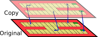
There is no canonical way of defining the set of states for a problem. Indeed, improperly designed state spaces can have drastic effects on the algorithm used. Consider the grid MDP in the bottom of Figureย 1, where an agent must learn how to navigate to the green cells, and imagine we create an exact replica of the MDP such that the agent randomly transitions between the two layers for each move. By doing so we have doubled the number of states and the complexity of the problem. However, from a planning perspective the two copies of each state should be indistinguishable. A stronger notion of state identity is needed that goes beyond the labeling of states and which is able to capture behavioral indistinguishability.

In this paper we explore notions of behavioral similarity via state pseudometrics111A pseudometric is a metric $d$ where $\forall s,t\in\mathcal{S}.\quad s=t\implies d(s,t)=0$, but not the converse. $d:\mathcal{S}\times\mathcal{S}\rightarrow\mathbb{R}$, and in particular those which assign a distance of 00 to states that are behaviorally indistinguishable. Pseudometrics further allow us to reason about states based on what we may know about other similar states. This is a common use-case in fields such as formal verification, concurrency theory, and in safe RL, where one may want to provide (non-)reachability guarantees. In the context of planning and reinforcement learning, these can be useful for state aggregation and abstraction.

Our work builds on bisimulation metrics (?) which provide us with theoretical guarantees such as states that are close to each other (with respect to the metric) will have similar optimal value functions. These theoretical properties render them appealing for planning and learning, and they have previously been used for state aggregation (?;ย ?), policy transfer (?), representation discovery (?), and exploration (?).

Unfortunately, these metrics are expensive to compute (?) and require fully enumerating the states, even when using sampling-based approximants (?), on-the-fly approximants (?;ย ?), or approximants which exploit structure in the state space (?). The full-state enumeration requirement has thus far rendered bisimulation metrics impractical in problems with large state spaces, and completely incompatible with continuous state spaces. Additionally, bisimulation metrics can be overly pessimistic in the sense that they consider worst-case differences between states. Although desirable for certain applications, such as in guaranteeing safe behaviors, it can prove overly restrictive for many practical problems of interest.

In this paper we address these impracticalities with the following key contributions:

  1. 1.

    An on-policy variant of bisimulation which focuses only on the behavior of interest, rather than worst-case scenarios, along with an analysis of its theoretical properties.

  2. 2.

    A new sampling-based online algorithm for exact computation of the original and on-policy bisimulation metrics with guaranteed convergence.

  3. 3.

    A differentiable loss function for learning an approximation of the two bisimulation metrics using neural networks. We provide empirical evidence of this learning algorithm on MDPs with large and continuous state spaces. To the best of the authorโ€™s knowledge, this is the first work proposing a mechanism for approximating bisimulation metrics with neural networks.

Background

Given an MDP $\mathcal{M}$, a policy $\pi:\mathcal{S}\rightarrow\Delta(\mathcal{A})$ induces a corresponding state-value function $V^{\pi}:\mathcal{S}\rightarrow\mathbb{R}$ (?): Vฯ€โ€‹(s)=๐”ผaโˆผฯ€โ€‹(s)โ€‹[โ„›โ€‹(s,a)+ฮณโ€‹๐”ผsโ€ฒโˆผ๐’ซโ€‹(s,a)โ€‹Vฯ€โ€‹(sโ€ฒ)]superscript๐‘‰๐œ‹๐‘ subscript๐”ผsimilar-to๐‘Ž๐œ‹๐‘ delimited-[]โ„›๐‘ ๐‘Ž๐›พsubscript๐”ผsimilar-tosuperscript๐‘ โ€ฒ๐’ซ๐‘ ๐‘Žsuperscript๐‘‰๐œ‹superscript๐‘ โ€ฒV^{\pi}(s)=\mathbb{E}_{a\sim\pi(s)}\left[\mathcal{R}(s,a)+\gamma\mathbb{E}_{s^{\prime}\sim\mathcal{P}(s,a)}V^{\pi}(s^{\prime})\right]. In the control setting, we are typically in search of the optimal value functionย (?):
Vโˆ—โ€‹(s)=maxaโˆˆ๐’œโก[โ„›โ€‹(s,a)+ฮณโ€‹๐”ผsโ€ฒโˆผ๐’ซโ€‹(s,a)โ€‹Vโˆ—โ€‹(sโ€ฒ)]superscript๐‘‰๐‘ subscript๐‘Ž๐’œโ„›๐‘ ๐‘Ž๐›พsubscript๐”ผsimilar-tosuperscript๐‘ โ€ฒ๐’ซ๐‘ ๐‘Žsuperscript๐‘‰superscript๐‘ โ€ฒV^{*}(s)=\max_{a\in\mathcal{A}}\left[\mathcal{R}(s,a)+\gamma\mathbb{E}_{s^{\prime}\sim\mathcal{P}(s,a)}V^{*}(s^{\prime})\right].

Bisimulation relations, originally introduced in the field of concurrency theory, were adapted for MDPs by ? (?), capture a strong form of behavioral equivalence: if s,tโˆˆ๐’ฎ๐‘ ๐‘ก๐’ฎs,t\in\mathcal{S} are bisimilar, then Vโˆ—โ€‹(s)=Vโˆ—โ€‹(t)superscript๐‘‰๐‘ superscript๐‘‰๐‘กV^{*}(s)=V^{*}(t).

Definition 1.

Given an MDP $\mathcal{M}$, an equivalence relation $E\subseteq\mathcal{S}\times\mathcal{S}$ is a bisimulation relation if whenever (s,t)โˆˆE๐‘ ๐‘ก๐ธ(s,t)\in E the following properties hold, where $\mathcal{S}_{E}$ is the state space $\mathcal{S}$ partitioned into equivalence classes defined by $E$:

  1. 1.

    โˆ€aโˆˆ๐’œ,โ„›โ€‹(s,a)=โ„›โ€‹(t,a)formulae-sequencefor-all๐‘Ž๐’œโ„›๐‘ ๐‘Žโ„›๐‘ก๐‘Ž\forall a\in\mathcal{A},\mathcal{R}(s,a)=\mathcal{R}(t,a)

  2. 2.

    โˆ€aโˆˆ๐’œ,โˆ€cโˆˆ๐’ฎE,๐’ซโ€‹(s,a)โ€‹(c)=๐’ซโ€‹(t,a)โ€‹(c)formulae-sequencefor-all๐‘Ž๐’œformulae-sequencefor-all๐‘subscript๐’ฎ๐ธ๐’ซ๐‘ ๐‘Ž๐‘๐’ซ๐‘ก๐‘Ž๐‘\forall a\in\mathcal{A},\forall c\in\mathcal{S}_{E},\mathcal{P}(s,a)(c)=\mathcal{P}(t,a)(c), where ๐’ซโ€‹(s,a)โ€‹(c)=โˆ‘sโ€ฒโˆˆc๐’ซโ€‹(s,a)โ€‹(sโ€ฒ)๐’ซ๐‘ ๐‘Ž๐‘subscriptsuperscript๐‘ โ€ฒ๐‘๐’ซ๐‘ ๐‘Žsuperscript๐‘ โ€ฒ\mathcal{P}(s,a)(c)=\sum_{s^{\prime}\in c}\mathcal{P}(s,a)(s^{\prime}),

Two states s,tโˆˆ๐’ฎ๐‘ ๐‘ก๐’ฎs,t\in\mathcal{S} are bisimilar if there exists a bisimulation relation $E$ such that (s,t)โˆˆE๐‘ ๐‘ก๐ธ(s,t)\in E. We denote the largest222Note that there can be a number of equivalence relations satisfying these properties. The smallest is the identity relation, which is vacuously a bisimulation relation. bisimulation relation as $\sim$.

Equivalence relations can be brittle: they require exact equivalence under probabilistic transitions. This can be especially problematic if we are estimating transition probabilities from data, as it is highly unlikely they will match exactly.

Extending the work of ? (?) for labeled Markov processes, ? (?) generalized the notion of MDP bisimulation relations to metrics, yielding a smoother notion of similarity than equivalence relations. Let $\mathbb{M}$ be the set of all pseudometrics on $\mathcal{S}$. A pseudometric $d\in\mathbb{M}$ induces an equivalence relation Ed:={(s,t)|dโ€‹(s,t)=0}assignsubscript๐ธ๐‘‘conditional-set๐‘ ๐‘ก๐‘‘๐‘ ๐‘ก0E_{d}:=\{(s,t)|d(s,t)=0\}. That is, any two states with distance 00 will be collapsed onto the same equivalence class.

Definition 2.

(?) A pseudometric $d\in\mathbb{M}$ is a bisimulation metric if $E_{d}$ is $\sim$.

Bisimulation metrics use the 1-Wasserstein metric $\mathcal{W}_{1}:\mathbb{M}\rightarrow\mathbb{P}$, where $\mathbb{P}$ is the set of all metrics between probability distributions over $\mathcal{S}$. Given two state distributions $X,Y\in\Delta(\mathcal{S})$ and a pseudometric $d\in\mathbb{M}$, the Wasserstein $\mathcal{W}_{1}(d)(X,Y)$ can be expressed by the following (primal) linear program (LP), which โ€œliftsโ€ a pseudometric $d\in\mathbb{M}$ onto one in $\mathbb{P}$ (?):

maxuโˆˆโ„|๐’ฎ|โ€‹โˆ‘sโˆˆ๐’ฎ(Xโ€‹(s)โˆ’Yโ€‹(s))โ€‹ussubscriptusuperscriptโ„๐’ฎsubscript๐‘ ๐’ฎ๐‘‹๐‘ ๐‘Œ๐‘ subscript๐‘ข๐‘ \displaystyle\max_{\textbf{u}}\in\mathbb{R}^{|\mathcal{S}|}\sum_{s\in\mathcal{S}}\left(X(s)-Y(s)\right)u_{s} (1)
โˆ€s,sโ€ฒโˆˆ๐’ฎ,ย โ€‹usโˆ’usโ€ฒโ‰คdโ€‹(s,sโ€ฒ)formulae-sequencefor-all๐‘ superscript๐‘ โ€ฒ๐’ฎย subscript๐‘ข๐‘ subscript๐‘ขsuperscript๐‘ โ€ฒ๐‘‘๐‘ superscript๐‘ โ€ฒ\displaystyle\forall s,s^{\prime}\in\mathcal{S},\textrm{ }u_{s}-u_{s^{\prime}}\leq d(s,s^{\prime})
$\displaystyle 0\leq\textbf{u}\leq 1$
Theorem 1.

(?): Define $\mathcal{F}:\mathbb{M}\rightarrow\mathbb{M}$ by

$\displaystyle\mathcal{F}$ (d)โ€‹(s,t)=๐‘‘๐‘ ๐‘กabsent\displaystyle(d)(s,t)= (2)
maxaโˆˆ๐’œโก(|โ„›โ€‹(s,a)โˆ’โ„›โ€‹(t,a)|+ฮณโ€‹๐’ฒ1โ€‹(d)โ€‹(๐’ซโ€‹(s,a),๐’ซโ€‹(t,a)))subscript๐‘Ž๐’œโ„›๐‘ ๐‘Žโ„›๐‘ก๐‘Ž๐›พsubscript๐’ฒ1๐‘‘๐’ซ๐‘ ๐‘Ž๐’ซ๐‘ก๐‘Ž\displaystyle\max_{a\in\mathcal{A}}\left(\left|\mathcal{R}(s,a)-\mathcal{R}(t,a)\right|+\gamma\mathcal{W}_{1}(d)(\mathcal{P}(s,a),\mathcal{P}(t,a))\right)

then $\mathcal{F}$ has a unique fixed point, $d_{\sim}$, and $d_{\sim}$ is a bisimulation metric.

The operator $\mathcal{F}$ can be used to iteratively compute a bisimulation metric as follows. Starting from an initial estimate $d_{0}$, we can compute $d_{n+1}=\mathcal{F}(d_{n})=\mathcal{F}^{n+1}(d_{0})$. By iteratively applying $\mathcal{F}$ $\lceil\frac{\ln\delta}{\ln\gamma}\rceil$ times, one can compute $d_{\sim}$ up to an accuracy $\delta$, with an overall complexity of $O\left(|\mathcal{A}||\mathcal{S}|^{4}\log|\mathcal{S}|\frac{\ln\delta}{\ln\gamma}\right)$.

On-policy bisimulation

The strong theoretical guarantees of bisimulation relations and metrics are largely due to their inherent โ€œpessimismโ€: they consider equivalence under all actions, even pathologically bad ones (i.e. actions that never lead to positive outcomes for the agent). Indeed, there exist systems where Vโˆ—โ€‹(s)=Vโˆ—โ€‹(t)superscript๐‘‰๐‘ superscript๐‘‰๐‘กV^{*}(s)=V^{*}(t), but dโˆผโ€‹(s,t)subscript๐‘‘similar-to๐‘ ๐‘กd_{\sim}(s,t) can be arbitrarily large, providing no useful bounds on the optimal behaviour from s๐‘ s and $t$ (see Figureย 2). ? (?) also demonstrated that this pessimism yields poor results when using bisimulation metrics for policy transfer.

s๐‘ s$t$ $u$a, [K]bb, [K]a
Figure 2: Edge labels indicate action ($\{a,b\}$) and non-zero rewards ($[K]$). When $\gamma=0.9$, Vโˆ—โ€‹(s)=Vโˆ—โ€‹(t)=10โ€‹Ksuperscript๐‘‰๐‘ superscript๐‘‰๐‘ก10๐พV^{*}(s)=V^{*}(t)=10K, while dโˆผโ€‹(s,t)=10โ€‹Ksubscript๐‘‘similar-to๐‘ ๐‘ก10๐พd_{\sim}(s,t)=10K. Lax bisimulation assigns distance 00 between s๐‘ s and $t$ (action $a$ from s๐‘ s would be matched with action $b$ from $t$).

Another disadvantage of bisimulation relations and metrics is that they are computed via exact action matching between states; however, actions with the same label may induce very different behaviours from different states, resulting in an improper behavioral comparison when using bisimulation. In the system in Figureย 2, s๐‘ s and $t$ have equal optimal values, but their optimal action is different ($a$ from s๐‘ s, $b$ from $t$). ? (?) overcame this problem by the introduction of lax-bisimulation metrics (definition and theoretical results provided in the supplemental). We note, however, that their method is still susceptible to the pessimism discussed above.

It is often the case that one is interested in behaviours relative to a particular policy $\pi$. In reinforcement learning, for example, many algorithms maintain a behaviour policy which is improved iteratively as the agent interacts with the environment. In these situations the pessimism of bisimulation can become a hindrance: if the action maximizing the distance between two states is never chosen by $\pi$, we should not include it in the computation!

We introduce a new notion of bisimulation, on-policy bisimulation, defined relative to a policy $\pi$. This new notion also removes the requirement of matching on action labels by considering the dynamics induced by $\pi$, rather than the dynamics induced by each action. We first define:

โ„›sฯ€subscriptsuperscriptโ„›๐œ‹๐‘ \displaystyle\mathcal{R}^{\pi}_{s} :=โˆ‘aฯ€โ€‹(a|s)โ€‹โ„›โ€‹(s,a)assignabsentsubscript๐‘Ž๐œ‹conditional๐‘Ž๐‘ โ„›๐‘ ๐‘Ž\displaystyle:=\sum_{a}\pi(a|s)\mathcal{R}(s,a)
โˆ€Cโˆˆ๐’ฎEฯ€,๐’ซsฯ€โ€‹(C)for-all๐ถsubscript๐’ฎsuperscript๐ธ๐œ‹subscriptsuperscript๐’ซ๐œ‹๐‘ ๐ถ\displaystyle\forall C\in\mathcal{S}_{E^{\pi}},\mathcal{P}^{\pi}_{s}(C) :=โˆ‘aฯ€โ€‹(a|s)โ€‹โˆ‘sโ€ฒโˆˆCPโ€‹(s,a)โ€‹(sโ€ฒ)assignabsentsubscript๐‘Ž๐œ‹conditional๐‘Ž๐‘ subscriptsuperscript๐‘ โ€ฒ๐ถ๐‘ƒ๐‘ ๐‘Žsuperscript๐‘ โ€ฒ\displaystyle:=\sum_{a}\pi(a|s)\sum_{s^{\prime}\in C}P(s,a)(s^{\prime})
Definition 3.

Given an MDP $\mathcal{M}$, an equivalence relation $E^{\pi}\subseteq\mathcal{S}\times\mathcal{S}$ is a $\pi$-bisimulation relation if whenever (s,t)โˆˆEฯ€๐‘ ๐‘กsuperscript๐ธ๐œ‹(s,t)\in E^{\pi} the following properties hold:

  1. 1.

    โ„›sฯ€=โ„›tฯ€subscriptsuperscriptโ„›๐œ‹๐‘ subscriptsuperscriptโ„›๐œ‹๐‘ก\mathcal{R}^{\pi}_{s}=\mathcal{R}^{\pi}_{t}

  2. 2.

    โˆ€Cโˆˆ๐’ฎEฯ€,๐’ซsฯ€โ€‹(C)=Ptฯ€โ€‹(C)formulae-sequencefor-all๐ถsubscript๐’ฎsuperscript๐ธ๐œ‹subscriptsuperscript๐’ซ๐œ‹๐‘ ๐ถsubscriptsuperscript๐‘ƒ๐œ‹๐‘ก๐ถ\forall C\in\mathcal{S}_{E^{\pi}},\mathcal{P}^{\pi}_{s}(C)=P^{\pi}_{t}(C)

Two states s,tโˆˆ๐’ฎ๐‘ ๐‘ก๐’ฎs,t\in\mathcal{S} are $\pi$-bisimilar if there exists a $\pi$-bisimulation relation $E^{\pi}$ such that (s,t)โˆˆEฯ€๐‘ ๐‘กsuperscript๐ธ๐œ‹(s,t)\in E^{\pi}. Denoting the largest bisimulation relation as $\sim_{\pi}$, $d\in\mathbb{M}$ is a $\pi$-bisimulation metric if $E_{d}$ is $\sim_{\pi}$.

Theorem 2.

Define $\mathcal{F}^{\pi}:\mathcal{M}\rightarrow\mathcal{M}$ by โ„ฑฯ€โ€‹(d)โ€‹(s,t)=|โ„›sฯ€โˆ’โ„›tฯ€|+ฮณโ€‹๐’ฒ1โ€‹(d)โ€‹(๐’ซsฯ€,๐’ซtฯ€)superscriptโ„ฑ๐œ‹๐‘‘๐‘ ๐‘กsubscriptsuperscriptโ„›๐œ‹๐‘ subscriptsuperscriptโ„›๐œ‹๐‘ก๐›พsubscript๐’ฒ1๐‘‘subscriptsuperscript๐’ซ๐œ‹๐‘ subscriptsuperscript๐’ซ๐œ‹๐‘ก\mathcal{F}^{\pi}(d)(s,t)=|\mathcal{R}^{\pi}_{s}-\mathcal{R}^{\pi}_{t}|+\gamma\mathcal{W}_{1}(d)(\mathcal{P}^{\pi}_{s},\mathcal{P}^{\pi}_{t}), then $\mathcal{F}^{\pi}$ has a least fixed point $d^{\pi}_{\sim}$, and $d^{\pi}_{\sim}$ is a $\pi$-bisimulation metric.

Proof.

(Sketch) This proof mimics the proof of Theoremย 4.5 from (?). All complete proofs are provided in the supplemental material. โˆŽ

The following result demonstrates that $\pi$-bisimulation metrics provide similar theoretical guarantees as regular bisimulation metrics, but with respect to the value function induced by $\pi$.

Theorem 3.

Given any two states s,tโˆˆ๐’ฎ๐‘ ๐‘ก๐’ฎs,t\in\mathcal{S} in an MDP $\mathcal{M}$, |Vฯ€โ€‹(s)โˆ’Vฯ€โ€‹(t)|โ‰คdโˆผฯ€โ€‹(s,t)superscript๐‘‰๐œ‹๐‘ superscript๐‘‰๐œ‹๐‘กsubscriptsuperscript๐‘‘๐œ‹similar-to๐‘ ๐‘ก|V^{\pi}(s)-V^{\pi}(t)|\leq d^{\pi}_{\sim}(s,t).

Proof.

(Sketch) This is proved by induction. The result follows by expanding $V^{\pi}$, taking the absolute value of each term separately, and noticing that $V^{\pi}$ is a feasible solution to the primal LP in Equationย 1, so is upper-bounded by $\mathcal{W}_{1}(d^{\pi}_{n})$. โˆŽ

Under a fixed policy ฯ€๐œ‹\pi, an MDP reduces to a Markov chain. Bisimulation relations for Markov chains have previously been studied in concurrency theory (?;ย ?). Further, ฯ€๐œ‹\pi-bisimulation can be used to define a notion of weak-bisimulation for MDPs (?;ย ?).

Bisimulation metrics for deterministic MDPs

In this section we investigate the properties of deterministic MDPs, which in concurrency theory are known as transition systems (?).

Definition 4.

A deterministic MDP $\mathcal{M}$ is one where for all sโˆˆ๐’ฎ,aโˆˆ๐’œformulae-sequence๐‘ ๐’ฎ๐‘Ž๐’œs\in\mathcal{S},a\in\mathcal{A}, there exists a unique ๐’ฉโ€‹(s,a)โˆˆ๐’ฎ๐’ฉ๐‘ ๐‘Ž๐’ฎ\mathscr{N}(s,a)\in\mathcal{S} such that ๐’ซโ€‹(s,a)โ€‹(๐’ฉโ€‹(s,a))=1๐’ซ๐‘ ๐‘Ž๐’ฉ๐‘ ๐‘Ž1\mathcal{P}(s,a)(\mathscr{N}(s,a))=1.

As the next lemma shows, under a system with deterministic transitions, computing the Wasserstein metric (and approximants) is no longer necessary.

Lemma 1.

Given a deterministic MDP $\mathcal{M}$, for any two states s,tโˆˆ๐’ฎ๐‘ ๐‘ก๐’ฎs,t\in\mathcal{S}, action $a\in\mathcal{A}$, and pseudometric $d\in\mathbb{M}$, ๐’ฒ1โ€‹(d)โ€‹(๐’ซโ€‹(s,a),๐’ซโ€‹(t,a))=dโ€‹(๐’ฉโ€‹(s,a),๐’ฉโ€‹(t,a))subscript๐’ฒ1๐‘‘๐’ซ๐‘ ๐‘Ž๐’ซ๐‘ก๐‘Ž๐‘‘๐’ฉ๐‘ ๐‘Ž๐’ฉ๐‘ก๐‘Ž\mathcal{W}_{1}(d)(\mathcal{P}(s,a),\mathcal{P}(t,a))=d(\mathscr{N}(s,a),\mathscr{N}(t,a)).

Proof.

(Sketch) The result follows by considering the dual formulation of the primal LP in Equationย 1, which implies the dual variables ฮปs,tsubscript๐œ†๐‘ ๐‘ก\lambda_{s,t} must all be either $1$ or 00, by virtue of determinism. โˆŽ

By considering only deterministic policies (e.g. policies that assign probability $1$ to a single action) in the on-policy case, 1 allows us to rewrite the operator โ„ฑโ€‹(d)โ€‹(s,t)โ„ฑ๐‘‘๐‘ ๐‘ก\mathcal{F}(d)(s,t) in Theoremย 1 and โ„ฑฯ€โ€‹(d)โ€‹(s,t)superscriptโ„ฑ๐œ‹๐‘‘๐‘ ๐‘ก\mathcal{F}^{\pi}(d)(s,t) in Theoremย 2 as:
maxaโˆˆ๐’œโก(|โ„›โ€‹(s,a)โˆ’โ„›โ€‹(t,a)|+ฮณโ€‹dโ€‹(๐’ฉโ€‹(s,a),๐’ฉโ€‹(t,a)))subscript๐‘Ž๐’œโ„›๐‘ ๐‘Žโ„›๐‘ก๐‘Ž๐›พ๐‘‘๐’ฉ๐‘ ๐‘Ž๐’ฉ๐‘ก๐‘Ž\max_{a\in\mathcal{A}}\left(\left|\mathcal{R}(s,a)-\mathcal{R}(t,a)\right|+\gamma d(\mathscr{N}(s,a),\mathscr{N}(t,a))\right) and
|โ„›โ€‹(s,ฯ€โ€‹(s))โˆ’โ„›โ€‹(t,ฯ€โ€‹(t))|+ฮณโ€‹dโ€‹(๐’ฉโ€‹(s,ฯ€โ€‹(s)),๐’ฉโ€‹(t,ฯ€โ€‹(t)))โ„›๐‘ ๐œ‹๐‘ โ„›๐‘ก๐œ‹๐‘ก๐›พ๐‘‘๐’ฉ๐‘ ๐œ‹๐‘ ๐’ฉ๐‘ก๐œ‹๐‘ก|\mathcal{R}(s,\pi(s))-\mathcal{R}(t,\pi(t))|+\gamma d(\mathscr{N}(s,\pi(s)),\mathscr{N}(t,\pi(t))), respectively. Note the close resemblance to value functions, there is in fact a strong connection between the two: ? (?) proved that $d_{\sim}$ is the optimal value function of an optimal coupling of two copies of the original MDP.

Even in the deterministic setting, the computation of bisimulation metrics can be intractable in MDPs with very large or continuous state spaces. In the next sections we will leverage the results just presented to introduce new algorithms that are able to scale to large state spaces and learn an approximant for continuous state spaces.

Computing bisimulation metrics with sampled transitions

We present the algorithm and results in this section for the original bisimulation metric, $d_{\sim}$, but all the results presented here hold for the on-policy variant $d^{\pi}_{\sim}$; the main difference is that actions in the trajectory are given by $\pi$ and thus, may differ between states being compared.

The update operator $\mathcal{F}$ is generally applied in a dynamic-programming fashion: all state-pairs are updated in each iteration by considering all possible actions. However, requiring access to all state-pairs and actions in each iteration is often not possible, especially when data is concurrently being collected by an agent interacting with an environment. In this section we present an algorithm for computing the bisimulation metric via access to transition samples. Specifically, assume we are able to sample pairs of transitions {โŸจs,a,โ„›โ€‹(s,a),๐’ฉโ€‹(s,a)โŸฉ,โŸจt,a,โ„›โ€‹(t,a),๐’ฉโ€‹(t,a)โŸฉ}๐‘ ๐‘Žโ„›๐‘ ๐‘Ž๐’ฉ๐‘ ๐‘Ž๐‘ก๐‘Žโ„›๐‘ก๐‘Ž๐’ฉ๐‘ก๐‘Ž\{\langle s,a,\mathcal{R}(s,a),\mathscr{N}(s,a)\rangle,\langle t,a,\mathcal{R}(t,a),\mathscr{N}(t,a)\rangle\} from an underlying distribution $\mathcal{D}$ (note the action is the same for both). This can be, for instance, a uniform distribution over all transitions in a replay memory (?) or some other sampling procedure. Let $\mathcal{T}$ be the set of all pairs of valid transitions; for legibility we will use the shorthand ฯ„s,t,aโˆˆ๐’ฏsubscript๐œ๐‘ ๐‘ก๐‘Ž๐’ฏ\tau_{s,t,a}\in\mathcal{T} to denote a pair of transitions from states s,tโˆˆ๐’ฎ๐‘ ๐‘ก๐’ฎs,t\in\mathcal{S} under action $a\in\mathcal{A}$. We assume that $\mathcal{D}(\tau)>0$ for all $\tau\in\mathcal{T}$.

We first define an iterative procedure for computing $d_{\sim}$ by sampling from $\mathcal{D}$. Let $d_{0}\equiv 0$ be the everywhere-zero metric. At step $n$, let ฯ„sn,tn,anโˆˆ๐’ฏsubscript๐œsubscript๐‘ ๐‘›subscript๐‘ก๐‘›subscript๐‘Ž๐‘›๐’ฏ\tau_{s_{n},t_{n},a_{n}}\in\mathcal{T} be a sample from $\mathcal{D}$ and define $d_{n}$ as:

dnโ€‹(s,t)subscript๐‘‘๐‘›๐‘ ๐‘ก\displaystyle d_{n}(s,t) =dnโˆ’1โ€‹(s,t),โˆ€sโ‰ sn,tโ‰ tnformulae-sequenceabsentsubscript๐‘‘๐‘›1๐‘ ๐‘กformulae-sequencefor-all๐‘ subscript๐‘ ๐‘›๐‘กsubscript๐‘ก๐‘›\displaystyle=d_{n-1}(s,t),\qquad\forall s\neq s_{n},t\neq t_{n}
dnโ€‹(sn,tn)subscript๐‘‘๐‘›subscript๐‘ ๐‘›subscript๐‘ก๐‘›\displaystyle d_{n}(s_{n},t_{n}) =maxโก[dnโˆ’1โ€‹(sn,tn),|โ„›โ€‹(sn,an)โˆ’โ„›โ€‹(tn,an)|+ฮณโ€‹dnโˆ’1โ€‹(๐’ฉโ€‹(sn,an),๐’ฉโ€‹(tn,an))]absentmatrixsubscript๐‘‘๐‘›1subscript๐‘ ๐‘›subscript๐‘ก๐‘›limit-fromโ„›subscript๐‘ ๐‘›subscript๐‘Ž๐‘›โ„›subscript๐‘ก๐‘›subscript๐‘Ž๐‘›๐›พsubscript๐‘‘๐‘›1๐’ฉsubscript๐‘ ๐‘›subscript๐‘Ž๐‘›๐’ฉsubscript๐‘ก๐‘›subscript๐‘Ž๐‘›\displaystyle=\max\begin{bmatrix}d_{n-1}(s_{n},t_{n}),\\ |\mathcal{R}(s_{n},a_{n})-\mathcal{R}(t_{n},a_{n})|+\\ \quad\gamma d_{n-1}(\mathscr{N}(s_{n},a_{n}),\mathscr{N}(t_{n},a_{n}))\end{bmatrix} (3)

In words, when we sample a pair of states, we only update the distance estimate for these two states if applying the $\mathcal{F}$ operator gives us a larger estimate. Otherwise, our estimate remains unchanged.

Theorem 4.

If $d_{n}$ is updated as in Computing bisimulation metrics with sampled transitions and $d_{0}\equiv 0$, $\lim_{n\rightarrow\infty}d_{n}=d_{\sim}$ almost surely.

Proof.

(Sketch) We first show that since we are sampling state pairs and actions infinitely often, all state pairs will receive a non-vacuous update at least once (Maximizing action lemma); then show that $d_{n}\leq d_{\sim}$ for all $n\in\mathbb{N}$ (Monotonicity lemma). We then use these two results to show that the difference $\|d_{\sim}-d_{n}\|_{\infty}$ is a contraction and the result follows by the Banach fixed-point theorem. Note that the maximizing action lemma as presented here is for the original bisimulation metric; for the on-policy variant, the equivalent result is that all states in the Markov chain induced by $\pi$ are updated infinitely often.

โˆŽ

Learning an approximation

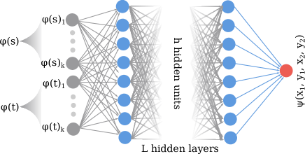
We leverage the sampling approach from the previous section to devise a learning algorithm for approximating $d_{\sim}$ and $d^{\pi}_{\sim}$ for MDPs with large (or continuous) state spaces, using function approximators in the form of neural networks. Let $\phi:\mathcal{S}\rightarrow\mathbb{R}^{k}$ be a $k$-dimensional representation of the state space and let $\psi_{\theta}:\mathbb{R}^{2k}\rightarrow\mathbb{R}$ be a neural network parameterized by $\theta$, that receives a concatenation of two state representations such that ฯˆฮธโ€‹([ฯ•โ€‹(s),ฯ•โ€‹(t)])โ‰ˆdโˆผโ€‹(s,t)subscript๐œ“๐œƒitalic-ฯ•๐‘ italic-ฯ•๐‘กsubscript๐‘‘similar-to๐‘ ๐‘ก\psi_{\theta}([\phi(s),\phi(t)])\approx d_{\sim}(s,t) (see Figureย 3).

Refer to caption
Figure 3: Using a neural network for learning $\psi$ as an approximant to $d_{\sim}$ or $d^{\pi}_{\sim}$.

Following the practice introduced by (?) we make use of online parameters $\theta$ and target parameters $\theta^{-}$, where the online parameters are updated at each iteration while the target parameters are updated every $C$ iterations. Given a pair of states sโ‰ t๐‘ ๐‘กs\neq t and action $a\in\mathcal{A}$, at iteration $i$ we define the target objective ๐“ฮธiโˆ’โ€‹(s,t,a)subscript๐“subscriptsuperscript๐œƒ๐‘–๐‘ ๐‘ก๐‘Ž\mathbf{T}_{\theta^{-}_{i}}(s,t,a) for $d_{\sim}$ as:

maxโก[|โ„›โ€‹(s,a)โˆ’โ„›โ€‹(t,a)|+ฮณโ€‹ฯˆฮธiโˆ’โ€‹([ฯ•โ€‹(๐’ฉโ€‹(s,a)),ฯ•โ€‹(๐’ฉโ€‹(t,a))]),ฯˆฮธiโˆ’โ€‹([ฯ•โ€‹(s),ฯ•โ€‹(t)])]matrixโ„›๐‘ ๐‘Žโ„›๐‘ก๐‘Ž๐›พsubscript๐œ“subscriptsuperscript๐œƒ๐‘–italic-ฯ•๐’ฉ๐‘ ๐‘Žitalic-ฯ•๐’ฉ๐‘ก๐‘Žsubscript๐œ“subscriptsuperscript๐œƒ๐‘–italic-ฯ•๐‘ italic-ฯ•๐‘ก\displaystyle\max\begin{bmatrix}|\mathcal{R}(s,a)-\mathcal{R}(t,a)|+\gamma\psi_{\theta^{-}_{i}}([\phi(\mathscr{N}(s,a)),\phi(\mathscr{N}(t,a))]),\\ \psi_{\theta^{-}_{i}}([\phi(s),\phi(t)])\end{bmatrix}

and equal to 00 whenever s=t๐‘ ๐‘กs=t. The target objective ๐“ฮธiโˆ’ฯ€โ€‹(s,t)subscriptsuperscript๐“๐œ‹subscriptsuperscript๐œƒ๐‘–๐‘ ๐‘ก\mathbf{T}^{\pi}_{\theta^{-}_{i}}(s,t) for $d^{\pi}_{\sim}$ is:

$\displaystyle|\mathcal{R}(s,\pi(s))$ $\displaystyle-\mathcal{R}(t,\pi(t))|+$
ฮณโ€‹ฯˆฮธiโˆ’ฯ€โ€‹([ฯ•โ€‹(๐’ฉโ€‹(s,ฯ€โ€‹(s))),ฯ•โ€‹(๐’ฉโ€‹(t,ฯ€โ€‹(t)))])๐›พsubscriptsuperscript๐œ“๐œ‹subscriptsuperscript๐œƒ๐‘–italic-ฯ•๐’ฉ๐‘ ๐œ‹๐‘ italic-ฯ•๐’ฉ๐‘ก๐œ‹๐‘ก\displaystyle\gamma\psi^{\pi}_{\theta^{-}_{i}}([\phi(\mathscr{N}(s,\pi(s))),\phi(\mathscr{N}(t,\pi(t)))])

We can then define our loss โ„’s,t,a(ฯ€)subscriptsuperscriptโ„’๐œ‹๐‘ ๐‘ก๐‘Ž\mathcal{L}^{(\pi)}_{s,t,a} as: ๐”ผ๐’Ÿโ€‹(๐“ฮธiโˆ’(ฯ€)โ€‹(s,t,a)โˆ’ฯˆฮธi(ฯ€)โ€‹([ฯ•โ€‹(s),ฯ•โ€‹(t)]))2subscript๐”ผ๐’Ÿsuperscriptsubscriptsuperscript๐“๐œ‹subscriptsuperscript๐œƒ๐‘–๐‘ ๐‘ก๐‘Žsubscriptsuperscript๐œ“๐œ‹subscript๐œƒ๐‘–italic-ฯ•๐‘ italic-ฯ•๐‘ก2\mathbb{E}_{\mathcal{D}}\left(\mathbf{T}^{(\pi)}_{\theta^{-}_{i}}(s,t,a)-\psi^{(\pi)}_{\theta_{i}}([\phi(s),\phi(t)])\right)^{2}. This loss is specified for a single pair of transitions, but we can define an analogous target and loss with mini-batches, which allows us to train our approximant more efficiently using specialized hardware such as GPUs:

$\displaystyle\mathbf{T}$ $\displaystyle=(1-\mathbf{I})\otimes\max\left(\mathbf{R}^{2}+\gamma\beta\psi_{\theta^{-}_{i}}(\mathbf{N}^{2}),\beta\psi_{\theta^{-}_{i}}(\mathbf{S}^{2})\right)$
$\displaystyle\mathcal{L}_{i}(\theta_{i})$ $\displaystyle=\mathbb{E}_{\mathcal{D}}\left[\mathbf{W}\otimes\left(\psi_{\theta_{i}}(\mathbf{S}^{2})-\mathbf{T}\right)^{2}\right]$
$\displaystyle\mathbf{T}^{\pi}$ $\displaystyle=(1-\mathbf{I})\left(\mathbf{R}^{2}+\gamma\beta\psi^{\pi}_{\theta^{-}_{i}}(\mathbf{N}^{2})\right)$
$\displaystyle\mathcal{L}^{\pi}_{i}(\theta_{i})$ $\displaystyle=\mathbb{E}_{\mathcal{D}}\left[\left(\psi^{\pi}_{\theta_{i}}(\mathbf{S}^{2})-\mathbf{T}\right)^{2}\right]$
Refer to caption
Figure 4: GridWorld and its (x, y) representation. Black densities illustrate the sampled states when adding noise.

$\mathbf{R}^{2}$, $\mathbf{S}^{2}$, and $\mathbf{N}^{2}$ are batches of rewards, states, and next-states, respectively, $\mathbf{W}$ is a mask used to enforce action matching when approximating $d_{\sim}$, and $\mathbf{I}$ is the identity matrix. $\psi(\mathbf{X})$ indicates applying $\psi$ to a matrix $\mathbf{X}$ elementwise, and $\otimes$ stands for the Hadamard product. We multiply by $(1-\mathbf{I})$ to zero out the diagonals, since those represent approximations to dโˆผ(ฯ€)โ€‹(s,s)โ‰ก0subscriptsuperscript๐‘‘๐œ‹similar-to๐‘ ๐‘ 0d^{(\pi)}_{\sim}(s,s)\equiv 0. The parameter $\beta$ is a stability parameter that begins at 00 and is incremented towards $1$ every $C$ iterations. Its purpose is to gradually โ€œgrowโ€ the effective horizon of the bisimulation backup and maximization. This is helpful since the approximant $\psi_{\theta}$ can have some variance initially, depending on how $\theta$ is initialized. Further, ? (?) demonstrate that using shorter horizons during planning can often be better than using the true horizon, especially when using a model estimated from data. Note that, in general, the approximant $\psi$ is not guaranteed to be a proper pseudometric. A lengthier discussion, including the derivation of these matrices, is provided in the supplemental material.

Refer to caption
(a) Absolute metric errors on the GridWorld.
Refer to caption
(b) Normalized metric errors.
Figure 5: Metric errors for the learned metric on the GridWorld as training progresses.

Empirical evaluation

In this section we provide empirical evidence for the effectiveness of our bisimulation approximants333Code available at https://github.com/google-research/google-research/tree/master/bisimulation_aaai2020. We begin with a simple 31-state GridWorld, on which we can compute the bisimulation metric exactly, and use a โ€œnoisyโ€ representation which yields a continuous-state MDP. Having the exact metric for the 31-state MDP allows us to quantitatively measure the quality of our learned approximant.

We then learn a $\pi$-bisimulation approximant over policies generated by reinforcement learning agents trained on Atari 2600 games. In the supplemental material we provide an extensive discussion of the hyperparameter search we performed to find the settings used for both experiments. Training was done on a Tesla P100 GPU.

GridWorld

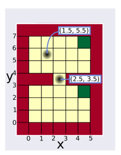
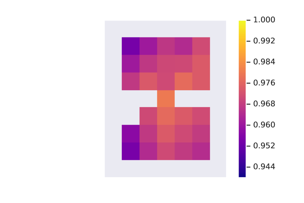
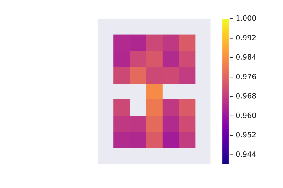
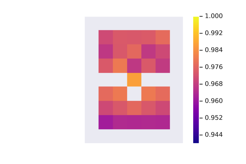
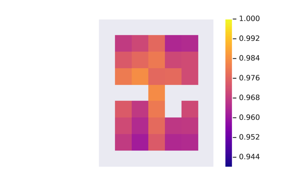
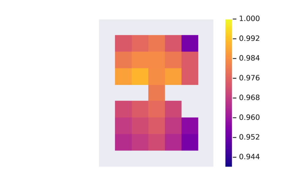
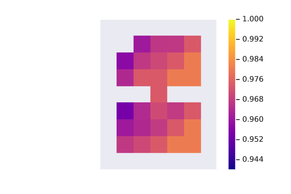
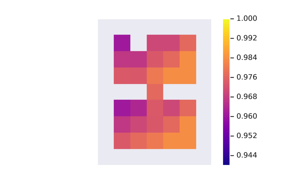
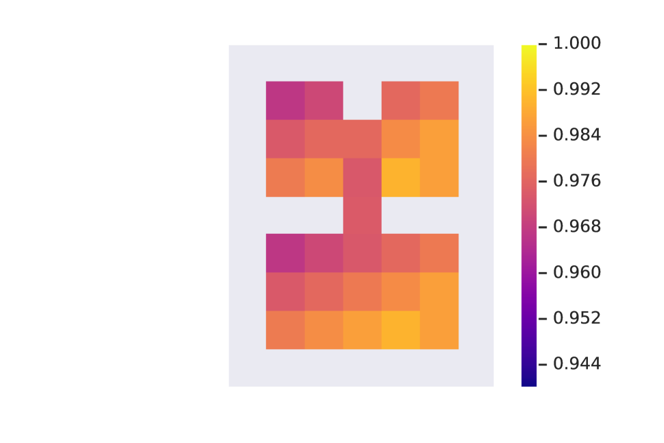
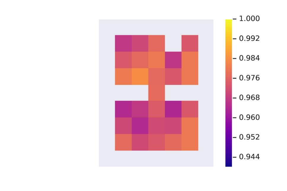
We first evaluate our learning algorithms on the 31-state GridWorld environment illustrated in Figureย 4. There are 4 actions (up, down, left, right) with deterministic transitions, and where an action driving the agent towards a wall keeps the agent in the same cell. There is a single reward of $+1.0$ received upon entering either of the green cells, and a reward of $-1.0$ for taking an action towards a wall. We display the bisimulation distances between all states in the supplemental, computed using the sampling approach.

We represent each state by its coordinates $(x,y)\in\mathbb{R}^{2}$, as illustrated in Figureย 4. To estimate $d_{\sim}$ we use a network with an input layer of dimension $4$, one fully connected hidden layer with $729$ hidden units, and an output of length $1$. The input is the concatenation of two state representations, normalized to be in $[-1,1]$, while the output value is the estimate to $d_{\sim}$. We sampled state pairs and actions uniformly randomly, and ran our experiments with $\gamma=0.99$, $C=500$, $b=256$, and increased $\beta$ from 00 to $1$ by a factor of $0.9$ every time the target network was updated; we used the Adam optimizer (?) with a learning rate of $0.01$. Because of the maximization term in the target, these networks can have a tendency to overshoot (although the combination of target networks and the $\beta$ term helps stabilize this); we ran the training process for $2500$ steps, which, for this problem, was long enough to converge to a reasonable solution before overshooting. The full hyperparameter settings are provided in the supplemental.

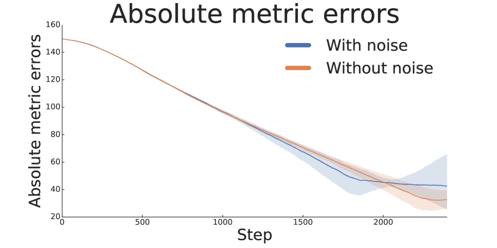
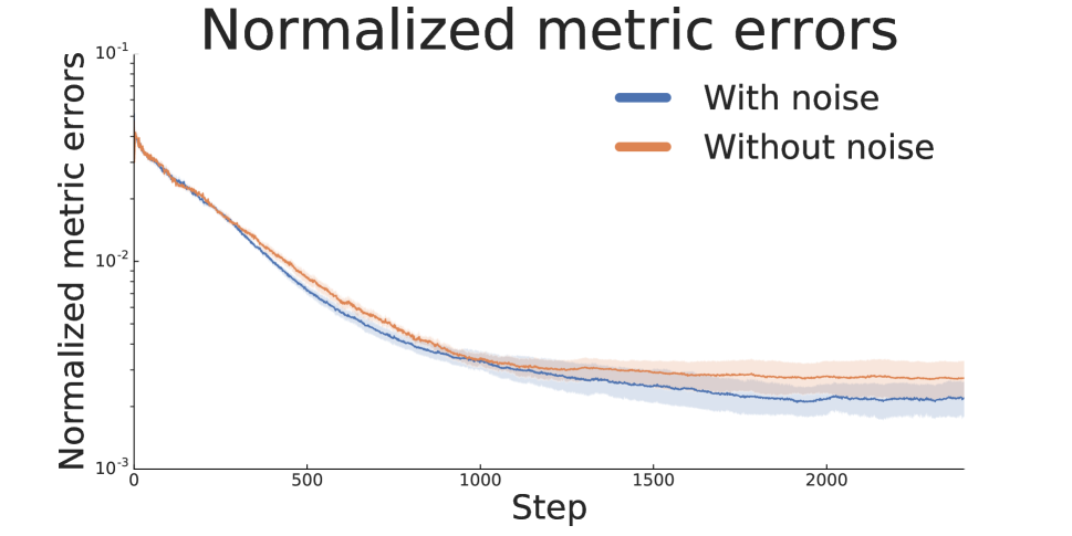
To evaluate the learning process, we measure the absolute error: $\|d_{\sim}-\psi\|_{\infty}$ using the true underlying state space for which we know the value of $d_{\sim}$. Note that because there is no fixed learning target, absolute errors are not guaranteed to be bounded. For this reason we also report the normalized error: $\|\frac{d_{\sim}}{\|d_{\sim}\|_{2}}-\frac{\psi}{\|\psi\|_{2}}\|_{\infty}$ as in practice one is mostly interested in relative, rather than absolute, distances. 5(a) and 5(b) display the results of our experiments over 10 independent runs; the shaded areas represent the 95% confidence interval.

In addition to training on the 31 state-MDP, we constructed a continuous variant by adding Gaussian noise to the state representations; this noise is centered at $(0,0)$ with standard deviation $0.1$, and clipped to be in $[-0.3,0.3]$. The per-cell noise is illustrated by the black gradients in Figureย 4. As Figureย 5 shows, there is little difference between learning the metric for the 31-state MDP versus learning it for its continuous variant. Adding noise does not seem to hurt performance, and in fact seems to be helpful. We hypotheisze that noise may be acting as a form of regularization, but this requires further investigation. In the supplemental material we include a figure exploring using the metric approximant for aggregating states in the continuous MDP setting with promising results.

Atari 2600

To evaluate the performance of our learning algorithm on an existing large problem, we take a set of reinforcement learning (RL) agents trained on three Atari 2600 games from the Arcade Learning Environment (?). The RL agents were obtained from the set of trained agents provided with the Dopamine library (?). Because our methods are designed for deterministic MDPs, we only used those trained without sticky actions444Sticky actions add stochasticity to action outcomes.ย (?) (evaluated in Sectionย 4.3 in (?)); the trained checkpoints were provided for only three games: Space Invaders, Pong, and Asterix. We used the Rainbow agent (?) as it is the best performing of the provided Dopamine agents. We used the penultimate layer of the trained Rainbow agent as the representation $\phi$.

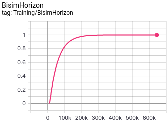
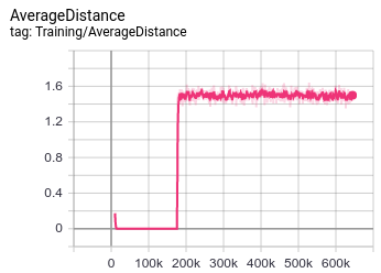
To approximate the on-policy bisimulation metric $d^{\pi}_{\sim}$ we loaded a trained agent and ran it in evaluation mode for each respective game, filling up the replay buffer while doing so. Once 10,000 transitions have been stored in the replay buffer, we begin sampling mini-batches and update our approximant $\psi^{\pi}_{\theta}$ using the target and loss defined previously. (note that we still continue populating our replay buffer). We ran our experiments using a network of two hidden layers of dimension $16$, with $\gamma=0.99$, $C=500$, $b=128$, and increased the $\beta$ term from 00 to $1$ by a factor of $0.99$ every time the target network was updated. We used the Adam optimizer (?) with a learning rate of $7.5e^{-5}$ (except for Pong where we found $0.001$ yielded better results). We trained the networks for around $600K$ steps, although in practice we found that about half that many steps were needed to reach a stable approximant. The configuration file specifying the full hyperparameter settings as well as the learning curves are provided in the supplemental.

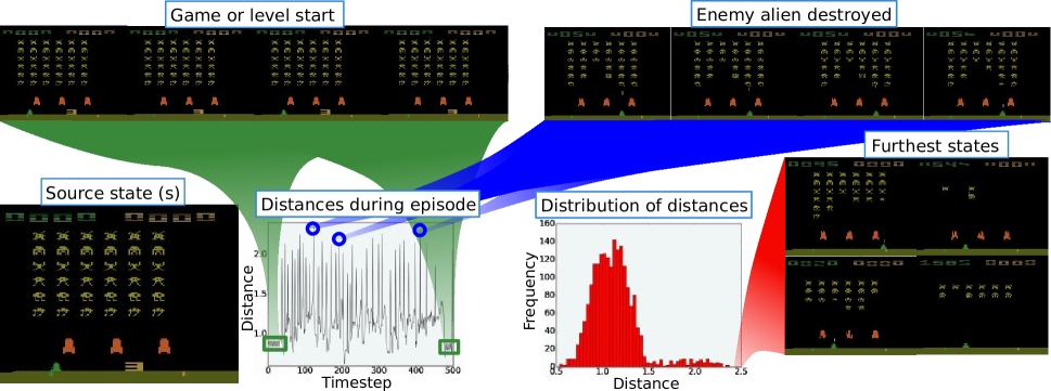
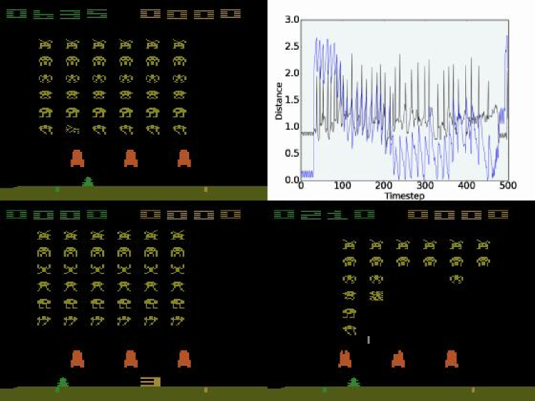
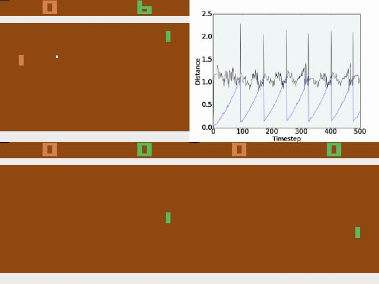
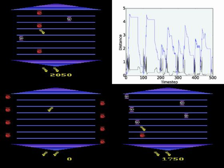
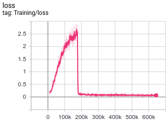
After training we evaluated our approximant ฯˆฮธฯ€โ€‹([ฯ•โ€‹(s),ฯ•โ€‹(t)])subscriptsuperscript๐œ“๐œ‹๐œƒitalic-ฯ•๐‘ italic-ฯ•๐‘ก\psi^{\pi}_{\theta}([\phi(s),\phi(t)]) by fixing s๐‘ s to be the first state in the game and varying $t$ throughout the episode; that is, we evaluate how similar the other states of the game are to the initial state w.r.t. our metric approximant. In Figureย 6 we display the first 500 steps of one evaluation run on Space Invaders; as can be seen, the learned metric captures more meaningful differences between frames (start of episodes, enemy alien destroyed) that go beyond simple pixel differences. Interestingly, when sorting the frames by distance, the frames furthest away from s๐‘ s are typically those where the agent is about to be killed. It is worth noting that the way states are encoded in Dopamine is by stacking the last four frames; in our visualization we are only displaying the top frame in this stack. We observed similar results for Asterix and Pong; we include these and more extensive results, as well as videos for the three games, in the supplemental material.

Related work

There are a number of different notions of state similarity that have been studied over the years. ? (?) provide a unified characterization and analysis of many of them. MDP-homomorphismsย (?) do not require behavioral equivalence under the same action labels, and this idea was extended to a metric by ? (?).

Refer to caption
Figure 6: Evaluating the approximant to $d^{\pi}_{\sim}$ with an eval run on Space Invaders. We plot the distance between the source state s๐‘ s (pictured in the bottom left) and every other state, highlighting the relatively low distances in game or level starts (green shading pointing to left and right side of the plot), as well as the peaks occuring when an enemy alien is destroyed (blue shading pointing to the distance peaks). On the bottom right we display the distribution of distances and the four furthest states for this run.

? (?) introduced a sampling-based approximation to $d_{\sim}$ which exchanges the computation of the Wasserstein with an instance of the assignment problem from network optimization; although ? (?) derived a PAC-bound for this approximant, the number of samples required is still prohibitive. ? (?) exploit the underlying structure in $\mathcal{S}$ to compute $d_{\sim}$.

Although there has been some work in concurrency theory to approximate large systems via โ€˜polynomially accurateโ€™ simulations (?), they make no use of function approximators in the form of neural networks. We believe our use of neural networks may grant our approach greater generalizability.

Deterministic on-policy systems can be reduced to a graph. As such, our notion of $\pi$-bisimulation metrics bears a close relationship to graph similarity measures (?). However, graph similarity notions compare two full systems (graphs), as opposed to two nodes within a single graph, as we evaluate here. Nonetheless, the relationship warrants further investigation, which we leave for future work.

Perhaps most related to our sampling method is the on-the-fly methods introduced by ? (?). The authors replace the use of standard dynamic programming in their computation with something akin to asynchronous dynamic programming (?), where not all state-pairs are updated at each iteration, but rather $\mathcal{S}$ is split into disjoint sets that are updated at different intervals. A few strategies for sampling state-pairs are discussed, of which the most similar to ours is the โ€œuniform asynchronous updateโ€.

? (?) introduced DeepMDP latent models and established a close relationship with bisimulation metrics (specifically, Theorem 4 in their paper). Although closely related, there are some important differences. Their work deals with state representations, where the distance between states is their distance in the representation space; by contrast, our proposed neural networks approximate the bisimulation metric between two states, independent of their representation. Further, the authors use the DeepMDP losses as an auxiliary task without a guarantee that their representations are consistent with their theoretical results. In our work we are able to show that our approximant is valid both quantitatively (GridWorld) and qualitatively (Atari 2600). Nonetheless, a natural extension of our work is to use the bisimulation losses we introduced as a means to learn better representations.

Conclusion

We introduced new methods for computing and approximating bisimulation metrics in large deterministic MDPs. The first is an exact method that converges to the true metric asymptotically, and the second is a differentiable method for approximating the metric which we demonstrated can learn a good approximant even in continuous state spaces. Since their introduction, bisimulation metrics have been used for theoretical analysis or in MDPs of small-to-moderate size, but they have scarcely been used in larger problems. Our results open the doors for their application in systems with a large, and even continuous, state space.

One important avenue for research is to extend these results to stochastic systems. Computing the Wasserstein metric without access to a generative model is challenging for deep RL environments, as the next-state samples typically come from single trajectories in replay buffers. One possibility is to build a model of the transition dynamics from the transitions in the replay buffer and compute the Wasserstein metrics from this estimate.

Although the network architecture and hyperparameters used to train $d^{\pi}_{\sim}$ are by no means optimal, the results we presented for the Atari 2600 domain are very promising and suggest that bisimulation metrics can be used effectively for deep reinforcement learning. Some promising areas we are currently exploring are using bisimulation metrics as an auxiliary task for improved state representation, as a mechanism for compressing replay buffers, and as a tool for more efficient exploration.

Acknowledgements

The author would like to thank Marc G. Bellemare, Gheorghe Comanici, Marlos C. Machado, Doina Precup, Carles Gelada, as well as the rest of the Google Brain team in Montreal for helpful discussions. The author would also like to thank the anonymous reviewers for their useful feedback while reviewing this work.

References

  • [2015] Abadi, M.; Agarwal, A.; Barham, P.; Brevdo, E.; Chen, Z.; Citro, C.; Corrado, G.ย S.; Davis, A.; Dean, J.; Devin, M.; Ghemawat, S.; Goodfellow, I.; Harp, A.; Irving, G.; Isard, M.; Jia, Y.; Jozefowicz, R.; Kaiser, L.; Kudlur, M.; Levenberg, J.; Manรฉ, D.; Monga, R.; Moore, S.; Murray, D.; Olah, C.; Schuster, M.; Shlens, J.; Steiner, B.; Sutskever, I.; Talwar, K.; Tucker, P.; Vanhoucke, V.; Vasudevan, V.; Viรฉgas, F.; Vinyals, O.; Warden, P.; Wattenberg, M.; Wicke, M.; Yu, Y.; and Zheng, X. 2015. TensorFlow: Large-scale machine learning on heterogeneous systems.
  • [2013a] Bacci, G.; Bacci, G.; Larsen, K.ย G.; and Mardare, R. 2013a. Computing Behavioral Distances, Compositionally. In Mathematical Foundations of Computer Science 2013.
  • [2013b] Bacci, G.; Bacci, G.; Larsen, K.ย G.; and Mardare, R. 2013b. On-the-Fly Exact Computation of Bisimilarity Distances. In Proceedings of the 19th Int. Conf. on Tools and Algorithms for the Construction and Analysis of Systems.
  • [2006] Baier, C.; Hermanns, H.; Katoen, J.; and Wolf, V. 2006. Bisimulation and simulation relations for markov chains. In Essays on Algebraic Process Calculi, numberย 10 in Electronic Notes in Theoretical Computer Science, 73โ€“78. Elsevier.
  • [2013] Bellemare, M.ย G.; Naddaf, Y.; Veness, J.; and Bowling, M. 2013. The Arcade Learning Environment: An evaluation platform for general agents. Jour. of AI Research 47:253โ€“279.
  • [1957] Bellman, R. 1957. Dynamic Programming. Princeton, NJ, USA: University Press.
  • [2010] Castro, P.ย S., and Precup, D. 2010. Using bisimulation for policy transfer in MDPs. In Proceedings of the 9th International Conference on Autonomous Agents and Multiagent Systems (AAMAS-2010).
  • [2018] Castro, P.ย S.; Moitra, S.; Gelada, C.; Kumar, S.; and Bellemare, M.ย G. 2018. Dopamine: A Research Framework for Deep Reinforcement Learning (arxiv.org/abs/1812.06110).
  • [2011] Castro, P.ย S. 2011. On planning, prediction and knowledge transfer in Fully and Partially Observable Markov Decision Processes. Ph.D. Dissertation, McGill University.
  • [2012] Chen, D.; van Breugel, F.; and Worrell, J. 2012. On the Complexity of Computing Probabilistic Bisimilarity. In Found. of Software Science and Computational Structures.
  • [2012] Comanici, G.; Panangaden, P.; and Precup, D. 2012. On-the-Fly Algorithms for Bisimulation Metrics. In Proc. of the 9th Int. Conf. on Quantitative Evaluation of Systems.
  • [1999] Desharnais, J.; Gupta, V.; Jagadeesan, R.; and Panangaden, P. 1999. Metrics for Labeled Markov Systems. In CONCURโ€™99 Concurrency Theory, 258โ€“273.
  • [2014] Ferns, N., and Precup, D. 2014. Bisimulation Metrics are Optimal Value Functions. In Proceedings of the 30th Conference on Uncertainty in Artificial Intelligence.
  • [2006] Ferns, N.; Castro, P.ย S.; Precup, D.; and Panangaden, P. 2006. Methods for computing state similarity in Markov decision processes. In Proceedings of the 22nd Conference on Uncertainty in Artificial Intelligence, UAI โ€™06.
  • [2004] Ferns, N.; Panangaden, P.; and Precup, D. 2004. Metrics for Finite Markov Decision Processes. In Proceedings of the 20th Conference on Uncertainty in Artificial Intelligence.
  • [2016] Ferrerย Fioriti, L.ย M.; Hashemi, V.; Hermanns, H.; and Turrini, A. 2016. Deciding probabilistic automata weak bisimulation: Theory and practice. Form. Asp. Comput. 28(1):109โ€“143.
  • [2019] Gelada, C.; Kumar, S.; Buckman, J.; Nachum, O.; and Bellemare, M.ย G. 2019. DeepMDP: Learning Continuous Latent Space Models for Representation Learning. In Proceedings of the 36th International Conference on Machine Learning.
  • [2003] Givan, R.; Dean, T.; and Greig, M. 2003. Equivalence notions and model minimization in Markov decision processes. Artificial Intelligence 147:163โ€“223.
  • [2018] Hessel, M.; Modayil, J.; van Hasselt, H.; Schaul, T.; Ostrovski, G.; Dabney, W.; Horgan, D.; Piot, B.; Azar, M.; and Silver, D. 2018. Rainbow: Combining Improvements in Deep Reinforcement learning. In Proceedings of the AAAI Conference on Artificial Intelligence.
  • [2015] Jiang, N.; Kulesza, A.; Singh, S.; and Lewis, R. 2015. The Dependence of Effective Planning Horizon on Model Accuracy. In Proceedings of the 14th International Conference on Autonomous Agents and Multiagent Systems (AAMAS-15).
  • [2007] Katoen, J.-P.; Kemna, T.; Zapreev, I.; and Jansen, D.ย N. 2007. Bisimulation minimisation mostly speeds up probabilistic model checking. In Tools and Algorithms for the Construction and Analysis of Systems, 87โ€“101.
  • [2015] Kingma, D.ย P., and Ba, J. 2015. Adam: A method for stochastic optimization. In Proceedings of the International Conference on Learning Representations.
  • [2006] Li, L.; Walsh, T.ย J.; and Littman, M.ย L. 2006. Towards a unified theory of state abstraction for mdps. In Proceedings of the Ninth International Symposium on Artificial Intelligence and Mathematics, 531โ€“539.
  • [2018] Machado, M.ย C.; Bellemare, M.ย G.; Talvitie, E.; Veness, J.; Hausknecht, M.; and Bowling, M. 2018. Revisiting the Arcade Learning Environment: Evaluation protocols and open problems for general agents. Journal of AI Research.
  • [2015] Mnih, V.; Kavukcuoglu, K.; Silver, D.; Rusu, A.ย A.; Veness, J.; Bellemare, M.ย G.; Graves, A.; Riedmiller, M.; Fidjeland, A.ย K.; Ostrovski, G.; Petersen, S.; Beattie, C.; Sadik, A.; Antonoglou, I.; King, H.; Kumaran, D.; Wierstra, D.; Legg, S.; and Hassabis, D. 2015. Human-level control through deep reinforcement learning. Nature.
  • [1994] Puterman, M.ย L. 1994. Markov Decision Processes: Discrete Stochastic Dynamic Programming. New York, NY, USA: John Wiley & Sons, Inc., 1st edition.
  • [2003] Ravindran, B., and Barto, A.ย G. 2003. Relativized Options: Choosing the Right Transformation. In Proceedings of the 20th International Conference on Machine Learning.
  • [2015] Ruan, S.; Comanici, G.; Panangaden, P.; and Precup, D. 2015. Representation discovery for mdps using bisimulation metrics. In AAAI Conference on Artificial Intelligence.
  • [2011] Sangiorgi, D. 2011. Introduction to Bisimulation and Coinduction. Cambridge University Press.
  • [2019] Santara, A.; Madan, R.; Ravindran, B.; and Mitra, P. 2019. Extra: Transfer-guided exploration. CoRR abs/1906.11785.
  • [2007] Segala, R., and Turrini, A. 2007. Approximated computationally bounded simulation relations for probabilistic automata. In Proceedings of the 20th IEEE Computer Security Foundations Symposium (CSFโ€™07).
  • [1998] Sutton, R.ย S., and Barto, A.ย G. 1998. Introduction to Reinforcement Learning. Cambridge, MA, USA: MIT Press.
  • [2009] Taylor, J.; Precup, D.; and Panagaden, P. 2009. Bounding Performance Loss in Approximate MDP Homomorphisms. In Advances in Neural Information Processing Systems 21. 1649โ€“1656.
  • [2008] Villani, C. 2008. Optimal Transport. Springer-Verlag Berlin Heidelberg.
  • [2008] Zager, L.ย A., and Verghese, G.ย C. 2008. Graph similarity scoring and matching. Applied Mathematics Letters 21(1):86 โ€“ 94.

Appendix A Proofs of the theoretical results

See 2

Proof.

This proof mimics the proof of Theoremย 4.5 from (?) (included as Theoremย 1 in this paper). Lemmaย 4.1 from that paper holds under Definitionย 3 by definition. We make use of the same pointwise ordering on $\mathcal{M}$: $d\leq d^{\prime}$ iff dโ€‹(s,t)โ‰คdโ€ฒโ€‹(s,t)๐‘‘๐‘ ๐‘กsuperscript๐‘‘โ€ฒ๐‘ ๐‘กd(s,t)\leq d^{\prime}(s,t) for all s,tโˆˆ๐’ฎ๐‘ ๐‘ก๐’ฎs,t\in\mathcal{S}, which gives us an $\omega$-cpo with bottom $\bot$, which is the everywhere-zero metric. Since Lemmaย 4.4 from (?) ($\mathcal{W}$ is continuous) also applies in our definition, it only remains to show that $\mathcal{F}^{\pi}$ is continuous:

โ„ฑฯ€โ€‹(โจ†nโˆˆโ„•{xn})โ€‹(s,t)superscriptโ„ฑ๐œ‹subscriptsquare-union๐‘›โ„•subscript๐‘ฅ๐‘›๐‘ ๐‘ก\displaystyle\mathcal{F}^{\pi}(\bigsqcup_{n\in\mathbb{N}}\{x_{n}\})(s,t) =|โ„›sฯ€โˆ’โ„›tฯ€|+ฮณโ€‹๐’ฒโ€‹(โจ†nโˆˆโ„•{xn})โ€‹(๐’ซsฯ€,๐’ซtฯ€)absentsubscriptsuperscriptโ„›๐œ‹๐‘ subscriptsuperscriptโ„›๐œ‹๐‘ก๐›พ๐’ฒsubscriptsquare-union๐‘›โ„•subscript๐‘ฅ๐‘›subscriptsuperscript๐’ซ๐œ‹๐‘ subscriptsuperscript๐’ซ๐œ‹๐‘ก\displaystyle=|\mathcal{R}^{\pi}_{s}-\mathcal{R}^{\pi}_{t}|+\gamma\mathcal{W}\left(\bigsqcup_{n\in\mathbb{N}}\{x_{n}\}\right)(\mathcal{P}^{\pi}_{s},\mathcal{P}^{\pi}_{t})
=|โ„›sฯ€โˆ’โ„›tฯ€|+ฮณโ€‹supnโˆˆโ„•๐’ฒโ€‹(xn)โ€‹(๐’ซsฯ€,๐’ซtฯ€)by continuity ofย โ€‹๐’ฒabsentsubscriptsuperscriptโ„›๐œ‹๐‘ subscriptsuperscriptโ„›๐œ‹๐‘ก๐›พsubscriptsupremum๐‘›โ„•๐’ฒsubscript๐‘ฅ๐‘›subscriptsuperscript๐’ซ๐œ‹๐‘ subscriptsuperscript๐’ซ๐œ‹๐‘กby continuity ofย ๐’ฒ\displaystyle=|\mathcal{R}^{\pi}_{s}-\mathcal{R}^{\pi}_{t}|+\gamma\sup_{n\in\mathbb{N}}\mathcal{W}(x_{n})(\mathcal{P}^{\pi}_{s},\mathcal{P}^{\pi}_{t})\quad\textrm{by continuity of }\mathcal{W}
=supnโˆˆโ„•(|โ„›sฯ€โˆ’โ„›tฯ€|+ฮณโ€‹๐’ฒโ€‹(xn)โ€‹(๐’ซsฯ€,๐’ซtฯ€))absentsubscriptsupremum๐‘›โ„•subscriptsuperscriptโ„›๐œ‹๐‘ subscriptsuperscriptโ„›๐œ‹๐‘ก๐›พ๐’ฒsubscript๐‘ฅ๐‘›subscriptsuperscript๐’ซ๐œ‹๐‘ subscriptsuperscript๐’ซ๐œ‹๐‘ก\displaystyle=\sup_{n\in\mathbb{N}}\left(|\mathcal{R}^{\pi}_{s}-\mathcal{R}^{\pi}_{t}|+\gamma\mathcal{W}(x_{n})(\mathcal{P}^{\pi}_{s},\mathcal{P}^{\pi}_{t})\right)
=supnโˆˆโ„•{โ„ฑฯ€โ€‹(xn)โ€‹(s,t)}absentsubscriptsupremum๐‘›โ„•superscriptโ„ฑ๐œ‹subscript๐‘ฅ๐‘›๐‘ ๐‘ก\displaystyle=\sup_{n\in\mathbb{N}}\left\{\mathcal{F}^{\pi}(x_{n})(s,t)\right\}
=(โจ†nโˆˆโ„•{โ„ฑฯ€โ€‹(xn)})โ€‹(s,t)absentsubscriptsquare-union๐‘›โ„•superscriptโ„ฑ๐œ‹subscript๐‘ฅ๐‘›๐‘ ๐‘ก\displaystyle=\left(\bigsqcup_{n\in\mathbb{N}}\left\{\mathcal{F}^{\pi}(x_{n})\right\}\right)(s,t)

The rest of the proof follows in the same way as in (?). โˆŽ

See 3

Proof.

We will use the standard value function update: Vnฯ€โ€‹(s)=โ„›sฯ€+ฮณโ€‹โˆ‘sโ€ฒโˆˆ๐’ฎ๐’ซsฯ€โ€‹(sโ€ฒ)โ€‹Vnโˆ’1ฯ€โ€‹(sโ€ฒ)subscriptsuperscript๐‘‰๐œ‹๐‘›๐‘ subscriptsuperscriptโ„›๐œ‹๐‘ ๐›พsubscriptsuperscript๐‘ โ€ฒ๐’ฎsubscriptsuperscript๐’ซ๐œ‹๐‘ superscript๐‘ โ€ฒsubscriptsuperscript๐‘‰๐œ‹๐‘›1superscript๐‘ โ€ฒV^{\pi}_{n}(s)=\mathcal{R}^{\pi}_{s}+\gamma\sum_{s^{\prime}\in\mathcal{S}}\mathcal{P}^{\pi}_{s}(s^{\prime})V^{\pi}_{n-1}(s^{\prime}) with $V^{\pi}_{0}\equiv 0$ and our update operator from Theoremย 2: dnฯ€โ€‹(s,t)=โ„ฑฯ€โ€‹(dnโˆ’1ฯ€)โ€‹(s,t)subscriptsuperscript๐‘‘๐œ‹๐‘›๐‘ ๐‘กsuperscriptโ„ฑ๐œ‹subscriptsuperscript๐‘‘๐œ‹๐‘›1๐‘ ๐‘กd^{\pi}_{n}(s,t)=\mathcal{F}^{\pi}(d^{\pi}_{n-1})(s,t) with $d^{\pi}_{0}\equiv 0$, and prove this by induction, showing that for all $n\in\mathbb{N}$ and s,tโˆˆ๐’ฎ๐‘ ๐‘ก๐’ฎs,t\in\mathcal{S}, |Vnฯ€โ€‹(s)โˆ’Vnฯ€โ€‹(t)|โ‰คdnฯ€โ€‹(s,t)subscriptsuperscript๐‘‰๐œ‹๐‘›๐‘ subscriptsuperscript๐‘‰๐œ‹๐‘›๐‘กsubscriptsuperscript๐‘‘๐œ‹๐‘›๐‘ ๐‘ก|V^{\pi}_{n}(s)-V^{\pi}_{n}(t)|\leq d^{\pi}_{n}(s,t).

The base case holds vacuously: 0=V0ฯ€โ€‹(s,t)โ‰คd0ฯ€โ€‹(s,t)=00subscriptsuperscript๐‘‰๐œ‹0๐‘ ๐‘กsubscriptsuperscript๐‘‘๐œ‹0๐‘ ๐‘ก00=V^{\pi}_{0}(s,t)\leq d^{\pi}_{0}(s,t)=0, so assume true up to $n$.

|Vn+1ฯ€โ€‹(s)โˆ’Vn+1ฯ€โ€‹(t)|subscriptsuperscript๐‘‰๐œ‹๐‘›1๐‘ subscriptsuperscript๐‘‰๐œ‹๐‘›1๐‘ก\displaystyle|V^{\pi}_{n+1}(s)-V^{\pi}_{n+1}(t)| =|โ„›sฯ€+ฮณโ€‹โˆ‘sโ€ฒโˆˆ๐’ฎ๐’ซsฯ€โ€‹(sโ€ฒ)โ€‹Vnฯ€โ€‹(sโ€ฒ)โˆ’(โ„›tฯ€+ฮณโ€‹โˆ‘sโ€ฒโˆˆ๐’ฎ๐’ซtฯ€โ€‹(sโ€ฒ)โ€‹Vnฯ€โ€‹(sโ€ฒ))|absentsubscriptsuperscriptโ„›๐œ‹๐‘ ๐›พsubscriptsuperscript๐‘ โ€ฒ๐’ฎsubscriptsuperscript๐’ซ๐œ‹๐‘ superscript๐‘ โ€ฒsubscriptsuperscript๐‘‰๐œ‹๐‘›superscript๐‘ โ€ฒsubscriptsuperscriptโ„›๐œ‹๐‘ก๐›พsubscriptsuperscript๐‘ โ€ฒ๐’ฎsubscriptsuperscript๐’ซ๐œ‹๐‘กsuperscript๐‘ โ€ฒsubscriptsuperscript๐‘‰๐œ‹๐‘›superscript๐‘ โ€ฒ\displaystyle=\left|\mathcal{R}^{\pi}_{s}+\gamma\sum_{s^{\prime}\in\mathcal{S}}\mathcal{P}^{\pi}_{s}(s^{\prime})V^{\pi}_{n}(s^{\prime})-\left(\mathcal{R}^{\pi}_{t}+\gamma\sum_{s^{\prime}\in\mathcal{S}}\mathcal{P}^{\pi}_{t}(s^{\prime})V^{\pi}_{n}(s^{\prime})\right)\right|
โ‰ค|โ„›sฯ€โˆ’โ„›tฯ€|+|ฮณโ€‹โˆ‘sโ€ฒโˆˆ๐’ฎVnฯ€โ€‹(sโ€ฒ)โ€‹(๐’ซsฯ€โ€‹(sโ€ฒ)โˆ’๐’ซtฯ€โ€‹(sโ€ฒ))|absentsubscriptsuperscriptโ„›๐œ‹๐‘ subscriptsuperscriptโ„›๐œ‹๐‘ก๐›พsubscriptsuperscript๐‘ โ€ฒ๐’ฎsubscriptsuperscript๐‘‰๐œ‹๐‘›superscript๐‘ โ€ฒsubscriptsuperscript๐’ซ๐œ‹๐‘ superscript๐‘ โ€ฒsubscriptsuperscript๐’ซ๐œ‹๐‘กsuperscript๐‘ โ€ฒ\displaystyle\leq|\mathcal{R}^{\pi}_{s}-\mathcal{R}^{\pi}_{t}|+\left|\gamma\sum_{s^{\prime}\in\mathcal{S}}V^{\pi}_{n}(s^{\prime})(\mathcal{P}^{\pi}_{s}(s^{\prime})-\mathcal{P}^{\pi}_{t}(s^{\prime}))\right|
โ‰ค|โ„›sฯ€โˆ’โ„›tฯ€|+|ฮณโ€‹๐’ฒโ€‹(dnฯ€)โ€‹(๐’ซsฯ€,๐’ซtฯ€)|absentsubscriptsuperscriptโ„›๐œ‹๐‘ subscriptsuperscriptโ„›๐œ‹๐‘ก๐›พ๐’ฒsubscriptsuperscript๐‘‘๐œ‹๐‘›subscriptsuperscript๐’ซ๐œ‹๐‘ subscriptsuperscript๐’ซ๐œ‹๐‘ก\displaystyle\leq|\mathcal{R}^{\pi}_{s}-\mathcal{R}^{\pi}_{t}|+\left|\gamma\mathcal{W}(d^{\pi}_{n})(\mathcal{P}^{\pi}_{s},\mathcal{P}^{\pi}_{t})\right|
=|โ„›sฯ€โˆ’โ„›tฯ€|+ฮณโ€‹๐’ฒโ€‹(dnฯ€)โ€‹(๐’ซsฯ€,๐’ซtฯ€)sinceย ๐’ฒโ€‹(dnฯ€)ย is a metricabsentsubscriptsuperscriptโ„›๐œ‹๐‘ subscriptsuperscriptโ„›๐œ‹๐‘ก๐›พ๐’ฒsubscriptsuperscript๐‘‘๐œ‹๐‘›subscriptsuperscript๐’ซ๐œ‹๐‘ subscriptsuperscript๐’ซ๐œ‹๐‘กsinceย ๐’ฒ(dnฯ€)ย is a metric\displaystyle=|\mathcal{R}^{\pi}_{s}-\mathcal{R}^{\pi}_{t}|+\gamma\mathcal{W}(d^{\pi}_{n})(\mathcal{P}^{\pi}_{s},\mathcal{P}^{\pi}_{t})\quad\textrm{since $\mathcal{W}(d^{\pi}_{n})$ is a metric}
=โ„ฑฯ€โ€‹(dnฯ€)โ€‹(s,t)absentsuperscriptโ„ฑ๐œ‹subscriptsuperscript๐‘‘๐œ‹๐‘›๐‘ ๐‘ก\displaystyle=\mathcal{F}^{\pi}(d^{\pi}_{n})(s,t)
=dn+1ฯ€โ€‹(s,t)absentsubscriptsuperscript๐‘‘๐œ‹๐‘›1๐‘ ๐‘ก\displaystyle=d^{\pi}_{n+1}(s,t)

where the second inequality follows from noticing that, by induction, for all s,tโˆˆ๐’ฎ๐‘ ๐‘ก๐’ฎs,t\in\mathcal{S}, Vnฯ€โ€‹(s)โˆ’Vnฯ€โ€‹(t)โ‰คdnโ€‹(s,t)subscriptsuperscript๐‘‰๐œ‹๐‘›๐‘ subscriptsuperscript๐‘‰๐œ‹๐‘›๐‘กsubscript๐‘‘๐‘›๐‘ ๐‘กV^{\pi}_{n}(s)-V^{\pi}_{n}(t)\leq d_{n}(s,t), which means $V^{\pi}$ is a feasible solution to the primal LP objective of ๐’ฒโ€‹(dnฯ€)โ€‹(๐’ซsฯ€,๐’ซtฯ€)๐’ฒsubscriptsuperscript๐‘‘๐œ‹๐‘›subscriptsuperscript๐’ซ๐œ‹๐‘ subscriptsuperscript๐’ซ๐œ‹๐‘ก\mathcal{W}(d^{\pi}_{n})(\mathcal{P}^{\pi}_{s},\mathcal{P}^{\pi}_{t}) (see Equationย 1). โˆŽ

See 1

Proof.

The primal LP defined in Equationย 1 can be expressed in its dual form (which, incidentally, is a minimum-cost flow problem):

min๐€โ€‹โˆ‘sโ€ฒ,tโ€ฒโˆˆ๐’ฎฮปsโ€ฒ,tโ€ฒโ€‹dโ€‹(sโ€ฒ,tโ€ฒ)subscript๐€subscriptsuperscript๐‘ โ€ฒsuperscript๐‘กโ€ฒ๐’ฎsubscript๐œ†superscript๐‘ โ€ฒsuperscript๐‘กโ€ฒ๐‘‘superscript๐‘ โ€ฒsuperscript๐‘กโ€ฒ\displaystyle\min_{\bm{\lambda}}\sum_{s^{\prime},t^{\prime}\in\mathcal{S}}\lambda_{s^{\prime},t^{\prime}}d(s^{\prime},t^{\prime})
s.t. โˆ€sโ€ฒโˆˆ๐’ฎ,โˆ‘tโ€ฒฮปsโ€ฒ,tโ€ฒ=๐’ซโ€‹(s,a)โ€‹(sโ€ฒ)formulae-sequencefor-allsuperscript๐‘ โ€ฒ๐’ฎsubscriptsuperscript๐‘กโ€ฒsubscript๐œ†superscript๐‘ โ€ฒsuperscript๐‘กโ€ฒ๐’ซ๐‘ ๐‘Žsuperscript๐‘ โ€ฒ\displaystyle\forall s^{\prime}\in\mathcal{S},\quad\sum_{t^{\prime}}\lambda_{s^{\prime},t^{\prime}}=\mathcal{P}(s,a)(s^{\prime})
โˆ€tโ€ฒโˆˆ๐’ฎ,โˆ‘sโ€ฒฮปsโ€ฒ,tโ€ฒ=๐’ซโ€‹(t,a)โ€‹(tโ€ฒ)formulae-sequencefor-allsuperscript๐‘กโ€ฒ๐’ฎsubscriptsuperscript๐‘ โ€ฒsubscript๐œ†superscript๐‘ โ€ฒsuperscript๐‘กโ€ฒ๐’ซ๐‘ก๐‘Žsuperscript๐‘กโ€ฒ\displaystyle\forall t^{\prime}\in\mathcal{S},\quad\sum_{s^{\prime}}\lambda_{s^{\prime},t^{\prime}}=\mathcal{P}(t,a)(t^{\prime})
$\displaystyle\bm{\lambda}\geq 0$

By the deterministic assumption it follows that ฮปsโ€ฒ,tโ€ฒ=0subscript๐œ†superscript๐‘ โ€ฒsuperscript๐‘กโ€ฒ0\lambda_{s^{\prime},t^{\prime}}=0 whenever sโ€ฒโ‰ ๐’ฉโ€‹(s,a)superscript๐‘ โ€ฒ๐’ฉ๐‘ ๐‘Žs^{\prime}\neq\mathscr{N}(s,a) or tโ€ฒโ‰ ๐’ฉโ€‹(t,a)superscript๐‘กโ€ฒ๐’ฉ๐‘ก๐‘Žt^{\prime}\neq\mathscr{N}(t,a) (since otherwise one of the first two constraints will be violated). This means that only ฮป๐’ฉโ€‹(s,a),๐’ฉโ€‹(t,a)subscript๐œ†๐’ฉ๐‘ ๐‘Ž๐’ฉ๐‘ก๐‘Ž\lambda_{\mathscr{N}(s,a),\mathscr{N}(t,a)} is positive. By the equality constraints it then follows that ฮป๐’ฉโ€‹(s,a),๐’ฉโ€‹(t,a)=1subscript๐œ†๐’ฉ๐‘ ๐‘Ž๐’ฉ๐‘ก๐‘Ž1\lambda_{\mathscr{N}(s,a),\mathscr{N}(t,a)}=1, resulting in dโ€‹(๐’ฉโ€‹(s,a),๐’ฉโ€‹(t,a))๐‘‘๐’ฉ๐‘ ๐‘Ž๐’ฉ๐‘ก๐‘Žd(\mathscr{N}(s,a),\mathscr{N}(t,a)) as the minimal objective value. โˆŽ

Lemma 2.

(Maximizing action) If $d_{0}\equiv 0$ and subsequent $d_{n}$ are udpated as in Equationย 3, then for all s,tโˆˆ๐’ฎ๐‘ ๐‘ก๐’ฎs,t\in\mathcal{S} and $\delta\in\mathbb{R}$ there exists an $n<\infty$ and $a\in\mathcal{A}$ such that
Pโ€‹rโ€‹(dnโ€‹(s,t)=|โ„›โ€‹(s,a)โˆ’โ„›โ€‹(t,a)|+ฮณโ€‹dnโˆ’1โ€‹(๐’ฉโ€‹(s,a),๐’ฉโ€‹(t,a)))>1โˆ’ฮด๐‘ƒ๐‘Ÿsubscript๐‘‘๐‘›๐‘ ๐‘กโ„›๐‘ ๐‘Žโ„›๐‘ก๐‘Ž๐›พsubscript๐‘‘๐‘›1๐’ฉ๐‘ ๐‘Ž๐’ฉ๐‘ก๐‘Ž1๐›ฟPr(d_{n}(s,t)=|\mathcal{R}(s,a)-\mathcal{R}(t,a)|+\gamma d_{n-1}(\mathscr{N}(s,a),\mathscr{N}(t,a)))>1-\delta.

Proof.

Since we start at $d_{0}\equiv 0$, the result will hold as long as we can guarantee that ฯ„s,t,asubscript๐œ๐‘ ๐‘ก๐‘Ž\tau_{s,t,a} for some $a\in\mathcal{A}$ will be sampled at least once. By assumption ๐’Ÿโ€‹(ฯ„s,t,a)>0๐’Ÿsubscript๐œ๐‘ ๐‘ก๐‘Ž0\mathcal{D}(\tau_{s,t,a})>0, which means that the probability that ฯ„s,t,asubscript๐œ๐‘ ๐‘ก๐‘Ž\tau_{s,t,a} is not sampled by step $n$ is (1โˆ’๐’Ÿโ€‹(ฯ„s,t,a))nsuperscript1๐’Ÿsubscript๐œ๐‘ ๐‘ก๐‘Ž๐‘›(1-\mathcal{D}(\tau_{s,t,a}))^{n}. We obtain our result by taking n>lnโกฮดlnโก(1โˆ’๐’Ÿโ€‹(ฯ„s,t,a))๐‘›๐›ฟ1๐’Ÿsubscript๐œ๐‘ ๐‘ก๐‘Žn>\frac{\ln\delta}{\ln(1-\mathcal{D}(\tau_{s,t,a}))}. โˆŽ

Lemma 3.

(Monotonicity) If $d_{0}\equiv 0$ and subsequent $d_{n}$ are udpated as in Equationย 3, then $d_{n}\leq d_{\sim}$ for all $n\in\mathbb{N}$.

Proof.

Obviously $d_{n-1}\leq d_{n}$ for all $n$. We will show by induction that $d_{n}\leq d_{\sim}$ for all $n$. The base case $d_{0}\equiv 0\leq d_{\sim}$ follows by definition, so assume true up to $n$ and consider any s,tโˆˆ๐’ฎ๐‘ ๐‘ก๐’ฎs,t\in\mathcal{S}, where $n$ is large enough so that we have a high likelihood of sampling ฯ„s,t,asubscript๐œ๐‘ ๐‘ก๐‘Ž\tau_{s,t,a} for some $a\in\mathcal{A}$ (from 2). First note that this implies that for all $n^{\prime}>n$ there exists an $a^{*}_{n^{\prime}}\in\mathcal{A}$ such that dnโ€ฒโ€‹(s,t)=|โ„›โ€‹(s,anโ€ฒโˆ—)โˆ’โ„›โ€‹(t,anโ€ฒโˆ—)|+ฮณโ€‹dnโ€ฒโˆ’1โ€‹(๐’ฉโ€‹(s,anโ€ฒโˆ—),๐’ฉโ€‹(t,anโ€ฒโˆ—))subscript๐‘‘superscript๐‘›โ€ฒ๐‘ ๐‘กโ„›๐‘ subscriptsuperscript๐‘Žsuperscript๐‘›โ€ฒโ„›๐‘กsubscriptsuperscript๐‘Žsuperscript๐‘›โ€ฒ๐›พsubscript๐‘‘superscript๐‘›โ€ฒ1๐’ฉ๐‘ subscriptsuperscript๐‘Žsuperscript๐‘›โ€ฒ๐’ฉ๐‘กsubscriptsuperscript๐‘Žsuperscript๐‘›โ€ฒd_{n^{\prime}}(s,t)=|\mathcal{R}(s,a^{*}_{n^{\prime}})-\mathcal{R}(t,a^{*}_{n^{\prime}})|+\gamma d_{n^{\prime}-1}(\mathscr{N}(s,a^{*}_{n^{\prime}}),\mathscr{N}(t,a^{*}_{n^{\prime}})).

Define aโˆผโˆ—=argโกmaxaโˆˆ๐’œโก(|โ„›โ€‹(s,a)โˆ’โ„›โ€‹(t,a)|+ฮณโ€‹dโˆผโ€‹(๐’ฉโ€‹(s,a),๐’ฉโ€‹(t,a)))subscriptsuperscript๐‘Žsimilar-tosubscript๐‘Ž๐’œโ„›๐‘ ๐‘Žโ„›๐‘ก๐‘Ž๐›พsubscript๐‘‘similar-to๐’ฉ๐‘ ๐‘Ž๐’ฉ๐‘ก๐‘Ža^{*}_{\sim}=\arg\max_{a\in\mathcal{A}}\left(|\mathcal{R}(s,a)-\mathcal{R}(t,a)|+\gamma d_{\sim}(\mathscr{N}(s,a),\mathscr{N}(t,a))\right). We then have:

dโˆผโ€‹(s,t)subscript๐‘‘similar-to๐‘ ๐‘ก\displaystyle d_{\sim}(s,t) =|โ„›โ€‹(s,aโˆผโˆ—)โˆ’โ„›โ€‹(t,aโˆผโˆ—)|+ฮณโ€‹dโˆผโ€‹(๐’ฉโ€‹(s,aโˆผโˆ—),๐’ฉโ€‹(t,aโˆผโˆ—))absentโ„›๐‘ subscriptsuperscript๐‘Žsimilar-toโ„›๐‘กsubscriptsuperscript๐‘Žsimilar-to๐›พsubscript๐‘‘similar-to๐’ฉ๐‘ subscriptsuperscript๐‘Žsimilar-to๐’ฉ๐‘กsubscriptsuperscript๐‘Žsimilar-to\displaystyle=|\mathcal{R}(s,a^{*}_{\sim})-\mathcal{R}(t,a^{*}_{\sim})|+\gamma d_{\sim}(\mathscr{N}(s,a^{*}_{\sim}),\mathscr{N}(t,a^{*}_{\sim}))
โ‰ฅ|โ„›โ€‹(s,anโˆ—)โˆ’โ„›โ€‹(t,anโˆ—)|+ฮณโ€‹dโˆผโ€‹(๐’ฉโ€‹(s,anโˆ—),๐’ฉโ€‹(t,anโˆ—))absentโ„›๐‘ subscriptsuperscript๐‘Ž๐‘›โ„›๐‘กsubscriptsuperscript๐‘Ž๐‘›๐›พsubscript๐‘‘similar-to๐’ฉ๐‘ subscriptsuperscript๐‘Ž๐‘›๐’ฉ๐‘กsubscriptsuperscript๐‘Ž๐‘›\displaystyle\geq|\mathcal{R}(s,a^{*}_{n})-\mathcal{R}(t,a^{*}_{n})|+\gamma d_{\sim}(\mathscr{N}(s,a^{*}_{n}),\mathscr{N}(t,a^{*}_{n}))
โ‰ฅ|โ„›โ€‹(s,anโˆ—)โˆ’โ„›โ€‹(t,anโˆ—)|+ฮณโ€‹dnโ€‹(๐’ฉโ€‹(s,anโˆ—),๐’ฉโ€‹(t,anโˆ—))absentโ„›๐‘ subscriptsuperscript๐‘Ž๐‘›โ„›๐‘กsubscriptsuperscript๐‘Ž๐‘›๐›พsubscript๐‘‘๐‘›๐’ฉ๐‘ subscriptsuperscript๐‘Ž๐‘›๐’ฉ๐‘กsubscriptsuperscript๐‘Ž๐‘›\displaystyle\geq|\mathcal{R}(s,a^{*}_{n})-\mathcal{R}(t,a^{*}_{n})|+\gamma d_{n}(\mathscr{N}(s,a^{*}_{n}),\mathscr{N}(t,a^{*}_{n}))
=dn+1โ€‹(s,t)absentsubscript๐‘‘๐‘›1๐‘ ๐‘ก\displaystyle=d_{n+1}(s,t)

where the second line follows from the fact that $a^{*}_{\sim}$ is the action that maximizes the bisimulation distance, and the third line follows from the inductive hypothesis. โˆŽ

See 4

Proof.

To prove this we will look at the difference
โ€–dโˆผโˆ’dnโ€–โˆž=maxs,tโˆˆ๐’ฎโก|dโˆผโ€‹(s,t)โˆ’dnโ€‹(s,t)|subscriptnormsubscript๐‘‘similar-tosubscript๐‘‘๐‘›subscript๐‘ ๐‘ก๐’ฎsubscript๐‘‘similar-to๐‘ ๐‘กsubscript๐‘‘๐‘›๐‘ ๐‘ก\|d_{\sim}-d_{n}\|_{\infty}=\max_{s,t\in\mathcal{S}}|d_{\sim}(s,t)-d_{n}(s,t)|. For any $\delta\in\mathbb{R}$ define nโˆ—=maxs,tโˆˆ๐’ฎ,aโˆˆ๐’œโก(lnโกฮดlnโก(1โˆ’๐’Ÿโ€‹(ฯ„s,t,a)))superscript๐‘›subscriptformulae-sequence๐‘ ๐‘ก๐’ฎ๐‘Ž๐’œ๐›ฟ1๐’Ÿsubscript๐œ๐‘ ๐‘ก๐‘Žn^{*}=\max_{s,t\in\mathcal{S},a\in\mathcal{A}}\left(\frac{\ln\delta}{\ln(1-\mathcal{D}(\tau_{s,t,a}))}\right). For some $n>n^{*}$, let s,t๐‘ ๐‘กs,t be the state-pair that maximizes $\|d_{\sim}-d_{n}\|_{\infty}$ at time $n$.

$\displaystyle\|d_{\sim}-d_{n}\|_{\infty}=$ |dโˆผโ€‹(s,t)โˆ’dnโ€‹(s,t)|subscript๐‘‘similar-to๐‘ ๐‘กsubscript๐‘‘๐‘›๐‘ ๐‘ก\displaystyle|d_{\sim}(s,t)-d_{n}(s,t)|
$\displaystyle=$ dโˆผโ€‹(s,t)โˆ’dnโ€‹(s,t)byย 3subscript๐‘‘similar-to๐‘ ๐‘กsubscript๐‘‘๐‘›๐‘ ๐‘กbyย 3\displaystyle\enspace d_{\sim}(s,t)-d_{n}(s,t)\qquad\qquad\textrm{by \autoref{lemma:monotonic}}
$\displaystyle=$ |โ„›โ€‹(s,aโˆผโˆ—)โˆ’โ„›โ€‹(t,aโˆผโˆ—)|+ฮณโ€‹dโˆผโ€‹(๐’ฉโ€‹(s,aโˆผโˆ—),๐’ฉโ€‹(t,aโˆผโˆ—))โˆ’โ„›๐‘ subscriptsuperscript๐‘Žsimilar-toโ„›๐‘กsubscriptsuperscript๐‘Žsimilar-tolimit-from๐›พsubscript๐‘‘similar-to๐’ฉ๐‘ subscriptsuperscript๐‘Žsimilar-to๐’ฉ๐‘กsubscriptsuperscript๐‘Žsimilar-to\displaystyle\enspace|\mathcal{R}(s,a^{*}_{\sim})-\mathcal{R}(t,a^{*}_{\sim})|+\gamma d_{\sim}(\mathscr{N}(s,a^{*}_{\sim}),\mathscr{N}(t,a^{*}_{\sim}))-
(|โ„›โ€‹(s,anโˆ—)โˆ’โ„›โ€‹(t,anโˆ—)|+ฮณโ€‹dnโˆ’1โ€‹(๐’ฉโ€‹(s,anโˆ—),๐’ฉโ€‹(t,anโˆ—)))w.p. at leastย โ€‹1โˆ’ฮดโ€‹ย byย 2โ„›๐‘ subscriptsuperscript๐‘Ž๐‘›โ„›๐‘กsubscriptsuperscript๐‘Ž๐‘›๐›พsubscript๐‘‘๐‘›1๐’ฉ๐‘ subscriptsuperscript๐‘Ž๐‘›๐’ฉ๐‘กsubscriptsuperscript๐‘Ž๐‘›w.p. at leastย 1๐›ฟย byย 2\displaystyle\enspace\left(|\mathcal{R}(s,a^{*}_{n})-\mathcal{R}(t,a^{*}_{n})|+\gamma d_{n-1}(\mathscr{N}(s,a^{*}_{n}),\mathscr{N}(t,a^{*}_{n}))\right)\qquad\textrm{w.p. at least }1-\delta\textrm{ by~{}\autoref{lemma:max_act_exists}}
$\displaystyle\leq$ |โ„›โ€‹(s,aโˆผโˆ—)โˆ’โ„›โ€‹(t,aโˆผโˆ—)|+ฮณโ€‹dโˆผโ€‹(๐’ฉโ€‹(s,aโˆผโˆ—),๐’ฉโ€‹(t,aโˆผโˆ—))โ„›๐‘ subscriptsuperscript๐‘Žsimilar-toโ„›๐‘กsubscriptsuperscript๐‘Žsimilar-to๐›พsubscript๐‘‘similar-to๐’ฉ๐‘ subscriptsuperscript๐‘Žsimilar-to๐’ฉ๐‘กsubscriptsuperscript๐‘Žsimilar-to\displaystyle\enspace|\mathcal{R}(s,a^{*}_{\sim})-\mathcal{R}(t,a^{*}_{\sim})|+\gamma d_{\sim}(\mathscr{N}(s,a^{*}_{\sim}),\mathscr{N}(t,a^{*}_{\sim}))
$\displaystyle-$ (|โ„›โ€‹(s,aโˆผโˆ—)โˆ’โ„›โ€‹(t,aโˆผโˆ—)|+ฮณโ€‹dnโˆ’1โ€‹(๐’ฉโ€‹(s,aโˆผโˆ—),๐’ฉโ€‹(t,aโˆผโˆ—)))โ„›๐‘ subscriptsuperscript๐‘Žsimilar-toโ„›๐‘กsubscriptsuperscript๐‘Žsimilar-to๐›พsubscript๐‘‘๐‘›1๐’ฉ๐‘ subscriptsuperscript๐‘Žsimilar-to๐’ฉ๐‘กsubscriptsuperscript๐‘Žsimilar-to\displaystyle\enspace\left(|\mathcal{R}(s,a^{*}_{\sim})-\mathcal{R}(t,a^{*}_{\sim})|+\gamma d_{n-1}(\mathscr{N}(s,a^{*}_{\sim}),\mathscr{N}(t,a^{*}_{\sim}))\right)
$\displaystyle=$ ฮณโ€‹(dโˆผโ€‹(๐’ฉโ€‹(s,aโˆผโˆ—),๐’ฉโ€‹(t,aโˆผโˆ—))โˆ’dnโˆ’1โ€‹(๐’ฉโ€‹(s,aโˆผโˆ—),๐’ฉโ€‹(t,aโˆผโˆ—)))๐›พsubscript๐‘‘similar-to๐’ฉ๐‘ subscriptsuperscript๐‘Žsimilar-to๐’ฉ๐‘กsubscriptsuperscript๐‘Žsimilar-tosubscript๐‘‘๐‘›1๐’ฉ๐‘ subscriptsuperscript๐‘Žsimilar-to๐’ฉ๐‘กsubscriptsuperscript๐‘Žsimilar-to\displaystyle\enspace\gamma(d_{\sim}(\mathscr{N}(s,a^{*}_{\sim}),\mathscr{N}(t,a^{*}_{\sim}))-d_{n-1}(\mathscr{N}(s,a^{*}_{\sim}),\mathscr{N}(t,a^{*}_{\sim})))
$\displaystyle\leq$ $\displaystyle\enspace\gamma\|d_{\sim}-d_{n-1}\|_{\infty}$

Where the first inequality follows from the fact that $a^{*}_{n}$ is the action that maximizes dnโ€‹(s,t)subscript๐‘‘๐‘›๐‘ ๐‘กd_{n}(s,t). Thus we have that the sequence $\{\|d_{\sim}-d_{n}\|_{\infty}\}$ is a contraction. By the Banach fixed-point theorem, the result follows. โˆŽ

We note that the last two results are related to Lemmaย 3 and Theoremย 2 by (?), but there are some important differences worth highlighting, notably in their use of the approximate update function $\hat{h_{k}}$, which is not required in our method. Indeed, Lemmaย 3 in (?) is more a statement on whatโ€™s required of $\hat{h_{k}}$ to guarantee $h_{k}\leq d^{*}$ for all $k$; specifically, that in order for $h_{k}\leq d^{*}$, it is required that $\hat{h_{k}}\leq d^{*}$ for all $k^{\prime}\leq k$. In contrast, our 3 does not need this requirement as we make no use of an approximate udpate. Further, our proof of 3 relies on 2 to guarantee that we can rewrite $d_{n}$ as an $\mathcal{F}$ update for a sufficiently large $n$. Note that this is rather different than the use of a similar idea with $\nu(k)$ by (?), as they use it in their proof of Lemma 4, which lower-bounds $h_{k_{m}}$ with $F^{m}(0)$.

Although the statements of both Theorem 2 by (?) and our Theoremย 4 are similar (both methods converge to the true metric), the approach we take is quite different. (?) construct their update via a partition of the state space into 3 sets ($\alpha_{k}$, $\beta_{k}$, $\delta_{k}$) at each step. The proper handling of these 3 sets, and in particular of $\delta_{k}$, makes the proof of Lemma 4 rather involved, which the authors require to obtain the lower-bound which is then used for the proof of Theorem 2. This extra complication is somewhat unfortunate, as the authors do not use $\delta_{k}$ sets in any of their empirical evaluations, nor do they provide any indication as to what a good choice of the approximate update function $\hat{h_{k}}$ would be.

In contrast, the proof of our Theoremย 4 requires only 2 and 3. We believe our proof is much simpler to follow and makes use of fewer techniques.

Mini-batch target and loss

We specify a set of matrix operations for computing them on a batch of transitions. This allows us to efficiently train this approximant using specialized hardware like GPUs. The discussion in this section is specific to approximating $d_{\sim}$, but it is straightforward to adapt it to approximating $d^{\pi}_{\sim}$. We provide code for both approximants in the supplemental material with their implementation in TensorFlowย (?), as well as implementations of the algorithms discussed in the previous section.

At each step we assume access to a batch of $b$ samples of states, actions, rewards, and next states:

๐’=[ฯ•โ€‹(s1)ฯ•โ€‹(s2)โ‹ฏฯ•โ€‹(sb)],๐€=[a1a2โ‹ฏab],๐‘=[โ„›โ€‹(s1,a1)โ„›โ€‹(s2,a2)โ‹ฏโ„›โ€‹(sb,ab)],๐=[ฯ•โ€‹(๐’ฉโ€‹(s1,a1))ฯ•โ€‹(๐’ฉโ€‹(s2,a2))โ‹ฏฯ•โ€‹(๐’ฉโ€‹(sb,ab))]formulae-sequence๐’matrixitalic-ฯ•subscript๐‘ 1italic-ฯ•subscript๐‘ 2โ‹ฏitalic-ฯ•subscript๐‘ ๐‘formulae-sequence๐€matrixsubscript๐‘Ž1subscript๐‘Ž2โ‹ฏsubscript๐‘Ž๐‘formulae-sequence๐‘matrixโ„›subscript๐‘ 1subscript๐‘Ž1โ„›subscript๐‘ 2subscript๐‘Ž2โ‹ฏโ„›subscript๐‘ ๐‘subscript๐‘Ž๐‘๐matrixitalic-ฯ•๐’ฉsubscript๐‘ 1subscript๐‘Ž1italic-ฯ•๐’ฉsubscript๐‘ 2subscript๐‘Ž2โ‹ฏitalic-ฯ•๐’ฉsubscript๐‘ ๐‘subscript๐‘Ž๐‘\displaystyle\mathbf{S}=\begin{bmatrix}\phi(s_{1})\\ \phi(s_{2})\\ \cdots\\ \phi(s_{b})\end{bmatrix},\mathbf{A}=\begin{bmatrix}a_{1}\\ a_{2}\\ \cdots\\ a_{b}\end{bmatrix},\mathbf{R}=\begin{bmatrix}\mathcal{R}(s_{1},a_{1})\\ \mathcal{R}(s_{2},a_{2})\\ \cdots\\ \mathcal{R}(s_{b},a_{b})\end{bmatrix},\mathbf{N}=\begin{bmatrix}\phi(\mathscr{N}(s_{1},a_{1}))\\ \phi(\mathscr{N}(s_{2},a_{2}))\\ \cdots\\ \phi(\mathscr{N}(s_{b},a_{b}))\end{bmatrix}

Letting $[X,Y]$ stand for the concatenation of two vectors $X$ and $Y$, from S we construct a new square matrix of dimension $b\times b$ as follows:

๐’2=[[ฯ•โ€‹(s1),ฯ•โ€‹(s1)],[ฯ•โ€‹(s1),ฯ•โ€‹(s2)],โ‹ฏ,[ฯ•โ€‹(s1),ฯ•โ€‹(sb)][ฯ•โ€‹(s2),ฯ•โ€‹(s1)],[ฯ•โ€‹(s2),ฯ•โ€‹(s2)],โ‹ฏ,[ฯ•โ€‹(s2),ฯ•โ€‹(sb)]โ‹ฏ[ฯ•โ€‹(sb),ฯ•โ€‹(s1)],[ฯ•โ€‹(sb),ฯ•โ€‹(s2)],โ‹ฏ,[ฯ•โ€‹(sb),ฯ•โ€‹(sb)]]superscript๐’2matrixitalic-ฯ•subscript๐‘ 1italic-ฯ•subscript๐‘ 1italic-ฯ•subscript๐‘ 1italic-ฯ•subscript๐‘ 2โ‹ฏitalic-ฯ•subscript๐‘ 1italic-ฯ•subscript๐‘ ๐‘italic-ฯ•subscript๐‘ 2italic-ฯ•subscript๐‘ 1italic-ฯ•subscript๐‘ 2italic-ฯ•subscript๐‘ 2โ‹ฏitalic-ฯ•subscript๐‘ 2italic-ฯ•subscript๐‘ ๐‘โ‹ฏitalic-ฯ•subscript๐‘ ๐‘italic-ฯ•subscript๐‘ 1italic-ฯ•subscript๐‘ ๐‘italic-ฯ•subscript๐‘ 2โ‹ฏitalic-ฯ•subscript๐‘ ๐‘italic-ฯ•subscript๐‘ ๐‘\displaystyle\mathbf{S}^{2}=\begin{bmatrix}[\phi(s_{1}),\phi(s_{1})],[\phi(s_{1}),\phi(s_{2})],\cdots,[\phi(s_{1}),\phi(s_{b})]\\ [\phi(s_{2}),\phi(s_{1})],[\phi(s_{2}),\phi(s_{2})],\cdots,[\phi(s_{2}),\phi(s_{b})]\\ \cdots\\ [\phi(s_{b}),\phi(s_{1})],[\phi(s_{b}),\phi(s_{2})],\cdots,[\phi(s_{b}),\phi(s_{b})]\\ \end{bmatrix}

Each element in this matrix is a vector of dimension $2k$. We reshape this matrix to be a โ€œsingle-columnโ€ tensor of length $b^{2}$. We can perform a similar exercise on the reward and next-state batches:

๐‘2=[|โ„›โ€‹(s1,a1)โˆ’โ„›โ€‹(s1,a1)|(=0)|โ„›โ€‹(s1,a1)โˆ’โ„›โ€‹(s2,a2)|โ‹ฏ,|โ„›โ€‹(s1,a1)โˆ’โ„›โ€‹(sb,ab)||โ„›โ€‹(s2,a2)โˆ’โ„›โ€‹(s1,a1)|โ‹ฏ|โ„›โ€‹(sb,ab)โˆ’โ„›โ€‹(sbโˆ’1,abโˆ’1)||โ„›โ€‹(sb,ab)โˆ’โ„›โ€‹(sb,ab)|(=0)]โ€‹๐2=[[ฯ•โ€‹(๐’ฉโ€‹(s1,a1)),ฯ•โ€‹(๐’ฉโ€‹(s1,a1))],[ฯ•โ€‹(๐’ฉโ€‹(s1,a1)),ฯ•โ€‹(๐’ฉโ€‹(s2,a2))],โ‹ฏ,[ฯ•โ€‹(๐’ฉโ€‹(sb,ab)),ฯ•โ€‹(๐’ฉโ€‹(sbโˆ’1,abโˆ’1))][ฯ•โ€‹(๐’ฉโ€‹(sb,ab)),ฯ•โ€‹(๐’ฉโ€‹(sb,ab))]]superscript๐‘2matrixannotatedโ„›subscript๐‘ 1subscript๐‘Ž1โ„›subscript๐‘ 1subscript๐‘Ž1absent0โ„›subscript๐‘ 1subscript๐‘Ž1โ„›subscript๐‘ 2subscript๐‘Ž2โ‹ฏโ„›subscript๐‘ 1subscript๐‘Ž1โ„›subscript๐‘ ๐‘subscript๐‘Ž๐‘โ„›subscript๐‘ 2subscript๐‘Ž2โ„›subscript๐‘ 1subscript๐‘Ž1โ‹ฏโ„›subscript๐‘ ๐‘subscript๐‘Ž๐‘โ„›subscript๐‘ ๐‘1subscript๐‘Ž๐‘1annotatedโ„›subscript๐‘ ๐‘subscript๐‘Ž๐‘โ„›subscript๐‘ ๐‘subscript๐‘Ž๐‘absent0superscript๐2matrixitalic-ฯ•๐’ฉsubscript๐‘ 1subscript๐‘Ž1italic-ฯ•๐’ฉsubscript๐‘ 1subscript๐‘Ž1italic-ฯ•๐’ฉsubscript๐‘ 1subscript๐‘Ž1italic-ฯ•๐’ฉsubscript๐‘ 2subscript๐‘Ž2โ‹ฏitalic-ฯ•๐’ฉsubscript๐‘ ๐‘subscript๐‘Ž๐‘italic-ฯ•๐’ฉsubscript๐‘ ๐‘1subscript๐‘Ž๐‘1italic-ฯ•๐’ฉsubscript๐‘ ๐‘subscript๐‘Ž๐‘italic-ฯ•๐’ฉsubscript๐‘ ๐‘subscript๐‘Ž๐‘\displaystyle\mathbf{R}^{2}=\begin{bmatrix}|\mathcal{R}(s_{1},a_{1})-\mathcal{R}(s_{1},a_{1})|(=0)\\ |\mathcal{R}(s_{1},a_{1})-\mathcal{R}(s_{2},a_{2})|\\ \cdots,\\ |\mathcal{R}(s_{1},a_{1})-\mathcal{R}(s_{b},a_{b})|\\ |\mathcal{R}(s_{2},a_{2})-\mathcal{R}(s_{1},a_{1})|\\ \cdots\\ |\mathcal{R}(s_{b},a_{b})-\mathcal{R}(s_{b-1},a_{b-1})|\\ |\mathcal{R}(s_{b},a_{b})-\mathcal{R}(s_{b},a_{b})|(=0)\\ \end{bmatrix}\mathbf{N}^{2}=\begin{bmatrix}[\phi(\mathscr{N}(s_{1},a_{1})),\phi(\mathscr{N}(s_{1},a_{1}))],\\ [\phi(\mathscr{N}(s_{1},a_{1})),\phi(\mathscr{N}(s_{2},a_{2}))],\\ \cdots,\\ [\phi(\mathscr{N}(s_{b},a_{b})),\phi(\mathscr{N}(s_{b-1},a_{b-1}))]\\ [\phi(\mathscr{N}(s_{b},a_{b})),\phi(\mathscr{N}(s_{b},a_{b}))]\\ \end{bmatrix}

Finally, we define a mask which enforces that we only consider pairs of samples that have matching actions:

$\displaystyle\mathbf{W}=\begin{bmatrix}a_{1}==a_{1}\\ a_{1}==a_{2}\\ \cdots\\ a_{b}==a_{b-1}\\ a_{b}==a_{b}\end{bmatrix}$

In batch-form, the target defined above becomes:

$\displaystyle\mathbf{T}=(1-\mathbf{I})*\max\left(\mathbf{R}^{2}+\gamma\beta\psi_{\theta^{-}_{i}}(\mathbf{N}^{2}),\quad\beta\psi_{\theta^{-}_{i}}(\mathbf{S}^{2})\right)$ (4)

where $\psi(\mathbf{X})$ indicates applying $\psi$ to a matrix $\mathbf{X}$ elementwise. We multiply by $(1-\mathbf{I})$ to zero out the diagonals, since those represent approximations to dโˆผโ€‹(s,s)โ‰ก0subscript๐‘‘similar-to๐‘ ๐‘ 0d_{\sim}(s,s)\equiv 0. The parameter $\beta$ is a stability parameter that begins at 00 and is incremented every $C$ iterations. Its purpose is to gradually โ€œgrowโ€ the effective horizon of the bisimulation backup and maximization. This is necessary since the approximant $\psi_{\theta}$ can have some variance initially, depending on how $\theta$ is initialized. Further, (?) demonstrate that using shorter horizons during planning can often be better than using the true horizon, especially when using a model estimated from data.

Finally, our loss $\mathcal{L}_{i}$ at iteration $i$ is defined as $\mathcal{L}_{i}(\theta_{i})=\mathbb{E}_{\mathcal{D}}\left[\mathbf{W}\otimes\left(\psi_{\theta_{i}}(\mathbf{S}^{2})-\mathbf{T}\right)^{2}\right]$, where $\otimes$ stands for the Hadamard product. Note that, in general, the approximant $\psi$ is not a metric: it can violate the identity of indiscernibles, symmetry, and subadditivity conditions.

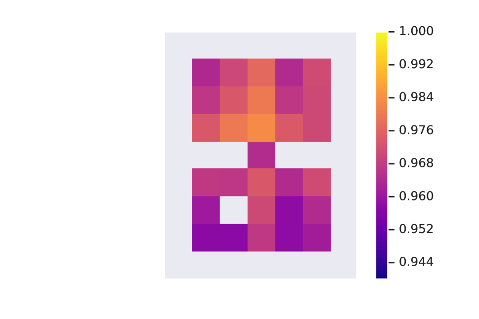
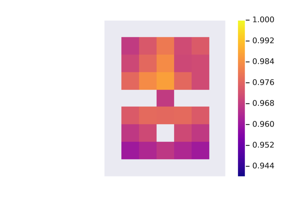
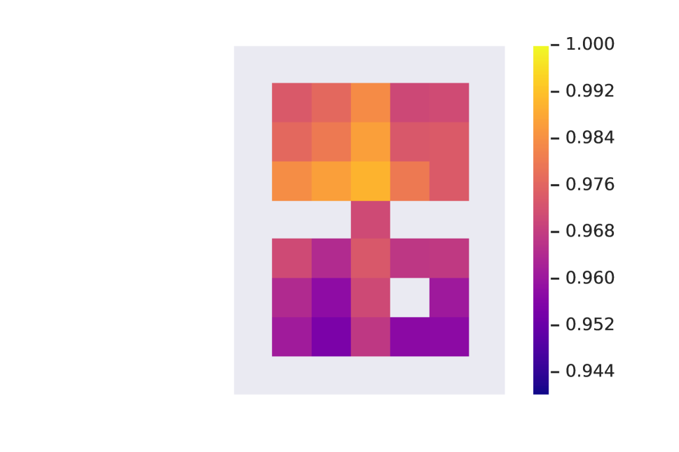
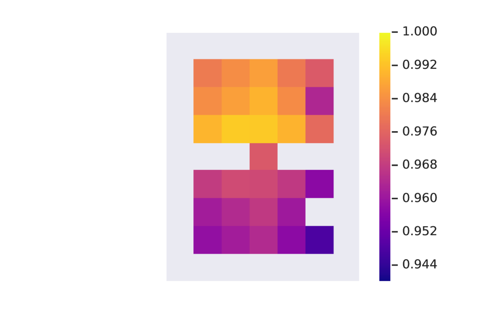
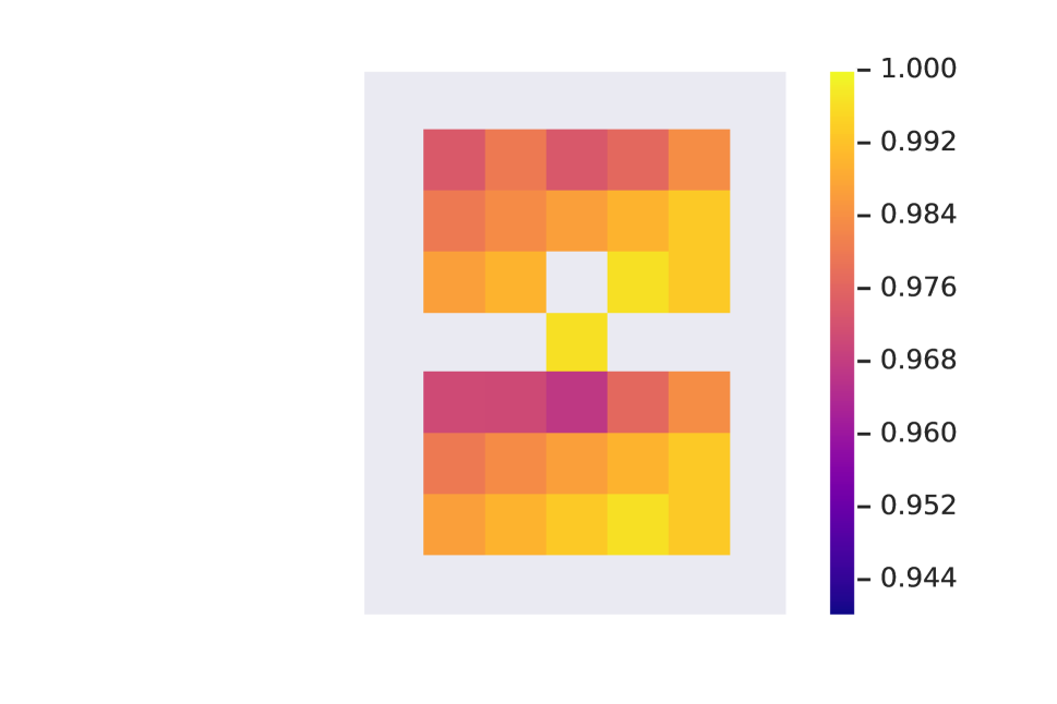
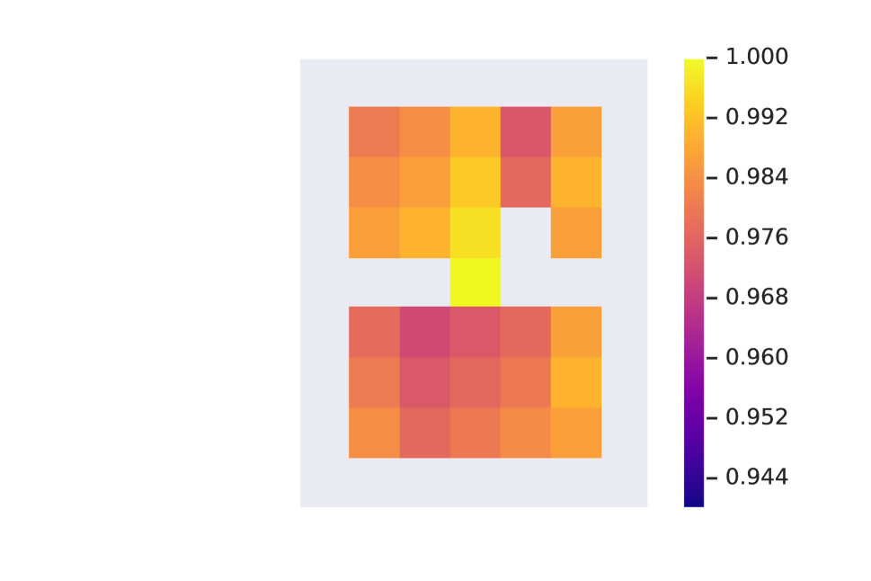
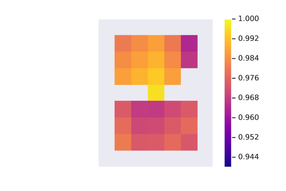
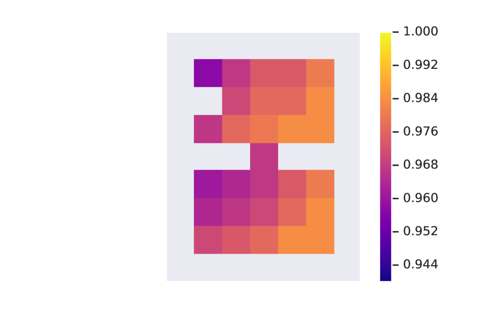
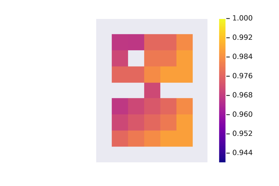
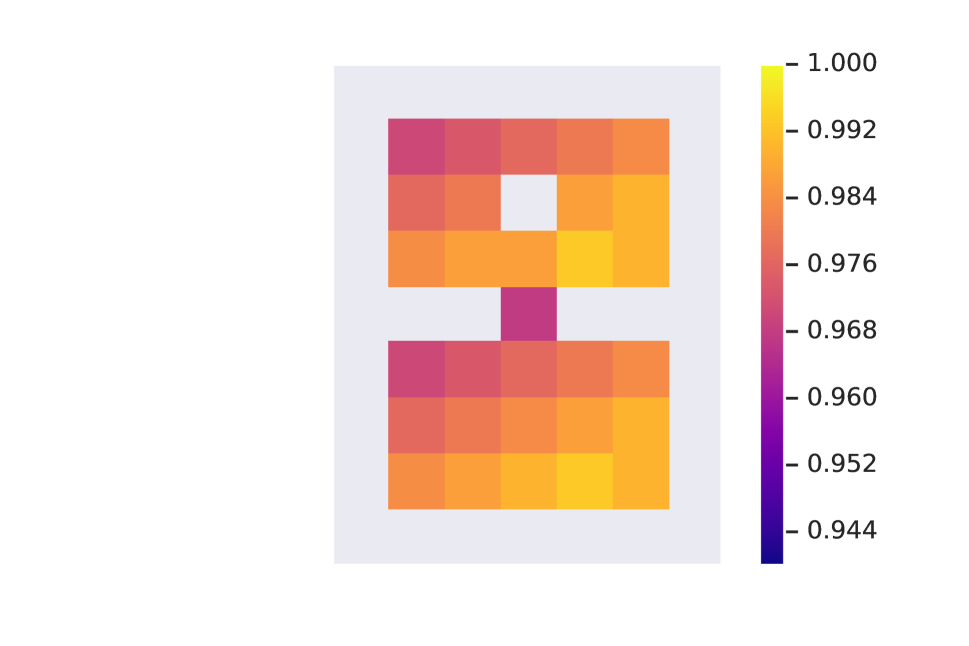
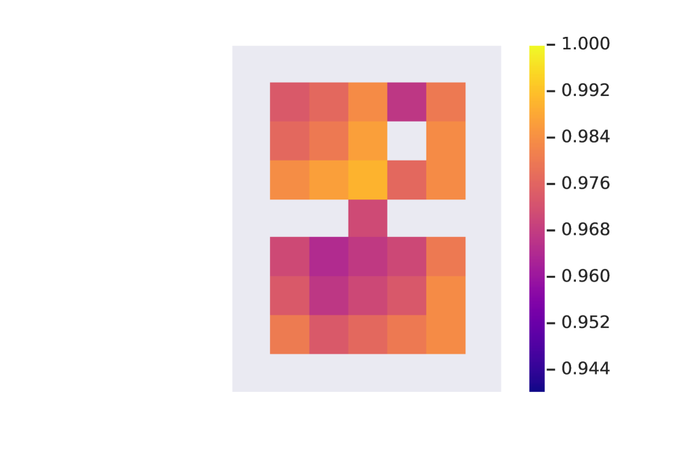
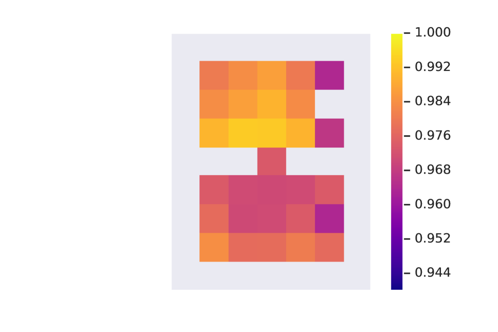
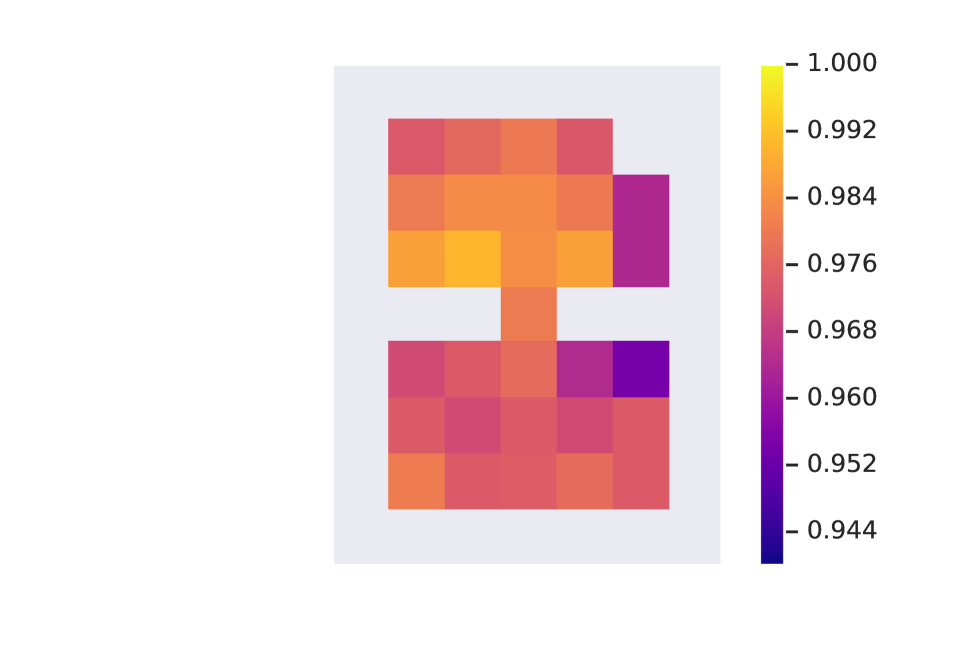
Appendix B Bisimulation distances between all states in the GridWorld
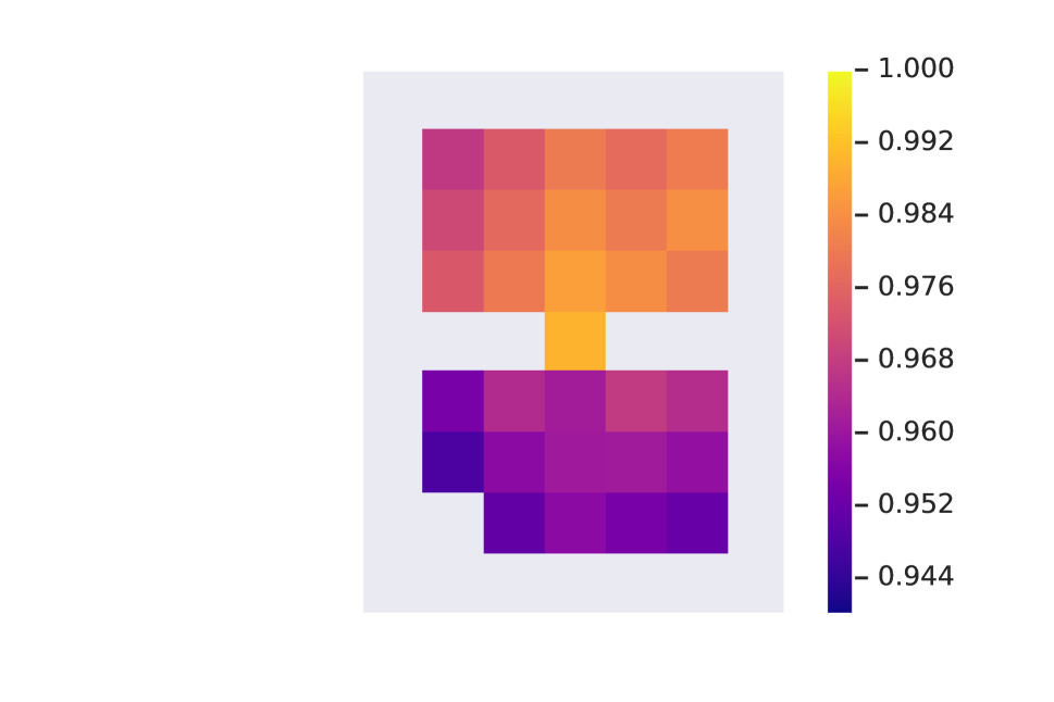
In Figureย 7 we display the bisimulation distances from all states in the GridWorld MDP illustrated in Figureย 4 in the main paper. These were computed using the sampling approach of sectionย 5. Note how $d_{\sim}$ is able to capture similarities that go beyond simple physical proximity. This is most evident when examining the distance from the โ€œhallwayโ€ state to all other states: even though it neighbours the bottom row in the top room, that row is furthest according to $d_{\sim}$.

Refer to caption
Refer to caption
Refer to caption
Refer to caption
Refer to caption
Refer to caption
Refer to caption
Refer to caption
Refer to caption
Refer to caption
Refer to caption
Refer to caption
Refer to caption
Refer to caption
Refer to caption
Refer to caption
Refer to caption
Refer to caption
Refer to caption
Refer to caption
Refer to caption
Refer to caption
Refer to caption
Refer to caption
Refer to caption
Refer to caption
Refer to caption
Refer to caption
Refer to caption
Refer to caption
Refer to caption
Refer to caption
Figure 7: Bisimulation distances from all states.

Appendix C Configuration file for GridWorld

The following configuration file describes the hyperparameters used in subsectionย 7.1.

1GridWorld.gamma = 0.99
2GridWorld.batch_size = 256
3GridWorld.representation_dimension = 729
4GridWorld.num_iterations = 240000
5GridWorld.target_update_period = 500
6GridWorld.starting_learning_rate = 0.01
7GridWorld.use_decayed_learning_rate = False
8GridWorld.learning_rate_decay = 0.9
9GridWorld.epsilon = 1e-8
10GridWorld.staircase = False
11GridWorld.add_noise = True
12GridWorld.bisim_horizon_discount = 0.9
13GridWorld.double_period_halfway = False
14GridWorld.debug = False

Appendix D Aggregating states
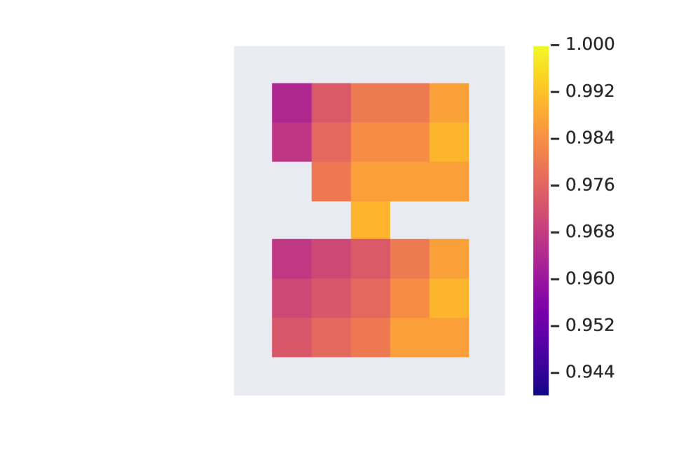
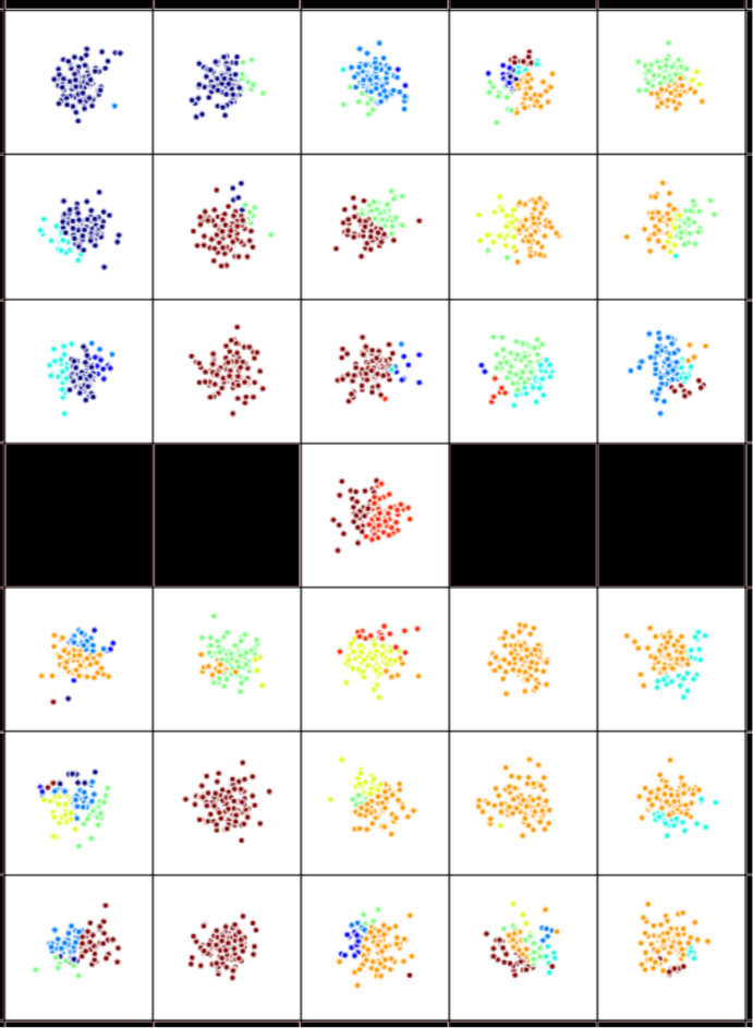
In Figureย 8 we explore aggregating a set of states sampled from the continuous variant of the 31-state MDP. We sampled 100 independent samples for each underlying cell, computed the distances between each pair of sampled states, and then aggregated them by incrementally growing โ€œclustersโ€ of states while ensuring that all states in a cluster are within a certain distance of each other. As can be seen, our learned distance is able to capture many of the symmetries present in the environment: the orange cluster tends to gather near-goal states, the dark-brown and dark-blue clusters seems to gather states further away from goals, while the bright red states properly capture the unique โ€œhallwayโ€ cell. This experiment highlights the potential for successfully approximating bisimulation metrics in continuous state MDPs, which can render continuous environments more manageable.

Refer to caption
Figure 8: Aggregating samples drawn from a continuous MDP using the learned bisimulation metric approximant.

The code for the clustering is displayed below:

1import matplotlib.pyplot as plt
2from matplotlib import cm
3from matplotlib.colors import ListedColormap, LinearSegmentedColormap, BoundaryNorm
4import numpy as np
5
6clusters = []
7threshold = 0.86
8for i in range(len(normalized_distances)):
9 present = False
10 include = False
11 for c in clusters:
12 if np.any(np.isin(i, c)):
13 present = True
14 break
15 present = True
16 for j in c[0]:
17 if normalized_distances[j, i] >= threshold:
18 present = False
19 break
20 if present:
21 np.append(c, i)
22 break
23 if present:
24 continue
25 indices = np.nonzero(normalized_distances[i] < threshold)
26 clusters.append(indices)
27
28labels = np.zeros(len(normalized_distances))
29label = 0
30for c in clusters:
31 for i in c[0]:
32 labels[i] = label
33 label += 1
34cmap = plt.cm.jet
35cmaplist = [cmap(i) for i in range(cmap.N)]
36cmap = cmap.from_list(โ€™Custom cmapโ€™, cmaplist, cmap.N)
37bounds = np.linspace(0,label, label+1)
38norm = BoundaryNorm(bounds, cmap.N)
39fig, ax = plt.subplots(figsize=(16, 16))
40ax.patch.set_facecolor(โ€™whiteโ€™)
41ax.grid(color=โ€™blackโ€™)
42plt.scatter(sampled_distances[โ€™samplesโ€™][:, 1],
43 sampled_distances[โ€™samplesโ€™][:, 0],
44 c=labels, cmap=cmap, norm=norm)
45plt.xlim(0, 7)
46plt.ylim(0, 9)
47plt.colorbar()

Appendix E Distance plots for all games

For each game we display four panels:

  • โ€ข

    Bottom left: Source frame (state s๐‘ s)

  • โ€ข

    Bottom right: Closest frame so far

  • โ€ข

    Top left: Current frame (state $t$)

  • โ€ข

    Top right: Plot of distances from source frame to every other frame (ฯˆฮธฯ€โ€‹([ฯ•โ€‹(s),ฯ•โ€‹(t)])subscriptsuperscript๐œ“๐œ‹๐œƒitalic-ฯ•๐‘ italic-ฯ•๐‘ก\psi^{\pi}_{\theta}([\phi(s),\phi(t)]), in black) and the difference in value function, according to the trained Rainbow network (|V^ฯ€โ€‹(ฯ•โ€‹(s))โˆ’V^ฯ€โ€‹(ฯ•โ€‹(t))|superscript^๐‘‰๐œ‹italic-ฯ•๐‘ superscript^๐‘‰๐œ‹italic-ฯ•๐‘ก|\hat{V}^{\pi}(\phi(s))-\hat{V}^{\pi}(\phi(t))|, in blue)

To pick the hyperparameters, we did a sweep over the following values, performing 3 independent runs for each setting. We picked a setting which gave the best overall performance across all games (final values specified in the $rainbow.gin$ file provided with the source code, except for Pong where we used a learning rate of $0.001$, as specified in the paper):

  • โ€ข

    Learning rates: [0.00005,0.000075,0.0001,0.00025,0.0005,0.00075,0.001]0.000050.0000750.00010.000250.00050.000750.001[0.00005,0.000075,0.0001,0.00025,0.0005,0.00075,0.001]

  • โ€ข

    Batch size: [4,8,16,32,64,128]48163264128[4,8,16,32,64,128]

  • โ€ข

    Target update period: [10,50,100,250,500,1000,2000]105010025050010002000[10,50,100,250,500,1000,2000]

  • โ€ข

    Number of hidden layers: [1,2,3]123[1,2,3]

  • โ€ข

    Number of hidden units per layer: [16,32,64,128]163264128[16,32,64,128]

Refer to caption
Figure 9: Space Invaders: evaluation at frame 500.
Refer to caption
Figure 10: Pong: evaluation at frame 500, peaks are when the agent scores.
Refer to caption
Figure 11: Asterix: evaluation at frame 500. Plateaus are when the agent is not moving.

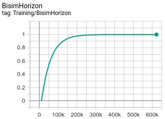
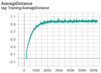
Appendix F Training curves for $d^{\pi}_{\sim}$

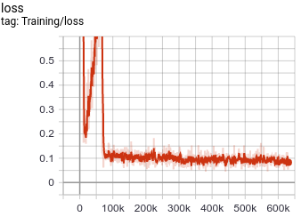
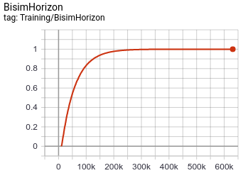
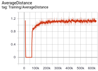
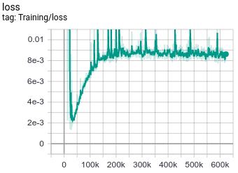
We provide the training curves for the bisimulation metric $d^{\pi}_{\sim}$ learned on the trained reinforcement learning agents.

Refer to caption
Refer to caption
Refer to caption
Figure 12: Training curves for Space Invaders.
Refer to caption
Refer to caption
Refer to caption
Figure 13: Training curves for Asterix.
Refer to caption
Refer to caption
Refer to caption
Figure 14: Training curves for Pong.

Appendix G Lax bisimulation metrics

For completeness, in this section we include the main definitions and theoretical results of lax-bisimulation metrics introduced in (?), modified to match the notation used in this paper.

Definition 5.

A relation $E\subseteq\mathcal{S}\times\mathcal{S}$ is a lax (probabilistic) bisimulation relation if whenever (s,t)โˆˆE๐‘ ๐‘ก๐ธ(s,t)\in E we have that:

  1. 1.

    $\forall a\in\mathcal{A}\exists b\in\mathcal{A}$ such that โ„›โ€‹(s,a)=โ„›โ€‹(t,b)โ„›๐‘ ๐‘Žโ„›๐‘ก๐‘\mathcal{R}(s,a)=\mathcal{R}(t,b)

  2. 2.

    $\forall a\in\mathcal{A}\exists b\in\mathcal{A}.\quad\forall c\in\mathcal{S}_{E}.\mathcal{P}(s,a)(c)=\mathcal{P}(t,b)(c)$,
    where $\mathcal{P}(x,y)(c)=\sum_{z\in c}\mathcal{P}(x,y)(z)$,

The lax bisimulation $\sim_{lax}$ is the union of all lax bisimulation relations.

Definition 6.

Given a $1$-bounded pseudometric $d\in\mathbb{M}$, the metric $\delta(d):\mathcal{S}\times\mathcal{A}\rightarrow[0,1]$ is defined as follows:

ฮดโ€‹(d)โ€‹((s,a),(t,b))=|โ„›โ€‹(s,a)โˆ’โ„›โ€‹(t,b)|+ฮณโ€‹๐’ฒโ€‹(d)โ€‹(๐’ซโ€‹(s,a),๐’ซโ€‹(t,b))๐›ฟ๐‘‘๐‘ ๐‘Ž๐‘ก๐‘โ„›๐‘ ๐‘Žโ„›๐‘ก๐‘๐›พ๐’ฒ๐‘‘๐’ซ๐‘ ๐‘Ž๐’ซ๐‘ก๐‘\delta(d)((s,a),(t,b))=|\mathcal{R}(s,a)-\mathcal{R}(t,b)|+\gamma\mathcal{W}(d)(\mathcal{P}(s,a),\mathcal{P}(t,b))
Definition 7.

Given a finite $1$-bounded metric space $(\mathfrak{M},d)$ let $\mathcal{C}(\mathfrak{M})$ be the set of compact spaces (e.g. closed and bounded in $\mathbb{R}$). The Hausdorff metric $H(d):\mathcal{C}(\mathfrak{M})\times\mathcal{C}(\mathfrak{M})\rightarrow[0,1]$ is defined as:

$$H(d)(X,Y)=\max\left(\sup_{x\in X}\inf_{y\in Y}d(x,y),\sup_{y\in Y}\inf_{x\in X}d(x,y)\right)$$
Definition 8.

Denote Xs={(s,a)|aโˆˆ๐’œ}subscript๐‘‹๐‘ conditional-set๐‘ ๐‘Ž๐‘Ž๐’œX_{s}=\{(s,a)|a\in\mathcal{A}\}. We define the operator $F:\mathbb{M}\rightarrow\mathbb{M}$ as:

Fโ€‹(d)โ€‹(s,t)=Hโ€‹(ฮดโ€‹(d))โ€‹(Xs,Xt)๐น๐‘‘๐‘ ๐‘ก๐ป๐›ฟ๐‘‘subscript๐‘‹๐‘ subscript๐‘‹๐‘กF(d)(s,t)=H(\delta(d))(X_{s},X_{t})
Theorem 5.

$F$ is monotonic and has a least fixed point $d_{lax}$ in which dlโ€‹aโ€‹xโ€‹(s,t)=0subscript๐‘‘๐‘™๐‘Ž๐‘ฅ๐‘ ๐‘ก0d_{lax}(s,t)=0 iff sโˆผlโ€‹aโ€‹xtsubscriptsimilar-to๐‘™๐‘Ž๐‘ฅ๐‘ ๐‘กs\sim_{lax}t.

Theorem 6.

|Vโˆ—โ€‹(s)โˆ’Vโˆ—โ€‹(t)|โ‰คdlโ€‹aโ€‹xโ€‹(s,t)โ‰คdโˆผโ€‹(s,t)superscript๐‘‰๐‘ superscript๐‘‰๐‘กsubscript๐‘‘๐‘™๐‘Ž๐‘ฅ๐‘ ๐‘กsubscript๐‘‘similar-to๐‘ ๐‘ก|V^{*}(s)-V^{*}(t)|\leq d_{lax}(s,t)\leq d_{\sim}(s,t).