Onset of sliding across scales:
How the contact topography impacts frictional strength

Abstract

When two solids start rubbing together, frictional sliding initiates in the wake of slip fronts propagating along their surfaces in contact. This macroscopic rupture dynamics can be successfully mapped on the elastodynamics of a moving shear crack. However, this analogy breaks down during the nucleation process, which develops at the scale of surface asperities where microcontacts form. Recent atomistic simulations revealed how a characteristic junction size selects if the failure of microcontact junctions either arises by brittle fracture or by ductile yielding. This work aims at bridging these two complementary descriptions of the onset of frictional slip existing at different scales. We first present how the microcontacts failure observed in atomistic simulations can be conveniently “coarse-grained” using an equivalent cohesive law. Taking advantage of a scalable parallel implementation of the cohesive element method, we study how the different failure mechanisms of the microcontact asperities interplay with the nucleation and propagation of macroscopic slip fronts along the interface. Notably, large simulations reveal how the failure mechanism prevailing in the rupture of the microcontacts (brittle versus ductile) significantly impacts the nucleation of frictional sliding and, thereby, the interface frictional strength. This work paves the way for a unified description of frictional interfaces connecting the recent advances independently made at the micro- and macroscopic scales.

I Introduction

The rapid onset of sliding along frictional interfaces is often driven by a similar dynamics than the one observed during the rupture of brittle materials. Just like a propagating shear crack, slipping starts and the shear stress drops in the wake of a slip front that is moving along the interface. This analogy particularly suits the observed behaviors of frictional interfaces at a macroscopic scale and explains that the earthquake dynamics has been studied for decades as the propagation of shear cracks along crustal faults [1, 2, 3, 4].

Recent experiments [5] quantitatively demonstrated how Linear Elastic Fracture Mechanics (LEFM) perfectly describes the evolution of strains measured at a short distance from the interface during the dynamic propagation of slip fronts. From this mapping, a unique parameter emerges, the equivalent fracture energy $G_{c}$ of the frictional interface, which was later used to rationalize the observed arrest of slip fronts in light of the fracture energy balance criterion [6, 7]. The same framework was also successfully applied to describe the failure of interfaces after coating the surface with lubricant [8]. Despite a reduction in the force required to initiate sliding, the equivalent fracture energy measured after lubrication was surprisingly higher than for the dry configuration [9]. This apparent paradox in the framework of LEFM is expected to arise during the nucleation phase, which is controlled by the microscopic nature of friction and contact. At the microscale, surfaces are rough and contact only occurs between the surface peaks, resulting in a very heterogeneous distribution of the sliding resistance [10, 11].

A class of laboratory-derived friction models [12, 13, 14] has been successfully used to rationalize some key aspects of the rupture nucleation along frictional interfaces, particularly in the context of earthquakes (critical length scales at the onset of frictional instabilities [13, 15, 16, 17, 18], speed and type of the subsequent ruptures [19, 20, 21, 22, 23]). The so-called rate-and-state formulations are empirically calibrated to reproduce the subtle evolution of friction observed during experiments [10]. A direct connection with the physics of the microcontacts and their impact on the frictional strength remains however unsettled and motivates the recent effort to derive physics-based interpretations of the rate-and-state friction laws [24, 25, 26, 27].

To rationalize the friction coefficient of metal interfaces, Bowden and Tabor [28, 29] suggested that the microcontact junctions represent highly confined regions yielding under a combination of compressive and shear stresses. Later, Byerlee [30] proposed an alternative for brittle materials, by assuming that slipping does not occur through the plastic shearing of junctions but rather by fracturing the microcontacts, which leads to a smaller value of the friction coefficient in agreement with the ones measured for rock interfaces. From atomistic calculations, Aghababaei et al. [31, 32, 33] recently derived a characteristic size of the microcontact junction $d^{*}$ controlling the transition from brittle fracture (of junctions larger than $d^{*}$) to ductile yielding (of junctions smaller than $d^{*}$). As sketched in Fig. 1, these brittle and ductile failure mechanisms co-exist along two rough surfaces rubbing together. From this permanent interplay, Frérot et al. [34] proposed a new interpretation of surface wear during frictional sliding, while Milanese et al. [35] discussed the origin of the self-affinity of surfaces found in natural or manufactured materials. The link between these different microcontact failure mechanisms and the macroscopic frictional strength of the interface remains however overlooked.

In this work, we first present how to approximate the microcontacts failure using a convenient cohesive model. The cohesive approach is then implemented in a high-performance finite element library and used to simulate the onset of sliding across two scales. At the macroscopic level, we study the ability of an interface to withstand a progressively applied shearing, i.e. its frictional strength, while at the microscopic scale, we observe how the failure process develops across the microcontact junctions. This study culminates by discussing how small differences in the interface conditions or the size of asperity junctions, only visible at the scale of the microcontacts, can nevertheless have a significant impact on the nucleation phase and the macroscopic frictional strength.

II Problem description

Figure 1: Geometry of the problem. The inset presents the schematic shear stress $\sigma_{xy}$ profile predicted by LEFM at a distance $r$ from a macroscopic rupture front. A nonlinear region (I) exists at the immediate vicinity of the tip, followed by a linearly elastic region (II), where $\sigma_{xy}$ is dominated by the square root singularity. Further away from the tip (III), non-singular contributions dominate the profile of $\sigma_{xy}$, which converges toward the far-field stress conditions. At the onset of sliding, the microcontacts within the nonlinear region (I) can either break by brittle fracture of their apexes or by plastic yielding [28, 30, 31]. Our work aims at describing how these different failure mechanisms occurring at the scale of asperity contact, i.e. “hidden” within (I), impact the onset of sliding and the frictional strength.

We consider two linearly elastic blocks of height $h/2$ brought into contact along their longitudinal face of length $l$. As presented in Fig. 1, the two blocks are progressively sheared by displacing the top surface at a constant speed ${\dot{\Delta}}_{x}$, while the bottom surface is clamped. In a Cartesian system of coordinates, whose origin stands at the left edge of the contacting plane, the boundary conditions of this elastodynamic problem correspond to

$$\left\{\begin{aligned} &\bm{u}(x,-h/2,t)=0\\ &{\dot{u}}_{x}(x,h/2,t)={\dot{\Delta}}_{x}\\ &u_{y}(0,y,t)=u_{y}(l,y,t)=0\end{aligned}\right.$$ (1)

and lead to a state of simple shear, for which the shear components of the Cauchy stress tensor are $\sigma_{xy}=\sigma_{yx}=\tau$. In Eq. (1), $\bm{u}=\{u_{x},u_{y}\}$ corresponds to the displacements vector and $\dot{\square}$ denotes a time derivative. The elastodynamic solution of this system in the absence of interfacial slip is presented in Fig. A1 of the Appendix. As illustrated in Fig. 1, sliding nucleates at small scales from the rupture of the microcontacts which potentially stems from several non-linear phenomena (cleavage, plasticity, interlocking). As discussed by Aghababaei et al. [31], atomistic models are particularly suited to simulate these phenomena in comparison to continuum approaches, but are conversely disconnected from the macroscopic dynamics. Therefore, we rely on a 2D plane strain continuum description of the two solids, while the complex interface phenomena and associated dissipative processes are assumed to be constrained at the contact plane and entirely described by a “coarse-grained” cohesive law deriving from a thermodynamic potential $\Phi$. The shape of $\Phi$ and its associated exponential cohesive law correspond to a generic failure response of the microcontact asperities observed during a large set of atomistic simulations [31, 32, 36, 33, 35, 37, 38]. As sketched in Fig. 1, sliding is assumed to initiate at the edge of a critical nucleus (e.g. the largest non-contacting region or the result of underlying stochastic processes [21, 39]) existing at the very left of our model interface with a size $w_{0}$. Moreover, the rough contact topography sketched in Fig. 1 is idealized as a regular pattern of contacting and non-contacting junctions of microscopic size $w\ll w_{0}$.

Additional details about theoretical derivations, the numerical method and the material properties used in this manuscript are provided in Appendix, which namely defines the values of the Young’s modulus $E$, the Poisson’s ratio $\nu$ and a reference interface fracture energy $G_{c}^{\rm ref}$.

III Characteristic length scales of the brittle-to-ductile failure transition

Figure 2: The ratio of the process zone size to the length of the junction mediates the work required to initiate sliding. (a) Normalized external work required to initiate sliding along a single uniform junction as function of the ratio between the process zone size $l_{pz}$ and the resisting junction size $(l-w_{0})$ for different types of interface properties and geometries. (b) and (c) present the evolution of energies during the onset of sliding, which occurs respectively at $t=92t^{*}$ and $t=35t^{*}$. The two events share the same elastic properties and $G_{c}=4G_{c}^{\rm ref}$, but their respective interface cohesive laws lead to $l_{pz}/(l-w_{0})=3.5\cdot 10^{-2}$ and $l_{pz}/(l-w_{0})=3.5$. The dashed lines in (b) and (c) present the build-up of elastic strain energy in the absence of interfacial slip discussed in the Appendix.

Next, we study the onset of slip along a uniform and homogeneous interface (i.e. a unique junction) of fracture energy $G_{c}$ and size $(l-w_{0})$. Figure 2b presents the evolution of energies observed during a typical failure event, i.e, the applied external work $W_{\textmd{ext}}$, the elastic strain energy $E_{\textmd{el}}$, the energy dissipated by fracture $E_{\textmd{frac}}$, and the kinetic energy $E_{\textmd{kin}}$. During an initial phase, the elastic strain energy builds up in the system following the dynamics predicted in the absence of interfacial slip (Fig. A1) and depicted by the black dashed line. After an initial loading phase, sliding nucleates at $x=w_{0}$, a propagating slip front breaks the interface cohesion and releases $E^{*}_{\textmd{frac}}=G_{c}(l-w_{0})$. The asterisk marks in Figs. 2b-c simply distinguish the final value of energy obtained after the complete interface failure from its transient value, i.e. $E_{i}^{*}=E_{i}(t\gg t^{*})$. After the complete failure, an eventual excess of mechanical energy ($W^{*}_{\textmd{ext}}-E^{*}_{\textmd{frac}}$) remains in the system and takes the form of elastic vibrations in absence of any other dissipative process.

Figure 2c describes the evolution of energies observed during another failure event, during which sliding initiates for a significantly lower applied external work, exactly balancing the energy dissipated in fracture ($W^{*}_{\textmd{ext}}=E^{*}_{\textmd{frac}}$). Perhaps surprisingly to some readers, these quantitatively different sliding events arise within two systems having identical elastic properties ($E$, $\nu$) and interface fracture energy $G_{c}$. These different dynamics emerge solely from the size of the fracture process zone at the tip of the crack which can be estimated as [40, 41]:

$$l_{pz}\cong e\frac{\delta_{c}}{\tau_{c}}\frac{E}{(1-\nu^{2})}=\frac{G_{c}}{\tau_{c}^{2}}\frac{2\mu}{1-\nu}.$$ (2)

$\tau_{c}$ and $\delta_{c}$ are respectively the maximum shear strength and critical slip displacement entering the cohesive formulation (see Eqs. (A14) and (A15)). When the size of the process zone $l_{pz}$ is comparable to the junction size $(l-w_{0})$, the sliding motion develops along a damage band stretching over the entire length of the interface with an energy balance similar to the one observed in Fig. 2c. Conversely, if $l_{pz}\ll(l-w_{0})$, sliding initiates in the form of a slip front propagating from $x=w_{0}$ and leading to a more violent rupture as described in Fig. 2b. The two different stress profiles existing prior to the rupture events presented in Fig. 2b and c can be visualized in Fig. A2 of the Appendix. In the limit of an infinitesimally small process zone, the rupture corresponds to a singular shear (mode II) crack, whose propagation initiates according to LEFM energy balance. In this context, the applied external work should not solely balances $E^{*}_{\rm frac}$ but also load the system above the strain energy required to initiate the rupture. The latter is derived in the Appendix and can be estimated as ($\chi\approx 1.12$):

$$E^{\textmd{lefm}}_{\textmd{el}}=\frac{G_{c}}{\chi^{2}}\frac{hl}{\pi w_{0}(1-\nu)}.$$ (3)

For different interface properties and dimensions, Fig. 2a presents how the process zone size (Eq. (2)) together with the rupture energy balance can rationalize the observed transition from the dynamics of sharp crack-like events (for $l_{pz}\ll(l-w_{0})$) to gradual ductile failures (for $l_{pz}\geqslant(l-w_{0})$).

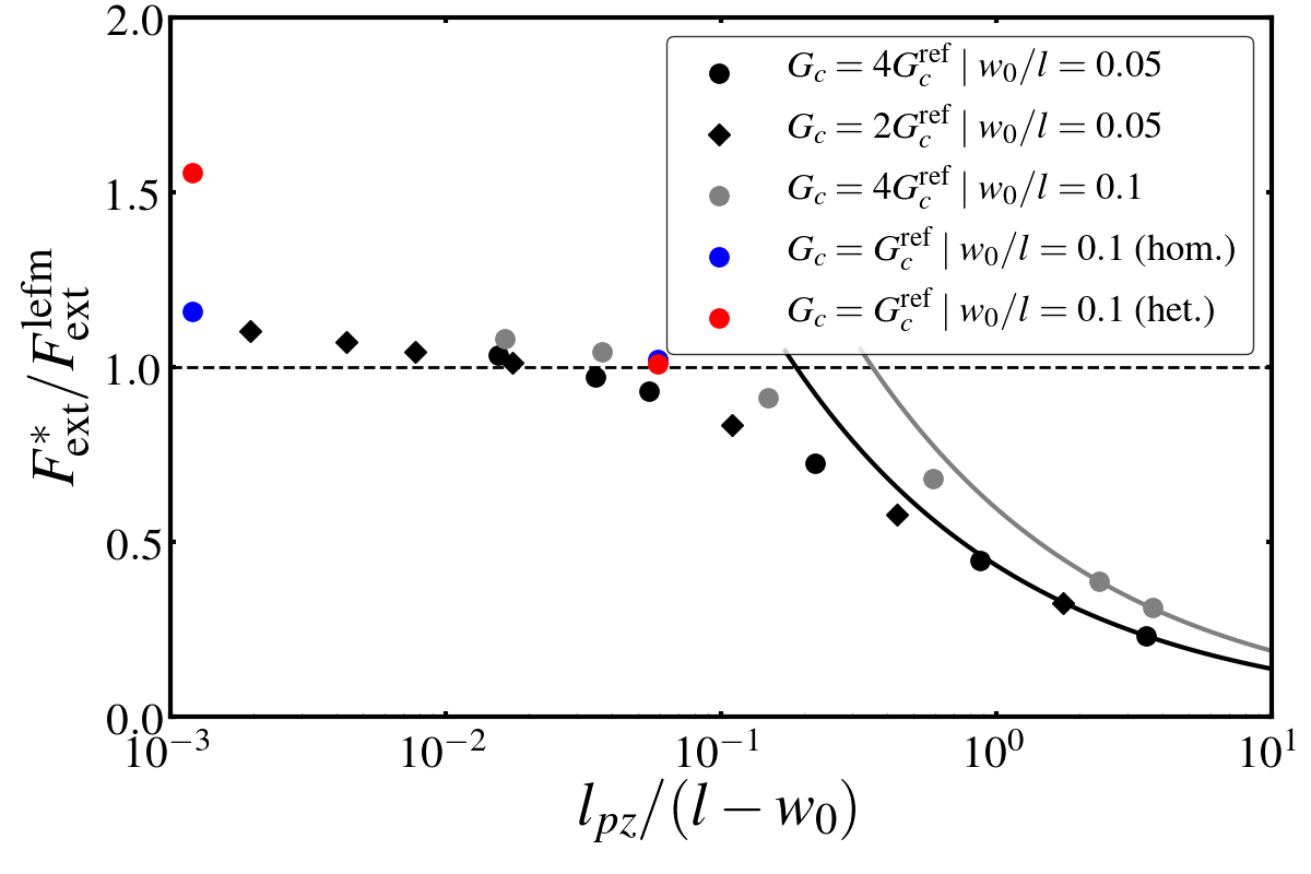
Figure A3: External force required to trigger sliding as function of the process zone size for the simulations reported in the Figs. 2a and 3a of the manuscript. In the large process zone limit, the data follows $F^{\rm str}_{\textmd{ext}}$, whose evolution predicted by Eq. (4) is depicted by the black and grey solid lines for the two studied geometries, respectively $w_{0}/l=0.05$ and $w_{0}/l=0.1$. With shorter process zone sizes, the external force saturates at $F^{\rm lefm}_{\textmd{ext}}$, the value predicted from brittle fracture. The blue and red dots present the values observed for respectively the homogeneous and heterogeneous large-scale simulations. Please refer to the presentation in the main text for more information about the different setups.

In some applications, the system is preferably described in terms of the macroscopic force $F^{*}_{\textmd{ext}}$ required to trigger sliding, i.e. to reach the interface frictional strength. As presented in Fig. A3, the brittle-to-ductile transition can be similarly characterized from the evolution of the force required to initiate sliding between $F^{\rm lefm}_{\textmd{ext}}$ and $F^{\rm str}_{\textmd{ext}}$. Using Eqs (2) and (A10), $F^{\rm str}_{\textmd{ext}}$ can be rewritten as

$$F^{\rm str}_{\textmd{ext}}=F^{\rm lefm}_{\textmd{ext}}\Big{(}\frac{l_{pz}}{l-w_{0}}\Big{)}^{-\frac{1}{2}}\sqrt{\chi^{2}\pi\frac{w_{0}}{l}\Big{(}1-\frac{w_{0}}{l}\Big{)}}.$$ (4)

This expression is depicted by the black and gray solid lines in Fig. A3 and predicts well the evolution of the frictional force observed when the process zone is large. With very small process zones, the frictional force saturates at the value predicted by brittle fracture theory in Eq. (A10).

The evolution between these two failure mechanisms reported in Figs. 2a and A3 is analogous to the transition discussed in the tensile failure of concrete structures [42] from the plastic failure of small specimens to the brittle failure of larger structures. Two important differences arise during the shear failure of frictional interfaces. Brittle and ductile mechanisms co-exist during the failure of rough surfaces and the characteristic length scale is not purely a bulk property but also depends on interface conditions (for example lubrication). Indeed, an equivalent brittle-to-ductile transition exists in the failure of the microcontact asperities observed in the atomistic simulations. Aghababaei et al. [31] revealed how a characteristic junction size

$$d^{*}=\lambda\frac{G_{c}}{\tau_{c}^{2}}\mu$$ (5)

mediates this transition from the brittle rupture of the apexes of junctions larger than $d^{*}$ to the ductile yielding of junctions smaller than $d^{*}$. In Eq. (5), $\lambda$ is a dimensionless factor accounting for the geometry (typically in the range of unity) and, therefore, $l_{pz}$ (Eq. (2)) corresponds to the same characteristic length scale than $d^{*}$ (Eq. (5)). Remarkably, there is a direct analogy between the brittle-to-ductile failure transition (controlled by $d^{*}$) observed during the failure of microcontact asperities [31] and the failure of the “coarse-grained” junctions (controlled by $l_{pz}$) presented in Fig. 2a using the cohesive approach. The latter represents therefore a powerful tool to unravel the impact of the microcontacts failure on the macroscopic frictional strength of multi-asperity interfaces.

Next, we select two types of interface properties with the same fracture energy $G_{c}=G_{c}^{\rm ref}$ and with process zone sizes that are much smaller than the size of the domain. We later refer to these two systems as interface A ($l_{pz,A}/l=9\cdot 10^{-4}$) and interface B ($l_{pz,B}/l=4.5\cdot 10^{-2}$). For the single-junction interfaces considered in this section, the interfaces A and B rupture with a crack-like dynamics (as $l_{pz}\ll l-w_{0}$) at similar magnitudes of external work (see the blue circles in Fig 2a, which are recalled in Fig 3a). In the next section, the frictional strength of multi-asperity interfaces is studied in light of the characteristic junction size $d^{*}$. The size of the microcontact junctions $w$ is chosen in order to discuss the cases where $w$ is respectively larger/smaller than the characteristic junction size of the interfaces A/B ($d^{*}_{A}<w<d^{*}_{B}$). The characteristic junction sizes are computed using $\lambda\cong 3$ in Eq. (5), such that $d^{*}\equiv l_{pz}$. This value of $\lambda$ corresponds to the one estimated for three-dimensional spherical asperities in [31].

IV Rough contact topography and frictional strength

Figure 3: Evolution of the frictional strength in the presence of microcontact junctions for two representative interfaces differentiated by their respective characteristic junction size ($d^{*}_{A}<w<d^{*}_{B}$). (a) The grey circles recall the data discussed previously in Fig. 2a. The blue circles corresponds to homogeneous (single junction) interfaces. The red circles are associated to multi-asperity interfaces with a heterogeneous microstructure but the same average fracture energy $G_{c}^{\rm ref}$. (b)-(c) Zooms at the vicinity of the critical nucleus $(x=w_{0})$ revealing the origin of the frictional strength difference between interface A and B in the presence of microcontacts. Colors depict the shear stress profile existing before the onset of sliding while an artificial vertical displacement $\Big{(}u_{y}(x,y)=u_{x}(x,y)\Big{)}$ is applied to help visualizing the slip profile along the interface ($200$ times magnification). The evolution of junctions strength is depicted with a gradation from black ($\tau^{\mathrm{str}}=\tau_{c}$) to white ($\tau^{\mathrm{str}}=0$). The sketches located in the top right of each plot associate the failure of the coarse-grained multicontacts interfaces A and B to the corresponding failure mechanism of surface asperities discussed in Fig. 1.

As sketched in Fig. 1, two solids come into contact along a reduced portion of the interface, between the peaks of the microscopically rough surfaces. To model the effect of this heterogeneous topography, we now introduce an idealized array of microscopic gaps and junctions of size $w=0.05w_{0}=0.005l$. In order to keep the total energy dissipated into fracture unchanged ($E^{*}_{\textmd{frac}}=G_{c}^{\rm ref}(l-w_{0})$), the fracture energy of the microscopic junctions is set to $2G_{c}^{\rm ref}$. The interfaces A and B have significantly different frictional strength in presence of the heterogeneous microstructure as shown by the red circles in Fig. 3a for the external work and in Fig. A3 for the external force. This major difference is caused by the introduction of a new length scale $w$ in the systems, which exactly stands between the characteristic length scales $d^{*}_{A}$ and $d^{*}_{B}$.

As presented in Fig. 3c, along interface B ($d^{*}_{B}>w$), several microcontact junctions start damaging and slipping during the initial loading phase. The stress concentration at the edge of the critical nucleus spans several microcontact junctions and gaps. Their individual properties are thereby homogenized within this large process zone and result in a quasi-homogeneous frictional response driven by the strength-dominated ductile failure. Conversely, for interface A ($d^{*}_{A}<w$), the shear stress sharply concentrates at the very edge of the microcontact junctions (cf. Fig. 3b) whose local toughness directly controls the onset of failure.

For interface B, the effective fracture energy corresponds to the average value which explains that the heterogeneous and homogenized interfaces break at the same magnitudes of $W^{*}_{\textmd{ext}}$ and $F^{*}_{\textmd{ext}}$. For interface A, the toughness of the microcontact junctions ($G_{c}=2G^{\rm ref}_{c}$) directly controls the failure. From Eqs. (A9) and (A10), the external work and the external force are hence expected to increase by respectively a factor $2$ and $\sqrt{2}$, in good agreement with the simulated values (reported in Figs. 3 and A3). Such toughening mechanism can therefore become stronger if a larger contrast exists between the toughness of individual microcontacts and the average macroscopic toughness of the interface.

V Subsequent rupture dynamics

The main objective of the manuscript is to study the impact of the microscopic roughness at nucleation. It is nevertheless insightful to briefly comment the subsequent rupture dynamics observed along the heterogeneous interfaces A and B. As shown in the previous sections, the details of the microstructure plays an important role during the nucleation phase as the macroscopic frictional strength cannot be systematically predicted from the average interface properties. However, the subsequent rupture dynamics are macroscopically similar and comply with LEFM predictions for homogenized interface properties. In Fig. 4, the stress profiles are measured at a macroscopic distance ($h/25\gg w$) from the contacting plane as it is the case during experiments [5, 7, 8]. In both situations, the stress profiles present the K-dominance predicted by LEFM for dynamic shear cracks with an associated dynamic energy release rate balancing the average fracture energy $G_{c}^{\rm ref}$. The details of the linear elastic stress solutions used in Fig. 4 are described in Appendix.

Figure 4: At a macroscopic distance from the interface the evolutions of the stress fields observed during the dynamic failure of the heterogeneous interfaces A (top) and B (bottom) comply with LEFM predictions for an interface fracture energy corresponding to the average value $G_{c}^{\rm ref}$. On the left panels, shear stress at the vicinity of the propagating slip front is mapped using the same color scale. To mimic the experimental measurements, the white lines highlight the position along which the components of the Cauchy stress tensor are presented on the right panels in red. The stress fields predicted by LEFM at the vicinity of a shear crack are plotted in blue for a fracture energy equal to $G_{c}^{\rm ref}$. Note that the mismatch visible in the simulation profiles of $\sigma_{xy}$ is caused by the shear wave traveling ahead of an accelerating shear crack which is not included in LEFM solutions of Eq. (A18) [43, 44].

Few differences need to be commented; As $d^{*}$ significantly impacts the nucleation, dynamic rupture initiates under higher shear stress along interface A than B and consequently propagates at faster velocities. Both explain the different stress amplitudes between the two interfaces in Fig. 4. The high frequency radiations visible in the stress profile of interface A are another difference arising from the interplay of dynamic ruptures with heterogeneities larger than the process zone [45], and therefore mainly for interface A. Nevertheless, their wavelength and amplitude are expected to decay for microcontacts smaller than the two orders of magnitude considered in our simulations and become out of the resolution of macroscopic experiments. Finally, additional differences could exist for 3-dimensional systems. Indeed, the in-plane distortions of the slip front caused by tough asperities larger than $d^{*}$ (as in configuration A) could cause intense stress concentrations strongly impacting the overall rupture dynamics (as reported in the context of dynamic fracture [46, 47]).

VI Discussion and concluding remarks

Between two realistic rough surfaces in contact, a dense spectrum of junction sizes forms the real contact area, which often barely exceeds few percents of the apparent area of the contact plane [10]. The contacting asperities form clusters whose sizes typically follow a power-law distribution [48]. Moreover, the strength of each asperity could vary following Gaussian or Weibull distribution. In this context, our results predict the length under which the details of the microstructure can be homogenized along the tip of a nucleating slip patch. Interestingly, this length is equivalent to the characteristic junction size $d^{*}$ used to study the formation of wear particles [31, 34]. Indeed, the strength of the junctions smaller than $d^{*}$ can be averaged (cf. responses of interface B in Fig. 3a), whereas the toughness of the microcontact junctions larger than $d^{*}$ are individually impacting the macroscopic frictional behavior of the interface (cf. responses of interface A in Fig. 3a). The combination of the criterion described in this paper with models simulating the contact of two rough surfaces [11, 49] open new prospects to investigate the frictional strength of contact interfaces. Such models could notably account for three-dimensional effects (e.g. shear-induced anisotropy [50], shielding of neighboring rupture fronts [36] or its pinning by tough asperities [51]).

Any modification of the characteristic junction size $d^{*}$ (lubrication, coating) or the microcontact topography (sanding) will thereby impact the macroscopic frictional strength (even if such modifications are only visible at a microscale and do not change the average interface properties). The brittle-to-ductile transition discussed in this work brings then an interesting avenue to rationalize the “slippery but tough” behavior of lubricated interfaces discussed in the introduction. As reported by Bayart et al. [9], the lubrication significantly increases the critical slip distance $\delta_{c}$ and the interface fracture energy $G_{c}$. Moreover, a reduction of the interface adhesion also leads to an increase of the characteristic junction size $d^{*}$ [37, 38]. Dry contact can hence be viewed as a strong but fragile interface, where slip initiates by a sharp concentration of the shear stress and damage zone at the edge of the microcontacts, followed by the abrupt brittle failure of individual microcontacts. After lubrication, the damage zone distributed over multiple microcontacts leads to the strength-dominated ductile failure of several junctions, resulting macroscopically into a more slippery yet tougher interface.

Whereas the microcontacts topography together with $d^{*}$ play a significant role at nucleation, the macroscopic rupture dynamics appears to be much less impacted by the microscopic details and comply with the theoretical predictions for average homogenized properties. This observation is in good agreement with a recent set of frictional experiments revealing how the fracture energy inverted from interfacial displacements shows significant variations around the average and uniform value inverted from strain measurements in the bulk [52].

More broadly, this work also find implications in our understanding of the failure of heterogeneous media, particularly in the context of multi-scale and hierarchical materials, for which the microstructure organization can be tuned to enhance the overall material properties [53, 54].

VII APPENDIX

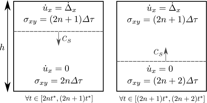
Figure A1: Elastodynamic solution in the absence of interfacial slip. The dynamic fields are mediated by the vertical propagation of a shear wave front characterized by $\varDelta\tau=\mu/c_{s}\;{\dot{\Delta}}_{x}$. $t^{*}=h/c_{s}$ is the time needed by the front to travel between the top and bottom surfaces and $n\in\mathbb{N}$ is the total number of reflections observed at the top boundary.

Appendix A End-member elastic solutions

The numerical results presented in the manuscript are supported by theoretical solutions derived hereafter in the framework of linear elasticity which rests upon the following momentum balance equation:

$$\nabla\cdot\bm{\sigma}(x,y,t)=\rho\ddot{\bm{u}}(x,y,t).$$ (A1)

In the equation above, $\nabla$ is the divergence operator and we recall that $\bm{\sigma}$ is the Cauchy stress tensor, $\bm{u}$ the displacements vector and $\ddot{\square}$ denotes a double time derivative. At time $t=0$, the two continua presented in Fig. 1 are initially at rest and start being progressively loaded by a shear wave whose amplitude corresponds to $\varDelta\tau=\mu/c_{s}\;{\dot{\Delta}}_{x}$. $\mu$ is the elastic shear modulus and $c_{s}$ the shear wave speed such that $t^{*}=h/c_{s}$ is the wave travel time between the top and bottom surfaces. Figure A1 presents the elastodynamic solution of this system under the boundary conditions listed in Eq. (1). In this state of simple shear, the only non-zero components of $\bm{\sigma}$ are the shear stress $\sigma_{xy}=\sigma_{yx}=\mu\partial u_{x}/\partial y$ such that the elastic strain energy reduces to

$$E_{\rm el}=\frac{1}{2\mu}\int_{-\frac{h}{2}}^{\frac{h}{2}}\int_{0}^{l}(\sigma_{xy})^{2}dxdy.$$ (A2)

Integrating the stress of the solution presented in Fig. A1 according to Eq. (A2) leads to the quadratic build-up of strain energy depicted by the black dash lines in Figs. 2b and 2c.

After an initial loading phase, the build-up of strain energy is limited by the nucleation of slip and the progressive failure of the interface. As the system is initially at rest, the energy conservation implies that

$$E_{\rm pot}+E_{\rm kin}+E_{\rm frac}=0.$$ (A3)

$E_{\rm pot}=E_{\rm el}-W_{\rm ext}$ is the potential energy, such that Eq. (A3) can be rewritten after the complete interface failure as

$$E_{\rm el}+E_{\rm kin}=W^{*}_{\rm ext}-E^{*}_{\rm frac}.$$ (A4)

As discussed in the manuscript, the right-hand-side terms of Eq. (A4) reaches constant values, respectively $W^{*}_{\rm ext}$ and $E^{*}_{\rm frac}$, while the left-hand-side terms represent an eventual excess of mechanical energy remaining in the system after the rupture.

As function of the size of the region where sliding nucleates (i.e. the process zone size $l_{pz}$), two end-member situations exist. In the limit of an infinitesimally small process zone, this excess of mechanical energy can be related to the energy barrier governing the nucleation of a singular shear (mode II) crack. From Linear Elastic Fracture Mechanics (LEFM) [55, 56, 57], the rupture propagation starts according to the following thermodynamic criterion:

$$K_{II}>K_{c}.$$ (A5)

In the equation above, $K_{c}$ is the interface fracture toughness, which can be computed from the fracture energy as

$$K_{c}=\sqrt{G_{c}\frac{E}{(1-\nu^{2})}}.$$ (A6)

$K_{II}$ is the stress intensity factor, which depends on the far-field shear stress $\sigma^{\infty}_{xy}$, the initial crack size ($w_{0}$ in our setup) and a dimensionless factor $\chi$ accounting for the geometry:

$$K_{II}=\chi\sigma^{\infty}_{xy}\sqrt{\pi w_{0}}.$$ (A7)

In this manuscript, $\chi$ is approximated as $1.12$ for the edge crack configuration of interest [57]. The rupture is then expected to initiate when

$$\sigma_{xy}\geq\sigma^{\infty}_{xy}=\frac{1}{\chi}\sqrt{\frac{G_{c}}{\pi w_{0}}\frac{E}{(1-\nu^{2})}}.$$ (A8)

By assuming homogeneous shear stress within the two solids, the elastic strain energy required to initiate the rupture can be approximated by

$$E^{\rm lefm}_{\rm el}=\frac{1}{2\mu}\int_{-\frac{h}{2}}^{\frac{h}{2}}\int_{0}^{l}(\sigma^{\infty}_{xy})^{2}dxdy=\frac{G_{c}}{\chi^{2}}\frac{hl}{\pi w_{0}(1-\nu)},$$ (A9)

which represents a strain energy barrier governing the onset of rupture growth. In the limit of a process zone larger than the length of the interface, the failure progressively occurs everywhere along the contact plane once the shear stress reaches the interface strength $\sigma_{xy}=\tau_{c}$ such that no energy barrier exists and $W^{*}_{\rm ext}=E^{*}_{\rm frac}$.

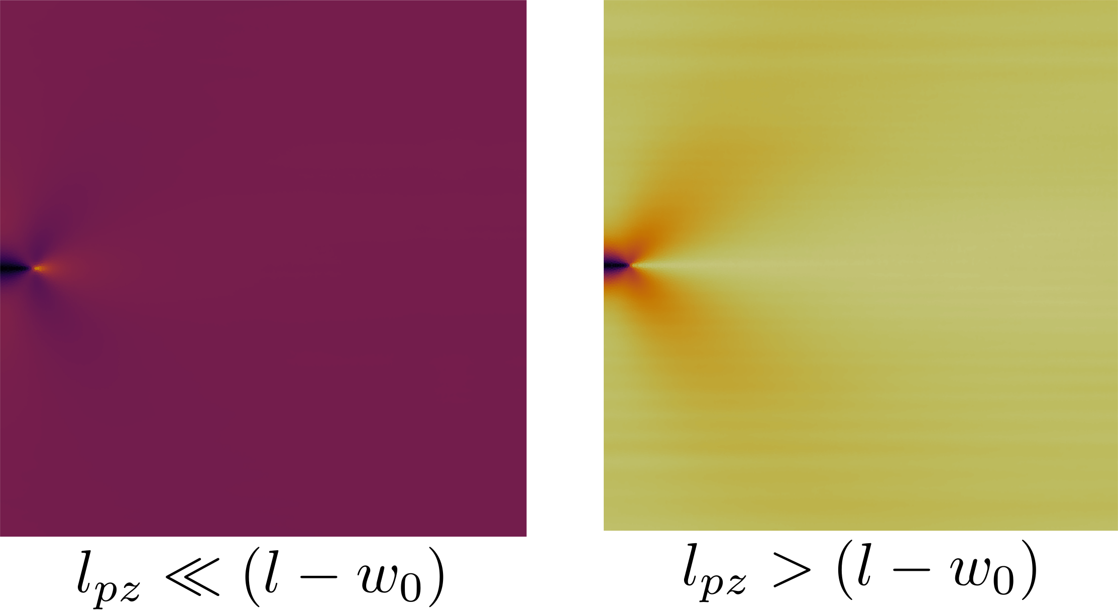
Figure A2: Shear stress profiles before the onset of sliding for the two different failure mechanisms selected by the size of the process zone. In the left plot ($l_{pz}\ll(l-w_{0})$), the stress concentrates at the very edge of the junction and the subsequent rupture corresponds to the sharp crack-like event studied in Fig. 2b. In the right plot ($l_{pz}>(l-w_{0})$), the stress is uniform over the junction and leads to the ductile failure presented in Fig. 2c.

Figure A2 presents the shear stress profiles existing for these two end-member situations prior to the rupture. In the manuscript, this transition is studied in terms of the energy balance but the same approach could be used to predict the macroscopic force $F^{*}_{\textmd{ext}}$ required to trigger sliding, i.e. to reach the interface frictional strength. Invoking that the dynamic effects are negligible before the onset of sliding, two end-member solutions can be similarly derived for $F^{*}_{\textmd{ext}}$. In the limit of an infinitesimal process zone ($l_{pz}\ll(l-w_{0})$), the force is controlled by the far-field shear stress predicted by LEFM and corresponds to

$$F^{\rm lefm}_{\textmd{ext}}=\sigma^{\infty}_{xy}\cdot l=\frac{l}{\chi}\sqrt{\frac{G_{c}}{\pi w_{0}}\frac{E}{(1-\nu^{2})}}.$$ (A10)

Conversely, if $l_{pz}>(l-w_{0})$ the applied force should balance the peak strength along the entire contact junction such that $F^{*}_{\textmd{ext}}$ approaches

$$F^{\rm str}_{\textmd{ext}}=\tau_{c}\cdot(l-w_{0}).$$ (A11)

Appendix B Numerical method

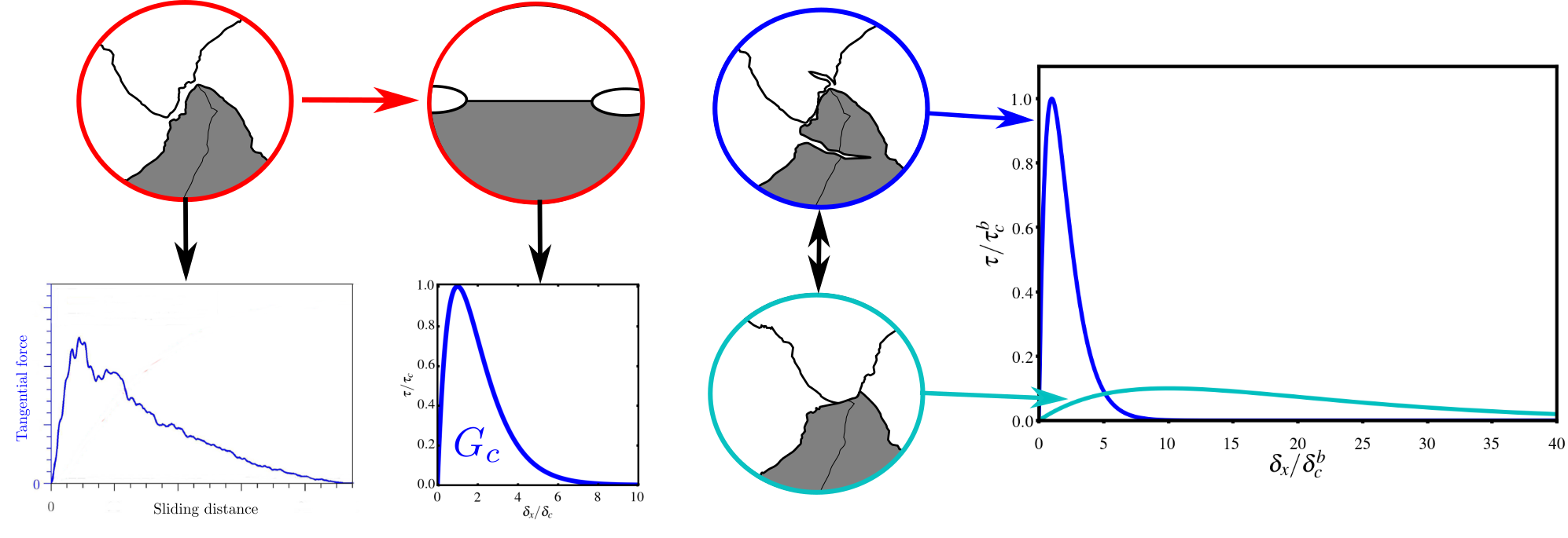
Figure A4: From left to right: Typical force versus slip profile observed during the shearing of two interacting asperities in molecular dynamics simulations (see [32] for a detailed presentation of the method and setup). Such behavior can be conveniently described by the exponential cohesive law given in Eq. (A14) and derived from a Rose-Ferrante-Smith [58] type of universal binding potential. The exponential cohesive law allows for saving the cost of describing the fine details of asperity contact and, in return, the coarse-grained junctions can embed the microcontacts failure behavior into the macroscopic response of frictional systems. More notably, these coarse-grained junctions also reproduce the essential observations of the molecular dynamics simulations: the brittle-to-ductile transition in the failure of microcontact junctions controlled by an identical characteristic length scale (see the discussion in Section Characteristic length scales of the brittle-to-ductile failure transition of the manuscript). Examples of a very brittle cohesive law in dark blue ($\tau^{b}_{c}$; $\delta^{b}_{c}$) and a more ductile one in cyan ($\tau^{d}_{c}=0.1\tau^{b}_{c}$; $\delta^{d}_{c}=10\delta^{b}_{c}$) having the same fracture energy.

The elastodynamic equation (Eq. (A1)) is solved with a finite element approach using a lumped mass matrix coupled to an explicit time integration scheme based on a Newmark-$\beta$ method [59]. The stable time step is defined as function of the dilatational wave speed $c_{d}$ and the spatial discretization $\Delta s$ as

$$\Delta t=0.7\frac{\Delta s}{c_{d}},$$ (A12)

with $\Delta s$ being typically set to $\frac{l}{1000}$ in this work. For the large simulations of interfaces with a heterogeneous microstructure, the discretization is brought to $\frac{l}{5000}$ leading to about 70M degrees of freedom. The virtual work contribution of the frictional plane is written as

$$\hat{W}(t)=\int_{0}^{l}\tau(x,t)\hat{\delta}_{x}(x,t)dx,$$ (A13)

with $\hat{\square}$ denoting a “virtual” quantity and $\delta_{x}(x,t)=u_{x}(x,0^{+},t)-u_{x}(x,0^{-},t)$ being the interfacial slip between the top and bottom surfaces. The shear traction acting at the interface $\tau$ is assumed to derive from an exponential Rose-Ferrante-Smith universal potential $\Phi$ [58] and is expressed as

$$\tau=\frac{\partial\Phi}{\partial\delta_{x}}=\frac{\delta_{x}}{\delta_{c}}\tau_{c}e^{1-\frac{\delta_{x}}{\delta_{c}}}.$$ (A14)

In Eq. (A14), $\tau_{c}$ and $\delta_{c}$ are respectively the maximum strength and critical slip of the interface characterizing the exponential traction-separation law sketched in Fig. A4, for which the fracture energy corresponds to

$$G_{c}=\int_{0}^{\infty}\tau d\delta_{x}=e\tau_{c}\delta_{c}.$$ (A15)

Modeling the failure of the junctions existing between two rough surfaces motivates the choice of the exponential potential and associated cohesive law (Eq. (A14)). Indeed, Aghababaei et al. [31, 32, 36] used atomistic simulations to study the shear failure of various kinds of interlocking surface asperities and reported how the evolution of the profile of the “far-field“ tangential force versus sliding distance follows a similar evolution than the exponential cohesive law (see for example Fig. 1 of [32]). In this context, the chosen cohesive formulation should be understood as a generic ”coarse-grained“ description of the failure of the underlying microcontact junctions. This idea is illustrated in Fig. A4. Interestingly, this coarse-grained formulation is, at the same time, representative of the micromechanical behavior of microcontact junctions and similar to the slip-weakening description of friction used in the macroscopic modeling of contact planes [43, 44, 45]. The main objective of this work is to study the nucleation process, but the model could add residual friction at the valleys or in the trail of the fronts with no loss of generality.

Capturing the multi-scale nature of the problem requires an efficient and scalable parallel implementation of the finite element method, capable of handling several millions of degrees of freedom on high-performance computing clusters. To this aim, we use our homemade open-source finite element software Akantu, whose implementation is detailed in [60, 61] and whose sources can be freely accessed from the c4science platform . More details about the finite element formulation [63, 64, 65] and the implementation of cohesive element models [66, 67] can be found in the reference papers.

B.1 Material properties

The results are discussed in the manuscript with adimensional scales but the material properties of Homalite used in the simulations are given to the reader for the sake of reproducibility: Young’s modulus $E=5.3$ [GPa], Poisson’s ratio $\nu=0.35$, shear wave speed $c_{s}=1263$ [m/s], and reference interface fracture energy $G_{c}^{\rm ref}=23$ [J/m²].

B.2 Dynamic fracture mechanics

For a detailed presentation of the dynamic fracture theory, the reader is redirected to the reference textbooks [68, 2, 69]. For a mode II shear crack moving at speed $v_{c}$, the dynamic energy balance is expressed from the dynamic stress intensity factor $K_{II}$ and a universal function of the crack speed $A_{II}$:

$$G_{c}=G=\frac{1-\nu^{2}}{E}K_{II}^{2}A_{II}(v_{c}),$$ (A16)

with

$$A_{II}(v_{c})=\frac{\alpha_{s}v_{c}^{2}}{(1-\nu)Dc_{s}^{2}},$$ (A17)

where $\alpha_{s,d}^{2}=1-v_{c}^{2}/c_{s,d}^{2}$, and $D=4\alpha_{d}\alpha_{s}-(1+\alpha_{s}^{2})^{2}$. As for the static crack depicted in Fig. 1, stresses immediately ahead of a dynamic front are dominated by a square-root singular contribution. The latter can be expressed in a polar system of coordinates $(r,\theta)$ attached to the crack tip and as function of the dynamic stress intensity factor $K_{II}$ [68]:

$$\sigma_{xx} =-\frac{K_{II}}{\sqrt{2\pi r}}\frac{2\alpha_{s}}{D}\Big{\{}(1+2\alpha^{2}_{d}-\alpha^{2}_{s})\frac{\sin\frac{1}{2}\theta_{d}}{\sqrt{\gamma_{d}}}$$

$$-(1+\alpha_{s}^{2})\frac{\sin\frac{1}{2}\theta_{s}}{\sqrt{\gamma_{s}}}\Big{\}},$$

$$\sigma_{xy} =\frac{K_{II}}{\sqrt{2\pi r}}\frac{1}{D}\Big{\{}4\alpha_{d}\alpha_{s}\frac{\cos\frac{1}{2}\theta_{d}}{\sqrt{\gamma_{d}}}-(1+\alpha_{s}^{2})^{2}\frac{\cos\frac{1}{2}\theta_{s}}{\sqrt{\gamma_{s}}}\Big{\}},$$ (A18)

$$\sigma_{yy} =\frac{K_{II}}{\sqrt{2\pi r}}\frac{2\alpha_{s}(1+\alpha^{2}_{s})}{D}\Big{\{}\frac{\sin\frac{1}{2}\theta_{d}}{\sqrt{\gamma_{d}}}-\frac{\sin\frac{1}{2}\theta_{s}}{\sqrt{\gamma_{s}}}\Big{\}},$$

with $\gamma_{s,d}=\sqrt{1-(v_{c}\sin\theta/c_{s,d})^{2}}$ and $\tan\theta_{s,d}=\alpha_{s,d}\tan\theta$.

The good agreement with LEFM predictions reported in Fig. 4 is obtained with

$$K_{II}=\sqrt{\frac{G_{c}^{\rm ref}E}{(1-\nu^{2})A_{II}(v_{c})}}$$ (A19)

and by seeking for the position of the front $x_{\rm{tip}}$ and its propagation velocity $v_{c}$ that give the best predictions of the simulated stress profiles according to a nonlinear least-squares regression [70, 71, 72]. Just as in Williams series describing static cracks [73], non-singular contributions could be added to describe stresses evolution far from the tip (cf. region (III) in Fig. 1 of the main manuscript) following the approach presented in [5]. The non-singular contribution has however a limited influence on the resulting mapping shown in Fig. 4.

References

- Richards [1976] P. G. Richards, Bulletin of the Seismological Society of America 66, 1 (1976).
- Kostrov and Das [1988] B. V. Kostrov and S. Das, Principles of Earthquake Source Mechanics, Cambridge Monographs on Mechanics and Applied Mathematics (Cambridge University Press, Cambridge, 1988).
- Scholz [2010] C. H. Scholz, The Mechanics of Earthquakes and Faulting, 2nd ed. (Cambridge University Press, Cambridge, 2010).
- Rosakis [2002] A. J. Rosakis, Advances in Physics 51, 1189 (2002).
- Svetlizky and Fineberg [2014] I. Svetlizky and J. Fineberg, Nature 509, 205 (2014).
- Kammer et al. [2015] D. S. Kammer, M. Radiguet, J.-P. Ampuero, and J.-F. Molinari, Tribology Letters 57, 23 (2015).
- Bayart et al. [2016a] E. Bayart, I. Svetlizky, and J. Fineberg, Nature Physics 12, 166 (2016a).
- Svetlizky et al. [2017] I. Svetlizky, D. S. Kammer, E. Bayart, G. Cohen, and J. Fineberg, Physical Review Letters 118, 125501 (2017).
- Bayart et al. [2016b] E. Bayart, I. Svetlizky, and J. Fineberg, Physical Review Letters 116, 194301 (2016b).
- Dieterich and Kilgore [1994] J. H. Dieterich and B. D. Kilgore, Pure and Applied Geophysics 143, 283 (1994).
- Yastrebov et al. [2015] V. A. Yastrebov, G. Anciaux, and J.-F. Molinari, International Journal Of Solids And Structures 52, 83 (2015).
- Dieterich [1979] J. H. Dieterich, Journal of Geophysical Research 84, 2161 (1979).
- Ruina [1983] A. Ruina, Journal of Geophysical Research: Solid Earth 88, 10359 (1983).
- Marone [1998] C. Marone, Annual Review of Earth and Planetary Sciences 26, 643 (1998).
- Rice and Ruina [1983] J. R. Rice and A. L. Ruina, Journal of Applied Mechanics 50, 343 (1983).
- Rice et al. [2001] J. R. Rice, N. Lapusta, and K. Ranjith, Journal of the Mechanics and Physics of Solids 49, 1865 (2001).
- Ampuero and Rubin [2008] J.-P. Ampuero and A. M. Rubin, Journal of Geophysical Research 113, 10.1029/2007JB005082 (2008).
- Aldam et al. [2017] M. Aldam, M. Weikamp, R. Spatschek, E. A. Brener, and E. Bouchbinder, Geophysical Research Letters 44, 11,390 (2017).
- Zheng and Rice [1998] G. Zheng and J. R. Rice, Bulletin of the Seismological Society of America 88, 1466 (1998).
- Gabriel et al. [2012] A.-A. Gabriel, J.-P. Ampuero, L. A. Dalguer, and P. M. Mai, Journal of Geophysical Research: Solid Earth 117, 10.1029/2012JB009468 (2012).
- Brener et al. [2018] E. A. Brener, M. Aldam, F. Barras, J.-F. Molinari, and E. Bouchbinder, Physical Review Letters 121, 234302 (2018).
- Barras et al. [2019] F. Barras, M. Aldam, T. Roch, E. A. Brener, E. Bouchbinder, and J.-F. Molinari, Physical Review X 9, 041043 (2019).
- Barras et al. [2020] F. Barras, M. Aldam, T. Roch, E. A. Brener, E. Bouchbinder, and J.-F. Molinari, Earth and Planetary Science Letters 531, 115978 (2020).
- Estrin and Bréchet [1996] Y. Estrin and Y. Bréchet, Pure and Applied Geophysics 147, 745 (1996).
- Baumberger et al. [1999] T. Baumberger, P. Berthoud, and C. Caroli, Physical Review B 60, 3928 (1999).
- Bar-Sinai et al. [2014] Y. Bar-Sinai, R. Spatschek, E. A. Brener, and E. Bouchbinder, Journal of Geophysical Research: Solid Earth 119, 1738 (2014).
- Aharonov and Scholz [2018] E. Aharonov and C. H. Scholz, Journal of Geophysical Research: Solid Earth 123, 1591 (2018).
- Bowden and Tabor [1939] F. P. Bowden and D. Tabor, Proceedings of the Royal Society A: Mathematical, Physical and Engineering Sciences 169, 391 (1939).
- Bowden and Tabor [2001] F. P. Bowden and D. Tabor, The Friction and Lubrication of Solids, Vol. 1 (Oxford university press, 2001).
- Byerlee [1967] J. D. Byerlee, Journal of Applied Physics 38, 2928 (1967).
- Aghababaei et al. [2016] R. Aghababaei, D. H. Warner, and J.-F. Molinari, Nature Communications 7, 11816 (2016).
- Aghababaei et al. [2017] R. Aghababaei, D. H. Warner, and J.-F. Molinari, Proceedings of the National Academy of Sciences , 201700904 (2017).
- Aghababaei [2019a] R. Aghababaei, Wear 426-427, 1076 (2019a).
- Frérot et al. [2018] L. Frérot, R. Aghababaei, and J.-F. Molinari, Journal of the Mechanics and Physics of Solids 114, 172 (2018).
- Milanese et al. [2019] E. Milanese, T. Brink, R. Aghababaei, and J.-F. Molinari, Nature Communications 10, 1116 (2019).
- Aghababaei et al. [2018] R. Aghababaei, T. Brink, and J.-F. Molinari, Physical Review Letters 120, 10.1103/PhysRevLett.120.186105 (2018).
- Aghababaei [2019b] R. Aghababaei, Physical Review Materials 3, 063604 (2019b).
- Brink and Molinari [2019] T. Brink and J.-F. Molinari, Physical Review Materials 3, 053604 (2019).
- de Geus et al. [2019] T. W. J. de Geus, M. Popović, W. Ji, A. Rosso, and M. Wyart, Proceedings of the National Academy of Sciences 116, 23977 (2019).
- Palmer and Rice [1973] A. C. Palmer and J. R. Rice, Proceedings of the Royal Society of London A: Mathematical and Physical Sciences 332, 527 (1973).
- Turon et al. [2008] A. Turon, J. Costa, P. P. Camanho, and P. Maimí, Analytical and Numerical Investigation of the Length of the Cohesive Zone in Delaminated Composite Materials, in Mechanical Response of Composites, Vol. 10 (Springer Netherlands, Dordrecht, 2008) pp. 77–97.
- Bažant [1997] Z. P. Bažant, International Journal of Fracture 83, 19 (1997).
- Andrews [1976] D. J. Andrews, Journal of Geophysical Research 81, 5679 (1976).
- Svetlizky et al. [2016] I. Svetlizky, D. Pino Munoz, M. Radiguet, D. S. Kammer, J.-F. Molinari, and J. Fineberg, Proceedings of the National Academy of Sciences 113, 542 (2016).
- Barras et al. [2017] F. Barras, P. H. Geubelle, and J.-F. Molinari, Physical Review Letters 119, 10.1103/PhysRevLett.119.144101 (2017).
- Dunham et al. [2003] E. M. Dunham, P. Favreau, and J. M. Carlson, Science 299, 1557 (2003).
- Barras et al. [2018] F. Barras, R. Carpaij, P. H. Geubelle, and J.-F. Molinari, Physical Review E 98, 063002 (2018).
- Dieterich and Kilgore [1996] J. H. Dieterich and B. D. Kilgore, Tectonophysics 256, 219 (1996).
- Frérot et al. [2019] L. Frérot, M. Bonnet, J.-F. Molinari, and G. Anciaux, Computer Methods in Applied Mechanics and Engineering 351, 951 (2019).
- Sahli et al. [2019] R. Sahli, G. Pallares, A. Papangelo, M. Ciavarella, C. Ducottet, N. Ponthus, and J. Scheibert, Physical Review Letters 122, 214301 (2019).
- Gao and Rice [1989] H. Gao and J. R. Rice, Journal of Applied Mechanics 56, 828 (1989).
- Berman et al. [2020] N. Berman, G. Cohen, and J. Fineberg, Physical Review Letters 125, 125503 (2020).
- Munch et al. [2008] E. Munch, M. E. Launey, D. H. Alsem, E. Saiz, A. P. Tomsia, and R. O. Ritchie, Science 322, 1516 (2008).
- Mirkhalaf et al. [2014] M. Mirkhalaf, A. K. Dastjerdi, and F. Barthelat, Nature Communications 5, 3166 (2014).
- Griffith [1921] A. A. Griffith, Philosophical Transactions of the Royal Society A: Mathematical, Physical and Engineering Sciences 221, 163 (1921).
- Irwin [1957] G. Irwin, J. Appl. Mech. 24, 361 (1957).
- Anderson [2005] T. L. Anderson, Fracture Mechanics: Fundamentals and Applications, 3rd ed. (Taylor & Francis, Boca Raton, FL, 2005).
- Rose et al. [1981] J. H. Rose, J. Ferrante, and J. R. Smith, Physical Review Letters 47, 675 (1981).
- Newmark [1959] N. M. Newmark, Journal of the Engineering Mechanics Division 85, 67 (1959).
- Richart and Molinari [2015] N. Richart and J.-F. Molinari, Finite Elements in Analysis and Design 100, 41 (2015).
- Vocialta et al. [2017] M. Vocialta, N. Richart, and J.-F. Molinari, International Journal for Numerical Methods in Engineering 109, 1655 (2017).
- Note [1] https://c4science.ch/project/view/34/.
- Belytschko et al. [2014] T. Belytschko, W. Liu, B. Moran, and K. Elkhodary, Nonlinear Finite Elements for Continua and Structures, 2nd ed. (John Wiley & Sons, 2014).
- Hughes [2000] T. Hughes, The Finite Element Method: Linear Static and Dynamic Finite Element Analysis (Dover Publications, 2000).
- Zienkiewicz and Taylor [2005] O. Zienkiewicz and R. Taylor, The Finite Element Method for Solid and Structural Mechanics (Elsevier, 2005).
- Xu and Needleman [1993] X.-P. Xu and A. Needleman, Modelling and Simulation in Materials Science and Engineering 1, 111 (1993).
- Ortiz and Pandolfi [1999] M. Ortiz and A. Pandolfi, International Journal for Numerical Methods in Engineering 44, 1267 (1999).
- Freund [1990] L. B. Freund, Dynamic Fracture Mechanics, Cambridge Monographs on Mechanics and Applied Mathematics (Cambridge University Press, Cambridge, 1990).
- Ravi-Chandar [2004] K. Ravi-Chandar, Dynamic Fracture (Elsevier, Amsterdam, 2004).
- Jones et al. [2001] E. Jones, T. Oliphant, P. Peterson, et al., SciPy: Open source scientific tools for Python (2001).
- Moré [1978] J. J. Moré, in Numerical Analysis, Vol. 630, edited by G. A. Watson (Springer Berlin Heidelberg, Berlin, Heidelberg, 1978) pp. 105–116.
- Branch et al. [1999] M. A. Branch, T. F. Coleman, and Y. Li, SIAM Journal on Scientific Computing 21, 1 (1999).
- Williams [1957] M. L. Williams, Journal of Applied Mechanics 24, 109 (1957).