The 3D kinematics of gas in the Small Magellanic Cloud

Abstract

We investigate the kinematics of neutral gas in the Small Magellanic Cloud (SMC) and test the hypothesis that it is rotating in a disk. To trace the 3D motions of the neutral gas distribution, we identify a sample of young, massive stars embedded within it. These are stars with radial velocity measurements from spectroscopic surveys and proper motion measurements from Gaia, whose radial velocities match with dominant Hi components. We compare the observed radial and tangential velocities of these stars with predictions from the state-of-the-art rotating disk model based on high-resolution $21\rm\,cm$ observations of the SMC from the Australian Square Kilometer Array Pathfinder telescope. We find that the observed kinematics of gas-tracing stars are inconsistent with disk rotation. We conclude that the kinematics of gas in the SMC are more complex than can be inferred from the integrated radial velocity field. As a result of violent tidal interactions with the LMC, non-rotational motions are prevalent throughout the SMC, and it is likely composed of distinct sub-structures overlapping along the line of sight.

1 Introduction

The Small Magellanic Cloud (SMC) is a gas-rich, low-metallicity ($Z\sim 0.2\,Z_{\odot}$; Russell & Dopita, 1992) dwarf irregular satellite of the Milky Way (MW). At a distance of $\sim 62$ kpc (e.g., Scowcroft et al., 2016), the SMC provides an ideal laboratory for studying the structure and kinematics of dwarf galaxies at high sensitivity and resolution.

Figure 1: (a) Hi column density map of the SMC from the ASKAP+Parkes data cube. The dotted line delineates the main “Bar” from the “Wing” of the SMC, and arrows indicate the directions of the Magellanic Stream and the LMC (following McClure-Griffiths et al., 2018). (b) First moment map, masked as described in Section 2.1. The contours (grey) display $N({\rm HI})$ at levels of $[15,35,55,75,95,115]\times 10^{20}\rm\,cm^{-2}$. The dotted line (black) indicates the major axis inferred from kinematic modeling of the ASKAP+Parkes data cube (center: $\alpha_{2000}=15.237^{\circ}$, $\delta_{2000}=-72.273^{\circ}$, position angle: $66^{\circ}$; Di Teodoro et al., 2019). (c) Position-velocity slice through the center of the SMC and along the major axis (shown in panel b). Contours are drawn at $T_{B}=3\times 2^{n}\rm\,K$.

As a result of its proximity to the MW and the nearby Large Magellanic Cloud (LMC), the SMC have been strongly influenced by ongoing dynamical interactions. The SMC and LMC likely experienced a direct collision $\sim 150\rm\,Myr$ ago (e.g., Zivick et al., 2018) and their interactions have produced the broader, gaseous Magellanic System, including the Bridge (Hindman et al., 1963), Stream (Mathewson et al., 1974) and Leading Arm (Putman et al., 1998). In fact, low metallicities observed in the Stream and Leading Arm suggest that these structures originated in part from the SMC (Fox et al., 2013; D’Onghia & Fox, 2016), and this premise is consistent with most models of the Magellanic System (Gardiner & Noguchi, 1996; Connors et al., 2006; Besla et al., 2012; Diaz & Bekki, 2012).

The complex dynamical history of the SMC has made it challenging to understand its present-day structure and kinematics. The neutral hydrogen (Hi) in the system is highly disturbed (e.g., Stanimirović et al., 1999), featuring multi-peaked velocity profiles indicative of super giant shells (Hindman, 1967), two separate velocity subsystems (e.g., Mathewson et al., 1988), and/or hundreds of expanding shells (Staveley-Smith et al., 1997). However, despite this elaborate structure, the integrated velocity field of the SMC exhibits a strong gradient suggestive of a nicely rotating disk (Kerr et al., 1954; Hindman et al., 1963; Stanimirović et al., 2004; Di Teodoro et al., 2019).

To complicate the picture further, observations of distinct stellar populations provide additional interpretations for the structure of the SMC. The oldest stars are spherically distributed within a radius of $7-12\rm\,kpc$ (Subramanian & Subramaniam, 2012), with little evidence for rotation from radial velocities or proper motions (PMs; Harris & Zaritsky, 2006; Kallivayalil et al., 2013; Gaia Collaboration et al., 2018; Niederhofer et al., 2018; Zivick et al., 2018). Red clump stars and Cepheid variables are highly elongated along the line of sight ($\sim 20\rm\,kpc$ depth; Mathewson et al., 1988; Nidever et al., 2013; Scowcroft et al., 2016; jacyszyn2016; ripepi2017). Furthermore, although younger stellar populations and red giant branch (RGB) stars display a velocity gradient, it appears perpendicular to the gradient seen in Hi (Evans & Howarth, 2008; Dobbie et al., 2014). Similarly, the distance gradient observed in Cepheids from the North East to South West is $\sim 90$ degrees from the minor axis implied by a rotating gas disk (Scowcroft et al., 2016).

Ultimately, although the observed distribution and kinematics of distinct mass tracers in the SMC have resulted in a diversity of interpretations for its structure, the rotating disk model derived from the Hi velocity field remains a fundamental benchmark for our theoretical understanding of the SMC and the broader Magellanic System. Basic properties including its center of mass, halo composition and total dynamical mass — fundamental for numerical models — are derived from the rotation curve analysis (Stanimirović et al., 2004; Di Teodoro et al., 2019). Furthermore, the SMC line of sight depth inferred from the Hi velocity field is routinely invoked to estimate the surface densities of molecular gas and star formation in the system. For example, although the star formation efficiency of molecular gas is the same in the SMC as within large spiral galaxies, the ratio of molecular to atomic gas is an order of magnitude lower (Jameson et al., 2016) implying that the SMC is “strikingly bad” at converting its atomic gas reservoir into stars (Bolatto et al., 2011). Although the interaction history between the SMC and the LMC and MW may have affected this capability by removing gas from the system, this result is invoked to explain similarly suppressed star formation rate efficiencies of Hi-dominated galaxies at $z\sim 1-3$ (e.g., Wolfe & Chen, 2006; Rafelski et al., 2016). Although the result can be alleviated by varying uncertain disk parameters such as its inclination, a preferable model remains elusive.

Ultimately, reconciling the disparate kinematics of gas and stars in the SMC and testing the rotating disk hypothesis requires constraints for the 3D kinematics of gas in the system. Previous models were based on the the radial velocity alone, as this is the only observable velocity component for the gas. In this paper we constrain the 3D motions of gas within the SMC using the measured 3D motions of embedded young stars (O and B type). In Section 2 we present the pertinent observations and models, in Section 3 we discuss the methods used to analyze the observations, in Section 4 we present the results of comparing the observed kinematics with predictions from the rotating disk model, and in Section 5 we discuss the implications for the SMC system.

2 Data

Although the radial motions of the SMC gas distribution are well measured by radio observations of neutral gas tracers (e.g, Hi), the transverse motions are unconstrained. We assume that massive stars whose radial velocities match with the gaseous components formed recently enough ($\sim 1-10\rm s\rm\,Myr$ lifetimes) to trace the 3D motions of the same gas that they are embedded within, and we use the measured transverse velocities of these stars to trace the transverse motions of the underlying gas. To avoid confusion by stars that have migrated away from their original gas clouds (Oey et al., 2018), we make a very conservative selection to generate a small sample of $143$ stars whose velocities match closely with clearly defined peaks in the 21-cm spectra in their directions. This velocity matching step rejects some $88\%$ of the original sample of stars, but the remaining stars are the most likely to show the same disk rotation that the gas shows.

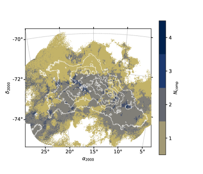
Figure 2: Map of total number of significant Hi components ($N_{\rm comp}$), masked as described in Section 2.1. White contours denote $N({\rm HI})$ at levels of $[15,35,55,75,95,115]\times 10^{20}\rm\,cm^{-2}$.

2.1 Neutral gas

As the SMC is rich in neutral atomic gas (e.g., Leroy et al., 2007), we use Hi to trace the gas distribution. New observations of the SMC at $21\rm\,cm$ were recently obtained by the Australian Square Kilometer Array Pathfinder (ASKAP; DeBoer et al., 2009) during Commissioning and Early Science observations in November 2017. These data were combined with single-dish observations of the SMC from the Parkes Telescope as part of the HI4Pi survey (HI4PI Collaboration et al., 2016). For details concerning the observations and data reduction for the ASKAP+Parkes cube, we refer the reader to McClure-Griffiths et al. (2018). The final data cube we use has a root mean square (RMS) noise in $21\rm\,cm$ brightness temperature ($T_{B}$) of $\sigma_{T_{B}}=0.7\rm\,K$, a pixel size of $7^{\prime\prime}$ ($35^{\prime\prime}\times 27^{\prime\prime}$ angular resolution), and velocity channel width of $3.9\rm\,km\,s^{-1}$ (McClure-Griffiths et al., 2018; Di Teodoro et al., 2019). For comparison with stellar velocities, we convert the Hi velocities from the Local Standard of Rest to the Heliocentric reference frame. Hereafter, all quoted velocities will be in the Heliocentric reference frame.

In Figure 1 we display a map of the Hi column density ($N({\rm HI})$) of the SMC from the ASKAP+Parkes data cube (panel a), the first moment map (panel b), and a position-velocity slice along the major axis inferred from kinematic modeling of the Hi data cube by Di Teodoro et al. (2019) (panel c, see Section 2.4). The moment map is masked as in Di Teodoro et al. (2019), wherein a flood-fill algorithm applied to a smoothed version of the data cube (smoothed with Gaussian kernel of FWHM $70^{\prime\prime}$) identified pixels with emission brighter than $\sim 10\sigma_{\rm HI}$, out to pixels with $\sim 4\sigma_{\rm HI}$ (where $\sigma_{\rm HI}$ is the RMS of the smoothed data).

2.2 Stars

We select a sub-sample of SMC stars with measured radial velocities from the spectroscopic survey of the SMC by the 2-degree-field instrument at the Anglo-Australian Telescope (2045 stars; Evans & Howarth, 2008) and from the Runaways and Isolated O-Type Star Spectroscopic Survey of the SMC (RIOTS4), a uniformly selected survey of young field stars in the SMC using the Inamori-Magellan Areal Camera and Spectrograph (IMACS) and Magellan Inamori Kyocera Echelle (MIKE) on the Magellan telescopes (374 stars; Lamb et al., 2016). Of this sample, 1484 stars are of spectral type O or B and have significant radial velocity ($v_{r}$) measurements (defined as $v_{r}/\sigma_{v_{r}}>5$, where $\sigma_{v_{r}}$ is the uncertainty on the radial velocity measurement).

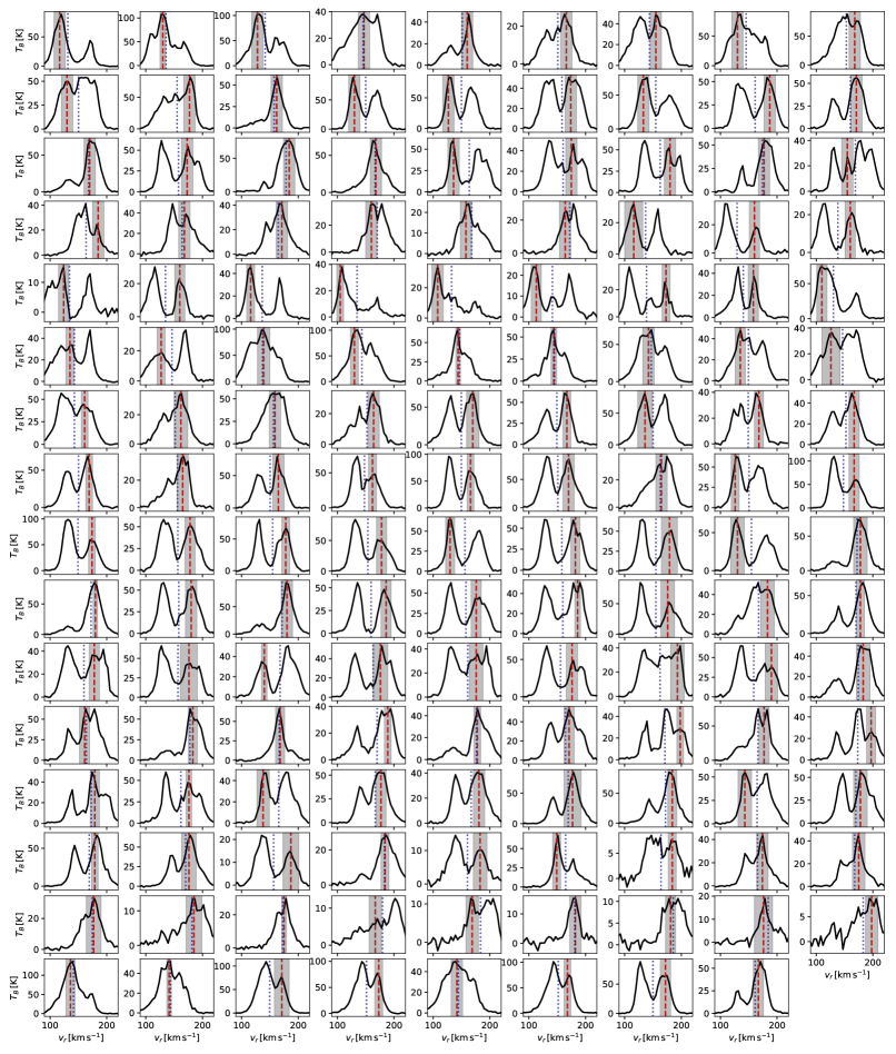
Figure 3: Results of matching observed radial velocities of young, massive stars (red dashed) with the radial velocities of distinct Hi peaks along the same LOS (black). For each of the $1202$ stars with radial and transverse velocity measurements, over 1000 trials we sample random velocities within $\pm 1\sigma_{v}$ (grey) and find the $143$ LOS which “match” (see Section 3.2). The $\pm 1\sigma$ uncertainties on the $v_{r,\rm star}$ are illustrated (grey shading), and the first moment (Figure 1b) is included (blue dotted).

To determine the transverse velocities of the selected stars, we cross-match them with SMC stars from the second data release (DR2) of the Gaia mission (Gaia Collaboration et al., 2018). The targets observed by Evans & Howarth (2008) and Lamb et al. (2016) are selected from the original catalog by Massey (2002), who reported a positional uncertainty of $1^{\prime\prime}$ per target. We begin with a conservative search radius of $3\sigma$ and find unique 1451 Gaia sources within $3^{\prime\prime}$ of the selected stars. All matched targets have significant PM ($\mu$) detections in right ascension ($\alpha$) and declination ($\delta$) ($\mu_{\alpha}/\delta_{\mu_{\alpha}}>5$ and $\mu_{\delta}/\delta_{\mu_{\delta}}>5$ where $\delta_{\mu_{\alpha}}$ and $\delta_{\mu_{\delta}}$ are the uncertainties in RA and Dec proper motions respectively). The matched stars represent the youngest, brightest end of the population observed by Gaia; for example, the median Gaia $G$ magnitude for the matched sample is $G=15.3$, compared with the median magnitude for the full SMC sample of $G=19$. We further refine the sample by comparing the observed flux densities, and remove $249$ objects with discrepant $G-B$ colors (defined as being further from the mean $G-B$ color of $0.16$ by more than $\pm 1\sigma=0.47$). The final sample contains $1202$ sources.

2.3 Systemic proper motion

To estimate the PMs due to internal motions of the SMC, we subtract the systemic motion of the galaxy from the measured Gaia PMs. For consistent comparison with the latest dynamical modeling of the system (see Section 2.4), we adopt the measured center of mass (COM) PM derived from HST photometry by Kallivayalil et al. (2013), who estimated $\mu_{W,0}=-0.772\pm 0.063\,\rm mas\,yr^{-1}$ and $\mu_{N,0}=-1.117\pm 0.061\,\rm mas\,yr^{-1}$. We note that many studies have estimated the COM PM of the SMC (e.g., Piatek et al., 2008; Kallivayalil et al., 2013; van der Marel & Sahlmann, 2016; Zivick et al., 2018; Niederhofer et al., 2018), and all estimates are largely consistent within uncertainties.

2.4 Dynamical model

For comparison with the observed kinematics, we use the results of a recent dynamical model in the SMC by Di Teodoro et al. (2019, hereafter dT19) based on the ASKAP+Parkes Hi data cube. dT19 modeled the SMC as a disk undergoing circular rotation. Using a Markov Chain Monte Carlo (MCMC) approach, they fitted the observed velocity field (e.g., Figure 1b) to derive global properties of the system, including kinematic center, position and inclination angles, transverse and systemic velocities, and then applied a tilted-ring analysis to decompose the velocity field and extract the rotation velocity as a function of radius.

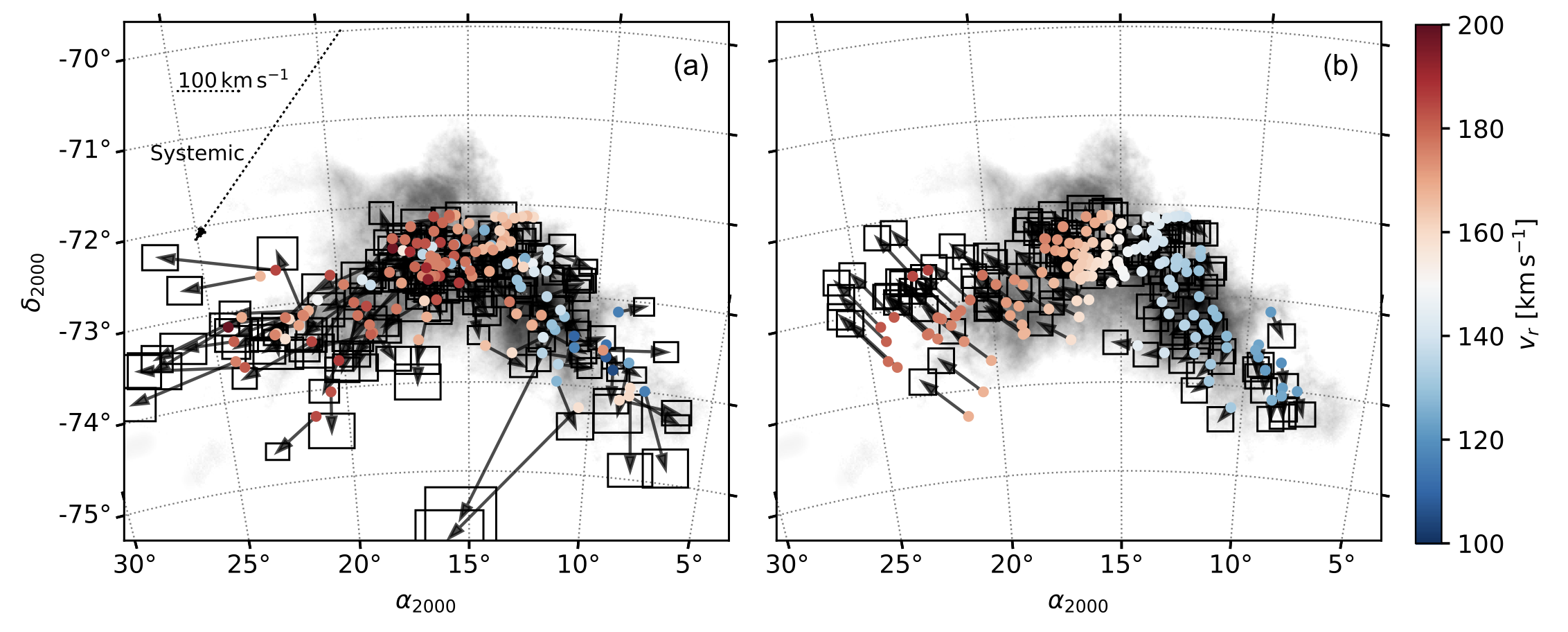
Figure 4: (a): Radial velocities (color) and residual PMs (vectors) for the sample of $143$ stars with significantly-detected radial and transverse motions from spectroscopy (Evans & Howarth, 2008; Lamb et al., 2016) and Gaia (Gaia Collaboration et al., 2018), whose radial velocities match significant Hi components along the line of sight (c.f. Figure 3). All vectors are constructed to illustrate PMs over the next $7.2\rm\,Myr$ (arbitrarily, as in van der Marel & Sahlmann, 2016). The systemic PM of the SMC (Kallivayalil et al., 2013) is included at top left (dotted), as is a scale bar to illustrate $100\rm\,km\,s^{-1}$ (dashed). (b) Same, for the predicted radial velocities and residual PMs (black vectors) from the SMC rotation model by dT19.

Using the dT19 results, we predict the velocities for stars within a rotating SMC based on their coordinates. To compute each velocity component, we follow van der Marel & Cioni (2001, hereafter vdM2001) and van der Marel et al. (2002, hereafter vdM2002). We assume the same global SMC parameters as derived in the dT19 model, including: the SMC COM ($\alpha_{0,2000}=15.237\pm 0.380^{\circ},\,\delta_{0,2000}=-72.273\pm 0.290^{\circ}$), distance ($D_{0}=63\pm 5\rm\,kpc$), COM PM ($\mu_{W,0}=-0.772\pm 0.063,\,\mu_{N,0}=-1.117\pm 0.061\,\rm mas\,yr^{-1}$; Kallivayalil et al., 2013), systemic LOS velocity (Heliocentric, $v_{r,\rm sys}=157\pm 2\rm\,km\,s^{-1}$), inclination ($i=55\pm 9^{\circ}$), position angle of the line of nodes ($\rm PA=66\pm 8^{\circ}$; measured counter-clockwise from North) and precession and nutation rate ($\partial i/\partial t=-281\pm 100\rm\,^{\circ}/Gyr$). From the assumed COM PM, we also compute the transverse velocity of the COM and its angle on the sky.

Given these global parameters, for each star, we compute its angular coordinates on the sky (Equations 1-3; vdM2001), its radius in the galaxy frame (Equation 9; vdM2002), and its ensuing predicted rotation velocity from the dT19 model. We then follow vdM2002 to compute the individual velocity contributions from the SMC COM (Equation 13), its precession and nutation (Equation 16) and internal motions (Equation 21). The sum of these components comprise the predicted velocities in the frame of the SMC. Finally, we extract the predicted radial velocity ($v_{r,\rm Model}$), and the PMs to the West and North ($\mu_{W,\rm Model},\,\mu_{N,\rm Model}$; Equation 9; vdM2002) for comparison with the observed sample. As an estimate of the uncertainties in these predictions, we propagate the quoted uncertainties in the nine global SMC parameters from dT19 through the analysis.

3 Analysis

3.1 Line of Sight Complexity

Although the radial velocity structure of Hi in the SMC is complex, it has been shown that a significant fraction of OB stars have coincident radial velocities with Hi structures along the same LOS, and are therefore embedded within the Hi distribution (Lamb et al., 2016). Although the majority of young stars are associated with some Hi emission, our goal is to construct a pure sample of targets which are most likely to trace the motions of dominant Hi components.

We begin by identifying significant Hi components along each line of sight in the ASKAP+Parkes data cube via the derivative of $T_{B}(v_{r})$. First, we re-sample each $T_{B}(v_{r})$ spectrum to $0.5\rm\,km\,s^{-1}$ resolution and smooth with a Gaussian kernel of width $8$ channels to suppress the influence of noise on selecting spurious peaks. We then compute the first numerical derivative of each spectrum and identify components as local maxima with significant emission ($T_{B}>5\rm\,K$). Figure 2 displays the total number of significant Hi components along each LOS. Although the outskirts of the SMC typically feature a single strong Hi component, within the main body of the SMC the radial velocity structure of the gas is more complex and there are at least two Hi components. This is evident in Figure 1c: in addition to the “main disk” of the SMC along the major axis inferred by rotation models, there are several significant velocity components evident in the position-velocity diagram.

3.2 Matching radial velocities

To identify which stars are moving with the identified Hi components, we compare the observed stellar radial velocities ($v_{r,\rm star}$) with the radial velocities of the Hi components ($v_{r,\rm HI}$). To select the most likely sources to trace the dominant Hi along each line of sight, we design a method for matching stars with Hi components which accounts for the uncertainties in $v_{r,\rm star}$, which can be large ($\sigma_{v_{r,star}}\sim 5-30\rm\,km\,s^{-1}$; Evans & Howarth, 2008; Lamb et al., 2016).

For each star, we select $N=1000$ velocities distributed normally with mean $v_{r,\rm star}$ and $\sigma=\sigma_{v_{r,\rm star}}$. For each Hi component, we construct similar normally-distributed velocity distributions with mean $v_{r,\rm HI}$ and an assumed $\sigma=\sigma_{\rm HI}\rm\,km\,s^{-1}$. We then use a two-sample Anderson-Darling test (A-D; Anderson & Darling, 1954) to test for the null hypothesis that the stellar and Hi velocity distributions are drawn from the same parent population. A match is achieved if the null hypothesis cannot be rejected with high confidence ($>99\%$), and if the brightness temperature of the Hi peak is above a certain fraction of the max $T_{B}$ along the line of sight ($r_{\rm peak}$, where $r_{\rm peak}=T_{B,\rm peak}/\max({T_{B}(v_{r})})$), to ensure that matches are with dominant Hi peaks.

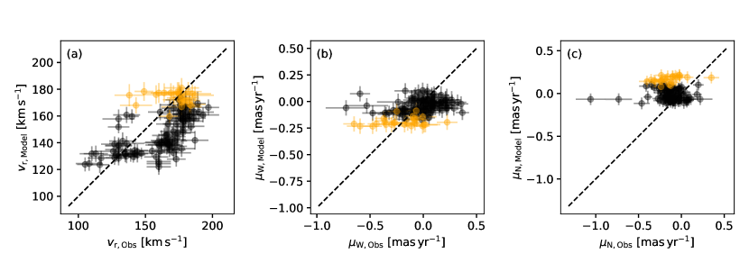
Figure 5: Comparison between radial velocity ($v_{\rm r}$) and PMs to the West and North ($\mu_{W}$ and $\mu_{N}$) observed (“Obs”) and predicted by dT19 (“Model”) for the sample of $143$ stars whose radial velocities match significant Hi components. The error bars on $v_{r,\rm Obs}$ are $1\sigma$ uncertainties (Evans & Howarth, 2008; Lamb et al., 2016), and the error bars on $\mu_{W,\rm obs}$ and $\mu_{N,\rm obs}$ are $1\sigma$ uncertainties from the Gaia DR2 catalog (Gaia Collaboration et al., 2018). The error bars for the “Model” parameters are estimated by propagating the uncertainties in the global SMC parameters through the velocity calculations (see Section 2.4). We divide the sample by location in the SMC (see Figure 1a for definitions): the Bar (black), and Wing (orange).

To select the optimal values for the matching parameters ($\sigma_{\rm HI}$ and $r_{\rm peak}$), we repeat the match process for a range of values ($1<\sigma_{\rm HI}<10\rm\,km\,s^{-1},\,0<r_{\rm peak}<1$), and select the values which maximize the number of matches while minimizing the contamination fraction. To quantify the contamination of the sample due to random interlopers with coincidental radial velocities to the Hi peaks, we repeat the matching process using simulated samples of $1202$ stars with random velocities and uncertainties drawn from the observed distributions over 1000 trials. The estimated number of spurious matches is computed as the median over all trials. We find that the choice of $\sigma_{\rm HI}$ and $r_{\rm peak}$ does not have a significant effect on the results, and the contamination fraction is $\sim 25\%$ for all tested values. We will discuss the effect of this contamination fraction in Section 4. We select $\sigma_{\rm HI}=5\rm\,km\,s^{-1}$ and $r_{\rm peak}=0.3$.

We note that this approach produces statistically indistinguishable results from other methods of matching $v_{r,\rm star}$ and $v_{\rm HI}$, including: (1) by-eye matching, (2) applying a range of absolute cuts to $\Delta v_{r}=|v_{r,\rm star}-v_{r,\rm HI}|$, and (3) computing the area of overlap between the $v_{r,\rm star}$ and $v_{r,\rm HI}$ distributions and applying a sigma cut.

To determine the final sample, we repeat the matching process with the selected match criteria over an additional 1000 trials, and select all stars which are successful matches in more than $95\%$ of trials. The result is a sample of $143$ stars. The matched sources are shown in Figure 3. In the Appendix, we include similar figures for all LOS (Figures 6 through 14).

Although the final sample represents only $\sim 12\%$ of the initial sample of stars with both radial and transverse velocity constraints ($1202$ sources), this does not mean that the remaining $88\%$ of the sample are not associated with Hi gas. In fact, we observe that the majority of the initial sample of $1202$ stars ($\sim 80\%$) is associated with significant Hi emission, defined has there being significant Hi emission at the radial velcoity of the star ($T_{B}(v_{r,\rm star})>5\rm\,K$). This indicates that most stars are embedded somewhere within the neutral gas distribution, if not associated with the strongest peeaks. The final sample of $143$ matched stars represents our highest confidence for tracing the Hi kinematics with minimal contamination. We further observe that although relaxing the matching criteria (e.g., including wider uncertainty ranges, selecting different brightness temperature cuts to define Hi components, etc) changes the number and selection of stars which are included in the matched sample, it does not significantly affect the statistics of the sample (e.g., estimated contamination fraction) or the ensuing conclusions.

4 Results

In Figure 4a we display the residual PMs (i.e., with the COM PM from Kallivayalil et al. (2013) subtracted) for the $143$ stars whose radial velocities match with significant Hi peaks. The stars exhibit a radial velocity gradient in agreement with the Hi radial velocity field (Figure 1b). However, the observed residual PMs do not exhibit a clear signature of rotation. For comparison, in Figure 4b, we display the radial velocities and residual PMs predicted by the dT19 rotation model. As expected, the modeled residual PMs exhibit a clear signature of rotation.

Comparing the panels of Figure 4, although the observed and modeled kinematics are not consistent throughout the SMC, the level of agreement may depend on location within the system. For example, a subset of stars have large observed tangential velocities ($\sim 100\rm\,km\,s^{-1}$). These large velocities are likely dominated by dynamical effects (Oey et al., 2018). Stars in the the Wing region (Southeast, c.f. Figure 1a) are moving towards the LMC via the Magellanic Bridge as a result of their recent interaction history (Zivick et al., 2019). Furthermore, this net PM of the Wing relative to the Bar indicates that these two regions may be kinematically distinct (Oey et al., 2018). Although stars and gas throughout the SMC are affected at some level by the same dynamical interactions, in subsequent analysis we will distinguish stars in the Wing and Bar to account for the possibility that stars in different regions are tracing distinct populations.

In Figure 5 we compare the observed and predicted radial (LOS) velocity (a), and the residual PMs to the West and North (b and c) for the $143$ matched stars. Stars located in Wing and Bar are distinguished from each other for clarity (see Figure 1a for definitions).

Figures 4 and 5 indicate that the observed kinematics are largely inconsistent with the predictions from the rotating disk model. To quantify the agreement, we use the K-sample A-D statistic. First, we bootstrap the sample with replacement over 1000 trials, and within each trial use a simple Monte Carlo exercise to draw random values of each velocity component within $\pm 3\sigma$ to compute the A-D statistic. The final value is a median over all trials. We find that the null hypothesis that the observed and modeled velocity distributions are drawn from the same parent population is ruled out with $>99\%$ confidence for $v_{r}$, $\mu_{W}$ and $\mu_{N}$ for the full sample. When treating the two regions of the SMC separately, the agreement does not improve significantly: the null hypothesis is ruled out in all cases with $>99\%$ confidence again, with the exception of the radial velocity of the Wing ($98\%$ confidence). To explicitly and conservatively account for the estimated $25\%$ contamination from random interlopers, we repeat the above exercise and exclude the worst $25\%$ in each trial (defined as those points with the largest absolute difference between observed and modeled velocities). We find consistent results as for the full sample (agreement ruled out with $>99\%$ confidence, despite some improvement in the Bar and Wing sub-samples) except for the cases of $\mu_{W}$ for the full sample ($98\%$ confidence).

5 Discussion

Overall, the observed 3D kinematics of Hi in the SMC traced by young massive stars are inconsistent with predictions from the rotating disk model. In the following, we discuss how to reconcile this result within the context of the SMC.

First, it is important to consider alternatives to the hypothesis that the SMC is well-represented by a single rotating disk. As discussed by dT19, there are several caveats to the disk model, including the fact that the disk is not razor-thin (as must be assumed to simplify the velocity component computation), the rotation is not necessarily perfectly circular and the disk is not necessarily axisymmetric. In addition to these caveats, there is clear evidence that significant components of the system (e.g., the Wing) are dominated by radial motions due to the influence of the LMC (e.g., Zivick et al., 2019). The fact that the rotation model performs as well as it does at reproducing the radial velocity field of the gas suggests that the large scale motion is dominated by rotation, and the discrepant stellar kinematics observed here may reflect only local, non-circular motions. Although a subset of our sample likely does trace local motions (e.g., effects of stellar feedback on small scales), the majority were selected to trace the dominant Hi components. As seen in Figure 5a, the observed radial velocities of stars matched to Hi peaks trace distinct, coherent components in radial velocity, one at $\sim 130\rm\,km\,s^{-1}$ and one at $\sim 160\rm\,km\,s^{-1}$, which are found in both the Wing and the Bar. The intensity-weighted mean velocity along each LOS used to predict 3D gas motions can be insensitive to this multiplicity, especially if there are multiple components with similar intensities. To illustrate this effect, in Figure 3, we include the first moment for comparison with the Hi peak velocities along each LOS. In addition, we note that although Gaia PMs in the SMC display a marginal signal of rotation (Gaia Collaboration et al., 2018, Figure 16), it is inconsistent with the rotation inferred from the Hi.

An alternative explanation for the discrepancy between the observed and model kinematics is that the SMC is not a single system, but is rather composed of multiple structures along the LOS. As illustrated in Figure 2 and Figure 5, the structure of the SMC is complex, and exhibits multiple, significant Hi components separated in radial velocity. This velocity structure has previously been attributed to separate sub-systems within the SMC (e.g., the Mini Magellanic Cloud and the SMC Remnant; Mathewson & Ford, 1984), which may be separated in distance along the LOS by $>10\rm\,kpc$ (Mathewson et al., 1986). Based on measurements of UV absorption lines towards stars in the SMC, the lower-velocity Hi component appears to be sitting in front of the higher-velocity Hi component along the LOS (Songaila et al., 1986; Wayte, 1990; Danforth et al., 2002; Welty et al., 2012). This implies that the SMC is being ripped apart by its interactions with the LMC, in agreement with tidal models of the system (Murai & Fujimoto, 1980), resulting in disparate remnant structures.

If the SMC is composed of separate sub-systems at different distances, it is possible that the apparent rotation seen in the radial velocity field of the gas is dominated by rotation within one component over the other. However, exactly how we can reconcile potential rotation in this component alone with the non-rotating kinematics of the rest of the SMC is uncertain, and not incorporated into current theoretical models. In addition, it has been shown that models with purely radial motions can reproduce observed velocity fields just as well as disk models with purely rotational motion (e.g., Sylos Labini et al., 2019). Furthermore, the derived global properties of the system, including its dynamical center and mass — crucial input parameters to numerical models of the broader Magellanic System (Besla et al., 2012) — are based on fits to the global radial velocity field (e.g., including all velocities along each LOS; Figure 1). If only subsets of the SMC are actually rotating, these models (and the resulting parameters) would still need to be revisited.

6 Summary and Conclusions

In this paper, we present new constraints for the 3D kinematics of gas in the SMC. We trace the transverse motions of Hi in the system for the first time using the observed proper motions of massive, young stars whose radial velocities match with significant Hi components identified from new observations by the ASKAP telescope (McClure-Griffiths et al., 2018). We test the hypothesis that gas in the SMC is rotating in a disk by comparing the observed radial and transverse velocities of young stars with predictions from the latest model of the radial velocity field from dT19. Our main conclusions are the following:

• The observed motions of gas-tracing stars are inconsistent with the predictions from the dT19 rotation model, even when the contamination from random interlopers is explicitly taken into account (Figures 4, 5).

• The 3D kinematics of the SMC are more complex than can be accurately inferred from the integrated radial velocity field alone.

• Due to violent tidal and ram-pressure interactions with the LMC and the MW halo, it is likely that the SMC is composed of overlapping sub-structures, whose properties should be considered in future models of the system for extracting basic parameters such as the COM, dynamical mass and depth along the LOS.

Overall, this study represents one step in the process of unraveling the structure and kinematics of the SMC. In the near future, with the third data release from Gaia, we will have access to radial velocity measurements towards a new sample of stars throughout the SMC with which we will further dissect the kinematics of individual gaseous components. In addition, with resolved stellar photometry, we will constrain the distances to individual dusty components and complete the full 6D phase space of the system (3D positions, 3D velocities). As the Magellanic Clouds are the only systems for which we can achieve this level of resolution, this will not only inform our understanding of these systems, but also our understanding of dwarf galaxy interactions throughout cosmic time.

Appendix A Matching radial velocities

In this Appendix, we provide supplemental figures and tables for illustrating the match process between the observed radial velocities of young, massive stars (Evans & Howarth, 2008; Lamb et al., 2016), and the observed radial velocities of significant Hi peaks along the same LOS. In Figures 6 through 14 we display plots for each of $1202$ stars with significant radial velocities with corresponding proper motion measurements from Gaia DR2 (Gaia Collaboration et al., 2018). We include the Hi spectrum ($T_{B}(v_{r})$) and the identified significant components along each LOS. The $143$ matched LOS are identified by purple plot frames (and are also shown in Figure 3).

In Table A, we include the coordinates, velocities, and proper motions for the $143$ Hi-matched stars.

Figure 6: Each panel compares the $21\rm\,cm$ $T_{B}(v_{r})$ spectrum and identified Hi components ($v_{r,\rm HI}$; dotted green) with the observed stellar radial velocity ($v_{r,\rm star}$; red dashed). The uncertainties in $v_{r,\rm star}$ are illustrated by 50 random draws from a normal distribution with $\mu=v_{r,\rm star}$ and $\sigma=\sigma_{v_{r,\rm star}}$ (grey). The $143$ matches (see text) are highlighted by bold, purple plot frames (also see Figure 3). If $v_{r,\rm star}$ is not visible within the panel, it falls outside the plotted velocity range.

Figure 7: See Figure 6.

Figure 8: See Figure 6.

Figure 9: See Figure 6.

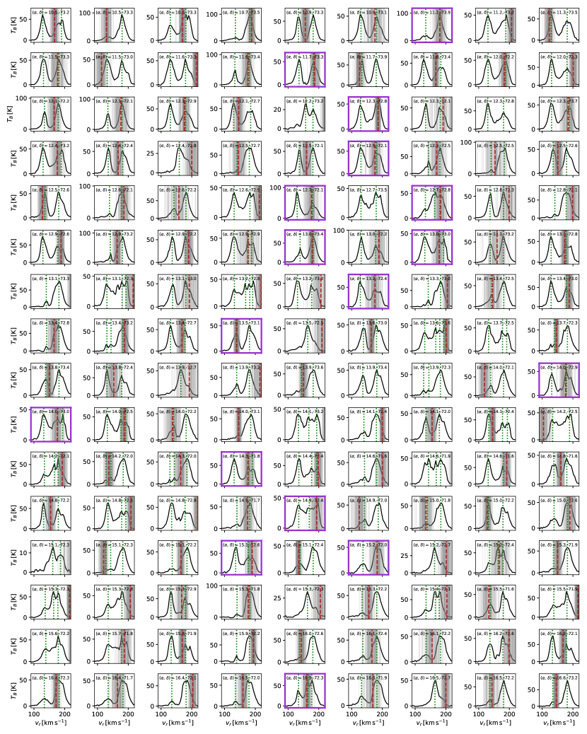
Figure 10: See Figure 6.

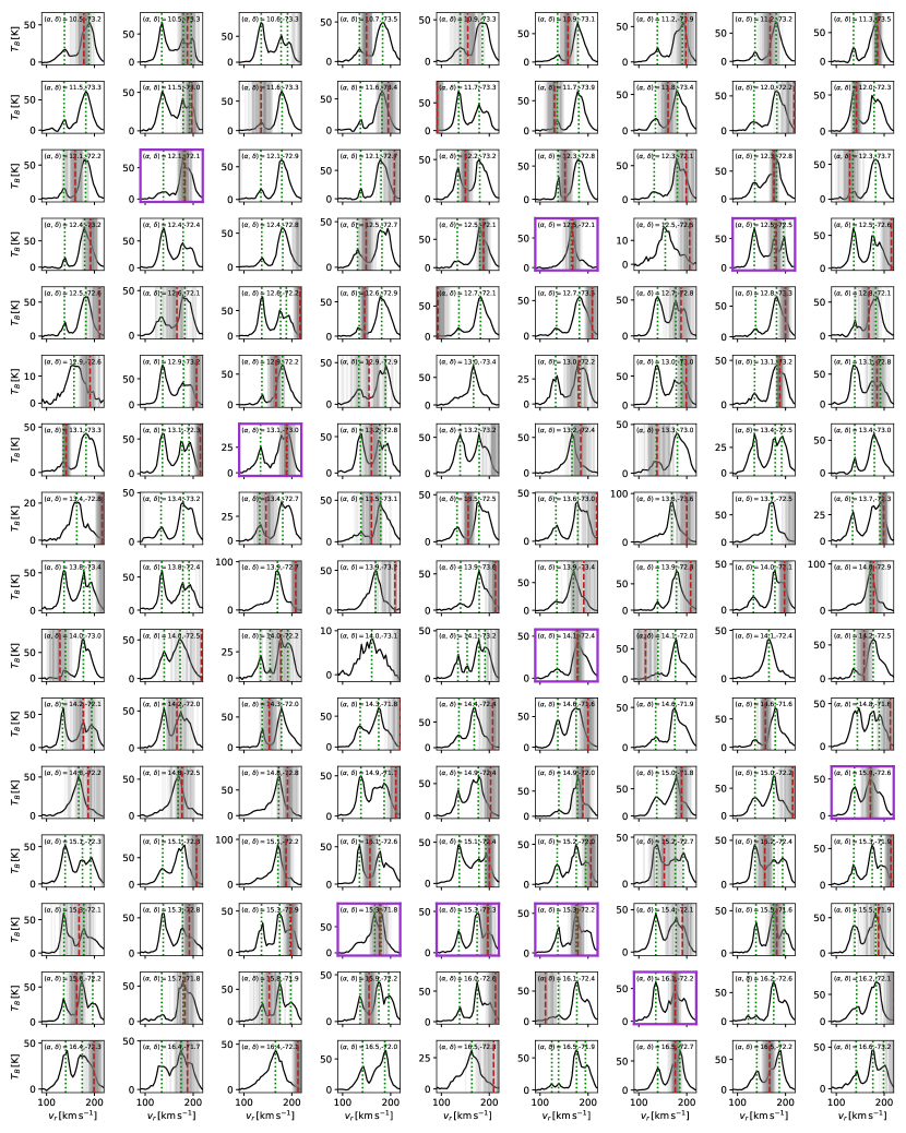
Figure 11: See Figure 6.

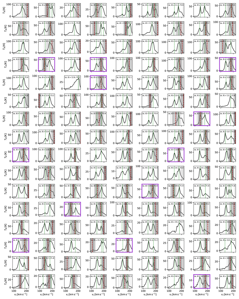
Figure 12: See Figure 6.

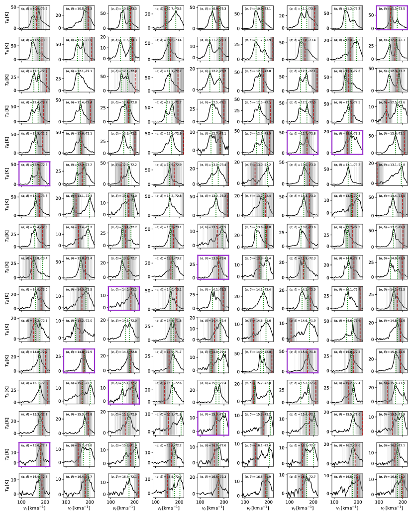
Figure 13: See Figure 6.

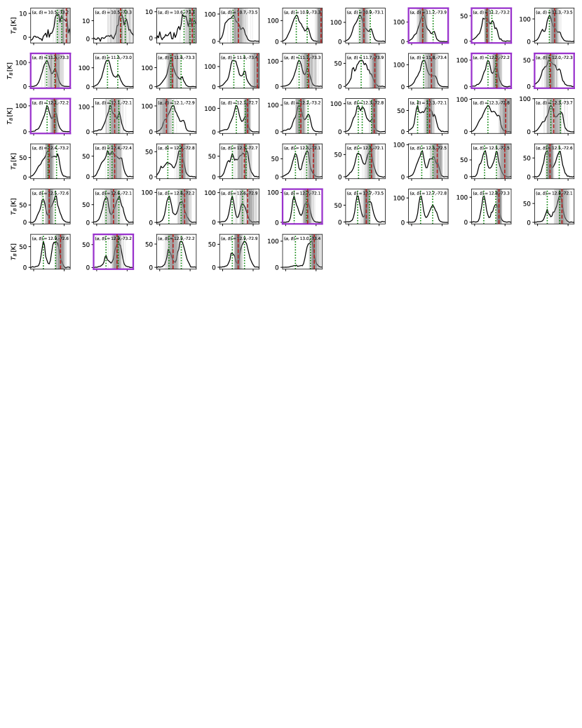
Figure 14: See Figure 6.

Table 1: Parameters for the $143$ stars used in the kinematic comparison. (1-2): RA, Dec coordinates; (3-4): Observed radial velocity and uncertainty; (5) Stellar type; (6) Radial velocity reference, 1=Lamb et al. (2016), 2=Evans & Howarth (2008); (7-10): Proper motions and uncertainties in the West (7,9) and North (8,10) directions from Gaia Collaboration et al. (2018).

RA	Dec	$v_{r,\rm star}$	$\delta{v_{r,\rm star}}$	Type	Ref	$\mu_{W}$	$\mu_{N}$	$\delta{\mu_{W}}$	$\delta{\mu_{N}}$
(deg)		($\rm km\,s^{-1}$)				($\rm mas\,yr^{-1}$)
(1)	(2)	(3	(4)	(5)	(6)	(7)	(8)	(9)	(10)
7.798	-73.993	116.0	16.0	B1-3 (V)	2	-0.656	-1.550	0.127	0.107
8.410	-73.973	160.0	9.0	B1-3 (IV)	2	-0.772	-1.580	0.125	0.092
8.412	-74.064	160.0	9.0	B9 (Ib)	2	-0.501	-1.274	0.067	0.050
8.565	-73.694	124.0	9.0	B3-5 (III)	2	-0.834	-1.402	0.136	0.107
8.793	-74.122	160.0	9.0	B9 (II)	2	-0.450	-1.190	0.082	0.069
9.178	-73.137	116.0	7.0	B8 (II)	2	-0.628	-1.088	0.056	0.049
9.178	-73.794	105.0	6.0	B8 (II)	2	-0.782	-1.291	0.097	0.069
9.504	-73.652	108.0	10.0	B9 (Ib)	2	-0.593	-1.219	0.047	0.043
9.536	-73.516	113.0	9.0	B9 (II)	2	-0.712	-1.269	0.055	0.051
9.641	-73.579	173.0	7.0	B1-3 (II)	2	-0.418	-1.128	0.068	0.056
10.452	-74.245	158.0	9.0	B0.5 (V)	2	-1.498	-1.849	0.191	0.154
10.793	-73.575	117.0	10.0	B1.5e3+	1	-0.619	-1.062	0.076	0.065
10.826	-73.446	110.0	9.0	B5 (III)	2	-0.554	-1.242	0.061	0.058
11.258	-73.234	130.0	5.0	B0 V	1	-0.692	-1.213	0.066	0.067
11.393	-73.773	135.0	7.0	B8 (II)	2	-0.596	-1.139	0.068	0.056
11.419	-73.965	127.0	7.0	B1-2 (II)	2	-0.668	-1.371	0.102	0.074
11.429	-73.163	139.0	11.0	B9 (II)	2	-0.673	-1.007	0.067	0.059
11.594	-73.388	128.0	10.0	O9.5-B0 III	1	-1.303	-2.176	0.200	0.174
11.732	-73.332	130.0	7.0	B9 (Ib)	2	-0.846	-1.053	0.049	0.043
11.981	-73.020	136.0	8.0	B8 (II)	2	-0.583	-1.048	0.074	0.047
12.002	-72.570	144.0	4.0	B1-2 (III)	2	-0.606	-1.244	0.078	0.061
12.014	-72.500	144.0	5.0	B9 (Ib)	2	-0.547	-1.209	0.050	0.040
12.039	-72.730	141.0	4.0	B1-2 (II)	2	-0.737	-1.147	0.057	0.047
12.050	-73.480	142.0	10.0	B0-5 (II)	2	-0.798	-1.243	0.068	0.065
12.060	-73.657	135.0	9.0	B2.5 (Ib)	2	-0.552	-1.152	0.055	0.046
12.159	-73.232	171.0	13.0	B1-5 (II)	2	-0.770	-1.265	0.074	0.056
12.495	-73.345	173.0	7.0	B0 (IV)	2	-0.486	-1.271	0.074	0.063
12.503	-72.747	142.0	10.0	B1-5 (III)	2	-0.731	-1.032	0.073	0.062
12.520	-73.351	168.0	6.0	B0.5 (V)	2	-0.620	-1.026	0.078	0.069
12.580	-72.655	147.0	10.0	B0 V	1	-0.506	-1.214	0.090	0.066
12.607	-72.134	160.0	10.0	O9.5 V	1	-0.778	-1.330	0.086	0.064
12.846	-72.122	166.0	10.0	B1 I	1	-0.941	-1.211	0.101	0.064
12.875	-72.599	126.0	16.0	B1-5 (III)	2	-0.562	-1.046	0.073	0.061
12.927	-72.698	161.0	6.0	B1-3 (II)	2	-1.009	-0.897	0.198	0.143
12.931	-72.624	155.0	10.0	B1 II	1	-0.565	-1.190	0.055	0.044
12.999	-72.923	130.0	10.0	Be3	1	-0.867	-1.119	0.066	0.047
13.035	-72.134	162.0	12.0	B0 (II)	2	-0.734	-1.201	0.068	0.051
13.129	-73.227	168.0	10.0	O9-B0 pe3+	1	-0.747	-1.087	0.060	0.040
13.148	-72.847	130.0	10.0	B1.5e3+	1	-0.755	-1.178	0.060	0.044
13.267	-73.666	159.0	10.0	B5 (II)	2	-0.405	-0.934	0.063	0.055
13.304	-72.151	164.0	10.0	B0 (V)	2	-0.818	-1.255	0.092	0.067
13.361	-72.641	170.0	11.0	B0 (III)	2	-0.727	-1.263	0.083	0.051
13.415	-73.094	177.0	10.0	B0.5 III	1	-0.538	-1.142	0.103	0.058
13.434	-72.416	167.0	7.0	B1-5 (II)	2	-0.691	-1.304	0.070	0.062
13.528	-72.667	136.0	13.0	B1-5 (III)	2	-0.697	-1.264	0.088	0.071
13.584	-72.219	168.0	8.0	B0.5 (IV)	2	-0.911	-1.145	0.090	0.070
13.671	-72.344	167.0	9.0	B1-5 (II)	2	-0.750	-1.351	0.060	0.056
13.745	-72.419	169.0	6.0	B5 (II)	2	-0.696	-1.182	0.059	0.055
13.748	-72.146	165.0	10.0	B8 (II)e?	2	-0.666	-1.247	0.080	0.065
13.790	-72.465	165.0	10.0	B1-3 (II)	2	-1.367	-1.143	0.094	0.077
13.840	-72.296	162.0	7.0	B3 (II)	2	-0.810	-1.312	0.058	0.054
14.007	-72.140	162.0	10.0	O8 V	1	-0.879	-1.391	0.081	0.064
14.058	-72.500	130.0	10.0	B0.5e1	1	-0.825	-1.283	0.048	0.047
14.080	-72.515	172.0	9.0	B1-5 (II)	2	-0.770	-1.208	0.062	0.060
14.135	-72.464	127.0	10.0	Be4+	1	-0.860	-1.295	0.070	0.068
14.200	-72.479	166.0	6.0	B1-3 (II)	2	-0.672	-1.231	0.059	0.058
14.206	-72.755	170.0	10.0	B0.5 (IV)	2	-0.693	-1.261	0.065	0.057
14.335	-73.590	165.0	10.0	B0-5 (II)	2	-0.557	-1.232	0.076	0.062
14.406	-72.292	126.0	7.0	B8 (II)	2	-1.132	-1.398	0.096	0.072
14.464	-72.508	167.0	9.0	B2 (II)	2	-0.765	-1.237	0.065	0.053
14.732	-72.535	174.0	6.0	B0 (Ib)	2	-0.559	-1.169	0.064	0.057
14.864	-72.810	174.0	10.0	O8.5 V	1	-0.736	-1.268	0.086	0.064
14.941	-72.749	178.0	9.0	B0 (Iab)	2	-0.688	-1.316	0.065	0.055
14.979	-72.218	167.0	9.0	B9 (Ib)	2	-0.881	-1.227	0.054	0.039
15.071	-72.397	178.0	7.0	B0.5 (V)	2	-0.818	-1.189	0.076	0.059
15.085	-72.690	133.0	10.0	B0 III	1	-0.703	-1.509	0.060	0.051
15.116	-72.648	178.0	9.0	B0-5 (III)	2	-0.701	-1.156	0.105	0.073
15.358	-72.885	187.0	10.0	B1.5 III	1	-0.608	-1.304	0.070	0.051
15.387	-72.279	171.0	10.0	O6 V	1	-0.996	-1.074	0.094	0.065
15.479	-72.124	170.0	10.0	O7 III((f))e1	1	-0.825	-1.143	0.080	0.069
15.504	-72.453	130.0	8.0	O8.5 III((f))	2	-0.961	-1.280	0.077	0.060
15.541	-72.584	182.0	8.0	O9.5 III	2	-0.822	-1.213	0.079	0.071
15.548	-72.457	179.0	14.0	B0.5 (V)	2	-0.947	-1.361	0.082	0.062
15.662	-72.668	130.0	12.0	B1-5 (II)	2	-0.659	-1.240	0.077	0.063
15.693	-72.153	178.0	12.0	B2 (IV)	2	-0.851	-1.266	0.106	0.077
15.699	-72.122	180.0	4.0	B8 (Ib)	2	-0.856	-1.249	0.055	0.041
15.884	-72.654	180.0	10.0	B1-5 (III)	2	-0.794	-1.257	0.101	0.087
15.953	-72.207	180.0	10.0	B1-3 (III)	2	-0.970	-1.186	0.079	0.064
16.046	-72.428	186.0	9.0	B0-5 (III)	2	-1.024	-1.251	0.092	0.073
16.063	-72.693	176.0	9.0	B0-5 (II)	2	-0.654	-1.256	0.078	0.057
16.097	-72.807	186.0	5.0	B1-3 (III)	2	-0.741	-1.141	0.061	0.053
16.222	-72.676	173.0	10.0	O8.5 V	1	-0.676	-1.121	0.074	0.064
16.227	-72.608	176.0	12.0	B1-5 (III)	2	-0.866	-1.378	0.118	0.092
16.240	-73.071	183.0	12.0	B9 (Ib)	2	-0.887	-1.126	0.055	0.042
16.274	-72.135	184.0	10.0	O9.5 V	1	-0.704	-1.257	0.087	0.054
16.276	-72.300	178.0	7.0	B1-3 (III)	2	-0.922	-1.146	0.109	0.060
16.281	-72.805	178.0	9.0	O5 V((f))	2	-0.751	-1.321	0.072	0.065
16.320	-72.670	176.0	15.0	B0-3 (V)	2	-0.684	-1.229	0.108	0.089
16.364	-72.478	140.0	5.0	B1-5 (Ib)	2	-0.966	-1.248	0.081	0.056
16.419	-72.577	176.0	13.0	B1-3 (III)	2	-0.799	-1.285	0.083	0.056
16.431	-72.801	176.0	12.0	B1-5 (II)	2	-0.770	-1.150	0.071	0.063
16.490	-72.663	176.0	10.0	B2 (IV)	2	-0.941	-1.209	0.093	0.066
16.543	-72.840	193.0	12.0	B3 (II)	2	-0.731	-1.244	0.063	0.053
16.600	-72.708	190.0	11.0	B2 (V)	2	-1.132	-1.433	0.137	0.098
16.612	-72.435	183.0	12.0	B1-3 (III)	2	-0.967	-1.112	0.093	0.069
16.637	-73.262	168.0	10.0	B0e3	1	-0.825	-1.361	0.124	0.076
16.708	-73.080	161.0	9.0	B5 (III)	2	-0.999	-1.257	0.083	0.058
16.713	-72.556	136.0	10.0	O8.5 V	1	-1.093	-1.269	0.087	0.069
16.757	-72.799	175.0	10.0	B1.5e2	1	-0.669	-1.316	0.065	0.052
16.916	-72.430	183.0	8.0	B0 (V)	2	-0.949	-1.231	0.110	0.077
16.985	-73.516	168.0	8.0	B0-5 (V)	2	-0.777	-1.354	0.128	0.098
17.030	-72.693	180.0	10.0	B1.5e3	1	-0.718	-1.264	0.056	0.050
17.133	-72.240	177.0	10.0	O9.5 III	1	-0.786	-1.230	0.114	0.071
17.191	-72.523	189.0	6.0	B0-5 (II)	2	-1.055	-1.368	0.084	0.073
17.362	-72.384	178.0	6.0	B1-5 (II)e	2	-0.785	-1.336	0.078	0.064
17.451	-72.505	155.0	10.0	O9 V	1	-1.243	-1.336	0.096	0.085
17.561	-72.870	171.0	9.0	B1-3 (IV)	2	-1.122	-1.528	0.078	0.082
17.800	-72.369	198.0	6.0	O9.5 III	2	-0.846	-1.355	0.084	0.057
17.803	-73.159	177.0	9.0	B1-3 (III)	2	-0.838	-1.241	0.092	0.065
17.832	-72.475	197.0	8.0	B2.5 (II)	2	-0.836	-0.919	0.067	0.061
17.833	-72.366	179.0	8.0	O8 III	2	-0.933	-1.323	0.124	0.072
17.998	-72.743	176.0	5.0	B1-5 (III)	2	-1.248	-1.464	0.097	0.090
18.746	-72.872	138.0	11.0	B0-5 (IV)	2	-1.022	-1.257	0.102	0.093
18.782	-73.411	177.0	9.0	B1-5 (II)	2	-0.871	-1.243	0.084	0.064
18.864	-73.426	181.0	10.0	B2.5 (II)	2	-1.145	-1.209	0.084	0.061
18.886	-73.318	177.0	15.0	B1-5 (III)	2	-0.852	-1.358	0.126	0.074
18.958	-73.107	184.0	8.0	B3-5 (III)	2	-0.849	-1.279	0.114	0.091
19.055	-72.807	143.0	12.0	B1-5 (III)	2	-1.039	-1.518	0.108	0.093
19.320	-73.205	178.0	12.0	B1-3 (III)	2	-0.859	-1.422	0.096	0.069
19.433	-73.056	179.0	6.0	B0-5 (III)	2	-0.548	-1.433	0.097	0.067
19.771	-72.845	176.0	13.0	B9: (II)	2	-1.134	-1.355	0.096	0.074
20.209	-73.692	187.0	14.0	B3-5 (III)e	2	-0.854	-1.290	0.083	0.064
20.258	-72.727	184.0	7.0	B0.5 (V)	2	-1.121	-1.470	0.103	0.074
20.647	-74.035	183.0	12.0	B0-5 (IV)	2	-0.767	-1.337	0.128	0.097
20.813	-72.992	149.0	7.0	B1-5 (III)	2	-0.834	-1.314	0.112	0.094
21.213	-73.450	185.0	10.0	O8 V	1	-1.149	-1.324	0.068	0.058
21.213	-73.100	168.0	10.0	B0.2 V	1	-1.185	-1.135	0.087	0.069
21.362	-74.292	184.0	7.0	B8 (II)	2	-0.989	-1.315	0.066	0.047
21.415	-73.153	174.0	10.0	B1-5 (III)	2	-0.919	-0.766	0.112	0.091
21.449	-73.144	175.0	11.0	B9 (II)	2	-1.212	-1.170	0.083	0.062
21.647	-73.255	171.0	10.0	O9.5 III	1	-0.948	-1.138	0.089	0.063
21.990	-73.171	160.0	10.0	B0.5 V	1	-1.070	-1.277	0.078	0.064
22.132	-73.149	177.0	13.0	B0-5 (IV)	2	-1.047	-1.217	0.121	0.092
22.236	-73.387	158.0	10.0	B0.7 V	1	-0.884	-1.186	0.112	0.071
22.278	-72.606	185.0	14.0	B0-5 (IV)e	2	-1.423	-1.047	0.101	0.071
22.545	-73.316	164.0	10.0	B[e]	1	-0.778	-1.139	0.066	0.043
22.621	-73.327	175.0	4.0	B1-5 (III)	2	-0.753	-1.220	0.140	0.088
22.883	-72.652	167.0	11.0	B0-5 (IV)	2	-1.198	-1.198	0.097	0.078
23.808	-73.079	169.0	11.0	B1-5 (III)	2	-1.248	-1.352	0.087	0.073
23.980	-73.641	182.0	10.0	B1-5 (III)	2	-1.366	-1.141	0.123	0.093
24.250	-73.336	181.0	9.0	B3-5 (III)	2	-1.057	-1.158	0.129	0.085
24.303	-73.561	176.0	16.0	B1-5 (III)	2	-1.347	-1.359	0.124	0.094
24.382	-73.167	198.0	11.0	B1-5 (IV)	2	-1.187	-1.364	0.151	0.101

References

- Anderson & Darling (1954) Anderson, T. W., & Darling, D. A. 1954, Journal of the American Statistical Association, 49, 765. https://www.tandfonline.com/doi/abs/10.1080/01621459.1954.10501232
- Astropy Collaboration et al. (2013) Astropy Collaboration, Robitaille, T. P., Tollerud, E. J., et al. 2013, A&A, 558, A33
- Beaumont et al. (2015) Beaumont, C., Goodman, A., & Greenfield, P. 2015, in Astronomical Society of the Pacific Conference Series, Vol. 495, Astronomical Data Analysis Software an Systems XXIV (ADASS XXIV), ed. A. R. Taylor & E. Rosolowsky, 101
- Besla et al. (2012) Besla, G., Kallivayalil, N., Hernquist, L., et al. 2012, MNRAS, 421, 2109
- Bolatto et al. (2011) Bolatto, A. D., Leroy, A. K., Jameson, K., et al. 2011, ApJ, 741, 12
- Connors et al. (2006) Connors, T. W., Kawata, D., & Gibson, B. K. 2006, MNRAS, 371, 108
- Danforth et al. (2002) Danforth, C. W., Howk, J. C., Fullerton, A. W., Blair, W. P., & Sembach, K. R. 2002, ApJS, 139, 81
- DeBoer et al. (2009) DeBoer, D. R., Gough, R. G., Bunton, J. D., et al. 2009, IEEE Proceedings, 97, 1507
- Di Teodoro et al. (2019) Di Teodoro, E. M., McClure-Griffiths, N. M., Jameson, K. E., et al. 2019, MNRAS, 483, 392
- Diaz & Bekki (2012) Diaz, J. D., & Bekki, K. 2012, ApJ, 750, 36
- Dobbie et al. (2014) Dobbie, P. D., Cole, A. A., Subramaniam, A., & Keller, S. 2014, Monthly Notices of the Royal Astronomical Society, 442, 1663
- D’Onghia & Fox (2016) D’Onghia, E., & Fox, A. J. 2016, ARA&A, 54, 363
- Evans & Howarth (2008) Evans, C. J., & Howarth, I. D. 2008, MNRAS, 386, 826
- Fox et al. (2013) Fox, A. J., Richter, P., Wakker, B. P., et al. 2013, ApJ, 772, 110
- Gaia Collaboration et al. (2018) Gaia Collaboration, Helmi, A., van Leeuwen, F., et al. 2018, A&A, 616, A12
- Gardiner & Noguchi (1996) Gardiner, L. T., & Noguchi, M. 1996, MNRAS, 278, 191
- Harris & Zaritsky (2006) Harris, J., & Zaritsky, D. 2006, AJ, 131, 2514
- HI4PI Collaboration et al. (2016) HI4PI Collaboration, Ben Bekhti, N., Flöer, L., et al. 2016, A&A, 594, A116
- Hindman (1967) Hindman, J. V. 1967, Australian Journal of Physics, 20, 147
- Hindman et al. (1963) Hindman, J. V., Kerr, F. J., & McGee, R. X. 1963, Australian Journal of Physics, 16, 570
- Hunter (2007) Hunter, J. D. 2007, Computing In Science & Engineering, 9, 90
- Jameson et al. (2016) Jameson, K. E., Bolatto, A. D., Leroy, A. K., et al. 2016, ApJ, 825, 12
- Kallivayalil et al. (2013) Kallivayalil, N., van der Marel, R. P., Besla, G., Anderson, J., & Alcock, C. 2013, ApJ, 764, 161
- Kerr et al. (1954) Kerr, F. J., Hindman, J. F., & Robinson, B. J. 1954, Australian Journal of Physics, 7, 297
- Lamb et al. (2016) Lamb, J. B., Oey, M. S., Segura-Cox, D. M., et al. 2016, ApJ, 817, 113
- Leroy et al. (2007) Leroy, A., Bolatto, A., Stanimirović, S., et al. 2007, ApJ, 658, 1027
- Massey (2002) Massey, P. 2002, ApJS, 141, 81
- Mathewson et al. (1974) Mathewson, D. S., Cleary, M. N., & Murray, J. D. 1974, ApJ, 190, 291
- Mathewson & Ford (1984) Mathewson, D. S., & Ford, V. L. 1984, in IAU Symposium, Vol. 1983, Structure and Evolution of the Magellanic Clouds, ed. S. van den Bergh & K. S. D. de Boer, 125–136
- Mathewson et al. (1986) Mathewson, D. S., Ford, V. L., & Visvanathan, N. 1986, ApJ, 301, 664
- Mathewson et al. (1988) —. 1988, ApJ, 333, 617
- McClure-Griffiths et al. (2018) McClure-Griffiths, N. M., Dénes, H., Dickey, J. M., et al. 2018, Nature Astronomy, 2, 901
- Murai & Fujimoto (1980) Murai, T., & Fujimoto, M. 1980, PASJ, 32, 581
- Nidever et al. (2013) Nidever, D. L., Monachesi, A., Bell, E. F., et al. 2013, ApJ, 779, 145
- Niederhofer et al. (2018) Niederhofer, F., Cioni, M.-R. L., Rubele, S., et al. 2018, A&A, 613, L8
- Oey et al. (2018) Oey, M. S., Dorigo Jones, J., Castro, N., et al. 2018, ApJ, 867, L8
- Piatek et al. (2008) Piatek, S., Pryor, C., & Olszewski, E. W. 2008, AJ, 135, 1024
- Putman et al. (1998) Putman, M. E., Gibson, B. K., Staveley-Smith, L., et al. 1998, Nature, 394, 752
- Rafelski et al. (2016) Rafelski, M., Gardner, J. P., Fumagalli, M., et al. 2016, ApJ, 825, 87
- Russell & Dopita (1992) Russell, S. C., & Dopita, M. A. 1992, ApJ, 384, 508
- Scowcroft et al. (2016) Scowcroft, V., Freedman, W. L., Madore, B. F., et al. 2016, ApJ, 816, 49
- Songaila et al. (1986) Songaila, A., Blades, J. C., Hu, E. M., & Cowie, L. L. 1986, ApJ, 303, 198
- Stanimirović et al. (1999) Stanimirović, S., Staveley-Smith, L., Dickey, J. M., Sault, R. J., & Snowden, S. L. 1999, MNRAS, 302, 417
- Stanimirović et al. (2004) Stanimirović, S., Staveley-Smith, L., & Jones, P. A. 2004, ApJ, 604, 176
- Staveley-Smith et al. (1997) Staveley-Smith, L., Sault, R. J., Hatzidimitriou, D., Kesteven, M. J., & McConnell, D. 1997, MNRAS, 289, 225
- Subramanian & Subramaniam (2012) Subramanian, S., & Subramaniam, A. 2012, ApJ, 744, 128
- Sylos Labini et al. (2019) Sylos Labini, F., Benhaiem, D., Comerón, S., & López-Corredoira, M. 2019, A&A, 622, A58
- van der Marel et al. (2002) van der Marel, R. P., Alves, D. R., Hardy, E., & Suntzeff, N. B. 2002, AJ, 124, 2639
- van der Marel & Cioni (2001) van der Marel, R. P., & Cioni, M.-R. L. 2001, AJ, 122, 1807
- van der Marel & Sahlmann (2016) van der Marel, R. P., & Sahlmann, J. 2016, ApJ, 832, L23
- Van Der Walt et al. (2011) Van Der Walt, S., Colbert, S. C., & Varoquaux, G. 2011, Computing in Science & Engineering, 13, 22
- Wayte (1990) Wayte, S. R. 1990, ApJ, 355, 473
- Welty et al. (2012) Welty, D. E., Xue, R., & Wong, T. 2012, ApJ, 745, 173
- Wolfe & Chen (2006) Wolfe, A. M., & Chen, H.-W. 2006, ApJ, 652, 981
- Zivick et al. (2018) Zivick, P., Kallivayalil, N., van der Marel, R. P., et al. 2018, ApJ, 864, 55
- Zivick et al. (2019) Zivick, P., Kallivayalil, N., Besla, G., et al. 2019, ApJ, 874, 78