Candidate Brown-dwarf Microlensing Events with Very Short Timescales and Small Angular Einstein Radii

Abstract

Short-timescale microlensing events are likely to be produced by substellar brown dwarfs (BDs), but it is difficult to securely identify BD lenses based on only event timescales $t_{\rm E}$ because short-timescale events can also be produced by stellar lenses with high relative lens-source proper motions. In this paper, we report three strong candidate BD-lens events found from the search for lensing events not only with short timescales ($t_{\rm E}\lesssim 6~{}{\rm days}$) but also with very small angular Einstein radii ($\theta_{\rm E}\lesssim 0.05~{}{\rm mas}$) among the events that have been found in the 2016–2019 observing seasons. These events include MOA-2017-BLG-147, MOA-2017-BLG-241, and MOA-2019-BLG-256, in which the first two events are produced by single lenses and the last event is produced by a binary lens. From the Bayesian analysis conducted with the combined $t_{\rm E}$ and $\theta_{\rm E}$ constraint, it is estimated that the lens masses of the individual events are $0.051^{+0.100}_{-0.027}~{}M_{\odot}$, $0.044^{+0.090}_{-0.023}~{}M_{\odot}$, and $0.046^{+0.067}_{-0.023}~{}M_{\odot}/0.038^{+0.056}_{-0.019}~{}M_{\odot}$ and the probability of the lens mass smaller than the lower limit of stars is $\sim 80\%$ for all events. We point out that routine lens mass measurements of short time-scale lensing events require survey-mode space-based observations.

1. Introduction

Considering that brown dwarfs (BDs) share the same or similar formation mechanism as their heavier-mass sibling of stars and the number of stars increases as the mass decreases, it may be that the Galaxy is teeming with BDs. Due to the intrinsic faintness, however, it is difficult to detect BDs from imaging or spectroscopic observations, unless they are nearby and relatively young and/or massive. In particular, the Galactic bulge BD mass function cannot be probed with these techniques. Microlensing provides an ideal method to detect BDs because the lensing phenomenon occurs by the gravity of lens objects regardless of their brightness.

In order to firmly identify BD lenses, it is required to determine lens masses. For general lensing events, the only observable related to the lens mass is the event timescale $t_{\rm E}$. The event timescale is related to the physical lens parameters by

$$t_{\rm E}={\theta_{\rm E}\over\mu};\ \ \ \theta_{\rm E}=(\kappa M\pi_{\rm rel})^{1/2};\ \ \ \pi_{\rm rel}={\rm au}\left({1\over D_{\rm L}}-{1\over D_{\rm S}}\right),$$ (1)

where $\theta_{\rm E}$ is the angular Einstein radius, $\mu$ is the relative lens-source proper motion, $\kappa=4G/(c^{2}{\rm au})$, $M$ is the lens mass, and $D_{\rm L}$ and $D_{\rm S}$ represent the distances to the lens and source, respectively. Because the timescale is proportional to the square root of the lens mass, i.e., $t_{\rm E}\propto\sqrt{M}$, a considerable fraction of events with very short timescales are likely to be produced by BDs. However, short-timescale events can also be produced by stellar lenses with high relative lens-source proper motions. Therefore, it is difficult to firmly identify BD lenses just based on the event timescale.

For a fraction of events, it is possible to determine the angular Einstein radius, which is an additional observable related to the lens mass. The angular Einstein radius can be measured for events in which lensing lightcurves are affected by finite-source effects. For events with a single lens and a single source (1L1S events), these effects occur when the lens passes over the surface of a source star (Gould, 1994a). See example events in Choi et al (2012). For binary-lens (2L1S) events, lensing lightcurves are affected by finite-source effects when the source passes over the caustic. Analysis of the lightcurve affected by finite-source effects yields the normalized angular source radius $\rho$, which is related to the angular Einstein radius and angular source radius $\theta_{*}$ by $\rho=\theta_{*}/\theta_{\rm E}$. Then, the angular Einstein radius is determined with the additional information of the angular source radius by $\theta_{\rm E}=\theta_{*}/\rho$. While the event timescale is related to the three parameters of $\mu$, $\pi_{\rm rel}$, and $M$, the angular Einstein radius is related to only the two parameters of $\pi_{\rm rel}$ and $M$. Therefore, the lens mass can be better constrained with the additionally measured value of $\theta_{\rm E}$.

With the increasing observational cadence of microlensing surveys, the number of events with additionally measured angular Einstein radii is rapidly increasing. The duration of finite-source effects is approximately

$$\Delta t\sim{2\theta_{*}\over\mu}.$$ (2)

For $\mu\sim 5~{}{\rm mas}~{}{\rm yr}^{-1}$ of typical lensing events, the duration is in order of hours for events associated with main-sequence source stars and $\sim 1$ day for events occurred on giant source stars. With the observational cadence of $\sim 1$ day in the early stage of microlensing experiments, it was difficult to determine $\theta_{\rm E}$ by resolving the short-lasting parts of lensing lightcurves affected by finite-source effects. With the utilization of wide-field cameras together with the employment of globally-distributed multiple telescopes, the observational cadence of lensing surveys has dramatically increased. This enables to resolve finite-source lightcurves and determine angular Einstein radii for a greatly increased number of events.

In this paper, we present the analyses of three microlensing events that are very likely to be produced by BD lenses. For these events, the high probability of the BD lens nature is identified not only by the short timescales but also by the very small angular Einstein radii.

The paper is organized as follows. In Section 2, we outline the procedure of selecting events analyzed in this work. In Section 3, we describe the observations of the events and the data acquired from the observations. We describe modeling the lightcurves of the individual events in Section 4 and mention the procedure of measuring the angular Einstein radii in Section 5. We estimate the masses and locations of the lenses in Section 6. In Section 7, we discuss the feasibility of measuring the microlens parallax for events similar to the analyzed events. We summarize the results and conclude in Section 8.

Table 1Coordinates of events

Event	R.A.J2000	decl.J2000	$l$	$b$	Survey
MOA-2017-BLG-147	17:52:09.64	-31:49:13.4	$-1^{\circ}\hskip-2.0pt.75$	$-2^{\circ}\hskip-2.0pt.69$	MOA
OGLE-2017-BLG-0504					OGLE
KMT-2017-BLG-0132					KMTNet
MOA-2017-BLG-241	17:36:14.79	-27:02:36.0	$0^{\circ}\hskip-2.0pt.51$	$2^{\circ}\hskip-2.0pt.76$	MOA
OGLE-2017-BLG-0776					OGLE
KMT-2017-BLG-0818					KMTNet
MOA-2019-BLG-256	18:02:11.30	-27:29:51.5	$3^{\circ}\hskip-2.0pt.09$	$-2^{\circ}\hskip-2.0pt.42$	MOA
OGLE-2019-BLG-0947					OGLE
KMT-2019-BLG-1241					KMTNet

Note. — For a single event, there are multiple names given by the individual surveys and the names are listed according to the chronological order of the event discovery. Hereafter we use the names given by the first discovery survey as the representative names of the events.

2. Event selection

We search for candidate BD-lens events from the sample of lensing events that have been found in the 2016–2019 observing seasons. The 2016 season corresponds to the time of the full-scale operation of the current high-cadence lensing surveys: Optical Gravitational Lensing Experiment (OGLE: Udalski et al., 2015), Microlensing Observations in Astrophysics (MOA: Bond et al., 2001), and Korea Microlensing Telescope Net-work (KMTNet: Kim et al., 2016). During this period, more than 2000 events have been detected each year.

Selection of candidate BD-lens events are based on the combined information of the event timescale and the angular Einstein radius. For this, we first pick out short-timescale events, for which finite-source deviations in lensing lightcurves are detected. In the second step, we select events with very small angular Einstein radii. Rough estimation of $t_{\rm E}$ can be easily done from the durations of events. In contrast, estimating $\theta_{\rm E}$ requires extra information of the source color, from which the angular source radius $\theta_{*}$ is estimated, and thus it is difficult to inspect a large sample of finite-source events. For the efficient search for events with very small $\theta_{\rm E}$, we inspect events that are affected by severe finite-source effects with very large normalized source radius $\rho$. This criterion is applied because the angular Einstein radius is related to the normalized source radius by $\theta_{\rm E}=\theta_{*}/\rho$, and thus a large $\rho$ value suggests that $\theta_{\rm E}$ is likely to be small. We note that the shortcoming of this criterion is that it tends to restrict to source stars with large angular radii, i.e., giant stars, and thus limits the sample. For this reason, we note that there could be more events with small $\theta_{\rm E}$ from the events with lower-luminosity source stars. In the selection of events, we impose requirements of $t_{\rm E}\lesssim 6$ days and $\rho\gtrsim\rho_{\rm th}\equiv 0.1$. We note that the imposed threshold value $\rho_{\rm th}=0.1$ is much greater than typical values of events associated with main-sequence stars, $\sim(O)10^{-3}$, and giant stars, $\sim(O)10^{-2}$. For events that meet these requirements, we then estimate the angular Einstein radii and apply another criterion of $\theta_{\rm E}<0.05$ mas. From this procedure, we find three candidate BD-lens events, including MOA-2017-BLG-147, MOA-2017-BLG-241, and MOA-2019-BLG-256, analyzed in this work. We note that MOA-2017-BLG-147 and MOA-2017-BLG-241 are 1L1S events and MOA-2019-BLG-256 is a 2L1S event.

We note that there are three more events satisfying the imposed criteria besides the events analyzed in this work. These events are OGLE-2016-BLG-1227, OGLE-2016-BLG-1540, and OGLE-2017-BLG-0560. The lightcurve of the event OGLE-2016-BLG-1227 appears to be a 1L1S event affected by severe finite-source effects and the preliminary 1L1S modeling yields $t_{\rm E}\sim 3.5$ days and $\theta_{\rm E}\sim 0.009$ mas, making the lens a strong candidate of either a BD or a free-floating planet. From detailed investigation, it is found that the event is produced by a wide-separation planet and the analyses will be presented in a separate paper. The events OGLE-2016-BLG-1540 (with $t_{\rm E}\sim 0.32$ days and $\theta_{\rm E}\sim 0.009$ mas) and OGLE-2017-BLG-0560 (with $t_{\rm E}\sim 0.91$ days and $\theta_{\rm E}\sim 0.038$ mas) were analyzed by Mróz et al. (2018) and Mróz et al. (2019), respectively. They pointed out that the lens of OGLE-2016-BLG-1540 was likely to be a Neptune-mass free-floating planet in the Galactic disk and the lens of OGLE-2017-BLG-0560 is either a Jupiter-mass free-floating planet in the disk or a BD in the bulge.

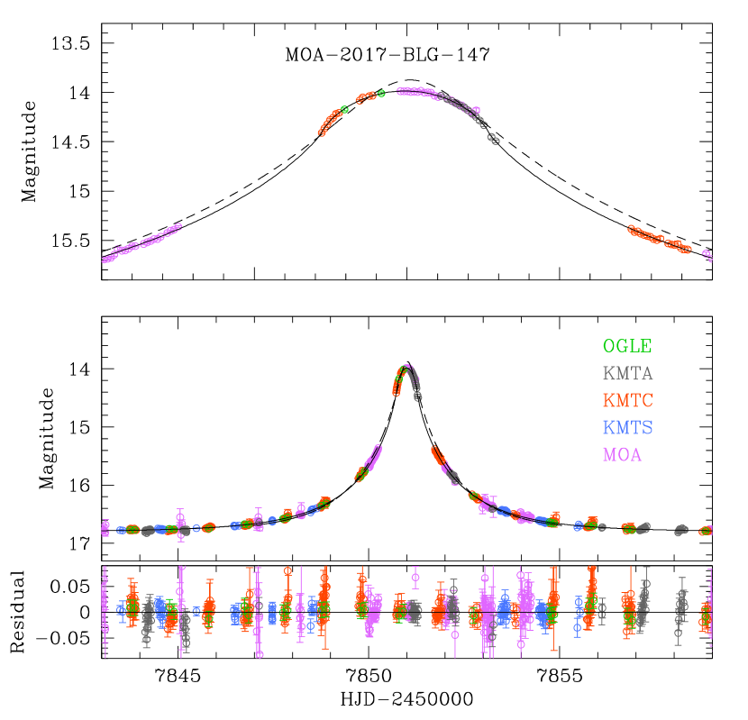
Figure 1.— Lightcurve of MOA-2017-BLG-147. The middle panel shows the whole range of lensing magnification and the top panel shows the zoom of the peak region. The solid and dashed curves superposed on the data points represent the model curves obtained with and without considering finite-source effects, respectively. The colors of the data points are set to match those of the telescopes in the legend used for the data acquisition. The bottom panel shows the residual from the model considering finite-source effects.

3. Observations and Data

The analyzed lensing events share a common observational property that the lightcurves of the events are densely observed by the major lensing surveys despite of their short timescales. All of the events are detected toward the Galactic bulge field. In Table 1, we list the positions of the events, both in equatorial coordinates (R.A., decl.)_J2000 and the corresponding galactic coordinates $(l,b)$. Also listed are the surveys that observed the events. For each event, different names are given by the individual surveys, and we list all the names according to the chronological order of the event discovery. Hereafter, we use the names given by the first discovery survey as the representative names of the events.

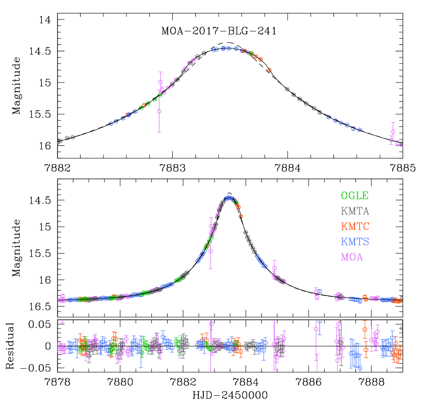
Figure 2.— Lightcurve of MOA-2017-BLG-241. Notations are same as those in Fig. 1.

The survey observations were conducted using multiple telescopes that were equipped with wide-field cameras and globally distributed in the southern hemisphere. The telescope used for the OGLE survey is located at the Las Campanas Observatory in Chile. The telescope has a 1.3 m aperture, and it is equipped with a mosaic camera that consists of 32 chips with each chip composed of $2{\rm k}\times 4{\rm k}$ pixels. The camera covers a $1.4~{}{\rm deg}^{2}$ field of view with a single exposure. The MOA 1.8 m telescope, located at the Mt. John Observatory in New Zealand, is equipped with a camera that consists of ten $2{\rm k}\times 2{\rm k}$ chips with a total $2.2~{}{\rm deg}^{2}$ field of view. The KMTNet observations were carried out using three identical 1.6 m telescopes located at the Siding Spring Observatory in Australia (KMTA), Cerro Tololo Interamerican Observatory in Chile (KMTC), and the South African Astronomical Observatory in South Africa (KMTS). The camera mounted on each of the KMTNet telescopes consists of four $9{\rm k}\times 9{\rm k}$ chips with a total $4~{}{\rm deg}^{2}$ field of view. The wide field of view of the surveys using the globally distributed telescopes enable dense and continuous coverage of the events despite their short durations. Observations by the OGLE and KMTNet surveys were conducted mostly in $I$ band with occasional observations in $V$ band. MOA observations were carried out in a customized broad $R/I$ filter.

Reduction of the data sets is conducted using the photometry codes developed by the individual survey groups based on the difference imaging method (Alard & Lupton, 1998): Woźniak (2000) (OGLE), Bond et al. (2001) (MOA), and Albrow et al. (2009) (KMTNet). For a subset of the KMTC data set, additional photometry is conducted using the pyDIA code (Albrow, 2017) for the source color measurement. We readjust the error bars of the individual data sets following the method described in Yee et al. (2012).

In Figures 1 through 3, we present the lightcurves of the MOA-2017-BLG-147, MOA-2017-BLG-241, and MOA-2019-BLG-256, respectively. As mentioned, the lightcurves of all events are affected by severe finite-source effects, and the peak regions show strong deviations from the point-source lightcurves (dashed curves). To better show the lightcurve deviation affected by finite-source effects, we present the zoom of the peak region in the upper panel of each figure. At first glance, the lightcurve of MOA-2019-BLG-256 appears to be similar to those of the other events produced by finite-source 1L1S events, but a close look shows asymmetry with respect to the peak. As we will show in the following section, the event is produced by a binary lens.

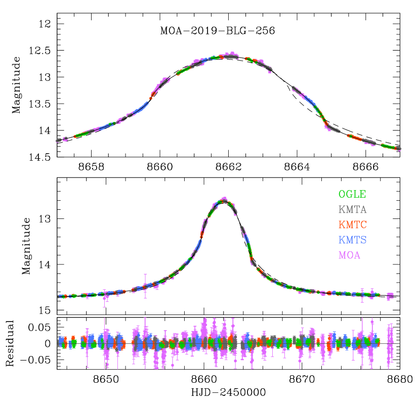
Figure 3.— Lightcurve of MOA-2019-BLG-256. The solid and dashed curves represent the model curves based on 2L1S and 1L1S modeling, respectively. For both models, finite-source effects are considered.

Table 2Best-fit lensing parameters

Parameter	MOA-2017-BLG-147	MOA-2017-BLG-241	MOA-2019-BLG-256
$t_{0}$ (${\rm HJD}^{\prime}$)	7850.994 $\pm$ 0.001	7883.473 $\pm$ 0.001	8662.089 $\pm$ 0.001
$u_{0}$	0.092 $\pm$ 0.001	0.211 $\pm$ 0.005	0.076 $\pm$ 0.001
$t_{\rm E}$ (days)	2.679 $\pm$ 0.023	1.868 $\pm$ 0.023	8.723 $\pm$ 0.008
$t_{\rm E,1}$ (days)	-	-	6.439 $\pm$ 0.006
$t_{\rm E,2}$ (days)	-	-	5.884 $\pm$ 0.005
$s$	-	-	1.968 $\pm$ 0.002
$q$	-	-	0.835 $\pm$ 0.003
$\alpha$ (rad)	-	-	2.313 $\pm$ 0.001
$\rho$	0.137 $\pm$ 0.001	0.290 $\pm$ 0.005	0.213 $\pm$ 0.001
$f_{\rm s,OGLE}$	3.076	4.345	21.310
$f_{\rm b,OGLE}$	-0.062	0.010	-1.296

Note. — ${\rm HJD}^{\prime}={\rm HJD-2450000}$. For the 2L1S event MOA-2019-BLG-256, $t_{\rm E}$ is the event timescale corresponding to the total mass of the binary lens, and $t_{\rm E,1}$ and $t_{\rm E,2}$ represent the timescales corresponding to the masses of individual lens components.

4. Modeling lightcurves

The first step for the analyses of the events is conducting modeling on the observed lightcurves. Lightcurve modeling is carried out by searching for a set of the lensing parameters that best describes the observed lightcurves. For a 1L1S event with a point source, the lensing lightcurve is described by three parameters of $t_{0}$, $u_{0}$, and $t_{\rm E}$ (Paczyński, 1986). The first two of these parameters represent the time of the closest lens-source approach and the lens-source separation (normalized to $\theta_{\rm E}$) at that time, i.e., impact parameter, respectively. For a 1L1S event in which the source radius is greater than the impact parameter, i.e., $\rho>u_{0}$, the lensing lightcurve is affected by finite-source effects. For the description of such events, one needs an additional lensing parameter of $\rho$. For 2L1S events, one needs additional parameters to describe the binary nature of the lens. These additional parameters include $s$, $q$, and $\alpha$. The parameter $s$ denotes the projected separation (normalized to $\theta_{\rm E}$), $q$ represents the mass ratio between the binary lens components, and $\alpha$ represents the incidence angle of the source trajectory with respect to the binary axis.

Lensing magnifications affected by finite-source effects differ from those of a point source. For 1L1S events, we compute finite-source magnifications using the semianalytic expressions first derived by Gould (1994a) and Witt & Mao (1994) and later refined by Yoo et al. (2004). These approximation may not be valid in the region of a very large $\rho$, and thus we check the validity of the expressions by comparing magnifications computed by using a contouring method. We find that the semianalytic expressions are valid in the cases of the analyzed events. For 2L1S events, we compute magnifications using the numerical ray-shooting method described in Dong et al. (2006). In computing finite-source magnifications, we consider the variation of the source surface brightness caused by limb darkening. To account for the limb-darkening variation, we model the surface brightness of the source star as

$$S_{\lambda}=\bar{S}_{\lambda}\left[1-\Gamma_{\lambda}\left(1-{3\over 2}\cos\theta\right)\right].$$ (3)

Here $\bar{S}_{\lambda}$ denotes the mean surface brightness, $\Gamma_{\lambda}$ is the linear limb-darkening coefficient, and $\theta$ represents the angle between the line of sight toward the source center and the normal to the source surface. The limb-darkening coefficients are estimated based on the stellar types of the source stars. As we will show in the following section, the source stars of the analyzed events are giant stars of a similar spectral type ranging from K0 to K3. Based on the stellar type, we set the limb-darkening coefficients as $\Gamma_{I}=0.41$, and $\Gamma_{\rm MOA}\sim(\Gamma_{I}+\Gamma_{R})/2=0.52$ by adopting the values from Claret (2000) under the assumption that $v_{\rm turb}=2~{}{\rm km}~{}{\rm s}^{-1}$, $\log(g/g_{\odot})=-2.4$, and $T_{\rm eff}=4500~{}K$.

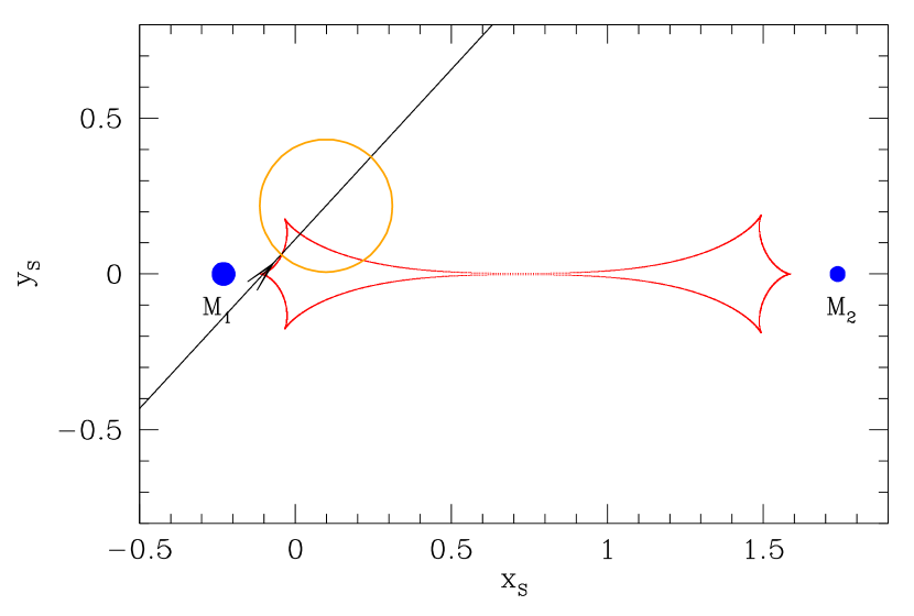
Figure 4.— Lens system configuration of the 2L1S event MOA-2019-BLG-256. The two blue dots, marked by $M_{1}$ and $M_{2}$, represent the positions of the lens components and the cuspy closed figure is the caustic. The line with an arrow is the source trajectory and the orange circle on the trajectory represents the relative size of the source. All lengths are scaled to the angular Einstein radius corresponding to the total mass of the binary lens.

We search for the best-fit lensing parameters using the combination of downhill and grid-search approaches. For events produced by single lenses, i.e., MOA-2017-BLG-147, and MOA-2017-BLG-241, lensing parameters are searched for using the downhill approach based on the Markov Chain Monte Carlo (MCMC) method. In this search, the initial values of the parameters are given considering the time of the peak, $t_{0}$, peak magnification, $A_{\rm peak}$, duration of the event, and duration of finite-source anomaly, $\Delta t$. For 1L1S events affected by severe finite-source effects, the peak magnification is approximated as $A_{\rm peak}\sim(1+4/\rho^{2})^{1/2}$ (Maeder, 1973; Riffeser et al., 2006; Agol, 2003; Han, 2016). For the 2L1S event, i.e., MOA-2019-BLG-256, the analysis is done in two steps. In the first step, we conduct grid search for the binary lensing parameters $s$ and $q$, while the other parameters are searched for using the MCMC downhill approach. In the second step, we refine the solution(s) found from the initial grid search by allowing all parameters including $s$ and $q$ to vary. Modeling 2L1S events often results in multiple solutions caused by various types of degeneracy. For MOA-2019-BLG-256, we find a unique solution without any degeneracy. We also check the possible degeneracy between binary-lens (2L1S) and binary-source (1L2S) solutions. We find that the 1L2S interpretation does not explain the observed anomaly.

In Table 2, we list the best-fit lensing parameters of the individual events. For the 2L1S event MOA-2019-BLG-256, we present three event timescales of ($t_{\rm E}$, $t_{\rm E,1}$, $t_{\rm E,2}$), in which $t_{\rm E}$ is the timescale corresponding to the total mass of the binary lens, while $t_{\rm E,1}$ and $t_{\rm E,2}$ represent the timescales corresponding to the masses of individual lens components, i.e., $t_{\rm E,1}=\sqrt{1/(1+q)}t_{\rm E}$ and $t_{\rm E,2}=\sqrt{q/(1+q)}t_{\rm E}$. The uncertainties of the parameters are estimated as the standard deviation of the points in the MCMC chain. It is found that the estimated event timescales are very short, ranging from $t_{\rm E}\sim 1.9$ days to $\sim 6.4$ days according to the timescales corresponding to the individual lens components. It is also found that the normalized source radii are very big, ranging from $\rho\sim 0.14$ to $\sim 0.29$. Also listed in the table are the flux values of the source, $f_{\rm s,OGLE}$, and blend, $f_{\rm b,OGLE}$, estimated according to the OGLE scale, in which $f=1$ for an $I=18.0$ mag star. The dominance of the source flux over the blend flux indicates that blending is negligible for all events.

Table 3Best-fit lensing parameters

Parameter	MOA-2017-BLG-147	MOA-2017-BLG-241	MOA-2019-BLG-256
$V-I$	$2.93\pm 0.07$	$2.84\pm 0.03$	$2.48\pm 0.01$
$I$	$16.59\pm 0.01$	$16.72\pm 0.01$	$15.32\pm 0.01$
$(V-I,I)_{\rm RGC}$	$(3.00,17.03)$	$(2.61,17.15)$	$(2.30,16.67)$
$(V-I,I)_{\rm RGC,0}$	$(1.06,14.51)$	$(1.06,14.65)$	$(1.06,14.30)$
$(V-I)_{0}$	$0.99\pm 0.07$	$1.30\pm 0.03$	$1.25\pm 0.01$
$I_{0}$	$14.03\pm 0.01$	$14.22\pm 0.01$	$12.95\pm 0.10$
$\theta_{*}$ ($\mu$as)	$6.94\pm 0.69$	$8.06\pm 0.60$	$14.07\pm 0.99$
$\theta_{\rm E}$ (mas)	$0.051\pm 0.005$	$0.028\pm 0.004$	$0.066\pm 0.005$
$\theta_{\rm E,1}$ (mas)	-	-	$0.049\pm 0.004$
$\theta_{\rm E,2}$ (mas)	-	-	$0.045\pm 0.003$
$\mu$ (mas yr-1)	$6.89\pm 0.69$	$5.42\pm 0.83$	$2.76\pm 0.19$
Spectral type	K0III	K3III	K3III

Note. — For the 2L1S event MOA-2019-BLG-256, $\theta_{\rm E}$ is the angular Einstein radius corresponding to the total mass of the binary lens, and $\theta_{\rm E,1}$ and $\theta_{\rm E,2}$ represent the Einstein radii corresponding to the masses of individual lens components.

In Figure 4, we present lens system configuration of the 2L1S event MOA-2019-BLG-256. The blue dot marked by $M_{1}$ and $M_{2}$ denote the positions of the binary lens components. The mass ratio between the lens components is $q=M_{2}/M_{1}=0.835\pm 0.003$, and they are separated in projection by $s=1.968\pm 0.002$. The cuspy curves represent the caustic. Because the separation between $M_{1}$ and $M_{2}$ is greater than $\theta_{\rm E}$, i.e., $s>1.0$, the caustic is composed of two segments, which are located close to the individual lens components. The line with an arrow represents the source trajectory. The orange circle on the source trajectory is marked to represent the source size with respect to the caustic. It is found that the size of the source is similar to that of the caustic located close to $M_{1}$. The source approaches and crosses the caustic multiple times. For general events with a source much smaller than a caustic, sharp spike features appear in the lensing lightcurve at the times of the individual caustic approaches and crossings. For MOA-2019-BLG-256, such a spike feature does not appear in the light curve due to the severe attenuation of the lensing magnification by finite-source effects.

5. Angular Einstein Radius

For the additional constraint of the lens mass, we estimate the angular Einstein radii of the events. The angular Einstein radius is estimated from the combination of the normalized source radius $\rho$ and the angular source radius $\theta_{*}$ by $\theta_{\rm E}=\theta_{*}/\rho$. The value of $\rho$ is measured from modeling the parts of the lightcurve affected by finite-source effects. The angular source radius is estimated from the de-reddened color $(V-I)_{0}$ and brightness $I_{0}$ of the source star using the method of Yoo et al. (2004). Following this method, we first measure the instrumental color $V-I$ and magnitude $I$ of the source and place the source location on the instrumental color-magnitude diagram (CMD). We then measure the offsets in color, $\Delta(V-I)$, and magnitude, $\Delta I$, from the centroid of red giant clump (RGC) with a location on the CMD of $(V-I,I)_{\rm RGC}$. We then estimate the calibrated de-reddened source color and magnitude, $(V-I,I)_{0}$, using the known de-reddened values of the RGC centroid by

$$(V-I,I)_{0}=(V-I,I)_{\rm RGC,0}+\Delta(V-I,I).$$ (4)

Here $(V-I,I)_{\rm RGC,0}$ represent the de-reddened color and magnitude of the RGC centroid (Bensby et al., 2013; Nataf et al., 2013).

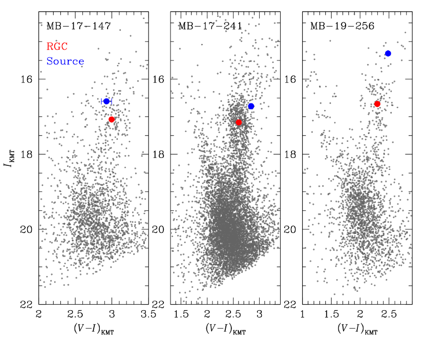
Figure 5.— Source locations (blue dots) with respect to the centroids of red giant clump (RGC, red dots) in the instrumental color-magnitude diagrams constructed based on the pyDIA photometry of the KMTC data set.

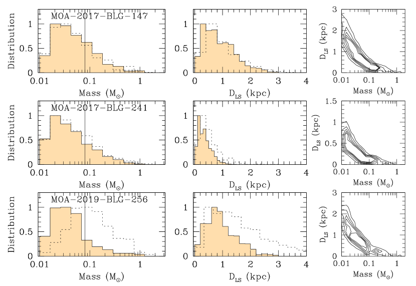
Figure 6.— Probability distributions of the lens mass ($M$) and the lens-source separation ($D_{\rm LS}$) obtained from Bayesian analyses. In each panel, the solid curve is the probability distribution obtained with the combined $t_{\rm E}+\theta_{\rm E}$ constraint, whereas the dotted curve is obtained using the constraint of only $t_{\rm E}$. The vertical line in each left panel indicates the boundary between stars and BDs, i.e., $0.08~{}M_{\odot}$. For the 2L1S event MOA-2019-BLG-256, the mass distribution is for the heavier lens component, $M_{1}$.

In Figure 5, we mark the positions of the source stars of the individual events with respect to the RGC centroids on the instrumental CMDs. The CMDs are constructed based on the pyDIA photometry of the KMTC data. In Table 3, we list the colors and magnitudes of the source, $(V-I,I)$, and the RGC centroid, $(V-I,I)_{\rm RGC}$, on the instrumental CMD. Also listed are the de-reddened colors and magnitudes of the RGC centroid, $(V-I,I)_{\rm RGC,0}$, toward the fields of the individual events (Nataf et al., 2013). We note that $I_{\rm RGC,0}$ slightly varies because the distance to the RGC centroid varies depending on the galactic longitude $l$ due to the tilt of the triaxial bulge with respect to the line of sight. With $(V-I,I)_{\rm RGC,0}$ together with the measured offsets $\Delta(V-I,I)$, the de-reddened colors and magnitudes of the source stars are computed using equation (4) and listed in Table 3. The ranges of the $I$-band magnitudes, $13.0\lesssim I_{0}\lesssim 14.2$, and the color, $1.0\lesssim(V-I)_{0}\lesssim 1.3$, indicate that the source stars of the events are bulge giant stars of a similar spectral type, ranging from K0 to K3.

With the estimated de-reddened color and magnitude, we then determine the angular source radii. This is done first by converting the measured $V-I$ color into $V-K$ color using the color-color relation of Bessell & Brett (1988) and then estimating $\theta_{*}$ using the $(V-K)/\theta_{*}$ relation of Kervella et al. (2004). Once the source radius is estimated, the angular Einstein radius is determined by $\theta_{\rm E}=\theta_{*}/\rho$.

In Table 3, we list the estimated values of $\theta_{*}$ and $\theta_{\rm E}$ for the individual events. For the 2L1S event MOA-2019-BLG-256, we additionally present the Einstein radii corresponding to the masses of the individual lens components, $\theta_{\rm E,1}$, and $\theta_{\rm E,2}$, similar to the presentation of $t_{\rm E,1}$ and $t_{\rm E,2}$ in Table 2. Also listed are the relative lens-source proper motions estimated by

$$\mu={\theta_{\rm E}\over t_{\rm E}}.$$ (5)

It is found that the angular Einstein radii are in the range of $0.028~{}{\rm mas}\lesssim\theta_{\rm E}\lesssim 0.051~{}{\rm mas}$. These values are more than an order smaller than $\sim 0.5$ mas of typical lensing events produced by low-mass lenses located roughly halfway between the observer and source. The estimated relative lens-source proper motions are in the range of $2.8~{}{\rm mas}~{}{\rm yr}^{-1}\lesssim\mu\lesssim 6.9~{}{\rm mas}~{}{\rm yr}^{-1}$. These values are smaller or similar to $\sim 5~{}{\rm mas}~{}{\rm yr}^{-1}$ of typical lensing events. This indicates that the very short timescales of the analyzed events are not caused by unusually high relative lens-source proper motions, but more likely to be caused by the low masses of the lenses.

6. Nature of Lenses

For the characterization of the lenses, we estimate the physical lens parameters of the lens mass $M$ and distance $D_{\rm L}$. In order to uniquely determine $M$ and $D_{\rm L}$, it is required to determine both the angular Einstein radius $\theta_{\rm E}$ and the microlens parallax $\pi_{\rm E}$, which are related to the lens mass and distance by

$$M={\theta_{\rm E}\over\kappa\pi_{\rm E}};\qquad D_{\rm L}={{\rm au}\over\pi_{\rm E}\theta_{\rm E}+\pi_{\rm S}},$$ (6)

where $\pi_{\rm S}={\rm au}/D_{\rm S}$ is the parallax of the source. For all the analyzed events, the angular Einstein radii are securely measured from the detections of finite-source effects. The microlens parallax is measurable by detecting deformations in lensing lightcurves caused by the deviation of the source motion from rectilinear due to the change of the observer’s position induced by the orbital motion of Earth around the sun (Gould, 1992), e.g., OGLE-2016-BLG-0156 (Jung et al., 2019). For none of the events, the microlens parallax can be measured through this annual microlens-parallax channel because the timescales of the events are too short to yield measurable deviations in the lensing lightcurves. Besides this channel, the microlens parallax can be measured from simultaneous observations of lensing events using ground-based telescopes and a space-based satellite: “space-based microlens parallax” (Refsdal, 1966; Gould, 1994b), e.g., OGLE-2015-BLG-0966 (Street et al., 2016). See more detailed discussion about the space-based microlens-parallax measurements in section 7. Unfortunately, space-based observation has been conducted for none of the events. We, therefore, estimate the physical lens parameters by conducting Bayesian analysis of the events with the constraints of the measured event timescales together with the angular Einstein radii.

Table 4Source proper motion

Event	$\mu_{\rm R.A.}$ (mas yr-1)	$\mu_{\rm decl.}$ (mas yr-1)
MOA-2017-BLG-147	$-5.348\pm 0.335$	$-7.694\pm 0.272$
MOA-2017-BLG-241	$-3.775\pm 0.450$	$-4.049\pm 0.396$
MOA-2019-BLG-256	$-2.299\pm 0.170$	$-6.973\pm 0.134$

Note. — $\mu_{\rm R.A.}$ and $\mu_{\rm decl.}$ denote the proper motions in right ascension and declination directions, respectively.

Bayesian analyses are conducted based on the prior models of the physical and dynamical distributions of astronomical objects in the Galaxy and their mass function. For the physical distributions, we use the model described in sections 2.1 and 2.2 of Han & Gould (2003). For the model of the relative lens-source motion, we adopt the non-rotating barred bulge model described in table 1 of Han & Gould (1995). For the mass function of lenses, we use the Chabrier (2003) model for stars and BDs and the Gould (2000) model for stellar remnants, i.e., black holes, neutron stars, and white dwarfs. With these models, we conduct Monte Carlo simulation to produce numerous ($4\times 10^{7}$) artificial lensing events, from which the probability distributions of the lens mass and distance are obtained. We obtain two sets of probability distributions, in which one set of distributions are obtained with only the constraint of $t_{\rm E}$, whereas the other set of distributions are obtained with the combined $t_{\rm E}$ and $\theta_{\rm E}$ constraint. We note that the source stars of all the events are bright and their proper motions are measured by Gaia (Gaia et al., 2018). In Table 4, we list the proper motions of the individual events. We consider the measured proper motions of the source stars in the Bayesian analysis.

In Figure 6, we present the probability distributions of the physical lensing parameters obtained from the Bayesian analysis. For each event, the left and middle panels show the distributions of the lens mass and the lens-source separation ($D_{\rm LS}$), respectively, and the right panel show the contours of the probability on the $M$–$D_{\rm LS}$ plane. The contours are drawn at the levels of 0.1, 0.2, 0.3, 0.4, and 0.5 with respect to the maximum probability. We note that the lenses are located very close to the source in all cases of the events and thus we present the distribution of $D_{\rm LS}$ instead of $D_{\rm L}$. The solid and dotted curves represent the distributions obtained with $t_{\rm E}+\theta_{\rm E}$ and $t_{\rm E}$ constraints, respectively. In Table 5, we list the estimated physical lens parameters. For the 2L1S event MOA-2019-BLG-256, we list the masses of both lens components, i.e., $M_{1}$ and $M_{2}$. The presented value of each parameter is estimated as the median of the probability distribution and the lower and upper uncertainties are estimated as the 16% and 84% of the distribution, respectively.

Table 5Physical lens parameters

Event	$M_{1}$ ($M_{\odot}$)	$M_{2}$ ($M_{\odot}$)	$D_{\rm LS}$ (kpc)
MOA-2017-BLG-147	$0.051^{+0.100}_{-0.027}$	-	$0.87^{+0.67}_{-0.45}$
MOA-2017-BLG-241	$0.044^{+0.090}_{-0.023}$	-	$0.36^{+0.28}_{-0.18}$
MOA-2019-BLG-256	$0.046^{+0.067}_{-0.023}$	$0.038^{+0.056}_{-0.019}$	$0.94^{+0.62}_{-0.46}$

Note. — For the 2L1S event MOA-2019-BLG-256, $M_{1}$ and $M_{2}$ denote the masses of the individual lens components.

We find that the lenses of all events share similar properties that they are very likely to be substellar objects located very close to the source stars. From the Bayesian analysis, it is estimated that the masses of the lenses are $0.051^{+0.100}_{-0.027}~{}M_{\odot}$, $0.044^{+0.090}_{-0.023}~{}M_{\odot}$, and $0.046^{+0.067}_{-0.023}~{}M_{\odot}/0.038^{+0.056}_{-0.019}~{}M_{\odot}$ for MOA-2017-BLG-147L, MOA-2017-BLG-241L, and MOA-2019-BLG-256LAB, respectively. The probability for the lens mass smaller than the lower limit for the mass of a star is about 80% for all events. The lenses of the individual events are located at the locations with the distances from the source of $D_{\rm LS}=0.87^{+0.67}_{-0.45}$ kpc, $0.36^{+0.28}_{-0.18}$ kpc, and $0.94^{+0.62}_{-0.46}$ kpc. The estimated lens masses and locations indicate that the lenses of the events are bulge BDs located close to the source stars. We note that MOA-2019-BLG-256LAB is the fourth microlensing BD binary followed by OGLE-2009-BLG-151L, OGLE-2011-BLG- 0420L (Choi et al., 2013), and OGLE-2016-BLG-1469L (Han et al., 2017).

It is found that the additional constraint provided by the angular Einstein radius helps to reveal the substellar nature of the lenses. For MOA-2017-BLG-147 and MOA-2017-BLG-241, the probability distributions of $M$ and $D_{\rm LS}$ with the additional constraint of $\theta_{\rm E}$ are not much different from the distributions obtained with only $t_{\rm E}$ constraint, indicating that the additional constraint of $\theta_{\rm E}$ is not very strong. However, for MOA-2019-BLG-256, the additional constraint of $\theta_{\rm E}$ substantially shifts the most probable lens mass and location toward lower masses and closer to the source, respectively. For the former two events, the event timescales, $t_{\rm E}<2.7$ days, are very short and thus the timescale alone constrains that the lens is likely to be a substellar object. On the other hand, the event timescales of MOA-2019-BLG-256, $t_{\rm E}\sim 8.7$ days, is relatively long and the BD nature of the lens can be constrained with the additional constraint of the very small $\theta_{\rm E}$. The very small $\theta_{\rm E}$ values also tightly constraint the lens locations, i.e., very close to the source, because $\theta_{\rm E}\propto(D_{\rm LS}/D_{\rm L}D_{\rm S})^{1/2}$.

7. Discussion

Although the probability of the lenses to be BDs is high, the ranges of the lens masses estimated from the Bayesian analysis are rather big. To firmly identify the BD nature of the lenses, it is desirable to uniquely determine the lens masses by additionally measuring the values of the microlens parallax.

We point out that the microlens parallax values and thus the lens masses of the events could have been uniquely determined if the events had been observed using a satellite separated from Earth by a substantial fraction of an au. Space-based microlens-parallax measurement is optimized when the projected Earth-satellite separation as seen from the lens-source line of sight (projected satellite separation), $D_{\perp}$, comprises an important portion of the physical Einstein radius projected onto the plane of the observer (projected Einstein radius), $\tilde{r}_{\rm E}=(D_{\rm S}/D_{\rm LS})r_{\rm E}$. Here $r_{\rm E}=D_{\rm L}\theta_{\rm E}$ represents the physical Einstein radius. If $D_{\perp}\gg\tilde{r}_{\rm E}$, the lensing magnifications observed by ground-based telescopes would be difficult to be observed by a space-based satellite because the impact parameter of the lens-source approach seen from the satellite would be too big to induce lensing magnifications. If $D_{\perp}\ll\tilde{r}_{\rm E}$, in contrast, the difference between the two lensing lightcurves obtained from the ground- and space-based observations would be too small to securely measure $\pi_{\rm E}$.

Considering the Spitzer telescope as an example of a satellite in a heliocentric orbit, we estimate the values of $r_{\rm E}$, $\tilde{r}_{\rm E}$, and $D_{\perp}$ and list them in Table 6. We note that the projected Einstein radius $\tilde{r}_{\rm E}$ is much bigger than $r_{\rm E}$ because $\tilde{r}_{\rm E}$ is inversely proportional to the lens-source distance, i.e., $\tilde{r}_{\rm E}=(D_{\rm S}/D_{\rm LS})r_{\rm E}$, and the lens-source separations are very small for the analyzed events. We also list the ratios of $D_{\perp}/\tilde{r}_{\rm E}$ corresponding to the Spitzer telescope locations at the times of the events. The ratios are in the range of $0.3\lesssim D_{\perp}/\tilde{r}_{\rm E}\lesssim 0.6$, which are optimal ratios for secure $\pi_{\rm E}$ measurements.

Table 6Projected Einstein radius

Event	$r_{\rm E}$ (au)	$\tilde{r}_{\rm E}$ (au)	$D_{\perp}$ (au)	$\tilde{r}_{\rm E}/D_{\perp}$ (au)
MOA-2017-BLG-147	0.36	3.3	1.59	0.48
MOA-2017-BLG-241	0.21	4.8	1.59	0.33
MOA-2019-BLG-256	0.35	2.9	1.73	0.60

Note. — $\tilde{r}_{\rm E}$ denotes the physical Einstein radius projected onto the plane of the observer and $D_{\perp}$ represents the projected Earth-Spitzer separation as seen from the lens-source line of sight.

For none of the events, Spitzer observation could be conducted because of the combined reasons that the current Spitzer microlensing campaign (Calchi Novati et al., 2015) has been conducted in a follow-up mode together with the fact that the timescales of the events are very short. According to the protocol of the Spitzer sample selection (Yee et al., 2015), very short-timescale events are unlikely to be selected because immediate follow-up observation is difficult due to the relatively long period (a week) of uploading observation sequences and the time required to prepare the sequences. These difficulties of observing short-timescale events can be overcome if space-based observations are carried in a survey mode simultaneously with a ground-based survey. Another important reason for difficulty of observing the events is the short time window, $\sim 40$ days, through which the bulge field is observable simultaneously from Spitzer and from the ground. The Spitzer window ran during 7927–7969 and 8671–8712 in the 2017 and 2019 seasons, respectively. As a result, all of the events were at (or nearly at) baseline by the time Spitzer observations started.

8. Summary and conclusion

We investigated strong candidate BD-lens events found from the search for lensing events not only with short timescales but also with very small angular Einstein radii. By imposing the criteria of $t_{\rm E}\lesssim 6~{}{\rm days}$ and $\theta_{\rm E}\lesssim 0.05~{}{\rm mas}$ for events detected since the 2016 season, we found three events including MOA-2017-BLG-147, MOA-2017-BLG-241, and MOA-2019-BLG-256, in which the lens of the last event is a binary. By measuring the event timescales and angular Einstein radii from lightcurve modeling followed by Bayesian analyses of the events with the combined constraint of $t_{\rm E}$ and $\theta_{\rm E}$, we estimated that the lens masses of the individual events were $0.051^{+0.100}_{-0.027}~{}M_{\odot}$, $0.044^{+0.090}_{-0.023}~{}M_{\odot}$, and $0.046^{+0.067}_{-0.023}~{}M_{\odot}/0.038^{+0.056}_{-0.019}~{}M_{\odot}$. We pointed out that uniquely determining lens masses of short timescale events by additionally measuring microlens-parallax values required survey-mode space-based observation using a satellite in a heliocentric orbit.

References

- Agol (2003) Agol, E. 2003, ApJ, 594, 449
- Alard & Lupton (1998) Alard, C., & Lupton, R. H. 1998, ApJ, 503, 325
- Albrow (2017) Albrow, M. 2017, MichaelDAlbrow/pyDIA: Initial Release on Github, doi: 10.5281/zenodo.268049
- Albrow et al. (2009) Albrow, M., Horne, K., Bramich, D. M., et al. 2009, MNRAS, 397, 2099
- Bensby et al. (2013) Bensby, T., Yee, J. C., Feltzing, S., et al. 2013, A&A, 549, 147
- Bessell & Brett (1988) Bessell, M. S., & Brett, J. M. 1988, PASP, 100, 1134
- Bond et al. (2001) Bond, I. A., Abe, F., Dodd, R. J., et al. 2001, MNRAS, 327, 868
- Calchi Novati et al. (2015) Calchi Novati, S., Gould, A., Udalski, A., et al. 2015, ApJ, 804, 20
- Chabrier (2003) Chabrier, G. 2003, ApJ, 586, L133
- Choi et al. (2013) Choi, J.-Y., Han, C., Udalski, A., et al. 2013, ApJ, 768, 129
- Choi et al (2012) Choi, J.-Y., Shin, I.-G., Park, S. -Y., et al, 2012, ApJ, 751, 41
- Claret (2000) Claret, A. 2000, A&A, 363, 1081
- Dong et al. (2006) Dong, S., DePoy, D. L., Gaudi, B. S., et al. 2006, ApJ, 642, 842
- Gaia et al. (2018) Gaia Collaboration, Brown, A. G. A., Vallenari, A., et al. 2018, A&A, 616, A1
- Gould (1992) Gould, A. 1992, ApJ, 392, 442
- Gould (1994a) Gould, A. 1994a, ApJ, 421, L71
- Gould (1994b) Gould, A. 1994b, ApJ, 421, L75
- Gould (2000) Gould, A. 2000, ApJ, 535, 928
- Han (2016) Han, C. 2016, ApJ, 820, 53
- Han & Gould (1995) Han, C., & Gould, A. 1995, ApJ, 447, 53
- Han & Gould (2003) Han, C., & Gould, A. 2003, ApJ, 592, 172
- Han et al. (2017) Han, C., Udalski, A., Sumi, T., et al. 2017, ApJ, 843, 59
- Jung et al. (2019) Jung, Y. Kil, Han, C., Bond, I. A., et al. 2019, ApJ, 872, 175J
- Kervella et al. (2004) Kervella, P., Thévenin, F., Di Folco, E., & Ségransan, D. 2004, A&A, 426, 29
- Kim et al. (2016) Kim, S.-L., Lee, C.-U., Park, B.-G., et al. 2016, JKAS, 49, 37
- Maeder (1973) Maeder, A. 1973, A&A, 26, 215
- Mróz et al. (2018) Mróz, P., Ryu, Y.-H., Skowron, J., et al. 2018, AJ, 155, 121
- Mróz et al. (2019) Mróz, P., Udalski, A., Bennett, D. P., et al. 2019, A&A, 622, A201
- Nataf et al. (2013) Nataf, D. M., Gould, A., Fouqué, P., et al. 2013, ApJ, 769, 88
- Paczyński (1986) Paczyński, B. 1986, ApJ, 304, 1
- Refsdal (1966) Refsdal, S. 1966, MNRAS, 134, 315
- Riffeser et al. (2006) Riffeser, A., Fliri, J., Seitz, S., & Bender, R. 2006, ApJS, 163, 225
- Street et al. (2016) Street, R. A., Udalski, A., Calchi Novati, S., et al. 2016, ApJ, 819, 93
- Udalski et al. (2015) Udalski, A., Szymański, M. K., & Szymański, G. 2015, Acta Astron., 65, 1
- Witt & Mao (1994) Witt, H. J., & Mao, S. 1994, ApJ, 430, 505
- Woźniak (2000) Woźniak, P. R. 2000, Acta Astron., 50, 42
- Yee et al. (2012) Yee, J. C., Shvartzvald, Y., Gal-Yam, A., et al. 2012, ApJ, 755, 102
- Yee et al. (2015) Yee, J. C., Gold, A., Beichman, C., et al. 2015, ApJ, 810, 155
- Yoo et al. (2004) Yoo, J., DePoy, D. L., Gal-Yam, A., et al. 2004, ApJ, 603, 139