More Connected, More Active:
Galaxy Clusters and Groups at $z\sim 1$ and The Connection between Their Quiescent Galaxy Fractions and Large-scale Environments

Abstract

High-redshift galaxy clusters, unlike local counterparts, show diverse star formation activities. However, it is still unclear what keeps some of the high-redshift clusters active in star formation. To address this issue, we performed a multi-object spectroscopic (MOS) observation of 226 high-redshift ($0.8<z<1.3$) galaxies in galaxy cluster candidates and the areas surrounding them. Our spectroscopic observation reveals six to eight clusters/groups at $z\sim 0.9$ and $z\sim 1.3$. The redshift measurements demonstrate the reliability of our photometric redshift measurements, which in turn gives credibility for using photometric redshift members for the analysis of large-scale structures (LSSs). Our investigation of the large-scale environment ($\sim$10 Mpc) surrounding each galaxy cluster reveals LSSs — structures up to $\sim 10$ Mpc scale — around many of, but not all, the confirmed overdensities and the cluster candidates. We investigate the correlation between quiescent galaxy fraction of galaxy overdensties and their surrounding LSSs, with a larger sample of $\sim 20$ overdensities including photometrically selected overdensities at $0.6<z<0.9$. Interestingly, galaxy overdensities embedded within these extended LSSs show a lower fraction of quiescent galaxies ($\sim 20\%$) than isolated ones at similar redshifts (with a quiescent galaxy fraction of $\sim 50\%$). Furthermore, we find a possible indication that clusters/groups with a high quiescent galaxy fraction are more centrally concentrated. Based on these results, we suggest that LSSs are the main reservoirs of gas and star-forming galaxies to keep galaxy clusters fresh and extended in size at $z\sim 1$.

1 Introduction

In the local universe, galaxies show distinct properties in different environments, such as morphology (e.g., Bamford et al., 2009; Ko et al., 2012), color, star-formation rate (SFR), and size (e.g., Cooper et al., 2012; Papovich et al., 2012; Strazzullo et al., 2013; Yoon et al., 2017). Especially, star-formation (SF) activities are clearly distinguished depending on their environment (e.g., Lewis et al., 2002; Kauffmann et al., 2004; Blanton et al., 2005; Bamford et al., 2009), in the sense that galaxies in field are on average bluer or more actively forming stars than those in clusters.

This picture of environmental dependence of galaxy properties becomes more complicated at higher redshifts. The SF activities in galaxy clusters are found to be evolving fast from $z=0$ to 1 with a higher SF rate (SFR) at higher redshifts (Saintonge et al., 2008; Bai et al., 2009; Tran et al., 2010; Webb et al., 2013), and the evolution seems faster in clusters than in the field (Alberts et al., 2014). Consequently, the environmental dependence becomes weaker or even reversed with increasing redshifts (e.g., Butcher & Oemler, 1984; Elbaz et al., 2007; Cooper et al., 2008; Muzzin et al., 2012; Scoville et al., 2013), although on average, the environmental dependence persists out to $z\sim 1$ (Patel et al., 2009; Quadri et al., 2012; van der Burg et al., 2013; Jian et al., 2018).

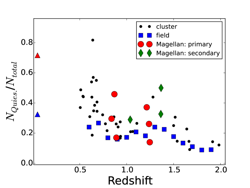
Figure 1: The fraction of quiescent galaxies in clusters (small black circles) and field (blue squares). The main target clusters of our Magellan observation are shown as large red circles, and green diamonds show secondary Magellan targets. The quiescent galaxy fraction is defined as the fraction of galaxies whose sSFR (SFR/M_∗) values are smaller than 1/($3\times t(z)$) yr^-1 and whose stellar masses are greater than $10^{9.1}$ M_⊙. The red and blue triangles are the corresponding local values for the cluster and field, respectively from Baldry et al. (2006).

The weakened environmental dependence is due to dense environments having a variety of SF activities. Recently, Lee et al. (2015, hereafter, L15) analyzed the evolution in the fraction of quiescent galaxies in clusters and in field at $0.5<z<2$ using the multi-wavelength data of the Ultra Deep Survey (UDS; Almaini et al., 2007). Figure 1 shows the quiescent galaxy fraction of individual galaxy clusters found in the UDS field as well as the mean values for field galaxies from L15. The quiescent fraction is measured for galaxies with a stellar mass greater than $10^{9.1}$ M_⊙. While local galaxy clusters have similar quiescent galaxy fractions of $\sim 0.7$ (Baldry et al., 2006), we can see a broad range in the quiescent galaxy fraction of galaxy clusters at $z>0.6$ with values ranging from 0.1 to 0.8. This cluster-by-cluster variation in the quiescent galaxy fraction persists up to redshifts as high as $z\sim 1.6$, at which point the difference between clusters and the field starts to disappear (see also, Hayashi et al., 2011; Brodwin et al., 2013; Alberts et al., 2016; Cooke et al., 2016). Hayashi et al. (2019), using the data from Hyper Suprime-Cam (HSC) Subaru Strategic Program (SSP) survey (Aihara et al., 2018), also found that there is a variation in the quiescent galaxy fraction among $z\sim 0.9$ clusters which are embedded in the large-scale structure (LSS) of the CL1604 supercluster (Lemaux et al., 2012). The evolution in the quiescent fraction, especially out to $z\sim 1$, is closely related to the SF quenching mechanism (e.g., L15; Peng et al., 2010), and close investigation of these high redshift clusters can possibly offer insight on what controls SF activities in dense environments. At $z>1$, more clusters are being identified with strong SF activity (Brodwin et al., 2013; Alberts et al., 2014, 2016; Shimakawa et al., 2018). The insight gathered from $z\sim 1$ clusters can help understand the underlying mechanism for the SF activity in clusters at $z>1$.

The large-scale environment of clusters, which is well beyond the scale of individual galaxy clusters, can also be considered as a key factor that regulates SF in clusters. At $z\sim 0.23$, Fadda et al. (2008) found an enhancement in the fraction of SF galaxies within filamentary structures outside the Abell 1763 cluster, speculating that these filaments are feeding the cluster with the infall of galaxies and galaxy groups. This higher SF fraction may be due to cold gas retention or enhanced galaxy-galaxy interaction within these structures. Studying the cluster A3266, Bai et al. (2009) suggested that the similarity of infrared (IR) luminosity function between field and clusters may due to the continual replenishment of star-forming galaxies from the field to the cluster. Mahajan et al. (2012) also found the increase in the SF activity on the outskirts of nearby ($0.02\leq z\leq 0.15$) clusters. Interestingly, this increase in SF is more commonly seen in dynamically unrelaxed clusters, which are in the course of assembly through falling from surrounding filamentary structures. At intermediate redshifts, Geach et al. (2011) studied large-scale (15 Mpc scale) environments around $z\sim 0.55$ galaxy clusters. They showed that, outside of the cluster, there are intermediate density regions where the fraction of SF galaxies is enhanced, while the mean SFR shows no significant environmental dependence.

At higher redshifts, Lubin et al. (2009), studying the large-scale environment of two clusters at similar redshift $z\sim 0.8$, found that one of them is more isolated and has a large quiescent galaxy population, while another is in the process of four-way group-group merger with a high fraction of star forming galaxies ($\sim 80\%$). And, Koyama et al. (2008) found that the fraction of the IR bright galaxies, supposedly star-forming galaxies, is enhanced at the medium density environment of a $z=0.81$ cluster, suggesting enhanced SF activities in filaments and groups. At $z\sim 0.85$, Pintos-Castro et al. (2013) showed that the star-forming galaxy fraction is higher at intermediate density regions — the outskirts of clusters, groups, and filaments — compared to higher (cluster-core region) or lower (field) density regions. Darvish et al. (2014) also showed that the fraction of H$\alpha$ emitters is enhanced in the filamentary structures at $z\sim 0.84$. In summary, intermediate density regions, such as filaments around clusters, seem to provide an environment that is favourable to sustain SF activities, possibly via cold gas accretion/replenishment (e.g., Kleiner et al., 2017), than field or cluster environments. Connected with these filamentary, intermediate density structures, galaxy clusters can be supplied with fresh SF galaxies from these structures, which increases the fraction of SF galaxies in clusters (e.g., Ellingson et al., 2001; Ebeling et al., 2004; Tran et al., 2005; Saintonge et al., 2008; Koyama et al., 2018).

In this regard, Aragon-Calvo et al. (2019) suggested a cosmic web detachment (CWD) model as a mechanism to quench SF in clusters. According to this model, the SF activities are maintained to some extent in clusters due to the supply of cold gas and SF galaxies through the cosmic web. However, after the cosmic web is detached, galaxies in clusters lose the driver for continuing SF. This model can be tested effectively at $z\sim 1$ clusters, where we can find clusters with many distinct levels of quiescent galaxy fraction (e.g., L15).

To understand what makes the observed cluster-by-cluster variation in the SF property, we performed multi-object spectroscopy of 226 galaxies in the UDS field to study clusters/groups at $z\sim 1$ and LSSs associated with them. With the data, we study the quiescent fraction of galaxies in overdensities at $0.6<z<1.3$ and examine how the presence of surrounding LSSs influences the SF activities in clusters/groups. The quiescent galaxy fraction is a useful indicator of SF activity when there is a lack of deep, high resolution IR data, by not being affected by missing a small number of highly obscured (therefore high SFR) galaxies in the sample, nor uncertainties in deriving the exact values of SFRs in the absence of IR data.

In Section 2, we explain the data and sample and the spectroscopic observation with the Magellan telescope as well as the data reduction and redshift measurement. Based on these spectroscopic data, we show the reliability of our photometric redshift measurement and stellar population estimation from spectral energy distribution (SED)-fitting in Section 3. We present properties of spectroscopically studied galaxy clusters/groups as well as LSSs near these clusters in Sections 4 and 5, respectively. Some of these are newly discovered structures. In Section 6, we discuss the causes of variation in SF properties of individual overdensities. Then, we summarize our results in Section 7. We adopt the standard flat $\rm{\Lambda}$CDM cosmology with ($\Omega_{m},\Omega_{\Lambda}$) = (0.3, 0.7) and $H_{0}$ = 70 km s^-1 Mpc^-1, which is supported by observations in the past decades (e.g., Im et al., 1997). All magnitudes are given in the AB magnitude system (Oke, 1974).

2 Data

2.1 Sample

Our sample is drawn from high-redshift ($0.5<z<2.0$) cluster candidates that are selected from a 0.77 deg² area of the entire UDS field. Our cluster-finding algorithm is described in L15 (also in Kang & Im, 2015). Briefly, galaxy cluster candidates are selected as overdense regions, where the galaxy surface number density is higher than the field value by more than 4 $\sigma$ at each redshift bin. Photometric redshifts ($z_{phot}$s) of galaxies are estimated to the accuracy of $\Delta z$/($1+z$) = 0.028, using EAZY (Brammer et al., 2008). The redshift bins have the width of $\pm 0.028\times(1+z)$, and the step size is 0.02. Stellar masses and SFRs of galaxies are measured through SED-fitting, assuming the Chabrier (2003) IMF and delayed star-formation histories (SFHs) (e.g., Lee et al., 2010). We applied the stellar mass cut of log (M_∗/M_⊙) $\geq 9.1$. Cluster member galaxies are those within a 1 Mpc radius and within the redshift range of the mean photometric redshift uncertainty (i.e., $\pm 0.028\times(z_{cl}+1)$), where $z_{cl}$ is the cluster redshift. Refer to L15 for a more detailed explanation about the procedure of galaxy cluster selection and the estimation of stellar population property through SED-fitting. We note that, unlike the methods that rely on the existence of a well-developed red sequence, our cluster finding method is not biased against active star-forming clusters, which is crucial in this study (also see Trevese et al. (2007) and Eisenhardt et al. (2008) for other photometric redshift-based cluster finding methods). There are 46 cluster candidates, and they have halo masses of log ($M_{200}/M_{\odot}$) in the range of [13.4,14.2] (L15), where the $M_{200}$ values are obtained by converting the sum of stellar masses of the member galaxy candidates by dividing it with a factor of 0.013, where the factor of 0.013 is the mean ratio of the sum of the stellar mass to the X-ray based cluster mass of 13 clusters that are in common with L15 and the sample of Finoguenov et al. (2010, hereafter, F10).

2.2 Spectroscopy Targets

Among the 46 cluster candidates, we selected targets for the multi-object spectroscopy using the Magellan Baade 6.5 m Telescope at Las Campanas Observatory, Chile, based on (1) the SF property — covering a wide range in quiescent galaxy fraction, (2) redshift — residing at similar redshifts at $z\sim 1$, and (3) their vicinity with each other — to be within the field-of-view (FoV) of the Inamori Magellan Areal Camera and Spectrograph (IMACS; Dressler et al., 2011) instrument. Based on these criteria, we select six cluster candidates that show different quiescent galaxy fractions while residing at similar redshifts, $z\sim 0.9$ and 1.2 as our main targets. These target cluster candidates are shown as red circles in Figure 1. As can be seen in this figure, some of the target cluster candidates have a similar fraction of quiescent galaxies with field galaxies at a similar epoch, while some have significantly larger quiescent fractions. Then, three additional cluster candidates, which are at $z\sim 1.0$ and 1.4, are also selected as spectroscopic targets because these clusters are within the FoV of Magellan/IMACS ($27\arcmin$ diameter circle). These cluster candidates are shown as the green diamonds in Figure 1. In addition, field galaxies that are at similar photometric redshift ranges with the selected cluster targets and within the same Magellan FoV are also included. In summary, we observed 6 clusters at $z\sim 0.9$ and 1.2 with on average $\sim 25$ slits assigned per cluster, and 3 additional clusters at $z\sim 1.0$ and 1.4 with much less slit assignments ($\sim 13$ per cluster). The remaining slits were assigned to field galaxies and other objects of interest.

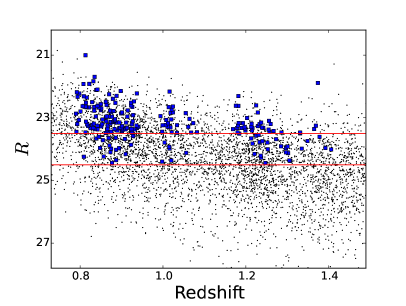
Figure 2: $R$-band magnitude versus redshift of galaxies in the Magellan/IMACS field of view (the black dots). The target galaxies for the spectroscopic observation are shown as the blue squares. The magnitude limits for the target selection, $R<23.5$ (the first priority) and $R<24.5$ (the second priority) are indicated as the red lines.

Target galaxies are selected based on their $R$-band magnitude. First, only galaxies brighter than $R\leq 24.5$ are selected. Then, among these, higher priority is assigned to galaxies that are brighter than $R\leq 23.5$ in the mask generation procedure. Figure 2 shows the photometric redshifts and $R$-band magnitudes of galaxies within the FoV of Magellan/IMACS (shown as black points) as well as the target galaxies (shown as blue squares).

In Table 1, we list our target cluster candidates, along with the number of member galaxy candidates observed and the number of the observed galaxies with spectroscopic redshift identification.

2.3 Spectroscopic Observation and Data Reduction

We prepared two separate masks for our observation of the same sky region with slightly different slit assignments. Basically, the same faint ($R\geq 23.5$) galaxies are included in both masks, while different bright galaxies are targeted in different masks. In addition, $i$-dropout candidate galaxies are included with the lowest priority for serendipitous discovery of $z\sim 6$ bright star-forming galaxies or quasars. About 250 slits are assigned for the targets above in each mask, among which $43\%$ are for the cluster galaxy candidates, $39\%$ for the field galaxies, and $17\%$ for the $i$-band dropout candidates. One slit in each mask is assigned for a standard (K-type) star.

The multi-object spectroscopic (MOS) observations were carried out using the IMACS f/2 camera on the Magellan/Baade telescope in September 2014 and in September 2015. We prepared two masks for our observation as explained in the above paragraph. The slit length and width were set at $6\arcsec\times 1\arcsec$, respectively. The total exposure time for each mask was 2.5 hours, which was divided into five 30-minute exposures. The average seeing was $0.8\arcsec$ and $1.1\arcsec$, for the 2014 and 2015 runs, respectively. We used the Grism with 200 lines per millimeter and the WB6300-9500 filter to provide a wavelength coverage of 630 to 950 nm at the spectral resolution of R$\sim 650$, which is suitable to catch major spectroscopic features of galaxies of our interest.

Data reduction was done using the Carnegie Observatories System for Multi Object Spectroscopy (COSMOS), which is a software package offered from Carnegie Observatories to reduce spectroscopic data taken with IMACS and LDSS3 instruments. For wavelength calibration, He, Ne, Ar arc frames were used. Following the standard COSMOS routine, we did flat fielding and bias subtraction from science frames. After the sky subtraction, we extracted two-dimensional (2D) spectra and stacked them onto one combined 2D spectrum. The bulk of cosmic rays were removed in the process. For the faint ($R\geq 23.5$) objects, we stacked all 10 single-exposed 2D spectra from two masks for higher S/N. More details about the data reduction are described in the COSMOS cookbook (Villanueva 2014). One dimensional (1D) spectra for each source were extracted from the combined 2D spectrum using the extraction width that corresponds to twice the average seeing value in 2014 and 2015 each. With a standard star included in the mask, we did flux calibration.

2.4 Spectroscopic Redshift

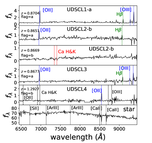
Figure 3: Examples of Magellan/IMACS spectra of cluster member galaxies as well as a star. The redshift in each panel is the measured spectroscopic redshift for each galaxy. Several emission or absorption spectral features are shown as colored vertical lines. In the fifth panel, we show the spectrum of a $z=1.293$ galaxy, based on the strong [O II] emission line at $\lambda\sim 8545$ Å. If this line was H$\beta$ (meaning the redshift of this galaxy was $z\sim 0.758$), other lines should have appeared at the wavelengths marked with black dotted lines (and labeled in black). The absence of these lines makes the redshift determination of this galaxy more reliable. In the bottom panel, we show a stellar spectrum.

From the extracted 1D spectra, we determined the redshifts of galaxies using the SpecPro software (Masters & Capak, 2011). The main spectral features for the redshift identification are [O II] 3727, H${\beta}$, H${\gamma}$, and [O III] emission lines, Ca H$\&$K and G band absorption lines, and the 4000 $\rm{\AA}$ break. We show example spectra of several confirmed cluster member galaxies in Figure 3. In each panel, we show the determined spectroscopic redshift as well as the line features used in the redshift determination.

We assigned quality flag ‘a’ for galaxies whose redshift measurements are based on two or more emission or absorption lines. If the redshift determination is based on a single line feature (we consider Ca H$\&$K lines as a single feature), the quality flag ‘b’ is given. For majority of galaxies at $z<1.2$, we can determine the redshift based on multiple spectral features as well as the clear continuum shape (quality flag ‘a’). For many $z>1.2$ galaxies, the redshift measurement was done based on a single feature, [O II] $\lambda 3727$, while we can also see the Ca H$\&$K absorption lines in some cases. However, even when only a single emission line is seen in the spectrum, our redshift determination at $z>1.2$ is reliable because (1) we do not see other significant emission features that should be seen if the given line is not [O II], and (2) the photometric redshift measured from multi-band SEDs also matches well within the photometric redshift uncertainty. For example, for a galaxy shown in the fifth panel of Figure 3, if the emission line at $\lambda\sim 8545$ Å, which is identified as [O II] (giving this galaxy a redshift of 1.293), were H${\beta}$ (i.e., at $z\sim 0.758$), [O II] and [O III] lines should have been seen at $\lambda\sim 6551$ Å, and at $\lambda\sim 8720$ and 8804 Å, as shown with the black dotted lines in this panel.

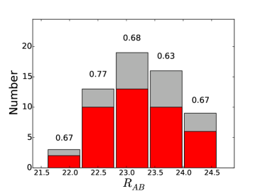
Figure 4: The $R$-band magnitude dependent number distribution of cluster member galaxy candidates. Gray bars show the number of member galaxy candidates of which redshifts are measured from our Magellan observation presented in this work. Red bars show the number of galaxies that are confirmed as the members of galaxy clusters. Numbers above gray bars are the fraction of confirmed galaxies as cluster members at each magnitude bin. As can be seen here, the $R$-band dependence is not significant.

We determined the redshifts of 173 galaxies out of 274 targets, which gives the redshift determination rate (or success rate) of $\sim 63\%$. If we exclude $i$-dropout candidates, the success rate increases to $\sim 76\%$. Figure 4 shows the cluster member confirmation rate from spectroscopic redshift as a function of $R$-band magnitude. Table 2 shows all the target galaxies of our Magellan observation, including those whose redshifts were not measured, as well as stars.

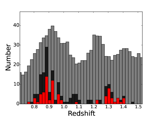
Figure 5: Distribution of spectroscopic redshifts from Magellan observation. The red histogram shows the distribution of candidate cluster galaxies while the black histogram is for total (cluster$+$field) galaxies. Both distributions show broad peaks at $z\sim 0.9$ and $z\sim 1.3$ where our six main cluster targets reside (refer to Section 2.1 for detail.). The light gray histogram shows the photometric redshift distribution of the mass-limited (log ($M_{*}/M_{\odot}$)$\geq 9.1$) UDS galaxies, whose numbers are scaled down for visual purpose.

Among 173 galaxies with secure redshifts from our observation, about $44\%$ are cluster galaxy candidates, while the remaining galaxies are field ones. Figure 5 shows the distribution of the spectroscopic redshift of all 173 galaxies in black. The red histogram is for cluster galaxy candidates. As explained in Section 2.2, field galaxy targets are selected for being at similar redshifts with cluster galaxies. Therefore, the redshift distribution of these two populations show similar trends with broad peaks at $z\sim 0.9$ and $z\sim 1.3$.

3 Accuracy of Photometric Redshift and SED-Fitting

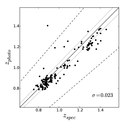
Figure 6: Comparison of spectroscopic redshifts from our Magellan observation to photometric redshifts. The photometric redshift uncertainty, is $|\Delta z|$/($1+z_{spec})=0.023$, where $|\Delta z|$ = $|z_{phot}-z_{spec}|$. Dotted and dashed lines correspond to the $|\Delta z|$/$(1+z_{spec})=0.023$ and 0.15, respectively.

Figure 6 shows the comparison of the spectroscopic redshifts obtained from our Magellan observation and the photometric redshifts from L15, which were measured using the broadband photometric data from optical to mid-IR. The normalized median absolute deviation (NMAD) between photometric and spectroscopic redshifts, $|\Delta z|$/($1+z_{spec}$), based on our Magellan observation, is 0.023, which is similar to the value reported in L15 (0.028). Here, $\Delta z$ is the difference between spectroscopic and photometric redshifts. There is only one outlier with $|\Delta z|/(1+z_{spec})$ greater than 0.15.

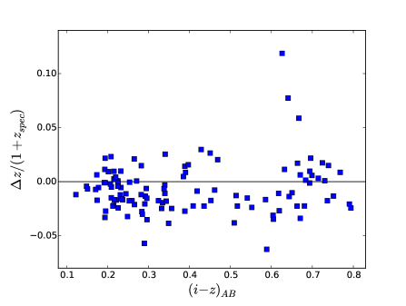
Figure 7: $(i-z)$ colour dependence of normalized photometric redshift error, $\Delta z$/($1+z_{spec}$) for $z\sim 0.9$ galaxies. There is no clear colour dependence in redshift error. We exclude one outlier ($|\Delta z|$/$(1+z_{spec})>0.15$) in this figure.

We check if there is any color dependence in photometric redshift error as a function of $(i-z)$ colour. Here, we focus on $z\sim 0.9$ galaxies, and for these galaxies, $(i-z)$ colour brackets the $4000\AA$ break, a common strong spectral feature for photometric redshift estimates. As can be seen in Figure 7, photometric redshift error does not show any clear colour dependence. The values of mean and standard deviation of normalized redshift error are $-0.008\pm 0.017$ for blue galaxies (i.e., galaxies with $(i-z)<0.5$), and $-0.003\pm 0.033$ for red ($(i-z)\geq 0.5$) galaxies. Note that we exclude one red outlier (with $\Delta z/(1+z_{spec})>0.15$ and $(i-z)>0.5$) in this calculation and in Figure 7.

For the spectroscopically identified overdensities (refer to the next section for the detailed explanation about the spectroscopic identification and properties of the clusters/groups), $31.7\%$ of the spectroscopically identified galaxy candidates turned out to be non-members — giving the member confirmation rate of $68.3\%$. The high confirmation rate suggests that a photometric redshift can trace large-scale galaxy overdensities reasonably well. This confirmation fraction does not show a clear dependence on the magnitude of galaxies as shown in Figure 4.

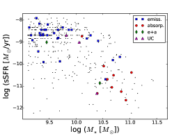
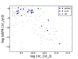
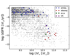
Figure 8: Stellar-mass–sSFR diagram of galaxies at $z\sim 0.9$ (Left) and $z\sim 1.2$ (Right). Panels in the upper row are for cluster candidate galaxies, and the lower row is for field galaxies. Blue squares represent galaxies with emission features only in their spectrum, while red circles are the ones with absorption features only. Green diamonds are the galaxies with both emission and absorption features, and purple triangles are the galaxies whose spectral features are weak. Black dots represent the galaxies with photometric redshifts only.

In Figure 8, we show the stellar-mass–specific SFRs (sSFRs) of galaxies at redshifts $\sim 0.9$ (left column) and $\sim 1.2$ (right column) for clusters (upper row) as well as field (lower row). Here, we also show whether the emission or absorption features are seen in their spectra when spectroscopic redshifts are available. We can see that almost all galaxies with clear emission-line (shown as the blue squares in each panel of Figure 8) are also classified as star-forming galaxies in our SED-fitting, while all galaxies with only the absorption feature (shown as the red circles) are quiescent galaxies based on the classification from the SED-fitting.

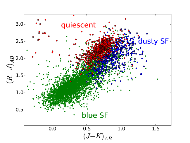
Figure 9: $(R-J)$ versus $(J-K)$ colour-colour diagram of $0.8\leq z\leq 0.95$ galaxies. Red points are quiescent galaxies, while green and blue points are SF galaxies with low ($E(B-V)<0.45$) and high ($E(B-V)\geq 0.45$) extinction, which are classified in our SED-fitting. The location of each type of galaxies in this diagram shows the reliability of galaxy type classification from our SED-fitting.

Figure 9 shows the location of galaxies with the photometric redshift, $0.8\leq z_{ph}\leq 0.95$, in the $(R-J)-(J-K)$ diagram, which corresponding to the rest-frame $UVJ$ diagram at this redshift range. In this figure, red and blue points are quiescent and dusty ($E(B-V)\geq 0.45$) SF galaxies classified in our SED-fitting. Figures 8 and 9 demonstrate the reliability of SED-fitting in classifying them as being star-forming or quiescent.

In L15, we have already shown that our SED-fitting (combined with the deep optical data) can distinguish between quiescent galaxies and dusty SF galaxies (Figure 3 in L15). Also, we checked the MIPS 24 $\micron$m detection of our sample galaxies using SpUDS MIPS catalog, finding that all 24 $\micron$m-detected galaxies are correctly classified as dusty SF galaxies based on our SED-fitting.

4 Spectroscopic Identification of Clusters/Groups at $z\sim 1$

4.1 Spectroscopically Identified Clusters/Groups

To identify galaxy clusters and groups from the spectroscopic data, we apply the following procedure.

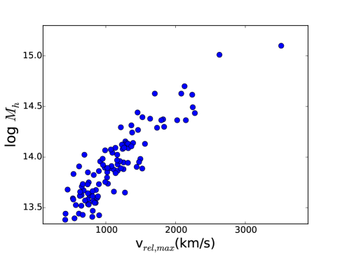
Figure 10: Correlation between the maximum rest-frame relative velocities (v_rel,max) of mock galaxy clusters from GALFORM simulation and their halo masses ($M_{h}$ in $M_{\odot}$). This shows that velocity cut of $\sim 3000$ km s^-1 is needed to properly detect and measure the velocity dispersions of galaxy clusters with their mass up to $\sim 10^{15}$ $M_{\odot}$.

First, from the spectroscopic redshift distribution of each cluster candidate, we discriminate galaxies as separate structures if the velocity gap (defined as the difference in the rest-frame velocities of galaxies adjacent in the velocity space) is larger than 1500 km/s. Next, for each separate structure, we apply 3-$\sigma$ clipping over the redshift distribution of cluster/group galaxy candidates to exclude obvious outliers. A tentative cluster/group redshift is determined to be the mean redshift of the remaining galaxies. Then, we further exclude any galaxies if their relative rest-frame velocity goes beyond $\pm$3000 km s^-1 from the cluster redshift. This velocity cut is set after investigating the correlation between the maximum rest-frame velocities and halo masses of mock galaxy clusters from the GALFORM simulation (Merson et al., 2013) (Figure 10). While we use a generous velocity cut of 3000 km s^-1, member galaxies of all confirmed clusters/groups are within $\pm$2000 km s^-1, except the one at $z\sim 1.3$ (we discuss about this structure in next section). And, for majority of the confirmed clusters/groups, rest-frame velocities of member galaxies are within $\pm$1000 km s^-1.

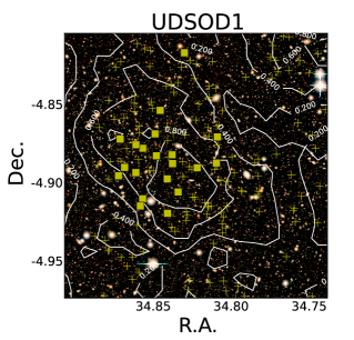
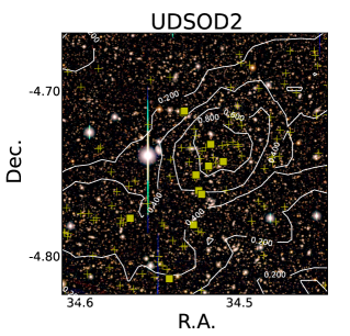
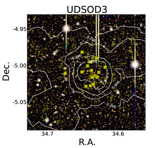
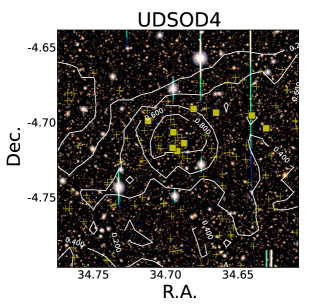
Figure 11: Composite colour ($R$,$i^{\prime}$,$z^{\prime}$) images of the confirmed overdensities. White contours show the galaxy surface number density levels, normalized to the maximum value in each region. Yellow squares show the locations of the spectroscopically confirmed members belonging to each overdensity, while photometrically identified member candidates as well as galaxies in the same photometric redshift range are shown with small yellow crosses. Each image tile size corresponds to $10\arcmin\times 10\arcmin$.

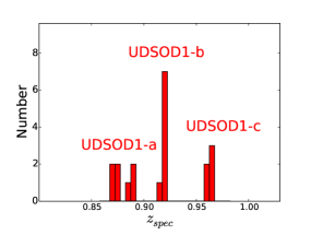
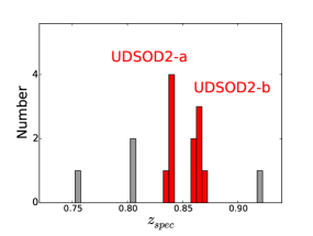
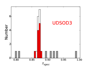
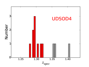
Figure 12: The spectroscopic redshift distribution of candidate member galaxies in the confirmed overdensities. The red bars are for the confirmed members of each overdensity, while the gray bars show galaxies that turned out to be outliers. The open bars show galaxies with a spectroscopic redshift from the literature.

Using this process, we confirm four candidates to contain significant overdensities that can be clusters/groups: three at $z\sim 0.9$ and one at $z\sim 1.3$. The colour composite images with the density contour of these overdensities are shown in Figure 11, and their spectroscopic redshift distributions are given in Figure 12. The redshift distribution shows that one cluster candidate, UDSOD1, is a system with three or four clusters/groups that are aligned along the line of sight, and another candidate, UDSOD2, is a system with two clusters/groups aligned along the line of sight. This kind of occurrence of multiple, spatially overlapped peaks within a single photometrically selected overdensity is also found in our test using the mock galaxy catalog from the GALFORM simulation (Merson et al., 2013) as shown in APPENDIX A, as well as in literature (e.g. van Breukelen et al., 2007, 2009)

UDSOD1, UDSOD2, and UDSOD3 have been identified as galaxy clusters or groups in F10 based on the extended X-ray emission and the red sequence of galaxies. Their counterparts in F10 are named as SXDF37XGG, SXDF21XGG, and SXDF46XGG. However, in F10, the number of $z_{spec}$ of member galaxies was small, 1 for UDSOD1, 0 for UDSOD2, and 6 for UDSOD3. Our spectroscopic observation unambiguously confirms their cluster nature and also reveals multiple peaks which can be separate structures along the line of sight. UDSOD4 stands as a newly discovered structure, not discussed in previous studies.

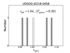
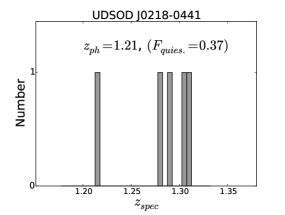
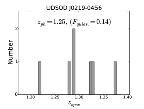
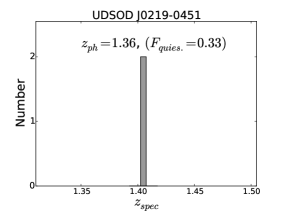
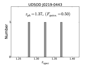
Figure 13: Distribution of spectroscopic redshift of unconfirmed cluster candidates. The open bar indicates galaxies with spectroscopic redshift from literature. We cannot confirm these candidates because of the small numbers of available redshifts.

For the other cluster candidates, the spectroscopic redshift distributions of candidate member galaxies are shown in Figure 13, and we find that the number of measured redshifts is too small to confirm them as clusters/groups. For the two cluster candidates at $z\sim 1.21$ and 1.25, four and three galaxies, are found to possibly form redshift peaks, out of five and seven redshift measured candidates, respectively. More spectroscopic data can tell whether they are truly clusters/groups in future. For the three remaining cluster candidates (one at $z\sim 1.0$ and two at $z\sim 1.4$), the numbers of spectroscopically confirmed galaxies are only four, two and three respectively. The cluster candidate at $z\sim 1.04$ is possibly an overlap of two structures: one at $z\sim 0.97$ and another at $z\sim 1.08$.

4.2 Properties of Spectroscopically Identified Galaxy Clusters/Groups

We describe the properties of the spectroscopically identified clusters/groups here. The derived properties are summarized in Table 2.

4.2.1 UDSOD1

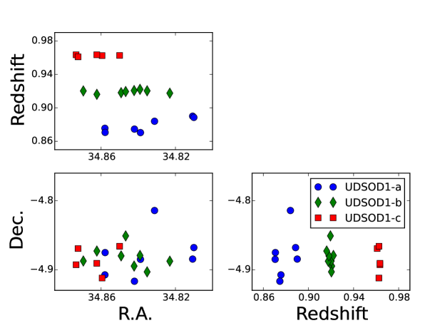
Figure 14: The three-dimensional distribution of three overdense structures belonging to UDSOD1. The blue circles, the green diamonds, and the red squares are the spectroscopically confirmed members of UDSOD1-a, UDSOD1-b, and UDSOD1-c, respectively. Among these three structures, UDSOD1-c shows a slight offset in its central position compared to UDSOD1-a and UDSOD1-b.

Using $z_{phot}$, this massive structure was initially identified as a single cluster candidate at $z\sim 0.89$ located at $\alpha\sim$ 02^h19^m22^s and $\delta$ = -4$\,{}^{\circ}$52$\arcmin$57$\arcsec$. Our spectroscopic observation of the member galaxy candidates has revealed that three to four overdensities are spatially overlapped. The upper left panel of Figure 12 shows the distribution of spectroscopic redshift of these overdensities at redshifts $z\sim 0.875$ (UDSOD1-a), 0.920 (UDSOD1-b), and 0.963 (UDSOD1-c) within a 2 Mpc projected radius circle from the group/cluster center. The velocity differences between peaks of each adjacent structure are about 7000 km s^-1. The number of spectroscopically confirmed members of these clusters/groups are seven (UDSOD1-a), eight (UDSOD1-b), and five (UDSOD1-c) within a 2 Mpc of projected radius from each group/cluster center. Among these, six (UDSOD1-a), eight (UDSOD1-b), and five (UDSOD1-c) are within a 1 Mpc projected radius from each group/cluster center. In Figure 14, we show the spatial distributions of these spectroscopically confirmed member galaxies. As can be seen in this figure, the spatial positions of the spectroscopic member galaxies of UDSOD1-a and UDSOD1-b are closely overlapped, while the members of UDSOD1-c are more concentrated on the eastern side.

We estimate the halo masses (throughout this paper, halo mass refers $M_{200}$ in most cases) from the total stellar masses within 1 Mpc, $M_{*,total}$, of these clusters/groups. To compute the total stellar mass, we use both the spectroscopically identified members and the member candidates based on the photometric redshift, but applying a weight, $w_{i}$, to each member candidate with $z_{phot}$ only. Here, $w_{i}$ is computed as the number of spectroscopically confirmed members divided by the sum of the numbers of spectroscopic members and outliers. When a cluster candidate turns out to be spatially overlapped multiple structures based on spectroscopic redshifts, galaxies belong to different structures are considered as outliers — e.g., spectroscopically identified members of UDSOD1-b and UDSOD1-c are considered as outliers in calculating $w_{i}$ for UDSOD1-a. For the spectroscopically confirmed members, this weight value is 1. Then, the total stellar mass is computed as

$$M_{*,total}=\Sigma w_{i}\times M_{*,i},$$ (1)

where log $M_{*,i}\geq 9.1$.

Galaxies whose photometric redshifts are in the range of $z_{cl}\pm 0.023\times(1+z_{cl})$ are included in this calculation.

The $M_{*,total}$ values are found to be $4.8\times 10^{11}$ M_⊙, $2.3\times 10^{11}$ M_⊙, and $3.5\times 10^{10}$ M_⊙ for UDSOD1-a, UDSOD1-b, and UDSOD1-c, respectively, and their values are listed in Table 3. From the calibration between $M_{200}$ and $M_{*,total}$ derived from our model test (APPENDIX B), $M_{200}$’s are estimated as $4.8\times 10^{13}$ M_⊙, $2.3\times 10^{13}$ M_⊙, and $3.5\times 10^{12}$ M_⊙, each. In case of UDSOD1-a, the redshift distribution is made of two peaks, with the velocity gap to be about 1200 km s^-1. If UDSOD1-a is considered as two groups, their $M_{*,total}$’s are $9.6\times 10^{10}$ M_⊙ and $2.0\times 10^{11}$ M_⊙, giving the stellar-mass–calibrated $M_{200}$ as $9.6\times 10^{12}$ M_⊙ and $2.0\times 10^{13}$ M_⊙, each.

In Table 3, we summarize the derived properties of the UDSOD1 and other overdensities presented below. The X-ray-based $M_{200}$ of UDSOD1 is available with the value of $9.3\times 10^{13}$ M_⊙ (SXDF37XGG; F10). This value is in a reasonable agreement with $M_{200}$ from $M_{*,total}$ with UDSOD1-a as a single structure. Note that there was only one $z_{spec}$ available in F10 for SXDF37XGG with $z_{spec}=0.845$ which was suggested as the redshift of the structure. With our $z_{spec}$, we suggest that the redshift of the structure should be revised to either $z_{spec}=0.875$ of UDSOD1-a or $z_{spec}=0.920$ of UDSOD1-b.

From the stellar-mass–calibrated $M_{200}$, we estimate $R_{200}$ using the following relation (e.g., Kim et al., 2016).

$$R_{200}=10^{-2/3}\frac{G^{1/3}}{H(z)^{2/3}}M_{200}^{1/3},$$ (2)

where $H(z)$ is the Hubble parameter at redshift $z$.

Then we also calculated $F_{q}$, the quiescent fraction of each overdensity, within $R_{200}$. Like $M_{*,total}$, we used both spectroscopic members and photometric members and adopted the same weights, $w_{i}$, to compute $F_{q}$. The large fraction of member galaxies in the overdensities UDSOD1-a, UDSOD1-b, and UDSOD1-c are actively forming stars with a quiescent galaxy fraction ($F_{q}$) of $\sim 0.09$, 0.27, and 0.00, respectively.

4.2.2 UDSOD2

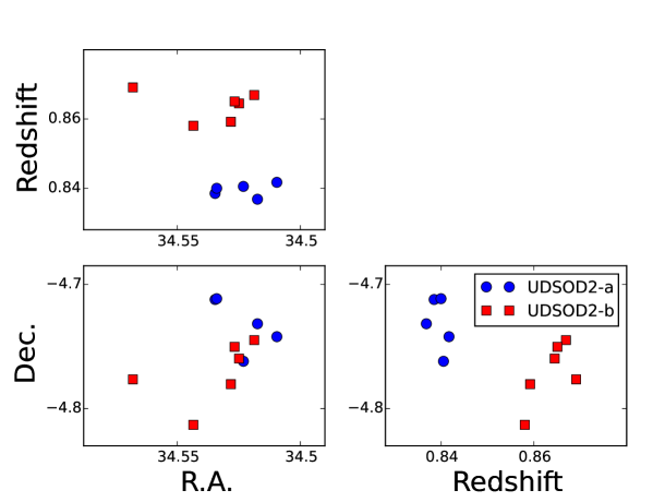
Figure 15: The three dimensional distribution of two overdense structures belonging to UDSOD2. The blue circles and the red squares are the spectroscopically confirmed members of UDSOD2-a and UDSOD2-b, respectively.

The redshift distribution of UDSOD2 candidate galaxies within 2 Mpc from the overdensity center is shown in the upper right panel in Figure 12. For this cluster candidate, we identify two significant redshift peaks at $z=0.840$ (UDSOD2-a with 6 spectroscopic redshift members) and 0.865 (UDSOD2-b with 5 spectroscopic redshift members), and the velocity gap between the peaks of these two structures is $\sim 4000$ km s^-1. As shown in Figure 15, the spatial distributions of member galaxies of these two structures overlap with each other to some degree, while UDSOD2-b is more extended toward the south-east.

We find that the total stellar masses of $2.8\times 10^{11}$ M_⊙ and $4.8\times 10^{11}$ M_⊙ for UDSOD2-a and UDSOD2-b respectively, which translate into $M_{200}$ of $2.8\times 10^{13}$ M_⊙ and $4.8\times 10^{13}$ M_⊙ each based on our $M_{200}-M_{*,total}$ calibration. The derived values of $M_{200}$ of UDSOD2-b, the main structure, or the sum of the masses of the two substructures, agree well with the X-ray derived $M_{200}$ of $1.0\times 10^{14}$ M_⊙ (SXDF21XGG; F10). Note that there is no $z_{spec}$ available for this structure in F10, and their redshift of $z=0.860$ is based on $z_{phot}$. Our redshift measurement suggests that this structure is made of two peaks at $z_{spec}=0.840$ and 0.865. We also find that these overdensities have an intermediate $F_{q}$ among galaxy cluster candidates at $0.85<z<0.9$, of 0.44 and 0.53.

4.2.3 UDSOD3

This overdensity shows the highest quiescent galaxy fraction among three target galaxy cluster candidates at $z\sim 0.87$. Eleven galaxies (out of 18 candidates) are spectroscopically confirmed to be the members of this overdensity from our Magellan observation. In addition, there are five galaxies that are members of this cluster based on the spectroscopic redshifts from the literature (Smail et al., 2008; Simpson et al., 2012; Akiyama et al., 2015). The spectroscopic redshift distribution of these galaxies is shown in the lower left panel of Figure 12, and we determine its redshift to be $z=0.8731$.

We find that $M_{*,total}$ of this overdensity is $1.0\times 10^{12}$ M_⊙, and stellar-mass calibrated $M_{200}$ is $1.0\times 10^{14}$ M_⊙. The X-ray based $M_{200}$ is $1.4\times 10^{14}$ M_⊙ (SXDF46XGG; F10), in agreement with the $M_{200}$ values we derived. The halo mass estimates suggest that this overdensity can be classified as a low mass cluster. Note that F10 determined $z_{spec}$ of this structure to be $z=0.875$ based on six $z_{spec}$ measurements, which agrees well with our redshift determination. The quiescent fraction of this overdensity is found to be 0.51.

4.2.4 UDSOD4

This overdensity is at a higher redshift, $z=1.294$, than the above three overdensities. Within a 2 Mpc (1 Mpc) projected radius, there are nine (seven) galaxies whose redshifts are measured and confirmed as the overdensity members. The redshift distribution is shown in the lower right panel of Figure 12.

As can be seen in Figure 12, the redshift distribution of this cluster has a red wing. The two galaxies at $z\sim 1.32$ are separated by $\sim 1300$ km s^-1 from the other seven members. If we apply a tighter velocity gap of 1200 km s^-1 to identify cluster/group members, these two galaxies will be excluded. The total stellar mass and stellar-mass calibrated $M_{200}$ are $1.0\times 10^{12}$ M_⊙ and $1.0\times 10^{14}$ M_⊙. We suggest that this overdensity is either a cluster or group with M${}_{halo}\sim 10^{14}$ M_⊙, although no X-ray counterpart to this structure was identified. The quiescent galaxy fraction is 0.40, which is intermediate among three $z\sim 1.3$ targets.

5 Extended Overdense Structures

Besides identifying galaxy clusters/groups, we have also searched for LSSs around the spectroscopically identified clusters/groups, combining the spectroscopic redshifts from our Magellan observation and those from the literature (Smail et al., 2008; Simpson et al., 2012; Akiyama et al., 2015). Through this search, we find extended LSSs, with sizes (physical scales) of up to $\sim 10$ Mpc, around three overdensities (UDSOD1, UDSOD2, and UDSOD4), while no significant extended LSS is found near UDSOD3.

5.1 Large-scale Structure near UDSOD1-a

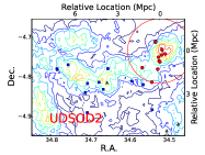
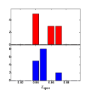
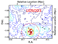
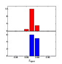
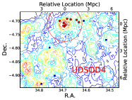
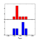
Figure 16: Galaxy density map in the regions near the galaxy clusters/groups: (Upper left) near UDSOD1-a, (Upper right) near UDSOD2, (Lower left) near UDSOD3, and (Lower right) near UDSOD4. Galaxies with only photometric redshift are also included in the galaxy number density measurement shown as contours. The red filled circles and blue squares show galaxies whose spectroscopic redshifts are measured from our Magellan observation. The red filled circles are the members of each cluster whose location is shown as the red large open circle in each figure. The blue squares are galaxies whose spectroscopic redshifts are within the spectroscopic redshift range of each cluster. The green triangles indicate galaxies with spectroscopic redshifts taken from the literature. The large red circles enclose the overdensities within 2 Mpc projected radius. Relative locations (from cluster center) are given in physical scales. The red and blue histograms in each panel show the spectroscopic redshift distributions of overdensity members and non-members, respectively.

Contours in the upper left panel of Figure 16 show the galaxy surface number density near UDSOD1-a within a narrow redshift bin. The galaxy surface number density is measured by combining spectroscopic as well as photometric redshifts. For galaxies with photometric redshift only, we include galaxies whose redshifts are within the range, $|\Delta z|/(1+z_{cl})\leq 0.023$, where $z_{cl}$ is the redshift of UDSOD1-a. For galaxies with spectroscopic redshift, we include galaxies whose spectroscopic redshifts are within the redshift range of UDSOD1-a, of $0.87\leq z\leq 0.89$. The UDSOD1-a is at the bottom left region of this density map.

Interestingly, we find an extended LSS in the western side of UDSOD1-a with a scale of $\sim 8$ Mpc. There are also several dense, group-like, structures along this LSS, including the ones at ($\alpha,\delta$) $\sim$ (34$\,{}^{\circ}$.74, $-4\,^{\circ}$.80) and (34$\,{}^{\circ}$.62, $-4\,^{\circ}$.77). Although the density contours are constructed using mostly galaxies with photometric redshifts, galaxies with spectroscopic redshifts follow the density contour closely, lending credibility to the association of the LSS to UDSOD1-a. We note that UDSOD1-b and UDSOD1-c show similar LSSs around them, and we suggest that the UDSOD1-a through c are all a part of a single LSS.

5.2 Large-scale Structure near UDSOD2

We also find an extended LSS near UDSOD2, as shown in the upper right panel of Figure 16, which extends up to $\sim 10$ Mpc. The UDSOD2 is in the top right region. In this figure, we show the spectroscopically confirmed member galaxies of UDSOD2-a and UDSOD2-b together, as red circles, since the velocity interval between the redshifts of UDSOD2-a and UDSOD2-b is about 4000 km s^-1, or 30 Mpc on the physical scale, indicating these two structures may belong to a single LSS. For galaxies with only a photometric redshift, we include those within $|\Delta z|/(1+z_{cl,mean})\leq 0.023$ to construct the density contour. Here, $z_{cl,mean}$ is the mean redshift of UDSOD2-a and UDSOD2-b. Over 20 galaxies with spectroscopic redshifts in a similar range as UDSOD2 are distributed in the filamentary structure toward the east side of UDSOD2.

5.3 Large-scale Structure near UDSOD3

UDSOD3 is relatively isolated without no significant LSSs near it, as can be seen in the lower left panel of Figure 16. This shows a sharp contrast to the other overdensities at a similar redshift.

5.4 Large-scale Structure near UDSOD4

In the lower right panel of Figure 16, we show the LSS around UDSOD4, which is at $z\sim 1.3$. Not many spectroscopic redshifts are available around UDSOD4, but the density map from the photometric redshift sample suggests an association of UDSOD4 with extended intermediate density regions over 3-5 Mpc from cluster UDSOD4.

6 Connection between SF Activities in Clusters and LSSs

In Figure 1, we have shown that there is a large variation in the quiescent galaxy fraction among individual galaxy cluster candidates even though they reside at a similar redshift. Here, we investigate if the cluster SF activities are linked to LSSs. We concentrate our analysis on galaxy clusters/groups with log($M_{200}/M_{\odot}$) $\geq 13.4$. The overdensities that satisfy this condition are UDSOD1-a, b, UDSOD2-a, b, UDSOD3 and UDSOD4.

6.1 Enhancement of SF Activity in Galaxy Overdensities near LSSs

In Section 5, we presented the extended LSSs around galaxy overdensities, UDSOD1-a, UDSOD2, and UDSOD4, with scales as large as $\sim 10$ Mpc. On the other hand, there is no significant extended LSS around UDSOD3 — i.e., this overdensity is relatively isolated. Interestingly, galaxy overdensities that are embedded in the extended LSSs appear to show a higher fraction of SF galaxies among members, compared to the relatively isolated galaxy overdensity.

To quantify this large-scale environmental trend, we measure the fraction of the area covered by the extended LSSs within 10 Mpc around each galaxy cluster using the friends-of-friends (FOF) method. We study the LSSs within 10 Mpc, based on our finding of LSSs with sizes of $\sim 10$ Mpc as presented in Section 5. First, we select the sky area around each galaxy cluster within a projected radius of 10 Mpc and within the survey boundary and divide the area into cells with a size of $12\arcsec\times 12\arcsec$. Next, we measure galaxy number counts in each cell within the redshift range of $|\Delta z|/(1+z_{cl})\leq 0.023$. Then, we find overdense cells with a number count greater than 2-$\sigma$ from the mean background count. Finally, we mark the connected overdense cells with a linking length of 2 Mpc using the FOF algorithm.

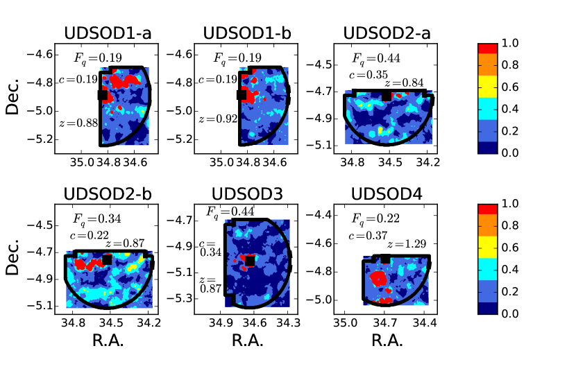
Figure 17: Distribution of overdense ($\geq 2\sigma$) LSSs near confirmed galaxy overdensities (shown as red region). Thick black line in each panel shows the boundary which encloses the total area. The boundary is set by either 10 Mpc projected radius or the survey boundary. These connected structures are found using the friend-of-friend (FOF) algorithm. Coloured contours show the normalized galaxy surface number density levels. Here, similarly as in density maps (Figure 16), we can see that UDSOD3 is relatively isolated, unlike the other confirmed overdensities at a similar redshift, such as UDSOD1-a and UDSOD2-b. In each panel, we show the quiescent fraction ($F_{q}$), redshift, and the concentration parameter ($c$) of each cluster.

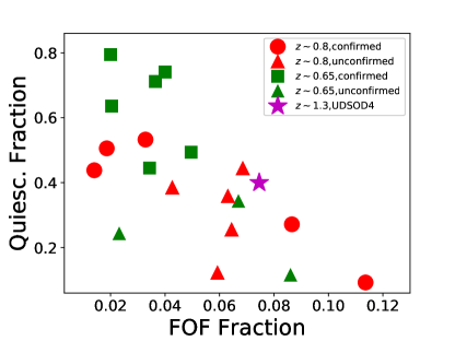
Figure 18: Correlation between the fraction of the area covered by the overdense region connected with cluster ($x$-axis) and the quiescent galaxy fraction ($y$-axis). The red circles show the values for spectroscopically studied overdensities at $z\sim 0.8$ from this work, and the red triangles are for cluster candidates at a similar redshift. The green triangles and green squares show the values of cluster candidates at a lower redshift ($z\sim 0.65$). Among these, green squares are for $z\sim 0.65$ candidates confirmed in other works (van Breukelen et al., 2006; Galametz et al., 2018). The magenta star shows the value of UDSOD4, which is at $z=1.29$. The FOF fraction and the quiescent fraction show anti-correlation. We do not include UDSOD1-c because of its very small mass ($\sim 10^{12}$ M_⊙).

The results are shown in Figure 17 for the confirmed overdensities with log(M₂₀₀/M${}_{\odot})>13.4$. In this figure, the thick black line in each panel shows the boundary which encloses the total area. This boundary is set by either 10 Mpc projected radius from each overdensity (whose center is shown with the black square) or by the survey boundary. The red-coloured region shows the connected LSS found. Here, we can see that UDSOD2-a and UDSOD3 are relatively isolated while the other overdensities are surrounded with extended LSSs. The fraction of the area covered by the extended LSS (red region) within the total area (gray area) — ‘FOF fraction’ — is 0.11, 0.09, 0.01, 0.03, 0.02, and 0.08 for UDSOD1-a, UDSOD1-b, UDSOD2-a, UDSOD2-b, UDSOD3, and UDSOD4, respectively. Note that we did not make a correction for the region where no data are available. As shown with the red circles and the purple star in Figure 18, there is a strong anti-correlation between the FOF fraction and the $F_{q}$, with the Pearson correlation coefficient of -0.89.

We test if this FOF fraction is a reliable tracer of actual LSSs by checking if the FOF fractions from random distribution of galaxies have low values. We find that the median number of galaxies in a photometric redshift slice is about 500 within 10 Mpc projected radius circle for our sample galaxies. Therefore, we distribute 500 points randomly within 10 Mpc projected radius circle, then calculate FOF fraction following the same procedure explained in the above paragraph. We repeat this procedure 100 times, and find that FOF fractions are smaller than 0.01 in all cases.

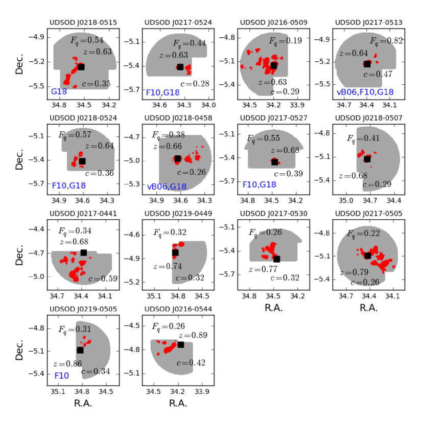
Figure 19: Distribution of the overdense ($\geq 2\sigma$) large scale structures (shown as red regions) near galaxy cluster candidates at $0.55<z<0.9$. Gray region shows the total area whose boundary is set by either 10 Mpc projected radius or the survey boundary. These connected structures are found using the friend-of-friend (FOF) algorithm. In each panel, we show the quiescent fraction ($F_{q}$), redshift, and the concentration parameter ($c$) of each cluster. Some of our candidates are detected are detected in X-ray and their halo mass estimated with the X-ray data (F10) or spectroscopically confirmed in other works (van Breukelen et al., 2006; Galametz et al., 2018, vB06; G18), and the references are shown in each panel.

Encouraged by this trend, we also analyzed the LSSs around 16 other cluster candidates with log $(M_{200}/M_{\odot})>13.4$ at $0.55<z<0.9$ in the UDS field from L15. Note that 6 out of these 16 candidates have been identified as clusters or groups either spectroscopically or through X-ray detection. These cluster candidates are listed in Table 4 along with their associated properties. We choose this redshift range since the photometric redshift uncertainty is relatively small ($|\Delta z|$/$(1+z)$ = 0.017), and the overdensity identification has been proven to be secure even with photometric redshifts only (this work and others, e.g., Lai et al., 2016) in this redshift range. We show the large-scale environment around these cluster candidates in Figure 19. The $F_{q}$ as a function of the FOF fraction is shown in Figure 18, where the red triangles and the green symbols are the cluster candidates at $0.7<z<0.9$ and at $0.55<z<0.7$, respectively. With this larger set of data, we confirm the anti-correlation between the quiescent galaxy fraction of galaxy clusters and the FOF fraction.

We test the significance of this correlation using the Pearson test. The Pearson correlation coefficient, $r$ is $-0.76$ for $z\sim 0.85$ samples of clusters and cluster candidates, indicating strong anti-correlation. For $z\sim 0.65$ cluster candidates, $r=-0.63$. This trend remains even if the samples from the two redshift ranges are combined, although in general, the lower redshift sample tends to have higher $F_{q}$ for a given FOF-fraction.

Note that the use of the photometric resdhift cut could include foreground and background structures which are not actually at the same distance with the overdensity. Depending on whether these foreground or background structures are connected with the central overdensity (in the photometric redshift slice), this could overestimate or underestimate the FOF fractions. Therefore, we check this using mock galaxy catalog from Merson et al. (2013), by comparing the FOF fractions computed from two methods: one using galaxies in a narrow physical distance ($\pm$ 20 Mpc) from the cluster center, and another using galaxies from the photometric redshift cut ($\pm$ 0.023$\times(1+z)$) as we did for the simulation (see APPENDIX A) that would include galaxies out to $\pm$ 100 Mpc from the cluster center in comoving distance.

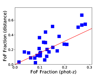
Figure 20: Correlation between FOF fraction of mock clusters measured based on photometric redshift ($x$-axis) and physical radial distance ($y$-axis). These two quantities show a good positive correlation inferring the reliability of measuring FOF fraction using photometric redshift. The red line shows the line where [FoF Fraction (photo-z)]/[FoF Fraction (distance)] = 0.64, which is the median value of this ratio.

Figure 20 shows the comparison between FOF fractions of mock clusters measured using the sample from the ‘photometric redshift’ cut and the sample with the ‘physical distance’ cut. This figure shows the FOF fractions from the two methods show a positive correlation with the rms scatter of 0.60, but the photometric redshift based FOF fraction being somewhat underestimated by a factor of $\sim 0.64$. The underestimate in the FOF fraction for the photometric redshift cut sample can be understood as the following. More galaxies are included in the photometric redshift cut sample, and this increases the number density fluctuation, $\sigma$. Due to this increase in $\sigma$, the area above the 2-$\sigma$ fluctuation threshold decreases, leading to the underestimation of the FOF fraction.

6.2 Dependence of SF Activity of Galaxy Clusters on Halo Concentration

Simulations show the growth of overdense areas in connection to LSSs of filaments (e.g., Ebeling et al., 2004). Under this kind of scenario, isolated galaxy clusters like UDSOD3 are the ones that get disconnected from the LSS and finish its dynamical evolution early. Then, we can expect that clusters like them are virialized and more concentrated as they evolve further in an isolated environment.

We investigate the correlation between the quiescent galaxy fraction and the concentration of galaxy distribution of the confirmed overdensities and cluster candidates with log (M₂₀₀/M${}_{\odot})\geq 13.4$. For this, we define the concentration parameter of the galaxy overdensity as ‘$-$log ($A_{0.3}/A_{0.7}$)’, where $A_{0.3}$ and $A_{0.7}$ are the areas that contain $30\%$ and $70\%$ of the total member galaxies.

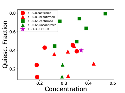
Figure 21: Correlation between concentration of galaxy clusters ($x$-axis) and quiescent galaxy fraction ($y$-axis). The symbol assignments are the same as Figure 18.

Figure 21 shows the correlation between the concentration parameter and the quiescent fraction of various overdensities. The correlation between $F_{q}$ and concentration is weak with the Pearson coefficient of 0.61, mainly due to three outliers with a low $F_{q}$ and a high concentration at $z\sim 0.8$ and $z\sim 1.3$. However, if we remove these three points, the correlation becomes stronger (Pearson coefficient $\sim 0.70$). The same is true if we focus on the four galaxy overdensities at $z\sim 0.8$. We conclude that at a given redshift, there seems to be a correlation between $F_{q}$ and concentration of galaxy overdensities, although a larger sample of spectroscopically confirmed samples is needed to reach a firm conclusion.

6.3 Web-feeding Model of SF in Overdensities at $z\sim 1$

Based on the correlation of the quiescent galaxy fraction with two parameters, the FOF fraction of the surrounding LSS and the concentration parameter of the overdensity, we suggest the “Web-feeding model” to explain the variety of SF activities in clusters at $z\sim 1$. In the model, we attribute the enhanced SF activities in overdensities are due to the inflow of gas and SF galaxies to localized overdense areas (Fadda et al., 2008; Mahajan et al., 2012; Pintos-Castro et al., 2013; Darvish et al., 2014; Hayashi et al., 2017; Kleiner et al., 2017). The concentration parameter of overdensities stays low in such regions due to new SF galaxies filling up the outskirt of galaxy overdensities even if overdensity members in-fall to the overdensity center. However, once the supply of gas and galaxies stops, i.e., LSS around the overdensities disappears, SF activity of the overdensity stops and the overdensities become concentrated with continued in-fall of member galaxies toward their centers. This picture can explain the observed association of the LSS with low $F_{q}$ overdensities and the possible high concentration of overdensities with high $F_{q}$. This scenario is consistent with the CWD model (Aragon-Calvo et al., 2019).

The biased galaxy formation, where galaxies formed earlier in higher density regions connected to LSSs, could work against our finding. Despite of this opposite effect of the biased galaxy formation working on the LSS-$F_{q}$ connection, the fact that we find the anti-correlation between the FOF fraction and $F_{q}$ suggests that the Web-feeding effect could be stronger than what is found here.

7 Summary and Conclusion

In this paper, we present the results of the MOS observation of high redshift ($0.8<z<1.3$) galaxy cluster candidates in the UDS field. Based on the spectroscopic observation and the photometric redshifts, we investigate whether SF galaxy fraction in overdense areas is enhanced due to the presence of adjacent LSSs. The results are summarized below.

1. We identify four high-redshift ($0.8<z<1.3$) galaxy overdensities, containing 7 to 8 clusters/groups of galaxies. The spectroscopically identified clusters/groups are found to have halo masses in the range of $13\lesssim$ log ($M_{200}/M_{\odot}$) $\lesssim 14$.

2. We also find elongated LSSs near three confirmed galaxy overdensities, which extend as large as 10 Mpc. The LSSs are found from the photometric redshift sample, but spectroscopically confirmed galaxies also follow the distribution of LSSs.

3. There is an anti-correlation between the quiescent galaxy fraction in clusters/groups and the significance of the surrounding LSS. The significance of LSSs is quantified using the FOF algorithm, expressed as the ‘FOF fraction’. This finding indicates that SF activity in galaxy overdensities is enhanced when the overdensities at $z\sim 1$ are surrounded by LSSs.

4. We find that more concentrated overdensities tend to have a higher quiescent galaxy fraction, with some exceptions. However this trend needs to be confirmed with a larger set of data in the future.

5. Based on the results 3 and 4, we put forward the “Web-feeding model” for SF activities in overdensities at $z\sim 1$. In this model, the low $F_{q}$ of overdensities surrounded by LSS can be explained with inflow of gas and SF galaxies from the surrounding LSSs into the overdensities. Once the supply of the gas and galaxies stops and the surrounding LSS disappears, galaxy overdensities become filled with quiescent galaxies that infall to cluster center producing the high concentration of overdensities.

Our results show that SF activities in galaxy overdensities at $0.55<z<1.3$ with $13.4\lesssim$ log ($M_{200}/M_{\odot}$) $\lesssim 14$ are closely connected with the presence of LSSs. Future spectroscopy study of dense sampling of galaxies over a much larger area should reveal much clearer picture about the proposed connection between SF activity in clusters/groups and LSSs surrounding them.

Appendix A Selection of Massive Structures based on Photometric Data

There are several methods used to find massive structures of galaxies (e.g., galaxy clusters) at high redshift. Among these, the selection method based on photometric redshift is an efficient way, especially considering increasing number of panchromatic photometric surveys (e.g., Trevese et al., 2007; Eisenhardt et al., 2008; Kang & Im, 2015; Lee et al., 2015; Kim et al., 2016). Here, we test if this kind of photometric selection of massive structures is reliable — i.e., how many photometrically-found overdensities are actually clusters or groups.

For this, we use the mock galaxy catalog of Merson et al. (2013). From the mock catalog, we select four sky areas, each of which has a similar sky area with the UDS field. Then we add noise to the spectroscopic redshift of each galaxy with the amount of the photometric redshift error from the observed data (see Figure 6) assuming Gaussian distribution. From this mock ‘photometric redshift’ catalog, we select overdensities following the same procedure as the one explained in Section 2.1 and also in L15.

After identifying overdensities, we check the spectroscopic redshift distribution of each overdensity, finding $95\%$ of the photometrically selected overdensities contain massive structures like galaxy clusters or groups.

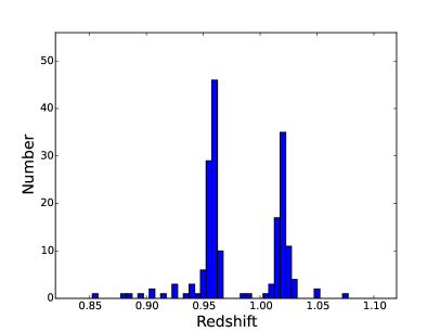
Figure 22: An example of the spectroscopic redshift distribution of a photometrically selected mock overdensity from the mock photometric redshift catalog. $49\%$ of photometrically selected model overdensities contain multiple peaks in their spectroscopic redshift distribution.

From this test, we also find that about half ($\sim 49\%$) of photometrically found overdensities contain multiple peaks in their spectroscopic redshift distribution as shown in Figure  22. The existence of spatially overlapped multiple structures within a single photometrically selected overdensity is found in our sample as well (with a similar occurrence fraction), and also often found in other studies as well (e.g. van Breukelen et al., 2007, 2009).

Appendix B Simulation Test of Correlation between Halo Mass and Total Stellar Mass

Studies show that there exists a tight correlation between the mass of dark matter halos of clusters or groups and the total stellar mass of cluster/group member galaxies (e.g., Kim et al., 2015; Patel et al., 2015; Lin et al., 2017; Kravtsov et al., 2018). Here, we check this correlation in model halos in the similar ways as used for our observationally selected clusters/groups. The mock catalogs in APPENDIX A are used here. For each model halo, we first select galaxies within the photometric redshift error range. Then, among these galaxies, fifteen galaxies are randomly selected, and we check if these galaxies are cluster members or not. For these fifteen galaxies, we derive the weight, $w_{i}$, to be the number of member galaxies divided by fifteen. Then we calculate the total stellar mass applying this weight. We repeat this procedure 1000 times, and use the median stellar mass from these 1000 run in the following analysis.

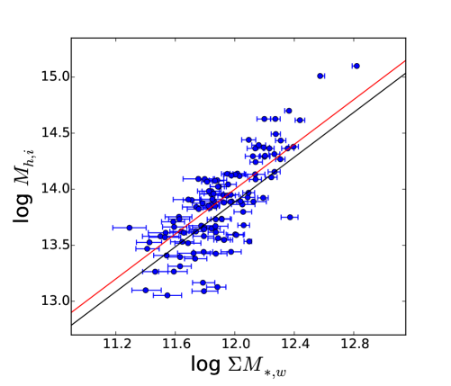
Figure 23: Correlation between halo mass and the total stellar mass of overdensities found from the mock catalog. The total stellar mass is calculated using the same procedure done for analyzing observed overdensities (Section 4.2). The red line is the line with log ($M_{halo}/M_{*,total}$)=2.0, while the black line shows the correlation between halo mass and total stellar mass from L15.

The Figure 23 shows that the total stellar mass is proportional to the halo mass. The error bars in the figure show the scatter (the first and third quartiles) in the measured total stellar mass for each halo from 1000 Monte Carlo runs. The median value of these scatters is 0.06 (same for both upper and lower scatter) in logarithmic scale. The median and the rms scatter of log ($M_{halo}/M_{*,total}$) are 2.00 and 0.25. The scatter of the median value of log ($\Sigma M_{*,i}$) is much smaller than the rms scatter in log ($M_{halo}/M_{*,total}$), and can be considered negligible when converting $M_{*,total}$ to $M_{halo}$.

The scatter in the $M_{halo}-M_{*,total}$ correlation is modest, which is well consistent with other studies (Patel et al., 2015; Kravtsov et al., 2018). The black line in this figure shows $M_{*,total}$ to $M_{200}$ ratio of 0.013 found in L15.

This correlation between $M_{*,total}$ and $M_{200}$ of clusters/groups indicates that $M_{*,total}$ can be a good proxy for cluster/group mass (Andreon et al., 2012). Therefore, in Section 4.2, we provide $M_{200}$ values converted from the total stellar mass, applying the above mentioned best-fit correlation. The dispersion in the correlation and scatter in $M_{*,total}$ from the Monte Carlo runs are also included (as a quadrature) in the error budget of $M_{200}$ (column (9) in Table 3).

Table 1: Overdensity targets

Name	$z_{phot}$	$z_{spec}$ measured/targetsa
UDSOD1b,d	0.89	20/24
UDSOD2b,d	0.89	15/16
UDSOD3b,d	0.87	18/22
UDSOD4b,d	1.24	12/15
UDSOD J0218-0441b,e	1.21	5/6
UDSOD J0219-0456b,e	1.25	7/9
UDSOD J0218-0458c,e	1.04	4/12
UDSOD J0219-0451c,e	1.36	2/6
UDSOD J0219-0443c,e	1.37	3/7

Table 2: Target UDS Galaxies for our Magellan spectroscopic observation

ID	R.A. (J2000)	dec. (J2000)	$z_{spec}$	$flag$	$z_{phot}$	$R_{AB}$	Cluster ID
(1)	(2)	(3)	(4)	(5)	(6)	(7)	(8)
UDS-228531	34.64690	-5.04229	—	—	0.865	24.49	—
UDS-229694	34.64075	-5.03853	0.8116	b	0.918	24.47	—
UDS-231087	34.64948	-5.03574	—	—	0.848	23.97	—
UDS-234710	34.63850	-5.02716	0.8743	b	0.832	23.34	3
UDS-235482	34.63426	-5.02524	0.8753	b	0.855	23.73	3
UDS-235622	34.63008	-5.02307	0.8972	b	0.833	24.49	—
UDS-236426	34.63672	-5.02090	0.7986	a	0.819	23.27	—
UDS-236747	34.60576	-5.01930	0.9114	b	0.871	23.90	—
UDS-238512	34.63570	-5.01564	0.8723	b	0.884	23.06	3
UDS-238531	34.62882	-5.01538	0.8772	b	0.910	23.38	3
UDS-239219	34.64142	-5.01153	—	—	0.826	24.47	—
UDS-239439	34.63197	-5.01353	0.8750	a	0.881	22.79	3
UDS-240385	34.65060	-5.00833	0.8779	b	0.857	24.25	3
UDS-240908	34.62673	-5.00883	0.8693	b	0.853	23.22	3
UDS-241334	34.63706	-5.00619	0.8745	b	0.830	24.42	3
UDS-243040	34.66692	-5.00251	0.9298	b	0.882	23.11	—
UDS-243163	34.60729	-5.00077	—	—	0.911	23.17	—
UDS-244398	34.60018	-4.99799	—	—	1.004	23.80	—
UDS-245018	34.63802	-4.99461	0.8676	a	0.836	23.37	3
UDS-246462	34.64983	-4.99181	0.9884	b	0.875	24.00	—
UDS-247109	34.63007	-4.98942	0.8710	b	0.839	23.68	3
UDS-249003	34.58368	-4.98388	—	—	1.056	24.13	—
UDS-249146	34.64603	-4.98557	0.9176	a	0.866	23.35	—
UDS-249702	34.65040	-4.98120	0.8604	b	0.887	24.36	3
UDS-249779	34.58160	-4.98399	—	—	1.061	23.30	—
UDS-251072	34.59115	-4.98098	—	—	1.055	22.86	—
UDS-253772	34.59892	-4.97094	—	—	1.069	24.48	—
UDS-254106	34.75435	-4.96990	1.2354	b	1.199	23.36	—
UDS-254869	34.74907	-4.96749	1.2904	b	1.239	23.33	—
UDS-254902	34.59714	-4.96754	1.0806	a	1.018	23.32	—
UDS-254980	34.59380	-4.96865	—	—	1.012	23.19	—
UDS-255098	34.61484	-4.96656	—	—	1.016	24.00	—
UDS-256270	34.78955	-4.96476	—	—	1.286	23.48	—
UDS-256378	34.61165	-4.96365	—	—	1.020	24.37	—
UDS-256643	34.59917	-4.96423	—	—	1.016	22.18	—
UDS-257227	34.57320	-4.96207	—	—	1.015	23.94	—
UDS-258072	34.69135	-4.95880	0.8733	a	0.851	23.28	—
UDS-260259	34.77536	-4.95349	0.7928	b	0.821	22.68	—
UDS-260634	34.57821	-4.95170	0.9808	b	0.998	24.41	—
UDS-261211	34.80573	-4.94992	—	—	1.297	23.98	—
UDS-261778	34.55985	-4.94946	0.8751	b	0.834	22.67	—
UDS-262504	34.72490	-4.94716	1.2915	b	1.182	22.32	—
UDS-263004	34.80919	-4.94550	—	—	1.253	24.02	—
UDS-263423	34.51558	-4.94456	0.8735	b	0.875	22.82	—
UDS-264476	34.83005	-4.94270	—	—	1.214	23.20	—
UDS-265946	34.56188	-4.93772	0.9607	b	0.913	23.3	—
UDS-266173	34.78123	-4.93566	0.9268	b	0.932	23.38	—
UDS-267294	34.75909	-4.93306	1.3241	b	1.242	23.33	—
UDS-267966	34.78945	-4.93104	1.2904	b	1.225	23.58	—
UDS-268909	34.82768	-4.92870	—	—	1.273	23.69	—
UDS-269070	34.54436	-4.92888	1.0589	b	1.024	22.84	—
UDS-270063	34.83935	-4.92447	1.2794	b	1.221	24.17	—
UDS-270445	34.76143	-4.92622	0.7905	a	0.832	21.85	—
UDS-271576	34.82034	-4.92197	1.2185	b	1.252	23.80	—
UDS-271680	34.53366	-4.92030	1.1026	b	1.021	23.48	—
UDS-272156	34.69100	-4.91928	1.2817	b	1.213	23.31	—
UDS-272637	34.52046	-4.91798	—	—	1.233	23.21	—
UDS-272659	34.82060	-4.91882	1.3764	b	1.231	23.56	—
UDS-272708	34.84207	-4.91679	0.8746	a	0.873	24.11	1-a
UDS-273396	34.78667	-4.91462	1.3325	b	1.305	24.37	—
UDS-274407	34.85949	-4.91211	0.9624	b	0.928	23.59	1-c
UDS-274524	34.53860	-4.91359	0.8754	a	0.877	22.98	—
UDS-275441	34.51866	-4.90938	0.9622	b	0.899	22.87	—
UDS-275596	34.71127	-4.90992	0.9299	b	0.863	23.12	—
UDS-276058	34.85797	-4.90754	0.8756	b	0.894	23.35	1-a
UDS-276882	34.53532	-4.90534	1.2711	b	1.199	23.42	—
UDS-277386	34.68735	-4.90490	0.9217	b	0.923	22.62	—
UDS-277731	34.73405	-4.90280	1.2312	b	1.181	23.26	—
UDS-277735	34.83523	-4.90318	0.9204	b	0.910	24.17	1-b
UDS-277802	34.51316	-4.90243	0.8698	b	0.842	23.27	—
UDS-278440	34.73294	-4.90075	1.2842	b	1.216	23.34	—
UDS-279317	34.85374	-4.89782	1.4026	b	1.331	23.48	—
UDS-279506	34.71846	-4.89810	1.0416	b	1.020	23.06	—
UDS-280301	34.84224	-4.89478	0.9207	b	0.886	23.65	1-b
UDS-281576	34.87351	-4.89281	0.9634	b	0.940	23.30	1-c
UDS-281951	34.86235	-4.89081	0.9634	b	0.923	22.53	1-c
UDS-282637	34.82302	-4.88770	0.9175	b	0.908	23.69	1-b
UDS-282670	34.52402	-4.88735	1.2808	b	1.169	23.37	—
UDS-282683	34.70849	-4.88985	0.8510	b	0.994	22.96	—
UDS-282725	34.86685	-4.89073	—	—	0.924	23.37	—
UDS-283427	34.86960	-4.88744	0.9202	b	0.923	23.38	1-b
UDS-283892	34.83882	-4.88500	0.8704	a	0.839	22.13	1-a
UDS-284432	34.86063	-4.88256	—	—	0.869	22.97	—
UDS-284464	34.81072	-4.88463	0.8900	a	0.901	22.84	1-a
UDS-284743	34.54264	-4.88225	0.8488	a	0.889	23.17	—
UDS-285335	34.69280	-4.88131	0.8866	b	0.814	23.13	—
UDS-285442	34.84924	-4.88002	0.9181	b	0.865	23.41	1-b
UDS-285528	34.82124	-4.88199	—	—	0.923	23.87	—
UDS-286367	34.84731	-4.87751	1.4033	b	1.378	23.62	—
UDS-286518	34.83908	-4.87939	0.9221	b	0.879	22.41	1-b
UDS-286588	34.73166	-4.87695	0.9712	b	0.927	23.12	—
UDS-287242	34.85786	-4.87521	0.8707	b	0.845	23.62	1-a
UDS-287852	34.86231	-4.87299	0.9161	b	0.873	23.19	1-b
UDS-287888	34.84760	-4.87508	—	—	1.331	23.51	—
UDS-288765	34.71830	-4.87180	—	—	0.928	22.93	—
UDS-288805	34.86459	-4.87180	—	—	0.854	23.07	—
UDS-289121	34.87242	-4.86937	0.9610	b	0.937	22.23	1-c
UDS-289271	34.81006	-4.86798	0.8886	b	0.887	24.03	1-a
UDS-290427	34.71991	-4.86649	0.9266	b	0.874	23.15	—
UDS-290579	34.85003	-4.86603	0.9626	a	0.930	22.49	1-c
UDS-291394	34.86009	-4.86516	—	—	0.914	22.97	—
UDS-291643	34.70777	-4.86344	1.3939	b	1.374	21.90	—
UDS-292029	34.84612	-4.86106	—	—	1.301	23.93	—
UDS-292229	34.85287	-4.86294	—	—	1.349	23.75	—
UDS-292371	34.74278	-4.86118	1.0560	a	1.034	23.25	—
UDS-295775	34.84679	-4.85103	0.9195	b	0.894	23.98	1-b
UDS-295803	34.75636	-4.85083	0.9310	b	0.925	23.22	—
UDS-296910	34.67932	-4.84771	1.0094	b	0.901	23.28	—
UDS-298584	34.86310	-4.84316	—	—	1.392	23.97	—
UDS-299358	34.64368	-4.84205	—	—	0.842	23.38	—
UDS-300797	34.71334	-4.83955	0.8411	b	0.862	22.50	—
UDS-301305	34.70603	-4.83559	—	—	1.082	23.47	—
UDS-303047	34.66753	-4.83115	0.8478	a	0.846	22.69	—
UDS-303667	34.72319	-4.82904	1.0554	b	1.021	22.75	—
UDS-303953	34.55543	-4.82916	1.0770	a	0.998	23.46	—
UDS-304202	34.62020	-4.82734	1.1809	b	1.064	23.05	—
UDS-304566	34.51992	-4.82607	1.1561	b	1.024	22.65	—
UDS-304585	34.71726	-4.82676	—	—	1.229	22.84	—
UDS-305878	34.58210	-4.82342	0.7772	a	0.830	23.24	—
UDS-306056	34.70878	-4.82250	1.0189	b	1.008	23.08	—
UDS-306573	34.70792	-4.81634	0.8679	b	0.835	21.70	—
UDS-307198	34.56587	-4.81928	0.8401	b	0.790	22.88	—
UDS-307542	34.71526	-4.81900	1.3859	b	1.365	23.37	—
UDS-308248	34.83765	-4.81644	0.9634	b	0.937	23.33	—
UDS-308415	34.57049	-4.81708	1.0523	b	0.999	23.25	—
UDS-309250	34.54344	-4.81307	0.8580	b	0.838	22.97	2-b
UDS-309800	34.83124	-4.81421	0.8840	b	0.925	23.49	1-a
UDS-309849	34.82151	-4.81154	0.8251	a	0.842	22.63	—
UDS-310171	34.67828	-4.81322	0.8456	b	0.813	21.01	—
UDS-310820	34.86150	-4.80826	0.9019	b	0.901	23.43	—
UDS-310841	34.59476	-4.81040	0.8677	b	0.806	22.64	—
UDS-310952	34.65653	-4.80873	—	—	0.833	23.20	—
UDS-312133	34.54492	-4.80747	0.8408	a	0.813	22.66	—
UDS-313589	34.58816	-4.80331	1.0986	b	1.073	23.18	—
UDS-313974	34.87246	-4.80101	0.8316	b	0.880	23.14	—
UDS-314141	34.59129	-4.79898	0.8572	b	0.869	23.47	—
UDS-314225	34.70618	-4.80062	1.0504	b	1.203	23.02	—
UDS-314832	34.85776	-4.79807	0.8761	b	0.884	23.10	—
UDS-314889	34.75458	-4.79716	1.3178	b	1.215	23.42	—
UDS-315323	34.64763	-4.79703	1.0831	b	1.068	23.48	—
UDS-316538	34.53368	-4.79317	0.8825	a	0.870	22.26	—
UDS-316584	34.72644	-4.79254	0.8343	a	0.881	23.15	—
UDS-316613	34.71928	-4.79456	0.8719	b	0.900	23.35	—
UDS-316643	34.87366	-4.79501	—	—	0.883	23.37	—
UDS-317085	34.83352	-4.79248	1.1513	b	1.179	23.34	—
UDS-317860	34.76135	-4.78958	1.4576	b	1.369	23.26	—
UDS-318479	34.62929	-4.79089	1.0854	b	1.256	23.11	—
UDS-318699	34.66456	-4.78748	1.2713	b	1.176	22.63	—
UDS-319198	34.87153	-4.78745	—	—	1.014	22.67	—
UDS-319682	34.60902	-4.78522	0.8878	b	0.842	22.11	—
UDS-320687	34.78495	-4.78144	0.8509	b	0.867	23.25	—
UDS-321054	34.62932	-4.78077	—	—	0.813	23.48	—
UDS-321110	34.52822	-4.78036	0.8592	a	0.794	22.34	2-b
UDS-321367	34.65572	-4.77906	0.8463	a	0.864	22.96	—
UDS-322051	34.78581	-4.77935	0.8503	b	0.888	22.31	—
UDS-322278	34.67725	-4.77674	1.0833	b	1.011	23.30	—
UDS-322652	34.84634	-4.77655	1.0497	a	1.018	22.85	—
UDS-323047	34.56600	-4.77644	0.8691	a	0.798	22.23	2-b
UDS-323500	34.70461	-4.77254	0.8722	b	0.862	23.50	—
UDS-324211	34.59881	-4.77360	0.8804	a	0.822	21.93	—
UDS-324306	34.84994	-4.77155	1.0475	b	0.936	23.26	—
UDS-324514	34.63706	-4.76977	—	—	1.034	23.49	—
UDS-324868	34.53780	-4.77107	0.9555	a	0.915	22.78	—
UDS-325191	34.75730	-4.76932	0.8425	b	0.801	22.81	—
UDS-325205	34.51362	-4.76841	1.3110	b	1.229	23.28	—
UDS-325328	34.52161	-4.76845	0.8049	b	0.791	23.46	—
UDS-325804	34.61840	-4.76758	0.8812	a	0.862	22.99	—
UDS-325951	34.81144	-4.76622	0.9325	a	0.903	23.39	—
UDS-326679	34.72874	-4.76341	1.1899	b	1.197	23.31	—
UDS-326940	34.66651	-4.76529	0.9734	b	0.850	22.58	—
UDS-327832	34.80331	-4.76028	0.8255	a	0.814	22.53	—
UDS-328018	34.64759	-4.76059	0.8805	a	0.834	22.79	—
UDS-328084	34.52312	-4.76191	0.8405	a	0.872	22.79	2-a
UDS-328399	34.52490	-4.75969	0.8645	b	0.851	22.72	2-b
UDS-329293	34.63724	-4.75814	0.8811	b	0.850	22.77	—
UDS-330370	34.53937	-4.75354	0.7551	a	0.792	22.20	—
UDS-330393	34.56446	-4.75353	—	—	1.007	23.25	—
UDS-332031	34.54285	-4.75128	—	—	0.875	23.46	—
UDS-332415	34.52670	-4.75025	0.8651	a	0.809	22.32	2-b
UDS-332893	34.82824	-4.74734	1.2810	b	1.350	24.49	—
UDS-333517	34.84335	-4.74426	1.3698	b	1.335	24.00	—
UDS-334546	34.50953	-4.74210	0.8417	a	0.869	23.66	2-a
UDS-334552	34.51872	-4.74485	0.8669	b	0.885	22.54	2-b
UDS-334823	34.82278	-4.74166	—	—	1.393	24.47	—
UDS-334863	34.53096	-4.74227	—	—	0.816	22.37	—
UDS-338191	34.71060	-4.73169	1.3557	b	1.267	23.43	—
UDS-338315	34.51740	-4.73168	0.8368	b	0.825	23.34	2-a
UDS-339117	34.69383	-4.72919	1.4038	b	1.260	23.21	—
UDS-339310	34.85504	-4.72769	—	—	1.307	24.39	—
UDS-339814	34.85943	-4.72999	0.8893	b	1.406	24.02	—
UDS-340102	34.52670	-4.72659	—	—	0.809	24.26	—
UDS-340421	34.55467	-4.72521	0.8046	a	0.797	23.08	—
UDS-341240	34.66593	-4.72263	—	—	1.297	24.11	—
UDS-341435	34.78862	-4.72228	0.8246	a	0.817	23.22	—
UDS-341894	34.52547	-4.72222	—	—	0.793	23.21	—
UDS-342357	34.70268	-4.72055	1.3611	b	1.180	23.48	—
UDS-343198	34.85323	-4.71673	1.3258	b	1.302	24.14	—
UDS-343250	34.69148	-4.71830	1.2943	b	1.190	23.34	4
UDS-343777	34.53057	-4.71615	0.9203	b	0.877	24.45	—
UDS-343860	34.69462	-4.71620	1.2901	a	1.182	22.63	4
UDS-344737	34.70541	-4.71390	—	—	1.213	23.67	—
UDS-344878	34.68667	-4.71312	1.2927	b	1.225	22.61	4
UDS-345732	34.53461	-4.71216	0.8385	b	0.815	22.67	2-a
UDS-345854	34.53396	-4.71149	0.8400	b	0.808	21.93	2-a
UDS-346190	34.82927	-4.71146	—	—	1.339	24.48	—
UDS-346271	34.69253	-4.71137	—	—	1.255	23.39	—
UDS-346514	34.66734	-4.71027	—	—	1.240	23.76	—
UDS-346705	34.76465	-4.70954	0.8204	b	0.829	22.51	—
UDS-346750	34.65765	-4.70804	—	—	1.184	23.52	—
UDS-347025	34.79855	-4.70749	0.9009	b	0.864	22.60	—
UDS-347036	34.69412	-4.70580	1.3135	b	1.285	23.92	4
UDS-348003	34.62996	-4.70317	1.2905	b	1.233	23.80	4
UDS-348269	34.79899	-4.70331	0.9604	b	0.926	22.66	—
UDS-349053	34.78108	-4.70123	0.9602	b	1.193	23.18	—
UDS-349372	34.59794	-4.70021	—	—	1.247	24.45	—
UDS-349733	34.71157	-4.69821	1.2940	b	1.233	23.79	4
UDS-350345	34.60964	-4.69812	1.3077	b	1.237	24.29	—
UDS-350773	34.75123	-4.69593	0.9204	b	0.890	23.42	—
UDS-351328	34.63979	-4.69460	1.3034	b	1.257	23.46	4
UDS-352105	34.66459	-4.69271	1.3205	b	1.237	23.17	4
UDS-352892	34.68014	-4.69021	1.2823	b	1.183	23.18	4
UDS-354242	34.74165	-4.68610	0.8992	a	0.895	23.16	—
UDS-354710	34.76780	-4.68804	0.9003	a	0.898	22.16	—
UDS-355005	34.61463	-4.68410	1.2174	b	1.236	24.22	—
UDS-358074	34.61502	-4.67741	1.2778	b	1.216	23.84	—
—	34.82014	-4.81893	0.0000	star	—	16.88a	—
—	34.65724	-4.94467	0.0000	star	—	15.78a	—

Note. —

(1) Galaxy ID.

(2) R.A. in degree.

(3) Declination in degree.

(4) Spectroscopic redshift.

(5) Quality flag (a: multiple features, b: single feature).

(6) Photometric redshift.

(7) Subaru $R$-band magnitude.

(8) Cluster/group membership.

Table 3: Properties of galaxy clusters/groups

Name	R.A. (J2000)	dec. (J2000)	$z_{cl}$	$ProjectedRadius$	$N_{spec}$	$w_{i}$	log ($M_{*,total}$)	log $M_{200}$	$N_{g}$	$F_{quies.}$	$R_{200}$	$Concent.$
(1)	(2)	(3)	(4)	(5)	(6)	(7)	(8)	(9)	(10)	(11)	(12)	(13)
UDSOD1-a	34.84044	-4.88481	$0.8751\pm 0.0080$	1.0	6	—	—	—	—	—	—	—
—	—	—	—	2.0	7	0.35	11.7	$13.7\pm 0.3$	43	0.09	540	0.19
UDSOD1-a1	—	—	—	1.0	4	0.20	11.0	$13.0\pm 0.3$	9	0.16	—	—
UDSOD1-a2	—	—	—	2.0	3	0.15	11.3	$13.3\pm 0.3$	12	0.26	—	—
UDSOD1-b	34.84452	-4.88373	$0.9198\pm 0.0018$	1.0	8	0.40	11.4	$13.4\pm 0.3$	11	0.27	420	0.19
UDSOD1-c	34.86235	-4.89081	$0.9626\pm 0.0009$	1.0	5	0.25	10.5	$12.5\pm 0.3$	6	0.00	220	0.27
UDSOD2-a	34.52312	-4.73168	$0.8400\pm 0.0017$	1.0	5	0.33	11.4	$13.4\pm 0.3$	11	0.44	460	0.35
UDSOD2-b	34.52580	-4.75497	$0.8648\pm 0.0029$	1.0	4	—	—	—	—	—	—	—
—	—	—	—	1.5	6	0.40	11.7	$13.7\pm 0.3$	22	0.53	540	0.22
UDSOD3	34.63638	-5.00953	$0.8731\pm 0.0045$	1.0	11(16)a	0.61	12.0	$14.0\pm 0.3$	56	0.51	690	0.34
UDSOD4	34.69148	-4.70580	$1.2940\pm 0.0126$	1.0	7	—	—	—	—	—	—	—
—	—	—	—	2.0	9	0.75	12.0	$14.0\pm 0.3$	59	0.40	590	0.37
UDSOD4b	—	—	—	2.0	7	0.58	11.7	$13.7\pm 0.3$	24	0.27	—	—

Note. —

(1) Galaxy cluster name.

(2) R.A. in degree.

(3) Declination in degree.

(4) Cluster Redshift.

(5) Projected radius in Mpc.

(6) Number of galaxies with spectroscopic redshift within the projected radius indicated in column (5).

(7) Weight computed as the number of spectroscopically confirmed members divided by the sum of the numbers of spectroscopic members and outliers.

(8) Total stellar mass (in M_⊙).

(9) Halo mass calibrated from the correlation between total stellar mass and halo mass of model clusters derived in Appendix B (in M_⊙).

(10) Number of member galaxies corrected by applying weights for photo-$z$ selected members (see text for detailed explanation).

(11) Quiescent galaxy fraction within $R_{200}$ (applying weights for photo-$z$ members).

(12) Halo radius calculated from $M_{200}$ (in kpc).

(13) Halo Concentration.

Table 4: Properties of galaxy cluster candidates

Name	$z_{phot}$	log $M_{200}$	$z_{spec}$	log $M_{200}$	Other Names
			(G18)	(F10)
(1)	(2)	(3)	(4)	(5)	(6)
UDSOD J0218-0515	0.626	13.9	0.6453	—	C2c
UDSOD J0217-0524	0.629	13.7	0.6451	13.9	SXDF08XGGb,U9c
UDSOD J0216-0509	0.633	13.8	—	—	—
UDSOD J0217-0513	0.639	14.1	0.6470	14.2	1Aa,SXDF69XGGb,C1c
UDSOD J0218-0524	0.644	14.0	0.6459	14.0	SXDF07XGGb,U2c
UDSOD J0218-0458	0.659	13.6	0.6476	—	3a,U3c
UDSOD J0217-0527	0.677	14.0	0.6937	13.8	SXDF04XGGb,U1Nc
UDSOD J0218-0507	0.684	13.7	—	—	—
UDSOD J0217-0441	0.685	13.5	—	—	—
UDSOD J0219-0449	0.744	13.4	—	—	—
UDSOD J0217-0530	0.774	13.6	—	—	—
UDSOD J0217-0505	0.791	13.8	—	—	—
UDSOD J0219-0505	0.865	13.8	—	13.9	SXDF52XGGb
UDSOD J0216-0544	0.889	13.8	—	—	—

Note. —

(1) Name.

(2) Photometric redshift.

(3) Halo mass calibrated from total stellar mass.

(4) Spectroscopic redshift from G18.

(5) Halo mass from F10.

(6) Other names from various references.

References

- Aihara et al. (2018) Aihara, H. et al. 2018, PASJ, 70, S4
- Akiyama et al. (2015) Akiyama, M. et al. 2015, PASJ, 67,82
- Alberts et al. (2014) Alberts, S. et al. 2014, MNRAS, 437, 437
- Alberts et al. (2016) Alberts, S. et al. 2016, ApJ, 825,72
- Almaini et al. (2007) Almaini, O. et al. 2007, ASP Conf. Ser. Vol. 379, Cosmic Frontiers. Astron. Soc. Pac., San Francisco, p. 163
- Andreon et al. (2012) Andreon, S. 2012, A&A, 548, A83
- Aragon-Calvo et al. (2019) Aragon-Calvo, M. A., Neyrinck, M. C., & Silk, J. 2019, The Open Journal of Astrophysics, 2, 7
- Bai et al. (2009) Bai, L., Rieke, G. H., Rieke, M. J., Christlein, D. and Zabludoff, A. I. 2009, ApJ, 693, 1840
- Baldry et al. (2006) Baldry, I. K. et al. 2006, MNRAS, 373, 469
- Bamford et al. (2009) Bamford, S. P., Nichol, R. C., & Baldry, I. K. et al. 2009, MNRAS, 393, 1324
- Blanton et al. (2005) Blanton, M. R., Eisenstein, D., Hogg, D. W., Schlegel, D. J., & Brinkmann, J. 2005, ApJ, 629, 143
- Brammer et al. (2008) Brammer, G. B., van Dokkum, P. G., & Coppi, P. 2008, ApJ, 686, 1503
- Brodwin et al. (2013) Brodwin, M., Stanford, S. A., & Gonzalez, A. H. et al. 2013, ApJ, 779, 138
- Butcher & Oemler (1984) Butcher, H. & Oemler, A. Jr. 1984, ApJ, 285, 426
- Chabrier (2003) Chabrier, G. 2003, PASP, 115, 763
- Cooke et al. (2016) Cooke, E. A., Hatch, N. A., Stern, D. et al. 2016, ApJ, 816, 83
- Cooper et al. (2008) Cooper, M. C., et al. 2008, MNRAS, 383, 1058
- Cooper et al. (2012) Cooper, M. C., Griffith, R. L., & Newman, J. A. et al. 2012, MNRAS, 419, 3018
- Darvish et al. (2014) Darvish, B., Sobral, D., & Mobasher, B. et al. 2014, ApJ, 796, 51
- Dressler et al. (2011) Dressler, A. et al. 2011, PASP, 123, 288
- Ebeling et al. (2004) Ebeling, H., Barrett, E. & Donovan, D. 2004, ApJ, 609, L49
- Eisenhardt et al. (2008) Eisenhardt, P. R. M. et al. 2008, ApJ, 684, 905
- Elbaz et al. (2007) Elbaz, D., et al. 2007, A&A, 468, 33
- Ellingson et al. (2001) Ellingson, E., Lin, H., Yee, H. K. C. and Carlberg, R. G. 2001, ApJ, 547, 609
- Fadda et al. (2008) Fadda, D., Biviano, A., Marleau, F. R., Storrie-Lombardi, L. J., & Durret, F. 2008, ApJ, 672, L9
- Finoguenov et al. (2010) Finoguenov, A. et al. 2010, MNRAS, 403, 2063 (F10)
- Galametz et al. (2018) Galametz, A. et al. 2018, MNRAS, 475, 4148 (G18)
- Geach et al. (2011) Geach, J. E., Ellis, R. S., Smail, I., Rawle, T. D. & Moran, S. M. 2011, MNRAS, 413, 177
- Hayashi et al. (2017) Hayashi, M. et al. 2017, ApJ, 841, L21
- Hayashi et al. (2019) Hayashi, M. et al. 2019, PASJaccepted, preprint(arXiv: 1905.13437)
- Hayashi et al. (2011) Hayashi, M., Kodama, T., Koyama, Y., Tadaki, K.-I. and Tanaka, I. 2011, MNRAS, 415, 2670
- Im et al. (1997) Im, M., Griffiths, R. E. & Ratnatunga, K. U. 1997, ApJ, 475, 457
- Jian et al. (2018) Jian, H.-Y. et al. 2018, PASJ, 70, S23
- Kang & Im (2015) Kang, E. & Im, M. 2015, JKAS, 48, 21
- Kauffmann et al. (2004) Kauffmann, G., et al. 2004, MNRAS, 353, 713
- Kim et al. (2015) kim, J.-W., Im, M., & Lee, S.-K. et al. 2015, ApJ, 806, 189
- Kim et al. (2016) kim, J.-W., Im, M., & Lee, S.-K. et al. 2016, ApJ, 821, L10
- Kleiner et al. (2017) Kleiner, D., Pimbblet, K. A., Jones, D. H., Koribalski, B. S. & Serra, P. 2017, MNRAS, 466, 4692
- Ko et al. (2012) Ko, J., Im, M., Lee, H. M. et al. 2012, ApJ, 745, 181
- Koyama et al. (2008) Koyama, Y., Kodama, T., Shimasaku, K. et al. 2008, MNRAS, 391, 1758
- Koyama et al. (2018) Koyama, Y. et al. 2018, PASJ, 70, S21
- Kravtsov et al. (2018) Kravtsov, A. V. and Vikhlinin, A. A. and Meshcheryakov, A. V. 2018, Astronomy letters, 44, 8
- Lai et al. (2016) Lai, C.-C., Lin, L., Jian, H.-Y. et al. 2016, ApJ, 825, 40
- Lee et al. (2010) Lee, S.-K., Ferguson, H. C., Somerville, R. S., Wiklind, T., & Giavalisco, M. 2010, ApJ, 725, 1644
- Lee et al. (2015) Lee, S.-K., Im, M., & Kim, J.-W. et al. 2015, ApJ, 810, 90 (L15)
- Lemaux et al. (2012) Lemaux, B. C. et al. 2012, ApJ, 745, 106
- Lewis et al. (2002) Lewis, I. et al. 2002, MNRAS, 334, 673
- Lin et al. (2017) Lin, Y.-T. et al. 2017, ApJ, 851, 139
- Lubin et al. (2009) Lubin, L. M., Gal, R. R., Lemaux, B. C., Kocevski, D. D. & Squires, G. K. 2009, AJ, 137, 4867
- Mahajan et al. (2012) Mahajan, S., Raychaudhury, S. & Pimbblet, K. A. 2012, MNRAS, 427, 1252
- Masters & Capak (2011) Masters, D. & Capak, P. 2011, PASP, 123,638
- Merson et al. (2013) Merson, A. I. et al. 2013, MNRAS, 429, 556
- Muzzin et al. (2012) Muzzin, A., Wilson, G., & Yee, H. K. C. et al. 2012, ApJ, 746, 188
- Oke (1974) Oke, J. B. 1974, ApJS, 27, 21
- Papovich et al. (2012) Papovich, C., Bassett, R., & Lotz, J. M. et al. 2012, ApJ, 750, 93
- Patel et al. (2009) Patel, S. G., Holden, B. P., Kelson, D. D., Illingworth, G. D., & Franx, M. 2009, ApJ, 705, L67
- Patel et al. (2015) Patel, S. G. et al. 2015, ApJ, 799, L17
- Peng et al. (2010) Peng, Y.-J., Lilly, S. J., Kovač, K., et al. 2010, ApJ, 721, 193
- Pintos-Castro et al. (2013) Pintos-Castro, I., Sánchez-Portal, M., Cepa, J. et al. 2013, A&A, 558, A100
- Quadri et al. (2012) Quadri, R. F., Williams, R. J., Franx, M., & Hildebrandt, H. 2012, ApJ, 744, 88
- Saintonge et al. (2008) Saintonge, A., Tran, K.-V. H. and Holden, B. P., 2008, ApJ, 685, L113
- Scoville et al. (2013) Scoville, N., Arnouts, S., & Aussel, H. et al. 2013, ApJS, 206, 3
- Shimakawa et al. (2018) Shimakawa, R. et al. 2018, MNRAS, 473, 1977
- Simpson et al. (2012) Simpson, C. et al. 2012, MNRAS, 421, 3060
- Smail et al. (2008) Smail, I., Sharp, R., Swinbank, A. M., Akiyama, M., Ueda, Y., Foucaud, S., Almaini, O. & Croom, S. 2008, MNRAS, 389, 407
- Strazzullo et al. (2013) Strazzullo, V., Gobat, R., & Daddi, E., et al. 2013, ApJ, 772, 118
- Tran et al. (2010) Tran, K.-V. H. et al. 2010, ApJ, 719, L126
- Tran et al. (2005) Tran, K.-V. H., van Dokkum, P., Illingworth, G. D., Kelson, D., Gonzalez, A. & Franx, M. et al. 2005, ApJ, 619, 134
- Trevese et al. (2007) Trevese, D., Castellano, M., Fontana, A. & Giallongo, E. 2007, A&A, 463, 853
- van Breukelen et al. (2006) van Breukelen, C. et al. 2006, MNRAS, 363, L26 (vB06)
- van Breukelen et al. (2007) van Breukelen, C. et al. 2007, MNRAS, 382, 971
- van Breukelen et al. (2009) van Breukelen, C. et al. 2009, MNRAS, 395, 11
- van der Burg et al. (2013) van der Burg, R. F. J., Muzzin, A., & Hoekstra, H. et al. 2013, A&A, 557, A15
- Webb et al. (2013) Webb, T. M. A. et al. 2013, AJ, 146, 84
- Yoon et al. (2017) Yoon, Y., Im, M., & Kim, J.-W. 2017, ApJ, 834, 73