On Dyakonov–Voigt surface waves guided by the planar interface of dissipative materials

Abstract

Dyakonov–Voigt (DV) surface waves guided by the planar interface of (i) material ${\cal A}$ which is a uniaxial dielectric material specified by a relative permittivity dyadic with eigenvalues $\varepsilon^{s}_{\cal A}$ and $\varepsilon^{t}_{\cal A}$, and (ii) material ${\cal B}$ which is an isotropic dielectric material with relative permittivity $\varepsilon_{\cal B}$, were numerically investigated by solving the corresponding canonical boundary-value problem. The two partnering materials are generally dissipative, with the optic axis of material ${\cal A}$ being inclined at the angle $\chi\in\left[0^{\circ},90^{\circ}\right]$ relative to the interface plane. No solutions of the dispersion equation for DV surface waves exist when $\chi=90^{\circ}$. Also, no solutions exist for $\chi\in\left(0^{\circ},90^{\circ}\right)$, when both partnering materials are nondissipative. For $\chi\in\left[0^{\circ},90^{\circ}\right)$, the degree of dissipation of material ${\cal A}$ has a profound effect on the phase speeds, propagation lengths, and penetration depths of the DV surface waves. For mid-range values of $\chi$, DV surface waves with negative phase velocities were found. For fixed values of $\varepsilon^{s}_{\cal A}$ and $\varepsilon^{t}_{\cal A}$ in the upper-half-complex plane, DV surface-wave propagation is only possible for large values of $\chi$ when $|\varepsilon_{\cal B}|$ is very small.

1 Introduction

This paper concerns the propagation of electromagnetic surface waves [1, 2, 3] guided by the planar interface of two dissimilar materials labeled ${\cal A}$ and ${\cal B}$. Both partnering materials are homogeneous and dielectric. The relative permittivity dyadic $\underline{\underline{\varepsilon}}_{\cal A}$ of material ${\cal A}$ is uniaxial [4] with eigenvalues $\varepsilon^{s}_{\cal A}$ and $\varepsilon^{t}_{\cal A}$. Material ${\cal B}$ is isotropic with relative permittivity scalar $\varepsilon_{\cal B}$. It has been established very well, both theoretically [5, 6] and experimentally [7, 8, 9], that this interface supports the propagation of Dyakonov surface waves, for certain ranges of values of $\varepsilon^{s}_{\cal A}$, $\varepsilon^{t}_{\cal A}$, and $\varepsilon_{\cal B}$.

In contrast to surface-plasmon-polariton waves [10, 11], for example, Dyakonov surface waves propagate without decay when both partnering materials are nondissipative [12, 13, 14, 15]. Typically, Dyakonov surface waves propagate only for a small range of directions parallel to the interface plane [12, 16]; but much larger ranges of directions are possible, if partnering materials are dissipative [17, 18], magnetic [19], or exhibit negative-phase-velocity plane-wave propagation [20].

As we established recently [21], the planar interface of materials ${\cal A}$ and ${\cal B}$ can support another type of surface wave, namely the Dyakonov–Voigt (DV) surface wave. There are fundamental differences between DV surface waves and Dyakonov surface waves: The amplitude of a DV surface wave decays in a combined exponential–linear manner with increasing distance from the interface plane in material ${\cal A}$, whereas Dyakonov surface waves only decay in an exponential manner with inceasing distance from the interface plane. Furthermore, a DV surface wave propagates in only one direction in each quadrant of the interface plane whereas Dyakonov surface waves propagate for a range of directions in each quadrant of the interface plane [12, 13].

The fields of the DV surface wave in the partnering material ${\cal A}$ have similar characteristics to the fields associated with a singular form of planewave propagation called Voigt-wave propagation [22]. The existence of a Voigt wave for an unbounded anisotropic material is a consequence of the corresponding propagation matrix being non-diagonalizable [23, 24, 25, 26]. The feature that distinguishes a Voigt wave from a conventional plane wave [4, 27] is that the Voigt wave’s amplitude depends on the product of an exponential function of the propagation distance and a linear function of the propagation distance, the latter being absent for a conventional plane wave.

DV surface-wave propagation has been established [21] when both partnering materials and nondissipative and the optic axis of material ${\cal A}$ lies wholly in the interface plane. In the following sections, DV surface-wave propagation is investigated for the case where the partnering materials are generally dissipative and the optic axis of material ${\cal A}$ is inclined at the angle $\chi$ relative to the interface plane. As we demonstrate, the incorporation of dissipation and inclination of the optic axis of material ${\cal A}$ has profound effects upon the phase speeds, propagation lengths, and penetration depths of the DV surface waves.

In the notation adopted, the permittivity and permeability of free space are denoted by $\varepsilon_{\scriptscriptstyle 0}$ and $\mu_{\scriptscriptstyle 0}$, respectively. The free-space wavelength is written as $\lambda_{\scriptscriptstyle 0}=2\pi/k_{\scriptscriptstyle 0}$ with $k_{\scriptscriptstyle 0}=\omega\sqrt{\varepsilon_{\scriptscriptstyle 0}\mu_{\scriptscriptstyle 0}}$ being the free-space wavenumber and $\omega$ being the angular frequency. The real and imaginary parts of complex-valued quantities are delivered by the operators $\mbox{Re}\left\{\mbox{ \tiny{${}^{\bullet}$} }\right\}$ and $\mbox{Im}\left\{\mbox{ \tiny{${}^{\bullet}$} }\right\}$, respectively, and $i=\sqrt{-1}$. Single underlining denotes a 3-vector and $\left\{\hat{\underline{u}}_{x},\hat{\underline{u}}_{y},\hat{\underline{u}}_{z}\right\}$ is the triad of unit vectors aligned with the Cartesian axes. Square brackets enclose matrixes and column vectors. The superscript ^T denotes the transpose. The complex conjugate is denoted by an asterisk.

2 Theory

2.1 Preliminaries

In the canonical boundary-value problem for DV surface-wave propagation shown in Fig. 1, material ${\cal A}$ occupies the half-space $z>0$ and material ${\cal B}$ the half-space $z<0$. The relative permittivity dyadic of material ${\cal A}$ is given as

$$\underline{\underline{\varepsilon}}_{\cal A}=\underline{\underline{S}}_{y}(\chi)\mbox{ \tiny{${}^{\bullet}$} }\left[{\varepsilon}_{\cal A}^{t}\hat{\underline{u}}_{x}\,\hat{\underline{u}}_{x}+{\varepsilon}_{\cal A}^{s}\left(\hat{\underline{u}}_{y}\,\hat{\underline{u}}_{y}+\hat{\underline{u}}_{z}\,\hat{\underline{u}}_{z}\right)\right]\mbox{ \tiny{${}^{\bullet}$} }\underline{\underline{S}}_{y}^{T}(\chi),$$ (1)

wherein the rotation dyadic

$$\underline{\underline{S}}_{y}(\chi)=\hat{\underline{u}}_{y}\,\hat{\underline{u}}_{y}+\left(\hat{\underline{u}}_{x}\,\hat{\underline{u}}_{x}+\hat{\underline{u}}_{z}\,\hat{\underline{u}}_{z}\right)\cos\chi+\left(\hat{\underline{u}}_{z}\,\hat{\underline{u}}_{x}-\hat{\underline{u}}_{x}\,\hat{\underline{u}}_{z}\right)\sin\chi.$$ (2)

Thus, the optic axis of material ${\cal A}$ lies wholly in the $xz$ plane at an angle $\chi$ with respect to the $x$ axis. The relative permittivity dyadic of material ${\cal B}$ is specified as $\underline{\underline{\varepsilon}}_{\cal B}=\varepsilon_{\cal B}\underline{\underline{I}}$, where $\underline{\underline{I}}=\hat{\underline{u}}_{x}\,\hat{\underline{u}}_{x}+\hat{\underline{u}}_{y}\,\hat{\underline{u}}_{y}+\hat{\underline{u}}_{z}\,\hat{\underline{u}}_{z}$ is the 3$\times$3 identity dyadic [4]. The relative permittivity parameters $\varepsilon^{s}_{\cal A}$, $\varepsilon^{t}_{\cal A}$, and $\varepsilon_{\cal B}$ are complex valued, in general.

The theory for DV surface-wave propagation in the case of $\chi=0^{\circ}$ for nondissipative partnering materials is provided in the predecessor paper [21]. In this section, the theory is extended to cover the $0^{\circ}<\chi\leq 90^{\circ}$ regime for dissipative partnering materials.

The electromagnetic field phasors for surface-wave propagation are expressed everywhere as [2]

$$\left.\begin{array}[]{l}\underline{E}(\underline{r})=\left[e_{x}(z)\hat{\underline{u}}_{x}+e_{y}(z)\hat{\underline{u}}_{y}+e_{z}(z)\hat{\underline{u}}_{z}\right]\\ \hskip 34.1433pt\times\exp\left[iq\left(x\cos\psi+y\sin\psi\right)\right]\\[4.0pt] \underline{H}(\underline{r})=\left[h_{x}(z)\hat{\underline{u}}_{x}+h_{y}(z)\hat{\underline{u}}_{y}+h_{z}(z)\hat{\underline{u}}_{z}\right]\\ \hskip 34.1433pt\times\exp\left[iq\left(x\cos\psi+y\sin\psi\right)\right]\end{array}\right\}\,,\>\>\>-\infty<z<+\infty,$$ (3)

with ${q}$ being the surface wavenumber. The angle $\psi\in\left[0,2\pi\right)$ specifies the direction of propagation in the $xy$ plane, relative to the $x$ axis. The phasor representations (3), when combined with the source-free Faraday and Ampére–Maxwell equations, deliver the 4$\times$4 matrix ordinary differential equations [28]

$$\frac{d}{dz}\left[\underline{f}(z)\right]=\left\{\begin{array}[]{l}i\left[\underline{\underline{P}}_{\cal A}\right]\mbox{ \tiny{${}^{\bullet}$} }\left[\underline{f}(z)\right]\,,\qquad z>0\vspace{8pt}\\ i\left[\underline{\underline{P}}_{\cal B}\right]\mbox{ \tiny{${}^{\bullet}$} }\left[\underline{f}(z)\right]\,,\qquad z<0\end{array},\right.$$ (4)

wherein the column 4-vector

$$\left[\underline{f}(z)\right]=\left[\begin{array}[]{c}e_{x}(z),\quad e_{y}(z),\quad h_{x}(z),\quad h_{y}(z)\end{array}\right]^{T},$$ (5)

and the 4$\times$4 propagation matrixes $\left[\underline{\underline{P}}_{\ell}\right]$, $\ell\in\left\{{\cal A},{\cal B}\right\}$, are determined by $\underline{\underline{\varepsilon}}_{\ell}$. The $x$-directed and $y$-directed components of the phasors are algebraically connected to their $z$-directed components [27].

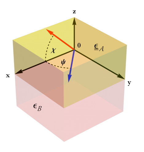
Figure 1: Schematic representation of the canonical boundary-value problem, in which material ${\cal A}$ occupies the half-space $z>0$ and material ${\cal B}$ the half-space $z<0$. The optic axis of material ${\cal A}$ lies at the angle $\chi$ to the $x$ axis in the $xz$ plane. The surface wave propagates parallel to the interface plane $z=0$ at the angle $\psi$ relative to the $x$ axis.

2.2 Half-space $z>0$

The 4$\times$4 propagation matrix $\left[\underline{\underline{P}}_{\cal A}\right]$ is given as

$$\left[\underline{\underline{P}}_{\cal A}\right]=\left[\begin{array}[]{cccc}\frac{\beta}{\gamma}&0&\frac{q^{2}\sin 2\psi}{2\omega\varepsilon_{\scriptscriptstyle 0}\gamma}&\frac{k_{o}^{2}\gamma-\nu_{c}}{\omega\varepsilon_{\scriptscriptstyle 0}\gamma}\\ \frac{\beta\tan\psi}{\gamma}&0&\frac{\nu_{s}-k_{o}^{2}\gamma}{\omega\varepsilon_{\scriptscriptstyle 0}\gamma}&\frac{-q^{2}\sin 2\psi}{2\omega\varepsilon_{\scriptscriptstyle 0}\gamma}\\ \frac{-q^{2}\sin 2\psi}{2\omega\mu_{\scriptscriptstyle 0}}&\frac{-k_{\scriptscriptstyle 0}^{2}\varepsilon^{s}_{\cal A}+\nu_{c}}{\omega\mu_{\scriptscriptstyle 0}}&0&0\\ \frac{k_{\scriptscriptstyle 0}^{2}\varepsilon^{s}_{\cal A}\varepsilon^{t}_{\cal A}-\gamma\nu_{s}}{\omega\mu_{\scriptscriptstyle 0}\gamma}&\frac{q^{2}\sin 2\psi}{2\omega\mu_{\scriptscriptstyle 0}}&-\frac{\beta\tan\psi}{\gamma}&\frac{\beta}{\gamma}\end{array}\right],$$ (6)

wherein the generally complex-valued parameters

$$\left.\begin{array}[]{l}\nu_{c}=q^{2}\cos^{2}\psi\vspace{0pt}\\ \nu_{s}=q^{2}\sin^{2}\psi\vspace{0pt}\\ \beta=q\left(\varepsilon^{s}_{\cal A}-\varepsilon^{t}_{\cal A}\right)\sin\chi\cos\chi\cos\psi\vspace{0pt}\\ \gamma=\varepsilon^{s}_{\cal A}\cos^{2}\chi+\varepsilon^{t}_{\cal A}\sin^{2}\chi\end{array}\right\}.$$ (7)

The $z$-directed components of the field phasors are

$$\left.\begin{array}[]{l}e_{z}(z)=\displaystyle{\frac{1}{\gamma}\left\{\frac{q\left[h_{x}(z)\sin\psi-h_{y}(z)\cos\psi\right]}{\omega\varepsilon_{\scriptscriptstyle 0}}\right.\vspace{4pt}}\\ \hskip 34.1433pt+\displaystyle{e_{x}(z)\left(\varepsilon^{s}_{\cal A}-\varepsilon^{t}_{\cal A}\right)\sin\chi\cos\chi\Bigg{\}}\vspace{8pt}}\\ h_{z}(z)=\displaystyle{\frac{q\left[e_{y}(z)\cos\psi-e_{x}(z)\sin\psi\right]}{\omega\mu_{\scriptscriptstyle 0}}}\end{array}\right\}\,,\qquad z>0\,.$$ (8)

2.2.1 Dyakonov surface wave

In order to deal with DV surface waves, it is necessary to first consider the case of Dyakonov surface waves for which $\left[\underline{\underline{P}}_{\cal A}\right]$ has four eigenvalues, each with algebraic multiplicity $1$ and geometric multiplicity $1$. These eigenvalues are

$$\left.\begin{array}[]{l}\alpha_{{\cal A}a}=i\sqrt{q^{2}-k_{\scriptscriptstyle 0}^{2}\varepsilon_{\cal A}^{s}}\vspace{8pt}\\ \alpha_{{\cal A}b}=-i\sqrt{q^{2}-k_{\scriptscriptstyle 0}^{2}\varepsilon_{\cal A}^{s}}\vspace{8pt}\\ \alpha_{{\cal A}c}=\displaystyle{\frac{\beta+i\sqrt{\varepsilon^{s}_{\cal A}\left[\nu_{s}\cos^{2}\chi\left(\varepsilon^{s}_{\cal A}-\varepsilon^{t}_{\cal A}\right)+q^{2}\varepsilon^{t}_{\cal A}\right]-\gamma\varepsilon^{s}_{\cal A}\varepsilon^{t}_{\cal A}k_{o}^{2}}}{\gamma}\vspace{8pt}}\\ \alpha_{{\cal A}d}=\displaystyle{\frac{\beta-i\sqrt{\varepsilon^{s}_{\cal A}\left[\nu_{s}\cos^{2}\chi\left(\varepsilon^{s}_{\cal A}-\varepsilon^{t}_{\cal A}\right)+q^{2}\varepsilon^{t}_{\cal A}\right]-\gamma\varepsilon^{s}_{\cal A}\varepsilon^{t}_{\cal A}k_{o}^{2}}}{\gamma}}\end{array}\right\}\,.$$ (9)

Only those eigenvalues which have positive imaginary parts are relevant for surface-wave propagation. Clearly, only one of $\alpha_{{\cal A}a}$ and $\alpha_{{\cal A}b}$ can have a positive imaginary part. Furthermore, it is assumed that only one of $\alpha_{{\cal A}c}$ and $\alpha_{{\cal A}d}$ can have a positive imaginary part. Therefore the two eigenvalues that are chosen [2] for our surface-wave analysis are

$$\begin{array}[]{l}\alpha_{{\cal A}1}=\left\{\begin{array}[]{lr}\alpha_{{\cal A}a}&\quad\mbox{if}\quad\mbox{Im}\left\{\alpha_{{\cal A}a}\right\}>0\vspace{0pt}\\ \alpha_{{\cal A}b}&\quad\mbox{otherwise}\end{array}\right.\end{array}$$ (10)

and

$$\begin{array}[]{l}\alpha_{{\cal A}2}=\left\{\begin{array}[]{lr}\alpha_{{\cal A}c}&\quad\mbox{if}\quad\mbox{Im}\left\{\alpha_{{\cal A}c}\right\}>0\vspace{0pt}\\ \alpha_{{\cal A}d}&\quad\mbox{otherwise}\end{array}\right.\end{array}.$$ (11)

2.2.2 Dyakonov–Voigt surface wave

In the case of DV surface-wave propagation, we have $\alpha_{{\cal A}1}=\alpha_{{\cal A}2}=\alpha_{\cal A}$. Thus, $\left[\underline{\underline{P}}_{\cal A}\right]$ has only two eigenvalues, each with algebraic multiplicity $2$ and geometric multiplicity $1$. There are are four possible values of $q$ that result in $\alpha_{{\cal A}1}=\alpha_{{\cal A}2}$, namely

$$q=\left\{\begin{array}[]{l}\displaystyle{\frac{k_{\scriptscriptstyle 0}\sqrt{\varepsilon^{s}_{\cal A}}\cos\chi\left(\cos\psi\pm i\sin\chi\sin\psi\right)}{1-\cos^{2}\chi\sin^{2}\psi}\vspace{8pt}}\\ \displaystyle{-\frac{k_{\scriptscriptstyle 0}\sqrt{\varepsilon^{s}_{\cal A}}\cos\chi\left(\cos\psi\pm i\sin\chi\sin\psi\right)}{1-\cos^{2}\chi\sin^{2}\psi}}\end{array}\right.,$$ (12)

with the correct value of $q$ for DV surface-wave propagation being the one that yields $\mbox{Im}\left\{\alpha_{{\cal A}}\right\}>0$ [2].

Explicit expressions for a corresponding eigenvector $\underline{v}_{\cal A}$ satisfying

$$\left(\left[\underline{\underline{P}}_{\cal A}\right]-\alpha_{{\cal A}}\underline{\underline{I}}\right)\mbox{ \tiny{${}^{\bullet}$} }\underline{v}_{{\cal A}}=\underline{0},$$ (13)

and a corresponding generalized eigenvector $\underline{w}_{\cal A}$ satisfying [29]

$$\left(\left[\underline{\underline{P}}_{\cal A}\right]-\alpha_{{\cal A}}\underline{\underline{I}}\right)\mbox{ \tiny{${}^{\bullet}$} }\underline{w}_{{\cal A}}=\underline{v}_{{\cal A}},$$ (14)

can be derived, but these expressions are too cumbersome to be reproduced here.

Thus, the general solution of Eq. (4)₁ representing DV surface waves that decay as $z\to+\infty$ is given as

$$\left[\underline{f}(z)\right]=\left[C_{{\cal A}1}\underline{v}_{{\cal A}}+C_{{\cal A}2}\left(iz\,\underline{v}_{{\cal A}}+\underline{w}_{{\cal A}}\right)\right]\exp\left(i\alpha_{{\cal A}}z\right)\,,\quad z>0\,.$$ (15)

The complex-valued constants $C_{{\cal A}1}$ and $C_{{\cal A}2}$ herein are fixed by applying boundary conditions at $z=0$.

2.3 Half-space $z<0$

The 4$\times$4 matrix $\left[\underline{\underline{P}}_{\cal B}\right]$ is given as [2]

$$\left[\underline{\underline{P}}_{\cal B}\right]=\left[\begin{array}[]{cccc}0&0&\displaystyle{\frac{\tau}{\omega\varepsilon_{\scriptscriptstyle 0}\varepsilon_{\cal B}}}&\displaystyle{\frac{k_{\scriptscriptstyle 0}^{2}\varepsilon_{\cal B}-\nu_{c}}{\omega\varepsilon_{\scriptscriptstyle 0}\varepsilon_{\cal B}}\vspace{8pt}}\\ 0&0&\displaystyle{\frac{\nu_{s}-k_{\scriptscriptstyle 0}^{2}\varepsilon_{\cal B}}{\omega\varepsilon_{\scriptscriptstyle 0}\varepsilon_{\cal B}}}&\displaystyle{-\frac{\tau}{\omega\varepsilon_{\scriptscriptstyle 0}\varepsilon_{\cal B}}\vspace{8pt}}\\ \displaystyle{-\frac{\tau}{\omega\mu_{\scriptscriptstyle 0}}}&\displaystyle{\frac{\nu_{c}-k_{\scriptscriptstyle 0}^{2}\varepsilon_{\cal B}}{\omega\mu_{\scriptscriptstyle 0}}}&0&0\vspace{8pt}\\ \displaystyle{\frac{k_{\scriptscriptstyle 0}^{2}\varepsilon_{\cal B}-\nu_{s}}{\omega\mu_{\scriptscriptstyle 0}}}&\displaystyle{\frac{\tau}{\omega\mu_{\scriptscriptstyle 0}}}&0&0\end{array}\right],$$ (20)

wherein the generally complex-valued parameter

$$\tau=q^{2}\cos\psi\sin\psi.$$ (22)

The $z$-directed components of the phasors are given by

$$\left.\begin{array}[]{l}e_{z}(z)=\displaystyle{\frac{q\left[h_{x}(z)\sin\psi-h_{y}(z)\cos\psi\right]}{\omega\varepsilon_{\scriptscriptstyle 0}\varepsilon_{\cal B}}\vspace{8pt}}\\ h_{z}(z)=\displaystyle{\frac{q\left[e_{y}(z)\cos\psi-e_{x}(z)\sin\psi\right]}{\omega\mu_{\scriptscriptstyle 0}}}\end{array}\right\}\,,\qquad z<0\,.$$ (23)

Matrix $\left[\underline{\underline{P}}_{\cal B}\right]$ has two distinct eigenvalues, each with algebraic multiplicity $2$ and geometric multiplicity $2$. These are denoted as $\pm\alpha_{{\cal B}}$, with

$$\alpha_{{\cal B}}=-i\sqrt{q^{2}-k_{\scriptscriptstyle 0}^{2}\varepsilon_{\cal B}}.$$ (24)

The sign of the square root in Eq. (24) must be such that $\mbox{Im}\left\{\alpha_{{\cal B}}\right\}<0$, for surface-wave propagation. A pair of independent eigenvectors of matrix $\left[\underline{\underline{P}}_{\cal B}\right]$ corresponding to the eigenvalue $\alpha_{{\cal B}}$ are

$$\left.\begin{array}[]{l}\underline{v}_{{\cal B}1}=\left[\displaystyle{1-\frac{\nu_{c}}{k_{\scriptscriptstyle 0}^{2}\varepsilon_{\cal B}}},\quad\displaystyle{-\frac{\tau}{k_{\scriptscriptstyle 0}^{2}\varepsilon_{\cal B}}},\quad 0,\quad\displaystyle{\frac{\alpha_{\cal B}}{\omega\mu_{\scriptscriptstyle 0}}}\right]^{T}\vspace{8pt}\\ \underline{v}_{{\cal B}2}=\left[\displaystyle{\frac{\tau}{k_{\scriptscriptstyle 0}^{2}\varepsilon_{\cal B}}},\quad\displaystyle{\frac{\nu_{s}}{k_{\scriptscriptstyle 0}^{2}\varepsilon_{\cal B}}-1},\quad\displaystyle{\frac{\alpha_{\cal B}}{\omega\mu_{\scriptscriptstyle 0}},\quad 0}\>\>\right]^{T}\end{array}\right\}.$$ (25)

Thus, the general solution of Eq. (4)₂ for surface waves that decay as $z\to-\infty$ is provided as

$$\left[\underline{f}(z)\right]=\left(C_{{\cal B}1}\underline{v}_{{\cal B}1}+C_{{\cal B}2}\underline{v}_{{\cal B}2}\right)\exp\left(i\alpha_{{\cal B}}z\right)\,,\qquad z<0\,,$$ (26)

with the complex-valued constants $C_{{\cal B}1}$ and $C_{{\cal B}2}$ being fixed by applying boundary conditions at $z=0$.

2.4 Application of boundary conditions

The continuity of the tangential components of the electric and magnetic field phasors across the interface plane $z=0$ imposes four conditions that are represented compactly as

$$\left[\underline{f}(0^{+})\right]=\left[\underline{f}(0^{-})\right]\,.$$ (27)

The combination of Eqs.  (15) and (26), along with Eq. (27), yields

$$\left[\underline{\underline{M}}\right]\mbox{ \tiny{${}^{\bullet}$} }\left[\>C_{{\cal A}1},\quad C_{{\cal A}2},\quad C_{{\cal B}1},\quad C_{{\cal B}2}\>\right]^{T}=\left[\>0,\quad 0,\quad 0,\quad 0\>\right]^{T},$$ (28)

wherein the 4$\times$4 characteristic matrix $\left[\underline{\underline{M}}\right]$ must be singular for surface-wave propagation [2]. The dispersion equation

$$\left|\left[\underline{\underline{M}}\right]\right|=0,$$ (29)

whose explicit representation is too cumbersome for reproduction here, can be numerically solved for $q$, by the Newton–Raphson method [30] for example .

3 Numerical studies

In order to characterize DV surface-wave propagation supported by dissipative materials, we now explore numerical solutions to the canonical boundary-value problem that satisfy the dispersion equation (29).

In the special case considered previously [21], wherein the optic axis of material ${\cal A}$ lies in the interface plane (i.e., $\chi=0^{\circ}$) and the materials ${\cal A}$ and ${\cal B}$ are nondissipative (and inactive), certain constraints on the relative permittivity parameters of materials ${\cal A}$ and ${\cal B}$ can be established. However, the general case ($0^{\circ}\leq\chi\leq 90^{\circ}$ and $\varepsilon^{s}_{\cal A}\in\mathbb{C}$, $\varepsilon^{t}_{\cal A}\in\mathbb{C}$, and $\varepsilon_{\cal B}\in\mathbb{C}$) considered here is much less amenable to analysis and such constraints are not forthcoming.

Two general observations should be noted before embarking on a presentation of numerical results:

• Only null solutions are obtained for $\chi=90^{\circ}$, which is therefore disregarded henceforth.

• No solutions are found for $\chi\in(0^{\circ},90^{\circ})$ when ${\rm Im}\left\{\varepsilon^{s}_{\cal A}\right\}=0$, ${\rm Im}\left\{\varepsilon^{t}_{\cal A}\right\}=0$, and ${\rm Im}\left\{\varepsilon_{\cal B}\right\}=0$.

Therefore, the exhibition of loss (or gain) by at least one of the two partnering materials is a prerequisite for DV surface-wave propagation when the optic axis of material ${\cal A}$ does not lie wholly in the interface plane.

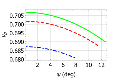
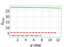
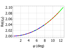
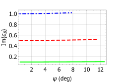
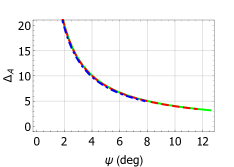
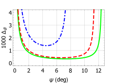
Figure 2: Real and imaginary parts of relative permittivity $\varepsilon_{\cal B}$, normalized phase speed $v_{\text{p}}$, normalized propagation length $\Delta_{\text{prop}}$, normalized penetration depths $\Delta_{\cal A}$ and $\Delta_{\cal B}$ plotted versus propagation angle $\psi$, for $\chi=0^{\circ}$, $\varepsilon^{s}_{\cal A}=2+\delta i$, and $\varepsilon^{t}_{\cal A}=6.2+2\delta i$, when $\delta=0.1$ (green solid curves), $\delta=0.5$ (red dashed curves), and $\delta=1$ (blue dot-dashed curves).

3.1 $\chi=0^{\circ}$

Let us begin our presentation with the case $\chi=0^{\circ}$. We fixed $\varepsilon^{s}_{\cal A}=2+\delta i$ and $\varepsilon^{t}_{\cal A}=6.2+2\delta i$ for calculations. The corresponding real and imaginary parts of $\varepsilon_{\cal B}$ that satisfies the dispersion equation (29) are plotted versus the propagation angle $\psi$ in Fig. 2 for $\delta\in\left\{0.1,0.5,1\right\}$.

Solutions only exist for relatively small ranges of $\psi$, and these $\psi$-ranges shrink as $\delta$ increases. Thus, solutions exist for $0^{\circ}<\psi<12.5^{\circ}$ when $\delta=0.1$, but only for $0^{\circ}<\psi<6.8^{\circ}$ when $\delta=1$. The real part of $\varepsilon_{\cal B}$ increases monotonically as $\psi$ increases, taking the value of $\varepsilon^{s}_{\cal A}$ at $\psi=0^{\circ}$; and $\mbox{Re}\left\{\varepsilon_{\cal B}\right\}$ is very nearly independent of $\delta$. On the other hand, the imaginary part of $\varepsilon_{B}$ is very nearly independent of $\psi$, but $\mbox{Im}\left\{\varepsilon_{\cal B}\right\}$ increases substantially as $\delta$ increases with $\mbox{Im}\left\{\varepsilon_{\cal B}\right\}\approx\mbox{Im}\left\{\varepsilon^{s}_{\cal A}\right\}$.

Plots of the normalized phase speed

$$v_{\text{p}}=\frac{k_{\scriptscriptstyle 0}}{\mbox{Re}\left\{q\right\}},$$ (30)

and the normalized propagation length

$$\Delta_{\text{prop}}=\frac{k_{\scriptscriptstyle 0}}{\mbox{Im}\left\{q\right\}}$$ (31)

versus $\psi$ are also provided in Fig. 2. Both $v_{\text{p}}$ and $\Delta_{\text{prop}}$ are dimensionless quantities. The phase speed decreases monotonically as $\psi$ increases, for all values of $\delta$, with $v_{\text{p}}$ being greatest for the smallest value of $\delta$. On the other hand, the propagation length is almost independent of $\psi$, with $\Delta_{\text{prop}}$ being greatest for the smallest value of $\delta$.

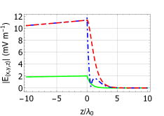
Figure 3: $|\underline{E}(z\hat{\underline{u}}_{z})\mbox{ \tiny{${}^{\bullet}$} }\underline{n}|$, $|\underline{H}(z\hat{\underline{u}}_{z})\mbox{ \tiny{${}^{\bullet}$} }\underline{n}|$, and $\underline{P}(z\hat{\underline{u}}_{z})\mbox{ \tiny{${}^{\bullet}$} }\underline{n}$ plotted versus $z/\lambda_{\scriptscriptstyle 0}$, for $\varepsilon^{s}_{\cal A}=2+0.5i$, $\varepsilon^{t}_{\cal A}=6.2+i$, $\varepsilon_{\cal B}=2.062+0.516i$, $\chi=0^{\circ}$, and $\psi=10^{\circ}$, with $C_{\mathcal{B}1}=1$ V m^-1, for $\underline{n}=\hat{\underline{u}}_{x}$ (green solid curves), $\underline{n}=\hat{\underline{u}}_{y}$ (red dashed curves), and $\underline{n}=\hat{\underline{u}}_{z}$ (blue dot-dashed curves).

Also presented in Fig. 2 are the corresponding plots of

$$\left.\begin{array}[]{l}\Delta_{\cal A}=\displaystyle{\frac{k_{\scriptscriptstyle 0}}{\mbox{Im}\left\{\alpha_{\cal A}\right\}}\vspace{8pt}}\\ \Delta_{\cal B}=\displaystyle{-\frac{k_{\scriptscriptstyle 0}}{\mbox{Im}\left\{\alpha_{\cal B}\right\}}}\end{array}\right\},$$ (32)

which represent the normalized penetration depths [2] in the partnering materials ${\cal A}$ and ${\cal B}$, respectively. Both $\Delta_{\cal A}$ and $\Delta_{\cal B}$ are dimensionless quantities. Let us note that $\Delta_{\cal A}$ is very nearly independent of $\delta$; furthermore, $\Delta_{\cal A}$ increases monotonically as $\psi$ decreases, becoming unbounded as $\psi$ approaches $0^{\circ}$. In contrast, for each value of $\delta$, $\Delta_{\cal B}$ has a minimum, with the minimum value of $\Delta_{\cal B}$ being larger for larger $\delta$. Also, $\Delta_{\cal B}$ becomes unbounded as $\psi$ approaches either of its two extreme values.

Further light is shed by the spatial profiles of the magnitudes of the Cartesian components of the electric and magnetic field phasors in Fig. 3 for $\delta=0.5$ and $\psi=10^{\circ}$. The dispersion equation (29) then yields $\varepsilon_{\cal B}=2.062+0.516i$. The magnitudes of the components of the electric and magnetic field phasors decay as the distance $|{z}|$ from the interface plane increases. The rate of decay is much faster in material ${\cal A}$ than in material ${\cal B}$. Furthermore, beyond a short distance (approximately 1.5 $\lambda_{\scriptscriptstyle 0}$) from the interface plane, the decay in material ${\cal A}$ appears to exponential, from which it may be inferred that the linear term in Eq. (15) is dominated by the exponentially decaying terms.

The localization of the DV surface waves is also revealed by profiles of the Cartesian components of the time-averaged Poynting vector

$$\underline{P}(\underline{r})=\frac{1}{2}\mbox{Re}\left\{\,\underline{E}(\underline{r})\times\underline{H}^{*}(\underline{r})\,\right\}$$ (33)

presented in Fig. 3. These profiles show that energy flow is concentrated in directions parallel to the interface plane $z=0$.

3.2 $\chi\in(0^{\circ},90^{\circ})$

Next we turn to $\chi\in(0^{\circ},90^{\circ})$. As in Sec. 3.3.1, we fix $\varepsilon^{s}_{\cal A}=2+\delta i$ and $\varepsilon^{t}_{\cal A}=6.2+2\delta i$ but vary $\delta\in\left\{0.1,0.5,1\right\}$.

3.2.1 $\chi=45^{\circ}$

For the sake of illustration, we focus our attention on $\chi=45^{\circ}$, which is equidistant from both extremities of the range $0^{\circ}<\chi<90^{\circ}$. Zero, one, or two solutions of the dispersion equation (29) can be found for each value of $\delta$, depending on the value of $\psi$. These solutions can be organized into three branches with $\psi$ as a variable. Whereas the first branch spans only large values of $\psi$, as becomes clear from Fig. 4, Figs. 5 and 6 show that the second and the third branches span only small values of $\psi$, respectively. The $\psi$-range in which at least one solution exists is of quite small extent ($\sim 2^{\circ}$) when $\delta=0.1$, but that extent widens to $\sim 9^{\circ}$ when $\delta=1$.

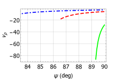
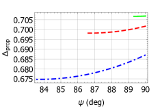
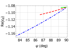
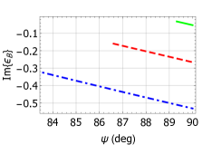
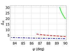
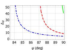
Figure 4: As Fig. 2 but for the first solution branch when $\chi=45^{\circ}$.

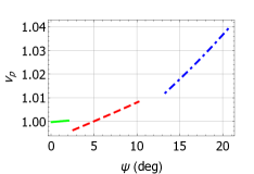
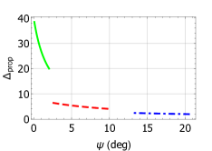
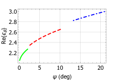
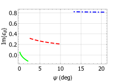
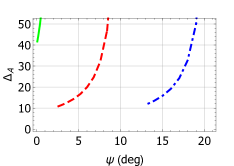
Figure 5: As Fig. 2 but for the second solution branch when $\chi=45^{\circ}$.

For the first solution branch, as illustrated in Fig. 4, the dispersion equation (29) yields values of $\varepsilon_{\cal B}$ for $\psi$ close to $90^{\circ}$. As $\mbox{Re}\left\{\varepsilon_{\cal B}\right\}<0$ and $\mbox{Im}\left\{\varepsilon_{\cal B}\right\}<0$ for all values of $\delta$, the partnering material ${\cal B}$ must be an active plasmonic material [31, 32]. The magnitudes of both $\mbox{Re}\left\{\varepsilon_{\cal B}\right\}$ and $\mbox{Im}\left\{\varepsilon_{\cal B}\right\}$ are larger for larger values of $\delta$. The magnitudes of the phase speeds in Fig. 4 are much larger than the corresponding phase speeds in Fig. 2. Also, $v_{\text{p}}<0$ in Fig. 4 for all values of $\delta$, whereas $v_{\text{p}}>0$ for all values of $\delta$ in Fig. 2. Thus, the DV surface waves on the first solution branch propagate with negative phase velocity; this phenomenon has recently been reported for surface waves supported by hyperbolic materials [33]. At a fixed value of $\psi$, the propagation length $\Delta_{\text{prop}}$, and the penetration depths $\Delta_{\cal A}$ and $\Delta_{\cal B}$, in Fig. 4 are all larger when $\delta$ is smaller. In addition, $\Delta_{\cal B}$ becomes unbounded as $\psi$ approaches its lowest value.

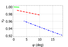
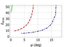
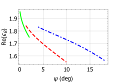
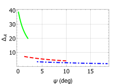
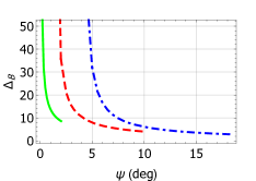
Figure 6: As Fig. 2 but for the third solution branch when $\chi=45^{\circ}$.

For the second solution branch, $\mbox{Re}\left\{\varepsilon_{\cal B}\right\}>0$ for all values of $\delta$ in Fig. 5. Also $\mbox{Im}\left\{\varepsilon_{\cal B}\right\}>0$ except for a small range of $\psi$ values when $\delta=0.1$. Thus, for most values of $\delta$ and $\psi$, the partnering material ${\cal B}$ is a dissipative dielectric material. The magnitudes of both $\mbox{Re}\left\{\varepsilon_{\cal B}\right\}$ and $\mbox{Im}\left\{\varepsilon_{\cal B}\right\}$ are larger for larger values of $\delta$. The phase speeds in Fig. 5 are much smaller in magnitude than those in Fig. 4. Also, all the phase speeds in Fig. 5 are positive, unlike those in Fig. 4. For all values of $\delta$ in Fig. 5, the penetration depth $\Delta_{\cal A}$ becomes unbounded as $\psi$ approaches its maximum value, whereas the penetration depth $\Delta_{\cal B}$ becomes unbounded as $\psi$ approaches its minimum value.

For the third solution branch, $\mbox{Re}\left\{\varepsilon_{\cal B}\right\}>0$ for all values of $\delta$ in Fig. 6; however, $\mbox{Im}\left\{\varepsilon_{\cal B}\right\}>0$ for small values of $\psi$ but $\mbox{Im}\left\{\varepsilon_{\cal B}\right\}<0$ for large values of $\psi$. Thus, the partnering material ${\cal B}$ is dissipative dielectric for small values of $\psi$ and an active dielectric for large values of $\psi$. The phase speeds in Fig. 6 are positive, like those in Fig. 5. For all values of $\delta$, the propagation length $\Delta_{\text{prop}}$ in Fig. 6 becomes unbounded as $\psi$ approaches its maximum value, while the penetration depth $\Delta_{\cal B}$ becomes unbounded as $\psi$ approaches its minimum value.

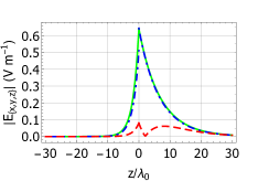
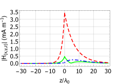
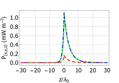
Figure 7: As Fig. 3 but for $\delta=0.5$, $\chi=45^{\circ}$, and $\psi=8^{\circ}$, so that $\varepsilon_{\mathcal{B}}=2.588+0.266i$ for DV surface-wave propagation.

In Fig. 7, the spatial profiles of the magnitudes of the Cartesian components of $\underline{E}(z\hat{\underline{u}}_{z})$ and $\underline{H}(z\hat{\underline{u}}_{z})$, as well as the Cartesian components of $\underline{P}(z\hat{\underline{u}}_{z})$, are presented for a solution lying on the branch depicted in Fig. 5 for $\delta=0.5$. The relative rate of decay of the fields in material ${\cal B}$ as $|z|/\lambda_{\scriptscriptstyle 0}$ increases is much faster in Fig. 7 than in Fig. 3. Also, there is relatively more energy flow concentrated in directions normal to the interface plane $z=0$ in Fig. 7 than in Fig. 3.

3.2.2 $\chi=85^{\circ}$

As DV surface-wave propagation is not possible for $\psi=90^{\circ}$, finally we explore the case where $\chi=85^{\circ}$. Unlike the three solution branches shown for $\chi=45^{\circ}$ in Sec. 3.3.2.1, only one solution branch exists for $\chi=85^{\circ}$, regardless of the value of $\delta>0$. In Fig. 8, $\mbox{Re}\left\{\varepsilon_{\cal B}\right\}>0$ and $\mbox{Im}\left\{\varepsilon_{\cal B}\right\}>0$ for all values of $\delta$. The magnitudes of both the real and imaginary parts of $\varepsilon_{\cal B}$ are tiny compared to those for $\chi=0^{\circ}$ (Fig. 2) and $\chi=45^{\circ}$ (Figs. 4–6). Additionally, $\mbox{Im}\left\{\varepsilon_{\cal B}\right\}$ is approximately one order of magnitude smaller than $\mbox{Re}\left\{\varepsilon_{\cal B}\right\}$. Thus, material ${\cal B}$ is a dissipative dielectric material. Also, $\mbox{Re}\left\{\varepsilon_{\cal B}\right\}$ increases, but $\mbox{Im}\left\{\varepsilon_{\cal B}\right\}$ decreases, as $\psi$ increases.

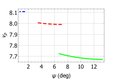
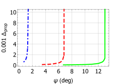
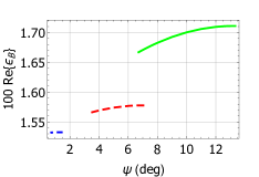
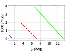
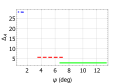
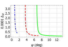
Figure 8: As Fig. 2 but when $\chi=85^{\circ}$.

The phase speeds presented in Fig. 8 are positive and relatively large, with $v_{\text{p}}$ being larger when $\delta$ is larger. The propagation lengths $\Delta_{\text{prop}}$ and the penetration depths $\Delta_{\cal B}$ presented in Fig. 8 are generally tiny, but $\Delta_{\text{prop}}$ rapidly becomes unbounded as $\psi$ approaches its maximum value and $\Delta_{\cal B}$ rapidly becomes unbounded as $\psi$ approaches its minimum value.

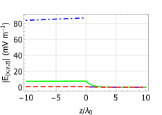
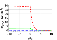
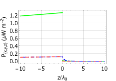
Figure 9: As Fig. 3 but for $\delta=0.5$, $\chi=85^{\circ}$, and $\psi=5^{\circ}$, so that $\varepsilon_{\mathcal{B}}=0.016+0.001i$ for DV surface-wave propagation.

Spatial profiles of the magnitudes of the Cartesian components of $\underline{E}(z\hat{\underline{u}}_{z})$ and $\underline{H}(z\hat{\underline{u}}_{z})$, as well as spatial profiles of the Cartesian components of $\underline{P}(z\hat{\underline{u}}_{z})$, are presented in Fig. 9 for $\delta=0.5$ and $\psi=5^{\circ}$, so that $\varepsilon_{\cal B}=0.016+0.001i$. Parethetically, such values of relative permittivity that are close to zero can be realized using metamaterial technologies [34, 35]. The plots in Fig. 9 are qualitatively similar to those in Fig. 3, the most obvious difference being that there is relatively more energy flow concentrated in directions normal to the interface plane $z=0$, especially in material ${\cal B}$, than in Fig. 3.

4 Closing remarks

Dyakonov–Voigt surface waves guided by the planar interface of a uniaxial dielectric material ${\cal A}$ and an isotropic dielectric material ${\cal B}$ were numerically investigated by formulating and solving the corresponding canonical boundary-value problem. The degree of dissipation and the inclination angle $\chi$ of the optic axis of material ${\cal A}$ were found to profoundly influence the phase speeds, propagation lengths, and penetration depths of the DV surface waves. Notably, for mid-range values of $\chi$, DV surface waves with negative phase velocity were found when material ${\cal A}$ is dissipative and material ${\cal B}$ is active. For fixed values of $\varepsilon^{s}_{\cal A}$ and $\varepsilon^{t}_{\cal A}$ in the upper-half-complex plane, DV surface-wave propagation is only possible for large values of $\chi$ when $|\varepsilon_{\cal B}|$ is very small.

In the presented numerical studies, the relative permittivity parameters $\varepsilon^{s}_{\cal A}$ and $\varepsilon^{t}_{\cal A}$ were fixed (in the upper-half-complex plane) and the dispersion equation (29) solved to find $\varepsilon_{\cal B}$. We also conducted numerical studies (not presented here) wherein $\varepsilon^{t}_{\cal A}$ and $\varepsilon_{\cal B}$ were fixed (in the upper-half-complex plane) and the dispersion equation (29) was solved to find $\varepsilon^{s}_{\cal A}$. Analogously to the presented studies, these other studies revealed that the imaginary parts of $\varepsilon^{t}_{\cal A}$ and $\varepsilon_{\cal B}$ have a profound influence on the characteristics of the DV surface waves. Furthermore, in this case solutions to the dispersion equation (29) were found for which $\mbox{Im}\left\{\varepsilon^{s}_{\cal A}\right\}<0$ and $\mbox{Im}\left\{\varepsilon^{t}_{\cal A}\right\}>0$, indicating that material ${\cal A}$ is simultaneously both dissipative and active depending upon propagation direction [36, 37].

Our numerical studies do not reveal physical mechanisms. In the case of Dyakonov surface waves, it is well established that dissipative partnering materials support wider angular existence domains than do nondissipative partnering materials [17, 18]. However, an analogous observation is not forthcoming for Dyakonov–Voigt surface waves.

Finally, the numerical studies presented herein were based on the corresponding canonical boundary-value problem. The canonical boundary-value problem represents an idealization: the finite thicknesses of the partnering materials and the means by which the DV surface waves are excited are not taken into account. Nevertheless, such studies of the canonical boundary-value problem deliver useful insights into the essential physics of surface-wave propagation, and represent an essential step towards the elucidation of DV surface waves in experimental scenarios.

Acknowledgments. This work was supported in part by EPSRC (grant number EP/S00033X/1) and US NSF (grant number DMS-1619901). AL thanks the Charles Godfrey Binder Endowment at the Pennsylvania State University and the Otto Mønsted Foundation for partial support of his research endeavors.

References

- [1] A.D. Boardman (Ed.), Electromagnetic Surface Modes (Wiley, 1982).
- [2] J.A. Polo Jr., T.G. Mackay, and A. Lakhtakia, Electromagnetic Surface Waves: A Modern Perspective (Elsevier, 2013).
- [3] O. Takayama, A.A. Bogdanov, and A.V. Lavrinenko, “Photonic surface waves on metamaterial interfaces,” J. Phys.: Cond. Mat. 29, 463001 (2017).
- [4] H.C. Chen, Theory of Electromagnetic Waves (McGraw–Hill, 1983).
- [5] F.N. Marchevskiĭ, V.L. Strizhevskiĭ, and S.V. Strizhevskiĭ, “Singular electromagnetic waves in bounded anisotropic media,” Sov. Phys. Solid State 26, 911–912 (1984).
- [6] M.I. D’yakonov, “New type of electromagnetic wave propagating at an interface,” Sov. Phys. JETP 67, 714–716 (1988).
- [7] O. Takayama, L. Crasovan, D. Artigas, and L. Torner, “Observation of Dyakonov surface waves,” Phys. Rev. Lett. 102, 043903 (2009).
- [8] D.P. Pulsifer, M. Faryad, and A. Lakhtakia, “Observation of the Dyakonov–Tamm wave,” Phys. Rev. Lett. 111, 243902 (2013).
- [9] O. Takayama, D. Artigas, and L. Torner, “Lossless directional guiding of light in dielectric nanosheets using Dyakonov surface waves,” Nature Nanotech. 9, 419–424 (2014).
- [10] J.M. Pitarke, V.M. Silkin, E.V. Chulkov, and P.M. Echenique, “Theory of surface plasmon and surface-plasmon polaritons,” Rep. Prog. Phys. 70, 1–87 (2007).
- [11] J. Homola (Ed.), Surface Plasmon Resonance Based Sensors (Springer, 2006).
- [12] O. Takayama, L.-C. Crasovan, S.K. Johansen, D. Mihalache, D. Artigas, and L. Torner, “Dyakonov surface waves: A review,” Electromagnetics 28, 126–145 (2008).
- [13] D.B. Walker, E.N. Glytsis, and T.K. Gaylord, “Surface mode at isotropic-uniaxial and isotropic-biaxial interfaces,” J. Opt. Soc. Am. A 15, 248–260 (1998).
- [14] V.I. Alshits and V.N. Lyubimov, “Dispersionless surface polaritions in the vicinity of different sections of optically uniaxial crystals,” Phys. Solid State 44, 386–390 (2002).
- [15] J.A. Polo Jr., S. Nelatury, and A. Lakhtakia, “Surface electromagnetic wave at a tilted uniaxial bicrystalline interface,” Electromagnetics 26, 629–642 (2006).
- [16] S.R. Nelatury, J.A. Polo Jr., and A. Lakhtakia, “On widening the angular existence domain for Dyakonov surface waves using the Pockels effect,” Microwave Opt. Technol. Lett. 50, 2360–2362 (2008).
- [17] J.A. Sorni, M. Naserpour, C.J. Zapata-Rodríguez, and J.J. Miret, “Dyakonov surface waves in lossy metamaterials,” Opt. Commun. 355, 251–255 (2015).
- [18] T.G. Mackay and A. Lakhtakia, “Temperature-mediated transition from Dyakonov surface waves to surface-plasmon-polariton waves,” IEEE Photonics J. 8, 4802813 (2016).
- [19] L.-C. Crasovan, D. Artigas, D. Mihalache, and L. Torner, “Optical Dyakonov surface waves at magnetic interfaces,” Opt. Lett. 30, 3075–3077 (2005).
- [20] L.-C. Crasovan, O. Takayama, D. Artigas, S. K. Johansen, D. Mihalache, and L. Torner, “Enhanced localization of Dyakonov-like surface waves in left-handed materials,” Phys. Rev. B 74, 155120 (2006).
- [21] T.G. Mackay, C. Zhou, and A. Lakhtakia, “Dyakonov–Voigt surface waves,” Proc. R. Soc. A 475, 20190317 (2019).
- [22] W. Voigt, “On the behaviour of pleochroitic crystals along directions in the neighbourhood of an optic axis,” Phil. Mag. 4, 90–97 (1902).
- [23] S. Pancharatnam, “The propagation of light in absorbing biaxial crystals — I. Theoretical,” Proc. Ind. Acad. Sci. A 42, 86–109 (1955).
- [24] B.N. Grechushnikov and A.F. Konstantinova, “Crystal optics of absorbing and gyrotropic media,” Comput. Math. Applic. 16, 637–655 (1988).
- [25] G.S. Ranganath, “Optics of absorbing anisotropic media,” Curr. Sci. (India) 67, 231–237 (1994).
- [26] J. Gerardin and A. Lakhtakia, “Conditions for Voigt wave propagation in linear, homogeneous, dielectric mediums,” Optik 112, 493–495 (2001).
- [27] T.G. Mackay and A. Lakhtakia, Electromagnetic Anisotropy and Bianisotropy: A Field Guide, 2nd Edition (World Scientific, 2019).
- [28] D.W. Berreman, “Optics in stratified and anisotropic media: 44-matrix formulation,” J. Opt. Soc. Am. 62, 502–510 (1972).
- [29] W.E. Boyce and R.C. DiPrima, Elementary Differential Equations and Boundary Value Problems, 9th Edition (Wiley, 2010).
- [30] Y. Jaluria, Computer Methods for Engineering (Taylor & Francis, 1996).
- [31] K.F. MacDonald and N.I. Zheludev, “Active plasmonics: current status,” Laser Photonics Rev. 4, 562–567 (2010).
- [32] N. Jiang, X. Zhou, and J. Wang, “Active plasmonics: principles, structures, and applications,” Chem. Rev. 118, 3054–3099 (2018).
- [33] T.G. Mackay and A Lakhtakia, “Surface waves with negative phase velocity supported by temperature-dependent hyperbolic materials,” J. Opt. (UK) 21, 085103 (2019).
- [34] A.V. Goncharenko and K.-R. Chen, “Strategy for designing epsilon-near-zero nanostructured metamaterials over a frequency range,” J. Nanophotonics 4, 041530 (2010).
- [35] X. Niu, X. Hu, S. Chu, and Q. Gong, “Epsilon-near-zero photonics: a new platform for integrated devices,” Adv. Optical Mater. 6, 1701292 (2018).
- [36] T.G. Mackay and A. Lakhtakia, “Dynamically controllable anisotropic metamaterials with simultaneous attenuation and amplification,” Phys. Rev. A 92, 053847 (2015).
- [37] T.G. Mackay and A. Lakhtakia, “Simultaneous existence of amplified and attenuated Dyakonov surface waves,” Opt. Commun. 427, 175–179 (2018).