Polaritonic Contribution to the Casimir Energy between two Graphene Layers

Abstract

We study the role of surface polaritons in the zero-temperature Casimir effect between two graphene layers that are described by the Dirac model. A parametric approach allows us to accurately calculate the dispersion relations of the relevant modes and to evaluate their contribution to the total Casimir energy. The resulting force features a change of sign from attractive to repulsive as the distance between the layers increases. Contrary to similar calculations that have been performed for metallic plates, our asymptotic analysis demonstrates that at small separations the polaritonic contribution becomes negligible relative to the total energy.

I Introduction

As technology progresses further towards miniaturization, effects that are usually imperceptible at large scales start to become important. Prominent examples are dispersion forces and in particular the Casimir effect which, in its simplest form, describes an attractive interaction between two electrically neutral nonmagnetic macroscopic objects placed in vacuum at zero temperature. In the approach originally followed by Casimir in 1948 casimir48 , the force was derived by summing the zero-point energies associated with the electromagnetic modes of the system. In the case of an empty cavity formed by two parallel material interfaces, the Casimir energy is given by

$$E=\sum_{\sigma,n}\sum_{\textbf{k}}\left[\frac{\hbar}{2}\omega_{n}^{\sigma}(\mathbf{k},L)\right]_{L\rightarrow\infty}^{L},$$ (1)

where $\hbar$ is the reduced Planck constant, $\sigma=\textrm{TE},\textrm{TM}$ indicates the field polarization and $\textbf{k}=(k_{x},k_{y})$ is the component of the wavevector parallel to the interfaces. The bracket notation describes the regularization procedure introduced by Casimir to extract a finite result and implies the difference between the sum evaluated at a finite separation $L$ of the material interfaces and the same sum calculated in the limit $L\to\infty$. Physically this amounts to setting the zero of the energy to correspond to a configuration where no interaction between the objects occurs.

While in the summation every mode is treated equally, this does not mean that their relative contributions to the final result are equal, too. In fact, in earlier calculations it was pointed out that, for the Casimir effect, surface polariton modes play a special role van-kampen68 ; henkel04 ; intravaia05 ; barton05 ; bordag06 ; intravaia07 ; haakh16 . These surface polaritons are mixed light-matter excitations that exist at the interface of two media and are usually associated with electromagnetic fields which decay exponentially away from the surface economou69 ; joulain05 ; pitarke07 ; maier07 . Over the last decade, these solutions of the Maxwell equations have attracted considerable interest due to their unique properties and the possibilities they offer to nano-photonics and (quantum) optical technologies nie97 ; ebbesen98 ; maier07 ; torma15 . Specifically, in the case of two metallic plates it has been shown that the surface plasmon polaritons dominate the Casimir interaction at short distances and strongly affect the force at large distances. This suggests to control the Casimir effect by manipulating the surface polaritons’ properties via structuring the surface Intravaia12a ; intravaia13 .

Other methods to tailor the interaction usually rely on the optical properties of the materials comprising the objects. For instance, in recent studies graphene has emerged as an interesting candidate and, due to its exotic properties, is being considered both in theoretical and experimental research fialkovsky11 ; banishev13 ; Biehs14 ; klimchitskaya15 ; klimchitskaya15a ; bordag16 ; Henkel18 ; Klimchitskaya18a . In fact, this research is also relevant in connection to the role played by dispersion forces in the context of so-called van der Waals materials Geim13 ; Gobre13 ; Novoselov16 ; Ambrosetti16 ; Woods16 . For such investigations, an adequate theoretical description of graphene’s optical properties is important in order to predict the right magnitudes of the Casimir force at the relevant length scales klimchitskaya15 . One of the most successful corresponding material model is the so-called Dirac model, which describes the collective motion of the electrons in graphene in terms of a (2+1) Dirac field mccann12 .

In this manuscript, we merge the previous perspectives and analyze the role of the surface polaritons for the Casimir effect between two graphene layers that are described by the Dirac model. In our approach, we consider the case where graphene might feature a small gap $\Delta$ in its band structure klimchitskaya15 ; Werra16 , due to, for example, strain or impurities Zhou07 ; Giovannetti07 ; Chen14 ; Jung15 . In Sec. II we start by analyzing the behavior of the scattering coefficients for a single graphene layer described within the Dirac model. We then calculate the total Casimir energy at zero temperature and determine its behavior for short and large separations between the layers (Sec. III) . Based on this analysis, we proceed in Sec. IV to calculating the dispersion relation of the polaritonic modes and, in Sec. V, their contribution to the Casimir energy. Specifically, we contrast the asymptotic behavior of the polaritonic contribution to that of the total energy in order to highlight the analogies and the differences with respect to the result obtained for ordinary metals intravaia07 . In Section VI, we discuss our findings.

II Dirac Model for Graphene

The Dirac model describes the electronic excitations in graphene as fermions moving in (2+1) spacetime dimensions at the Fermi velocity $v=v_{\mathrm{F}}/c\approx 1/300$, where $c$ is the speed of light in vacuum. This effective description is valid up to an energy $E_{\rm Max}$ of a few eV. Therefore, this sets a frequency limit $\omega_{\rm Max}$ of hundreds of terahertz beyond which the reliability of the results for graphene’s optical response obtained within this approach becomes questionable. Pristine graphene corresponds to massless fermions mccann12 . However, previous work has shown that graphene’s band structure may feature a band gap $\Delta\approx 5-50\text{meV}$ Zhou07 ; Giovannetti07 ; Chen14 ; Jung15 , which can be modeled as an effective mass in the (effective) Dirac equation. This introduces an additional scale into our system which, in terms of a Compton-like wavelength, is given by $\lambda_{\Delta}=\hbar c/2\Delta$. For the values of the gap mentioned above we have that $\lambda_{\Delta}\approx 2-20\,\mu$m.

Within this description, the scattering (reflection and transmission) coefficients for a single graphene layer can be obtained by solving a spinor loop diagram in the aforementioned (2+1) dimensions and subsequently coupling the emerging polarization tensor to the electromagnetic field fialkovsky11 ; chaichian12 . Following this approach, the reflection coefficients can be written as

$$r_{\mathrm{TM}}(\omega,k)=\frac{\kappa\underline{\Pi}_{00}}{\kappa\underline{\Pi}_{00}+2k^{2}},$$ (2a)

$$r_{\mathrm{TE}}(\omega,k)=\frac{k^{2}\underline{\Pi}_{\mathrm{tr}}-\kappa^{2}\underline{\Pi}_{00}}{k^{2}\left(\underline{\Pi}_{\mathrm{tr}}+2\kappa\right)-\kappa^{2}\underline{\Pi}_{00}},$$ (2b)

where $k=|\mathbf{k}|=\sqrt{k_{x}^{2}+k_{y}^{2}}$ and $\kappa=\sqrt{k^{2}-\omega^{2}/c^{2}}=-\mathrm{i}k_{z}$ is connected to the wavevector component perpendicular to the plane. The definition of the square root is chosen so that $\mathrm{Im}[\kappa]<0$ and $\mathrm{Re}[\kappa]\geq 0$: $\kappa$ is real for evanescent waves and imaginary in the propagating sector. $\underline{\Pi}$ is the polarization tensor, where $\underline{\Pi}_{00}$ denotes its “00” entry (the index “0” corresponding to the time dimension) and $\underline{\Pi}_{\mathrm{tr}}$ denotes the polarization tensor’s trace (over the temporal index “0” and the spatial indices “1” and “2”) fialkovsky11 . For arbitrary temperature, nonzero chemical potential and a nonzero band gap, the polarization tensor and its components feature rather complicated expressions fialkovsky11 ; chaichian12 . The previous equations for the reflection coefficients take into account the nonlocal interaction between the electromagnetic field and the electrons in graphene and, in the appropriate limits, reduce to the expressions in the so-called optical approximation Falkovsky07 ; Falkovsky08 . For simplicity, we restrict ourselves to the case of zero temperature ($T=0$) and undoped sheets, corresponding to a vanishing chemical potential. It is also convenient to define the dimensionless quantities $\lambda=L/\lambda_{\Delta}$, $K=k\lambda_{\Delta}$, $\Omega=\omega\lambda_{\Delta}/c$ and $\mu=\kappa\lambda_{\Delta}=\sqrt{K^{2}-\Omega^{2}}$. Within this notation, the entries of the polarization tensor take on a more compact form and we can write

$$\underline{\Pi}_{00}(\Omega,K,\Delta)=2\frac{\alpha}{\lambda_{\Delta}}\frac{K^{2}}{p^{2}}\psi\left(p\right),$$ (3a)

$$\underline{\Pi}_{\mathrm{tr}}(\Omega,K,\Delta)=2\frac{\alpha}{\lambda_{\Delta}}\frac{\mu^{2}-p^{2}}{p^{2}}\psi\left(p\right),$$ (3b)

where $\alpha$ is the fine-structure constant, $p=\sqrt{\Omega^{2}-v^{2}K^{2}}$ and $\psi(p)=\left(p+1/p\right)\text{arctanh}(p)-1$ bordag15 . The function $\psi(p)$ is positive for $0<p<1$. For $p\to 0$, it behaves as $\psi(p)\approx 4p^{2}/3$ and it diverges for $p\to 1$. The value $p=1$ corresponds to an effective pair-creation threshold and physically corresponds to the case where the energy of the (2+1) Dirac field equates the gap (i.e. the effective mass). In the $\Omega$-$K$-plane the pair-creation threshold regime is represented by the curve $\Omega_{\mathrm{pc}}(K)=\sqrt{1+v^{2}K^{2}}$ (see Fig. 2). For $p>1$ the function $\psi(p)$ as well as the reflection coefficients become complex quantities, indicating the conversion of some of the energy in electron-hole pair excitations. The limit $p\gg 1$ is equivalent to the case $\Delta\to 0$ and gives $\psi(p)\to\mathrm{i}p\pi/2$.

For zero temperature and undoped sheets the reflection coefficients take the form

$$r_{\mathrm{TM}}(\Omega,K)=\frac{\alpha\mu\psi(p)}{\alpha\mu\psi(p)+p^{2}},r_{\mathrm{TE}}(\Omega,K)=-\frac{\alpha\psi(p)}{\alpha\psi(p)-\mu}.$$ (4)

Here, their dependence on $\Omega$ and $K$ is implicitly captured via the parameters $\mu$ and $p$. As expected on physical grounds, the above expressions show that for our system the scattering of the electromagnetic radiation is controlled in strength via the fine-structure constant $\alpha$ and, therefore, is generally weaker than for ordinary materials. The above reflection coefficients do not fulfill the ultraviolet transparency condition and do not vanish in the limit $\Omega\to\infty$, where $r\sim\alpha$. However, as discussed above, it is well-known that in this limit the Dirac model becomes unreliable, a characteristic feature which has to be taken into account when interpreting corresponding calculations.

III Casimir Energy of Graphene

Before we focus on the contribution of the polaritonic modes it is useful to analyze the behavior of the total Casimir energy per area. It is given by the Lifshitz formula lifshitz56 which for our system reads

$$E(L)/A=\hbar\int\limits_{0}^{\infty}\frac{\mathrm{d}\xi}{2\pi}\int\frac{\mathrm{d}^{2}\mathbf{k}}{(2\pi)^{2}}\sum_{\sigma}\ln\left[1-r^{2}_{\sigma}(i\xi,k)e^{-2\kappa L}\right],$$ (5)

where $r_{\sigma}(i\xi,k)$ are the reflection coefficients evaluated along the positive imaginary frequency axis in the complex $\omega$-plane and $A$ denotes the area of the layers. For our purposes and in analogy to the procedure followed in previous works genet03 ; intravaia07 , it is convenient to introduce the correction factor

$$\eta=E(L)/E_{\rm perf}(L),\quad E_{\rm perf}(L)=-\frac{\hbar c\pi^{2}}{720}\frac{A}{L^{3}},$$ (6)

which describes the impact of the material properties with respect to the expression for the Casimir energy between two perfectly reflecting surfaces, $E_{\rm perf}(L)$. Since the perfect electric conductor limit represents an upper bound for the Casimir effect between two identical material layers, $\eta\leq 1$ indicates that realistic material properties lead to an interaction with reduced strength. In general, the correction factor depends on the system’s parameters and, at short layer separations and for ordinary materials, it goes to zero $\propto L$, describing the transition from the retarded ($\propto L^{-3}$) to the nonretarded (van der Waals) limit of the Casimir energy ($\propto L^{-2}$) intravaia07 . For ordinary materials and for large values of $L$ the correction factor tends to a constant, showing that, in the case of real materials, Casimir’s result for perfect reflectors is simply reduced by a prefactor (at large separations $\eta\to 1$ for metals). In the case of graphene, using dimensionless variables, we have that $\eta\equiv\eta(\alpha,v,\lambda)$. However and contrary to the case of ordinary materials, in the short distance limit ($\lambda\to 0$) the correction factor tends to a constant given by

$$\eta(\alpha,v,0)\approx\frac{45}{\pi^{4}}\left[g_{\mathrm{TM}}(\alpha,v)+g_{\mathrm{TE}}(\alpha,v)\right],$$ (7)

where $g_{\sigma}(\alpha,v)$ are involved functions whose details are given in Appendix A. For values of $\alpha\ll 1$ we see that $\eta$ scales as $\propto\alpha^{2}$, with a proportionality factor that depends on $v$. Conversely, for small values of the Fermi velocity $\eta$ tends to a constant that depends on $\alpha$ (see Appendix A).

The above result has to be considered with care since it is connected with the behavior of the optical response of graphene in a frequency region where a description in terms of the Dirac model starts to fail. The corresponding constraint corresponds to a minimal distance $\lambda_{\rm Min}=c/\omega_{\rm Max}$ below which the above results start to become inaccurate. In Fig. 1, we mark this regime with a gray shading. Still, the value $\lambda_{\rm Min}$ is about two to three orders of magnitude smaller than $\lambda_{\Delta}$ given above. The expression of $\eta(\alpha,v,0)$ does not depend on the size of the gap and it is, therefore, equivalent to its value for $\Delta=0$. Equation (7) is, therefore, in agreement with the $\propto L^{-3}$ scaling of the Casimir energy that, in the limit of zero band gap, has previously been observed for all finite separations klimchitskaya13 . For realistic values of $\alpha$ and $v$ we obtain $\eta(\alpha,v,0)\approx 4.8\times 10^{-3}$, indicating a reduction of three orders of magnitude relative to the perfect reflector case. We also note that the contribution of the TM mode (quantified by $g_{\mathrm{TM}}$) accounts for 99.6% of the value of $\eta(\alpha,v,0)$, showing the significance of this polarization to the overall Casimir interaction in the case of graphene.

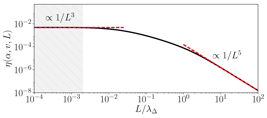
Figure 1: Correction factor $\eta$ as a function of the separation length $L$ measured in units of $\lambda_{\Delta}$. We have used the values $\alpha=1/137$ and $v=1/300$. The asymptotes, shown as red dashed lines, illustrate a scaling (of the Casimir energy) of $\propto L^{-3}$ for short separations ($L\ll\lambda_{\Delta}$) and $\propto L^{-5}$ for large separations ($L\gg\lambda_{\Delta}$). The gray hatched area corresponds to the regime for which the predictions of the Dirac model become less reliable – where we have choses $\lambda_{\rm Min}/\lambda_{\Delta}=2\times 10^{-3}$.

In the limit of large separations, i.e. for $\lambda\gg 1$, we have instead

$$\eta(\alpha,v,\lambda)\approx\frac{240\alpha^{2}}{\pi^{4}\lambda^{2}}\left[1+\frac{1}{15}\left(3+4v^{2}+3v^{4}\right)\right],$$ (8)

indicating a change in power-law behavior of the energy from $\propto L^{-3}$ to $\propto L^{-5}$ and showing that the presence of a band gap leads to a change of the Casimir force’s scaling that is accompanied by a reduction in magnitudes. This can be understood by considering that, at large separations, the Casimir effect effectively probes the low frequency optical response of the material: The presence of a band gap makes graphene a poor reflector at low energies. This behavior is, however, very different with respect to that of ordinary metals (which, for low frequencies, act as nearly perfect reflector) and explains the deviation from the $\propto L^{-3}$ power law. Still, the change in the exponent of the power-law is unusual: For ordinary materials, in going from the nonretarded to the retarded limit, the exponent usually changes by one unit due to the occurrence of the length scale provided by the plasma-frequency of the medium. This variation of two units in the exponent can, once again, directly be attributed to the different behavior of graphene’s reflection coefficients: For a nonzero gap, these coefficients feature a dielectric-like behavior with a reflectivity that vanishes in the limit $k,\omega\to 0$, while for ordinary metals it tends to a constant (see Appendix A).

IV Polaritonic Modes

For a single planar object, surface polariton modes are associated with resonances in the corresponding reflection coefficients. Consequently, their dispersion relation can be determined by solving $r^{-1}_{\sigma}(\omega,k)=0$. Since $\psi(p)$ is real for $p<1$ and larger than zero for $0<p<1$, we can infer from the expressions in Eq. (4) that, contrary to the usual behavior of ordinary metals, polaritonic modes only appear in the TE polarization. This leads to profound modifications of the electromagnetic field profiles that are connected with these excitations. For ordinary metals, the polaritonic resonances are typically associated with a TM-polarized field, which is predominantly electric. This property is related to the charge oscillations bounded to the surface (plasmons for metals) constituting the matter part of the polaritonic mode. Instead, a TE-polarized field is predominantly magnetic in nature. This behavior is connected with the statistically induced change in sign of the spinor loop which gives the polarization tensor for graphene bordag14 ; bordag15 . In Ref. mikhailov07 , where TE resonances were analyzed, this behavior has been associated with a change in sign of the interband contribution to graphene’s conductivity with respect to the behavior of the intraband conductivity of ordinary metals.

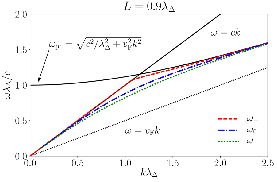
Figure 2: The dispersion relation of the single layer polariton $\omega_{0}(k)$ (blue dash-dotted line) and of the two coupled polaritons $\omega_{\pm}(k)$ (red dashed and green dotted lines) all lie below the pair-creation threshold $\omega_{\rm pc}(k)$. For better graphical representation the dispersion relations are plotted for the parameters $\alpha=v=1/2$. The antisymmetrically coupled polariton $\omega_{+}(k)$ (red dashed line) has to be continued with $\omega=ck$ starting from the point where it becomes tangent to the light cone, downward to zero.

The dispersion relation for the TE-polarized surface polariton of a single graphene layer can, in the $\Omega$-$K$ plane, be described in terms of the parametric curve

$$\Omega_{0}(K)\equiv\begin{cases}\Omega_{0}(\mu)=\sqrt{\frac{v^{2}\mu^{2}+\psi^{\rm iv}\left[\frac{\mu}{\alpha}\right]^{2}}{1-v^{2}}}\\ K_{0}(\mu)=\sqrt{\frac{\mu^{2}+\psi^{\rm iv}\left[\frac{\mu}{\alpha}\right]^{2}}{1-v^{2}}}\end{cases},$$ (9)

where $\psi^{\rm iv}$ denotes the inverse function of $\psi$, i.e. $\psi(\psi^{\rm iv}(x))=x$. Since for $v<1$ one has that $\Omega_{0}(\mu)\leq K_{0}(\mu)$, indicating that the field associated with this surface polariton is evanescent in agreement with $\mu\in(0,\infty)$. Furthermore, the resulting dispersion relation is bounded from above by the pair-creation threshold frequency $\Omega_{\mathrm{pc}}(K)$. These features are also clearly visible in Fig. 2. In particular, we observe that the polaritonic dispersion curve for the single graphene layer lies entirely below the light cone ($\omega=ck$ or equivalently $\mu=0$), goes to zero for small wavevectors and tends to the pair-creation frequency for large $k$. The behavior of the TE-polarized surface polariton has already been examined in great detail in the existing literature using a semi-analytical approach in Ref. bordag14 and using a parametric representation in Ref. Werra16 .

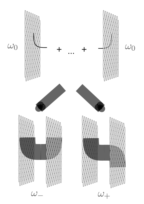
Figure 3: Schematic illustration of the setup analyzed in this work. The Casimir force between two identical, parallel, undoped graphene layers is considered. Particular attention is devoted to the polaritonic contribution. When the distance between the layers is reduced, the polaritons featured by each of the graphene layers start to interact. This interaction removes the degeneracy and the coupled modes are distinguished in terms of there associated field into a symmetric ($\omega_{-}$) and antisymmetric ($\omega_{+}$) coupled surface polariton.

In the case of two identical, parallel graphene sheets, the polaritonic excitations that live on each layer couple through their evanescent tails (see Fig. 3). In this case the dispersion relation of the corresponding coupled modes can be found from the solutions of

$$1-r_{\mathrm{TE}}^{2}(\omega,k)e^{-2\kappa L}=0\Rightarrow-r^{-1}_{\mathrm{TE}}(\omega,k)=\pm e^{-\mu\lambda}.$$ (10)

The solutions we are looking for must, in the limit $\lambda\to\infty$, tend to Eq. (9) since in this case the two sheets do not interact and the single layer case must be recovered. At finite separations, the interaction removes the degeneracy and two distinct coupled polaritons arise with a dispersion relation that also depends on the distance between the layers through the parameter $\lambda$. These coupled polaritons can be classified in terms of the properties of their electromagnetic field and we distinguish between an antisymmetric ($+$ sign) and a symmetric ($-$ sign) polaritonic excitation. Similar to the single layer case, their dispersion relations are given in terms of the parametric expressions

$$\Omega_{\pm}(K,\lambda)\equiv\begin{cases}\Omega_{\pm}(\mu,\lambda)=\sqrt{\frac{v^{2}\mu^{2}+\psi^{\rm iv}\left[\frac{\mu}{\alpha}f_{\pm}(\mu\lambda)\right]^{2}}{1-v^{2}}}\\ K_{\pm}(\mu,\lambda)=\sqrt{\frac{\mu^{2}+\psi^{\rm iv}\left[\frac{\mu}{\alpha}f_{\pm}(\mu\lambda)\right]^{2}}{1-v^{2}}}\end{cases},$$ (11)

where we have defined the function $f_{\pm}(x)=(1\mp e^{-x})^{-1}$. Since $f_{\pm}(x\to\infty)\sim 1$ at large separation, i.e. $\lambda\gg 1$, Eq. (11) approaches Eq. (9). The corresponding curves lie in the evanescent sector (i.e. below the light cone) and they are both bounded by the pair-creation threshold frequency to which they tend for $k\to\infty$. Further, the coupled modes obey the relation $\Omega_{-}(K)<\Omega_{0}(K)<\Omega_{+}(K)$. At small wave vectors, however, the two coupled modes behave in a very different way. The symmetric polariton frequency goes to zero for $k\to 0$ in a way similar to the single layer mode, although we always have $\Omega_{-}(K)<\Omega_{0}(K)$. Conversely, the $\Omega_{+}(K,\lambda)$ mode stops at

$$K\equiv K_{\mathrm{lc}}=\frac{\psi^{\rm iv}\left[\frac{1}{\alpha\lambda}\right]}{\sqrt{1-v^{2}}},$$ (12)

where, using the parametric expressions in Eq. (11), one can also show that the dispersion relation of the antisymmetric mode becomes tangent to the light cone (i.e. at this point, the group velocity is $c$). In the case of two metallic plates intravaia05 ; intravaia07 , the curve corresponding to $\Omega_{+}(K)$ continues above the light cone, indicating a change of the polaritonic field in the transverse direction from evanescent to propagating. For the graphene layers considered here, we find no propagating branch for the antisymmetric mode. This behavior is related to the mathematical properties of $\psi(p)$ in the propagating sector, below the pair-creation threshold – a solution would correspond to values for which $\mu$ is a purely imaginary number while $p<1$. This feature is similar to what was already observed for the polaritonic modes in a magneto-dielectric cavity Haakh13 . As in this case, the antisymmetric mode $\Omega_{+}(K)$ can be seen as departing from a continuum of TE-polarized waves occurring for $ck<\omega$ and are associated with the branch cut in the reflection coefficient due to the square root of $\kappa$. Note that the entire light cone ($\mu=0$) is a trivial, distance-independent solution of (10) that describes the antisymmetric polariton. Due to its properties and in order to preserve the number of modes as a function of the wave vector, analogous to Ref.  Haakh13 , we continue the $\Omega_{+}(K)$ dispersion relation along the light cone from $K=K_{\mathrm{lc}}$ down to zero (see Fig. 2). Starting from the above considerations, we calculate, in the next section, the contribution of surface polariton modes to the overall Casimir energy.

V Polaritonic contribution to the Casimir energy

In analogy to Eq. (1), we define the polaritonic contribution starting from the zero-point energy associated with the different modes:

$$E_{\mathrm{pol}}=\sum_{\textbf{k}}\left[\frac{\hbar\omega_{+}(\mathbf{k},L)}{2}+\frac{\hbar\omega_{-}(\mathbf{k},L)}{2}\right]_{L\rightarrow\infty}^{L}.$$ (13)

Using our dimensionless variables, this expression can be written as

$$\frac{E_{\mathrm{pol}}(\lambda)}{E_{\mathrm{N}}}=\int_{0}^{\infty}K\mathrm{d}K[\Omega_{+}(K,\lambda)+\Omega_{-}(K,\lambda)-2\Omega_{0}(K)],$$ (14)

where $E_{\mathrm{N}}=\hbar ck_{\Delta}^{3}A/(4\pi)$. Here, we have already considered that in the limit $L\rightarrow\infty$ the coupled modes tend to the single layer polariton. Owing to the implicit nature of the dispersion relations, this expression does not lend itself to a simple, straightforward evaluation. For our analytical and numerical investigations it is convenient to change the integration variable to $\mu$, which was used as parameter in Eqs. (9) and (11). Due to the Jacobian $K\mathrm{d}K=\mu\mathrm{d}\mu+\Omega\mathrm{d}\Omega$, the polaritonic energy can be written as

$$\frac{E_{\mathrm{pol}}(\lambda)}{E_{\mathrm{N}}}=\frac{1}{3}\left[\Omega_{+}^{3}+\Omega_{-}^{3}-2\Omega_{0}^{3}\right]_{K\rightarrow 0,K_{\mathrm{lc}}}^{K\rightarrow\infty}+\frac{1}{3}K_{\mathrm{lc}}^{3}\\ +\int_{0}^{\infty}\left[\Omega_{+}(\mu,\lambda)+\Omega_{-}(\mu,\lambda)-2\Omega_{0}(\mu)\right]\mu\mathrm{d}\mu.$$ (15)

In the first line, the upper limits cancel each other and the lower limit of $\Omega_{0}$ and $\Omega_{-}$ is zero. The remaining lower limit of $\Omega_{+}$ cancels the second term leaving us with

$$\frac{E_{\mathrm{pol}}(\lambda)}{E_{\mathrm{N}}}=\int_{0}^{\infty}\left[\Omega_{+}(\mu,\lambda)+\Omega_{-}(\mu,\lambda)-2\Omega_{0}(\mu)\right]\mu\mathrm{d}\mu.$$ (16)

This integral allows for a simpler analytical treatment and a robust numerical evaluation.

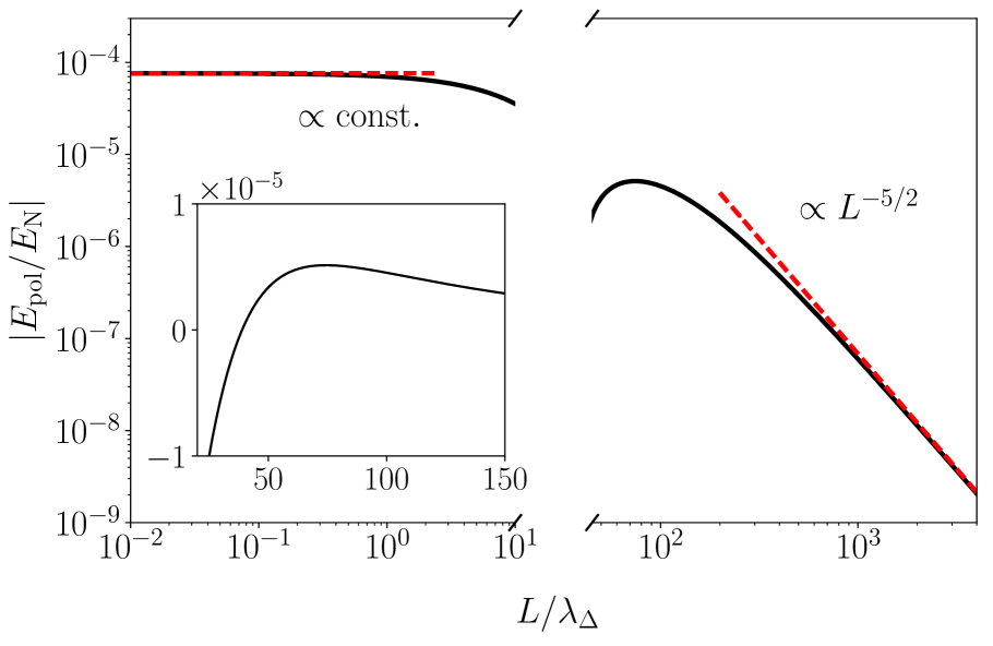
Figure 4: Absolute value of the polaritonic energy scaled to $E_{\mathrm{N}}$ as a function of the separation length in units of $\lambda_{\Delta}$. The asymptotes shown as red dashed lines illustrate a scaling of $\propto L^{-5/2}$ for large separations and a scaling of $\propto L^{0}$, i.e. a constant for vanishing separations. Inset: The polaritonic energy exhibits a maximum at $L\approx 74\lambda_{\Delta}$, where the behavior of the polaritonic modes changes from an attracting contribution to a repulsing one.

In Fig. 4, we depict the polaritonic energy in Eq. (16) and this highlights two important features of this contribution to the Casimir energy. First, in the case of two graphene layers and for $\lambda=L/\lambda_{\Delta}\ll 1$ the energy tends to a finite negative constant (see also Sec. V.1 below). When compared to the total energy discussed in Sec. III (see Fig. 1), this means that, contrary to the case of ordinary metals described via a spatially local dielectric model, where the plasmonic energy negatively diverges and dominates the Casimir interaction at short separations, for two graphene layers in close proximity, the surface polaritons provide only a sub-leading contribution to the total energy in Eq. (5). At this point we would like to emphasize that, different from the total energy, the polaritonic contribution is less sensitive to the minimal distance constraint discussed in Sec. III that has been derived from the range of validity of the Dirac model. Indeed, due to the low value of $v_{\rm F}/c$, the corresponding polaritonic energies, in the region where they contribute to the Casimir energy ($k\lesssim 1/L$), are limited by the pair-creation threshold. The means that the results are reliable for $L\gtrsim(v_{\rm F}/c)\lambda_{\rm Min}$.

Similar to the metallic case, the function $E_{\mathrm{pol}}(\lambda)$ increases with distance between the graphene layers and reaches a maximum at $L\approx 74\lambda_{\Delta}$. This indicates that the polaritonic contribution to the total force is attractive for distances shorter than this value and repulsive at larger separations. Interestingly, in this latter limit $E_{\mathrm{pol}}\propto L^{-5/2}$, which is the same scaling that have been observed for surface plasmon polaritons in the metallic case intravaia07 . These findings are also confirmed by the detailed asymptotic analysis reported below.

V.1 Asymptotic behaviors short and large separations

From a more mathematical point of view, the difference between the coupled and the isolated polaritons is due to the behavior of the function $f_{\pm}(x)$. Since $\psi^{\rm iv}\left[x\gg 1\right]\sim 1$, for $\lambda\ll 1$ we obtain the main contribution to the integral in Eq. (16) for $\mu\sim\alpha$. As a result, in the limit $\lambda\to 0$, we have

$$f_{+}(\mu\lambda)\approx\frac{1}{\mu\lambda}+\frac{1}{2}\gg 1,\quad f_{-}(\mu\lambda)\approx\frac{1}{2}.$$ (17)

In this limit, the expressions in the integrand of Eq. (16) thus become distance independent. Setting $x=\mu/\alpha$, the polaritonic energy approaches a constant given by

$$\frac{E_{\mathrm{pol}}(\lambda)}{E_{\mathrm{N}}}\xrightarrow{\lambda\to 0}\alpha^{2}\int_{0}^{\infty}\mathrm{d}x\,x\left[\sqrt{\frac{(\alpha v)^{2}x^{2}+1}{1-v^{2}}}\right.\\ \left.+\sqrt{\frac{(\alpha v)^{2}x^{2}+\psi^{\rm iv}\left[x/2\right]^{2}}{1-v^{2}}}-2\sqrt{\frac{(\alpha v)^{2}x^{2}+\psi^{\rm iv}\left[x\right]^{2}}{1-v^{2}}}\right].$$ (18)

This expression scales with $\alpha^{2}$ and is only weakly depending on $v$. Using $\alpha=1/137$ and $v=1/300$ gives $E_{\mathrm{pol}}/E_{\mathrm{N}}\approx-7.6\times 10^{-5}$.

For larger separations, the dispersion relations of the coupled polaritonic modes are very close to the uncoupled one. The difference is controlled by the small parameter $e^{-\mu\lambda}$ which is significant only for $\mu\lesssim 1/\lambda$. In the limit $1/\lambda\to 0$ we may then neglect the first term under the square roots in Eqs. (9) and (11) and consider that $\psi^{\rm iv}(x\rightarrow 0)\approx\sqrt{3x}/2$. We then have

$$\Omega_{\pm}(\mu,\lambda)-\Omega_{0}(\mu)\approx\sqrt{\frac{3\frac{\mu}{\alpha}}{1-v^{2}}}\frac{\sqrt{f_{\pm}(\mu\lambda)}-\sqrt{f_{0}(\mu\lambda)}}{2}.$$ (19)

Inserting the previous expressions in Eq. (16) and employing a change of variable $x=\mu\lambda$, it is straightforward to show that, for large distances, the polaritonic energy goes as

$$\frac{E_{\mathrm{pol}}(\lambda\gg 1)}{E_{\mathrm{N}}}\approx\sqrt{\frac{3}{4\alpha(1-v^{2})}}\frac{C}{\lambda^{5/2}},$$ (20)

where $C$ is a numerical constant given by

$$C =\int_{0}^{\infty}\mathrm{d}x\,x^{\frac{3}{2}}\Bigg{\{}\sqrt{\frac{1+\tanh\left[\frac{x}{2}\right]}{2}}+\sqrt{\frac{1+\coth\left[\frac{x}{2}\right]}{2}}-2\Bigg{\}}$$

$$\approx 0.2132.$$ (21)

The polaritonic modes thus give a contribution to the energy which is positive and vanishes slower than the total energy ($E(L)\propto L^{-5}$).

VI Discussion and conclusions

In this work, we have analyzed in detail the contribution of surface polaritons to the zero-temperature Casimir interaction between two parallel graphene layers that are separated by vacuum and are described by the Dirac model. In our description we include a small gap in the band structure of graphene that accounts for the effect of strain or other experimental conditions which can lead to a breaking of symmetry in the material’s lattice structure.

Specifically, we have derived parametric expressions for the two coupled surface modes that result from the hybridization of the two single-layer polaritons and have calculated their contribution to the Casimir energy. For the parameters considered ($T=0$ and vanishing chemical potential), the system only allows for TE-polarized surface resonances. Despite the complexity of the expressions, our approach has allowed for a detailed analytical description of the polaritonic energy. We have shown that all modes are associated with an evanescent field: the dispersion relations of the single-layer $\omega_{0}(k)$ and the symmetric coupled mode $\omega_{-}(k)$ tend to zero for $k\to 0$; the remaining antisymmetric coupled mode $\omega_{+}(k)$ becomes instead tangent to the light cone for a positive and distance dependent value of the wave vector. A similar behavior was observed in the case of the surface polaritons occurring in a magneto-dielectric cavity Haakh13 .

Further, we have analyzed the behavior of the polaritonic contribution for small and large separations $L$ between the layers and have contrasted the resulting expressions with those for the total Casimir energy. Contrary to ordinary metals, for which the polaritonic contribution describes the nonretarded short-distance behavior (van der Waals limit), the total energy for graphene scales $\propto L^{-3}$ while the surface modes’ energy tends to a constant. Due to the band gap, at large distances the total zero-temperature Casimir energy exhibits an unusual $L^{-5}$ behavior, while the polaritonic energy scales as $\propto L^{-5/2}$, similar to that found for the corresponding contribution in the case of two metallic plates intravaia05 ; bordag06 ; intravaia07 . In analogy with this last configuration, the polaritonic Casimir energy has the interesting property to exhibit a maximum at a distance which for graphene scales as the inverse of the bandgap energy. Consequently, the polaritonic force changes sign and being attractive at short separations and becoming repulsive at large separations. Nonetheless, the total Casimir force remains attractive throughout.

Our results show that, in the technologically interesting limit of very small separations (van der Waals solids), graphene’s surface resonances can behave in a quite unusual way relative to the analogous situation for ordinary metals.

VII Acknowledgments

We are indebted with I. G. Pirozhenko, D. Reiche and M. Oelschläger for insightful and fruitful discussions. Further, we acknowledge support by the Deutsche Forschungsgemeinschaft (DFG) through SFB 951 HIOS (B10, Project No. 182087777). FI acknowledges financial support from the DFG through the DIP program (Grant No. SCHM 1049/7-1).

Appendix A The impact of graphene’s onto-electronic properties on the Casimir energy

As explained in the main text, in order to investigate the Casimir energy between two parallel graphene sheets, it is convenient to use the function $\eta(\alpha,v,\lambda)$, which compares the Casimir energy with the energy between two perfectly reflecting surfaces. With the change of variable $\tilde{\xi}=2\lambda\xi\lambda_{\Delta}/c$ and $\tilde{k}=2\lambda k\lambda_{\Delta}$, we may write the reflection coefficients as

$$r_{\textrm{TE}}(\mathrm{i}\tilde{\xi},\tilde{k})=-\frac{2\lambda\alpha\varphi\left(\frac{\tilde{\rho}}{2\lambda}\right)}{\tilde{\kappa}+2\lambda\alpha\varphi\left(\frac{\tilde{\rho}}{2\lambda}\right)},$$ (22a)

$$r_{\textrm{TM}}(\mathrm{i}\tilde{\xi},\tilde{k})=\frac{2\lambda\alpha\tilde{\kappa}\varphi\left(\frac{\tilde{\rho}}{2\lambda}\right)}{2\lambda\alpha\tilde{\kappa}\varphi\left(\frac{\tilde{\rho}}{2\lambda}\right)+\tilde{\rho}^{2}},$$ (22b)

where $\tilde{\kappa}=\sqrt{\tilde{k}^{2}+\tilde{\xi}^{2}}$, $\tilde{\rho}=\sqrt{\tilde{\xi}^{2}+v^{2}\tilde{k}^{2}}$ and

$$\varphi(x)\equiv-\psi(\mathrm{i}x)=\left[1+\left(x-\frac{1}{x}\right)\arctan\left(x\right)\right].$$ (23)

In this case, the function $\eta(\alpha,v,\lambda)$ can be written as follows

$$\eta(\alpha,v,\lambda)=-\frac{45}{2\pi^{4}}\int_{0}^{\infty}\mathrm{d}\tilde{\xi}\int_{0}^{\infty}\mathrm{d}\tilde{k}\,\tilde{k}\\ \sum_{\sigma}\ln\left[1-r^{2}_{\mathrm{\sigma}}(\mathrm{i}\tilde{\xi},\tilde{k})_{|\lambda\rightarrow 0}e^{-\tilde{\kappa}}\right]$$ (24)

Due to the exponential in the integrand the dominant contributions arise for $1\gtrsim\tilde{\kappa}>\tilde{\rho}$.

In the limit $\lambda\to 0$ we can, therefore, consider the limit $\varphi(x)\approx x\pi/2$ that is obtained for $x\to\infty$. In this case, the resulting expressions for the reflection coefficients are the same as those that are obtained for the limit $\Delta\to 0$

$$r_{\textrm{TE}}(\mathrm{i}\tilde{\xi},\tilde{k})\approx-\frac{\alpha\frac{\pi}{2}\tilde{\rho}}{\tilde{\kappa}+\alpha\frac{\pi}{2}\tilde{\rho}},\quad r_{\textrm{TM}}(\mathrm{i}\tilde{\xi},\tilde{k})\approx\frac{\alpha\tilde{\kappa}\frac{\pi}{2}}{\alpha\tilde{\kappa}\frac{\pi}{2}+\tilde{\rho}}.$$ (25)

As a consequence, the function $\eta(\alpha,v,\lambda)$ does not depend on $\lambda$. The above expressions also show that, in this limit, the TM contribution is larger than the TE contribution. In order to obtain an analytically tractable expression, we introduce polar coordinates in the $\tilde{\xi}$-$\tilde{k}$-plane, $\tilde{\xi}=h\sin[\phi]$ and $\tilde{k}=h\cos[\phi]$, and simplify the integration over the angle through the change of variable $x=\sin\phi$. The integral can then be solved analytically but features rather lengthy expressions, the full form of which we do not want to give here. We have

$$\eta(\alpha,v,0)\approx\frac{45}{\pi^{4}}\left[g_{\mathrm{TE}}(\alpha,v)+g_{\mathrm{TM}}(\alpha,v)\right],$$ (26)

where

$$g_{\mathrm{TE}}(\alpha,v)=\int_{0}^{1}\mathrm{d}x\left(\frac{\frac{\alpha\pi}{2}\sqrt{x^{2}(1-v^{2})+v^{2}}}{1+\frac{\alpha\pi}{2}\sqrt{x^{2}(1-v^{2})+v^{2}}}\right)^{2}$$ (27)

and

$$g_{\mathrm{TM}}(\alpha,v)=\int_{0}^{1}\mathrm{d}x\left(\frac{1}{1+\frac{2}{\alpha\pi}\sqrt{x^{2}(1-v^{2})+v^{2}}}\right)^{2}.$$ (28)

Further, we observe that for very small $\alpha$, we can Taylor-expand the expression

$$\eta(\alpha,v,0)\stackrel{{\scriptstyle\alpha\ll 1}}{{\approx}}\frac{45}{4\pi^{2}}\alpha^{2}\left(\frac{1}{3}\left(2v^{2}+1\right)+\frac{\arctan\left(\sqrt{\frac{1-v^{2}}{v^{2}}}\right)}{\sqrt{v^{2}\left(1-v^{2}\right)}}\right)$$ (29)

and obtain a scaling $\eta\propto\alpha^{2}$.

For $\lambda\gg 1$, we can use the approximation $\varphi(x)\approx 4x^{2}/3$ valid for $x\ll 1$. The reflection coefficients then become

$$r_{\textrm{TE}}(\mathrm{i}\tilde{\xi},\tilde{k})\approx-\frac{2}{3}\frac{\alpha}{\lambda}\frac{\tilde{\rho}^{2}}{\tilde{\kappa}},\quad r_{\textrm{TM}}(\mathrm{i}\tilde{\xi},\tilde{k})\approx\frac{2}{3}\frac{\alpha}{\lambda}\tilde{\kappa}$$ (30)

Similarly to the previous case, we consequently have

$$\eta(\alpha,v,\lambda) \stackrel{{\scriptstyle\lambda\gg 1}}{{\approx}}\frac{\alpha^{2}}{\lambda^{2}}\frac{10}{\pi^{4}}\int_{0}^{\infty}\mathrm{d}\tilde{\xi}\int_{0}^{\infty}\mathrm{d}\tilde{k}\,\tilde{k}\left[\tilde{\kappa}^{2}-\frac{\tilde{\rho}^{4}}{\tilde{\kappa}^{2}}\right]e^{-\tilde{\kappa}}$$

$$=\frac{240\alpha^{2}}{\pi^{4}\lambda^{2}}\left[1+\frac{1}{15}\left(3+4v^{2}+3v^{4}\right)\right].$$ (31)

References

- (1) H. B. G. Casimir, On the attraction between two perfectly conducting plates, Proc. K. Ned. Akad. Wet. 51, 793 (1948).
- (2) N. van Kampen, B. Nijboer, and K. Schram, On the macroscopic theory of Van Der Waals forces, Phys. Lett. A 26, 307 (1968).
- (3) C. Henkel, K. Joulain, J.-P. Mulet, and J.-J. Greffet, Coupled surface polaritons and the Casimir force, Phys. Rev. A 69, 023808 (2004).
- (4) F. Intravaia and A. Lambrecht, Surface Plasmon Modes and the Casimir Energy, Phys. Rev. Lett. 94, 110404 (2005).
- (5) G. Barton, Casimir effects for a flat plasma sheet: I. Energies, J. Phys. A Math. Gen. 38, 2997 (2005).
- (6) M. Bordag, The Casimir effect for thin plasma sheets and the role of the surface plasmons, J. Phys. A Math. Gen. 39, 6173 (2006).
- (7) F. Intravaia, C. Henkel, and A. Lambrecht, Role of surface plasmons in the Casimir effect, Phys. Rev. A 76, 033820 (2007).
- (8) H. R. Haakh, S. Faez, and V. Sandoghdar, Polaritonic normal-mode splitting and light localization in a one-dimensional nanoguide, Phys. Rev. A 94, 053840 (2016).
- (9) E. N. Economou, Surface Plasmons in Thin Films, Phys. Rev. 182, 539 (1969).
- (10) K. Joulain, J.-P. Mulet, F. Marquier, R. Carminati, and J.-J. Greffet, Surface electromagnetic waves thermally excited: Radiative heat transfer, coherence properties and Casimir forces revisited in the near field, Surface Science Reports 57, 59 (2005).
- (11) J. M. Pitarke, V. M. Silkin, E. V. Chulkov, and P. M. Echenique, Theory of surface plasmons and surface-plasmon polaritons, Rep. Prog. Phys. 70, 1 (2007).
- (12) S. A. Maier, Plasmonics: fundamentals and applications (Springer Science and Business Media, New York, 2007).
- (13) S. Nie and S. Emory, Probing single molecules and single nanoparticles by surface-enhanced Raman scattering, Science 275, 1102 (1997).
- (14) T. Ebbesen, H. Lezec, H. Ghaemi, T. Thio, and P. Wolff, Extraordinary optical transmission through sub-wavelength hole arrays, Nature 391, 667 (1998).
- (15) P. Törmä and W. L. Barnes, Strong coupling between surface plasmon polaritons and emitters: a review, Rep. Prog. Phys. 78, 013901 (2015).
- (16) F. Intravaia, P. S. Davids, R. S. Decca, V. A. Aksyuk, D. López, and D. A. R. Dalvit, Quasianalytical modal approach for computing Casimir interactions in periodic nanostructures, Phys. Rev. A 86, 042101 (2012).
- (17) F. Intravaia et al., Strong Casimir force reduction through metallic surface nanostructuring, Nat. Commun. 4, 2515 (2013).
- (18) I. V. Fialkovsky, V. N. Marachevsky, and D. V. Vassilevich, Finite-temperature Casimir effect for graphene, Phys. Rev. B 84, 035446 (2011).
- (19) A. A. Banishev, G. L. Klimchitskaya, V. M. Mostepanenko, and U. Mohideen, Demonstration of the Casimir Force between Ferromagnetic Surfaces of a Ni-Coated Sphere and a Ni-Coated Plate, Phys. Rev. Lett. 110, 137401 (2013).
- (20) S.-A. Biehs and G. S. Agarwal, Anisotropy enhancement of the Casimir-Polder force between a nanoparticle and graphene, Phys. Rev. A 90, 042510 (2014).
- (21) G. L. Klimchitskaya and V. M. Mostepanenko, Comparison of hydrodynamic model of graphene with recent experiment on measuring the Casimir interaction, Phys. Rev. B 91, 045412 (2015).
- (22) G. L. Klimchitskaya and V. M. Mostepanenko, Origin of large thermal effect in the Casimir interaction between two graphene sheets, Phys. Rev. B 91, 174501 (2015).
- (23) M. Bordag, I. Fialkovskiy, and D. Vassilevich, Enhanced Casimir effect for doped graphene, Phys. Rev. B 93, 075414 (2016).
- (24) C. Henkel, G. L. Klimchitskaya, and V. M. Mostepanenko, Influence of the chemical potential on the Casimir-Polder interaction between an atom and gapped graphene or a graphene-coated substrate, Phys. Rev. A 97, 032504 (2018).
- (25) G. L. Klimchitskaya and V. M. Mostepanenko, Graphene may help to solve the Casimir conundrum in indium tin oxide systems, Phys. Rev. B 98, 035307 (2018).
- (26) A. K. Geim and I. V. Grigorieva, Van der Waals heterostructures, Nature 499, 419 EP (2013).
- (27) V. V. Gobre and A. Tkatchenko, Scaling laws for van der Waals interactions in nanostructured materials, Nat. Commun. 4, (2013).
- (28) K. S. Novoselov, A. Mishchenko, A. Carvalho, and A. H. Castro Neto, 2D materials and van der Waals heterostructures, Science 353, (2016).
- (29) A. Ambrosetti, N. Ferri, R. A. DiStasio, and A. Tkatchenko, Wavelike charge density fluctuations and van der Waals interactions at the nanoscale, Science 351, 1171 (2016).
- (30) L. M. Woods, D. A. R. Dalvit, A. Tkatchenko, P. Rodriguez-Lopez, A. W. Rodriguez, and R. Podgornik, Materials perspective on Casimir and van der Waals interactions, Rev. Mod. Phys. 88, 045003 (2016).
- (31) E. McCann, in Graphene Nanoelectronics, NanoScience and Technology, edited by H. Raza (Springer, Berlin Heidelberg, 2012), pp. 237–275.
- (32) J. F. M. Werra, F. Intravaia, and K. Busch, TE resonances in graphene-dielectric structures, J. Opt. 18, 034001 (2016).
- (33) S. Y. Zhou et al., Substrate-induced bandgap opening in epitaxial graphene, Nat. Mater. 6, 770 (2007).
- (34) G. Giovannetti, P. A. Khomyakov, G. Brocks, P. J. Kelly, and J. van den Brink, Substrate-induced band gap in graphene on hexagonal boron nitride: Ab initio density functional calculations, Phys. Rev. B 76, 073103 (2007).
- (35) Z.-G. Chen et al., Observation of an intrinsic bandgap and Landau level renormalization in graphene/boron-nitride heterostructures, Nat. Commun. 5, (2014).
- (36) J. Jung, A. M. DaSilva, A. H. MacDonald, and S. Adam, Origin of band gaps in graphene on hexagonal boron nitride, Nat. Commun. 6, (2015).
- (37) M. Chaichian, G. L. Klimchitskaya, V. M. Mostepanenko, and A. Tureanu, Thermal Casimir-Polder interaction of different atoms with graphene, Phys. Rev. A 86, 012515 (2012).
- (38) L. A. Falkovsky and A. A. Varlamov, Space-time dispersion of graphene conductivity, Eur. Phys. J. B 56, 281 (2007).
- (39) L. A. Falkovsky, Optical properties of graphene, J. Phys. Conf. Ser. 129, 012004 (2008).
- (40) M. Bordag and I. G. Pirozhenko, Surface plasmons for doped graphene, Phys. Rev. D 91, 085038 (2015).
- (41) E. Lifshitz, The Theory of Molecular Attractive Force between Solids, Soviet Phys. JETP 2, 73 (1956).
- (42) C. Genet, A. Lambrecht, and S. Reynaud, Casimir force and the quantum theory of lossy optical cavities, Phys. Rev. A 67, 043811 (2003).
- (43) G. L. Klimchitskaya and V. M. Mostepanenko, van der Waals and Casimir interactions between two graphene sheets, Phys. Rev. B 87, 075439 (2013).
- (44) M. Bordag and I. G. Pirozhenko, Transverse-electric surface plasmon for graphene in the Dirac equation model, Phys. Rev. B 89, 035421 (2014).
- (45) S. A. Mikhailov and K. Ziegler, New Electromagnetic Mode in Graphene, Phys. Rev. Lett. 99, 016803 (2007).
- (46) H. R. Haakh and F. Intravaia, Mode structure and polaritonic contributions to the Casimir effect in a magnetodielectric cavity, Phys. Rev. A 88, 052503 (2013).