Deep Classification Network for Monocular Depth Estimation

Abstract

Monocular Depth Estimation is usually treated as a supervised and regression problem when it actually is very similar to semantic segmentation task since they both are fundamentally pixel-level classification tasks. We applied depth increments that increases with depth in discretizing depth values and then applied Deeplab v2 [1] and the result was higher accuracy. We were able to achieve a state-of-the-art result on the KITTI dataset[2] and outperformed existing architecture by an 8% margin.

Keywords Depth Estimation  $\cdot$ Semantic Segmentation

1 Introduction

Generally trying to get 3D information from 2D images can be very challenging. This is because no exact solution exists, many 3D images could have produced the same 2D information. The task can feel like trying to create information from nothing. A task that is like that is Monocular depth estimation. It is a task that involves estimating depth from a single image rather than stereo pairs, which is what we’re investigating in this paper.

Depth estimation is an easier problem to track using stereo pairs [3]. However, it is easy to now see it as a supervised learning challenge since ground truth depth maps could be obtained from stereo pairs and used to train models and predict depths [4]. So deep convolutional networks can be used for building large networks that can predict depth maps [5].

Our proposal is that depth estimation can be formulated as a pixel-level classification task similar to the semantic segmentation task. So a state-of-the-art architecture already performing well in semantic segmentation can be used for depth estimation. Depth values could be discretized so they have pixel-level classes just like in segmentation. We, therefore, applied spatially increasing discretization (SID) on the depth values. SID converts depth values to the logarithm scale, divides the range of values equally and then converts it back.

The remaining sections in this paper are organized as follows. Relevant literature is first reviewed in Sec. 2, then the proposed method is discussed in Sec. 3. In Sec. 4 We explore the performance of our proposed method through experiments and we finally conclude in Sec. 5

2 Related Work

Depth Estimation usually involves trying to estimate dense or sparse depth map given images. A common approach usually involves using stereo images. Points of correspondence are located in the stereo pairs and then depth is estimated by triangulation. [3] did a taxonomy of stereo correspondence algorithms by comparing the performance of existing algorithms. It is also possible to learn depth estimation if it’s posed as a supervised learning problem [4]. The labels are usually monocular cues in 2D images [6] [7] [8]. Markov Random Fields (MRFs) is usually used for getting global cues since some of the former features were merely local cues. MRF and supervised learning was used in Make3D [9]. [10] also gets global cues using Depth Transfer, which involves finding similar image in an already existing databases of images to the input image, then warping the candidate image and depth to align with the input image and finally using an optimization procedure to interpolate and smoothen the candidate depth values.

Using deep convolutional networks like VGG [11] and ResNet [12], depth estimation performance has improved. [5] used a multi-scale network to predict depth, estimate surface normal and for semantic segmentation. [13] discretized depth with spatially increasing discretization (SID) and recast depth estimation as an ordinal regression problem.

Semantic Segmentation is a task where the aim is to predict the class each pixel of an image belongs to. A popular approach in this area is the use of a fully convolutional network (FCN) for prediction [14]. A much more advanced approach is Deeplab v2 [1]. Input images were passed through a layer of atrous (dilated) convolutional network which helps with adjusting the field of view and control the resolution of the feature map generated by a deep convolutional neural network. A coarse score map is then produced which undergoes bilinear interpolation for upsampling and finally fully connected conditional random field (CRF) is used as a post-processing process which helps incorporate low-level details in the segmentation result since skip connections are not used here. In an attempt to close domain gaps, the main idea has been to reduce the gap between source and target distribution by learning embeddings that are invariant to domains such as in Deep Adaptation Network (DAN) architecture which generalizes simple convolutional network tasks to fit for domain adaptation [15]. The base convolutional neural network for Deeplab v2 is ResNet101 [12] which has been pretrained on Imagenet dataset [16] through transfer learning technique [17].

Domain Adaptation involves trying to learn from a source distribution and predict on a target distribution. It is unsupervised when the source is labeled while the target is not. Deep Adaptation Network (DAN) tries to learn transferable features in task-specific layers which help generalize CNN for domain adaptation [18]. Deep CORAL can help unsupervised domain adaptation by aligning correlation of activation layers [19].

Adaptation for Depth Estimation involves reducing the domain gap between a source distribution (usually a synthetic dataset) and a target distribution (usually a real dataset) while trying to accomplish the task of unsupervised depth estimation in the unlabeled target domain. There are some important recent works in this aspect. AdaDepth (Adaptation for depth estimation) uses a residual encoder-decoder architecture with adversarial set up to accomplish a pixel-wise regression task of monocular depth estimation [20]. [21] accomplishes the same task by combining adversarial techniques and style transfer. GASDA (Geometry-Aware Symmetric Domain Adaptation Network) is an architecture that exploits epipolar geometry in the target domain and labels in the source domain[22].

3 Methods

This section first introduces the base architecture which was originally designed and is usually used for semantic segmentation and then how it was adapted for depth estimation by discretizing continuous depth ground truth. Each depth range is then treated as a class for semantic segmentation.

3.1 Deeplab for Semantic Segmentation

The base network used for this project is Deeplab v2. Prior to Deeplab, Fully connected convolutional networks were used for semantic segmentation [23]. They had a prominent feature which was skip-connections, which involves feeding the output of one layer as an input to another layer skipping some layers in between. FCN-8 has 2 skip connections, FCN-16 has 1 and FCN-32 has none. The skip connections help with incorporating low-level details to the results of semantic segmentation. Deeplab v2 had some important features as shown in Figure LABEL:fig:deeplab.

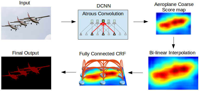
Figure 1: Deeplab [1]. An input image is passed through a Deep Convolutional Neural Network(DCNN) such as ResNet101, using atrous convolution to reduce downsampling. The score map output is then interpolated for upsampling to original image resolution. Low-level details are finally incorporated with the final result through a pre-processing step of fully connected conditional random field (CRF)

Atrous convolution helps with adjusting the field of view and controlling the resolution of the feature map generated by a deep convolutional neural network.

Bilinear interpolation is used for upsampling and Fully connected CRF is done as a post-processing process which helps incorporated low-level details in the segmentation result since skip connections are not used here.

ASPP (Atrous spatial pyramid pooling) helps handle scale variability in semantic segmentation by adjusting the resolution of feature maps by applying various atrous rates and fusing the result.

3.2 Spatially-Increasing Discretization

Figure 2: Intervals. UD (middle) and SID (bottom) to discretize depth interval [$\alpha,\beta$]

into sub intervals $d_{i}$ where $i=0,1,2,...K$ and K = number of class. UD is Uniform Discretization, SID is spatially increasing interval discretization

In order to properly frame depth estimation as a pixel-level classification problem which is exactly how semantic segmentation is done, then there’s a need to discretize continuous depth values. This is done such that each bin of depth values can be treated as a class of its own. Two common methods used to discretize continuous depth values are uniform discretization (UD) and spatially increasing interval discretization (SID). Uniform discretization just divides the space between the interval [$\alpha,\beta$] equally as shown in Fig 2. To divide the interval [$\alpha,\beta$] into K classes, UD can be formulated as:

$$d_{i}=\alpha+(\beta-\alpha)*\frac{i}{K},i=0,1,...,K$$ (1)

where $d_{i}\in{d_{0},d_{1},...,d_{K}}$ are depth interval boundaries. One challenge of using UD for discretization is that large depth values like the pixels belonging to the class "sky" will correspond to too many intervals or equivalently too many values. They could become really noisy and influence the loss. One of the common ways of handling outliers is to apply a log function to them. This means log function is applied to the continuous depth values and then divided equally in the interval [$\alpha,\beta$]. This is exactly what SID addresses. We still however treated depth values larger than 80m. Using SID to divide the interval [$\alpha,\beta$] into K classes, we can formulate it as:

$$d_{i}=\exp(\log{\alpha}+\frac{\log{\beta/\alpha}*i}{K}),i=0,...,K$$ (2)

where $d_{i}\in{d_{0},d_{1},...,d_{K}}$ are depth interval boundaries.

4 Experiments

We now discuss the implementation details of our experiment, and our evaluation on two datasets KITTI [2] and SYNTHIA [24].

Implementation details We used the publicly available deep learning framework pytorch [25]. Using ResNet-101 [12] as our feature extractor with Imagenet-pretrained weights, our model is trained for 100K iterations for KITTI and SYNTHIA with a batch size of 3 and initial learning rate of 0.00025 which applies a polynomial decay with the power of 0.9. We used weight decay of 0.0005 and momentum of 0.9. Eigen test split, the data augmentation techniques from [26] was used. Our model was trained on a 12gb RAM NVIDIA TITAN Xp GPU.

	Higher is better			Lower is better
Method	$\delta<1.25$	$\delta<1.25^{2}$	$\delta<1.25^{3}$	Abs Rel	RMSE	$RMSE_{log}$
Make3D[27]	0.601	0.820	0.926	0.280	8.734	0.361
Eigen et al.[26]	0.692	0.899	0.967	0.190	7.156	0.270
Liu et al.[28]	0.647	0.882	0.961	0.217	6.986	0.289
LRC (CS + K)[29]	0.861	.949	0.976	0.114	4.935	0.206
Kuznietsov et al.[30]	0.862	0.960	0.986	.113	4.621	0.189
DORN (VGG)[13]	0.915	0.980	0.993	0.081	3.056	0.132
DORN (ResNet)[13]	0.932	0.984	0.994	0.072	2.727	0.120
Ours(ResNet)	0.796	0.985	1.000	0.075	2.499	0.156

Table 1: Performance on KITTI. K is KITTI, CS is Cityscapes. $1.25$, $1.25^{2}$ and $1.25^{3}$ are pre-defined thresholds for Accuracy under threshold metric ($\delta$)

	Higher is better			Lower is better
Method	$\delta<1.25$	$\delta<1.25^{2}$	$\delta<1.25^{3}$	Abs Rel	RMSE	$RMSE_{log}$
Ours(ResNet)	0.785	0.937	0.945	0.108	9.270	0.206

Table 2: Performance on SYNTHIA.$1.25$, $1.25^{2}$ and $1.25^{3}$ are pre-defined thresholds for Accuracy under threshold metric ($\delta$)

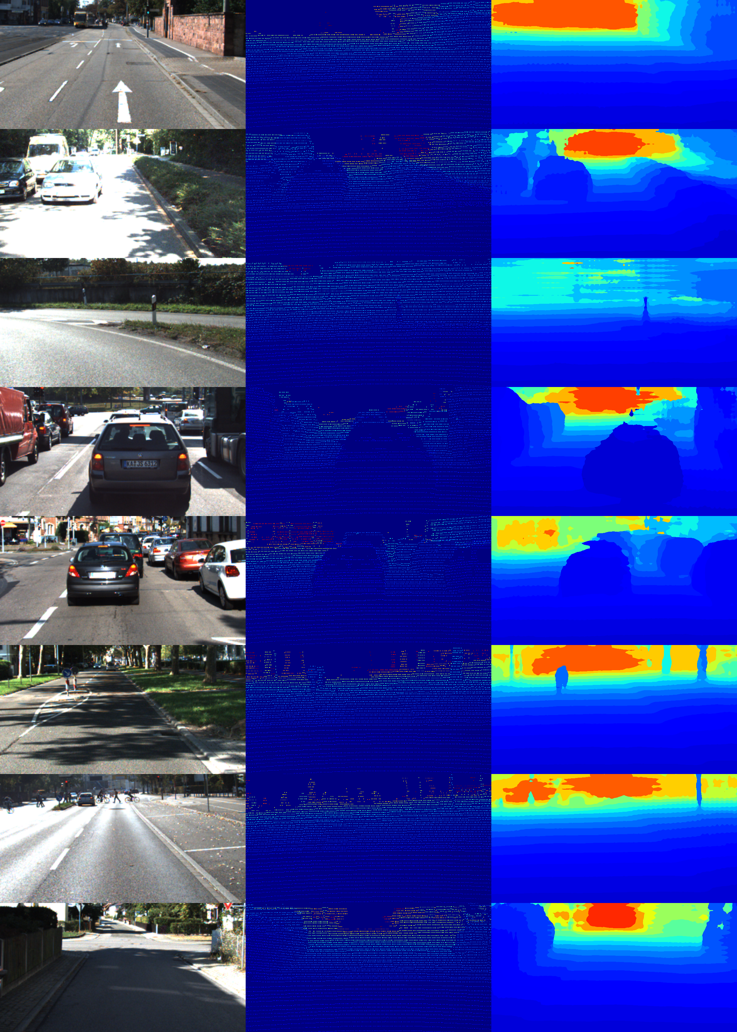
Figure 3: Depth Predictions on KITTI. The Image on the left column, ground truth in the middle and our model prediction on the right. The color color bar below shows the range of depths. Blue is nearer.

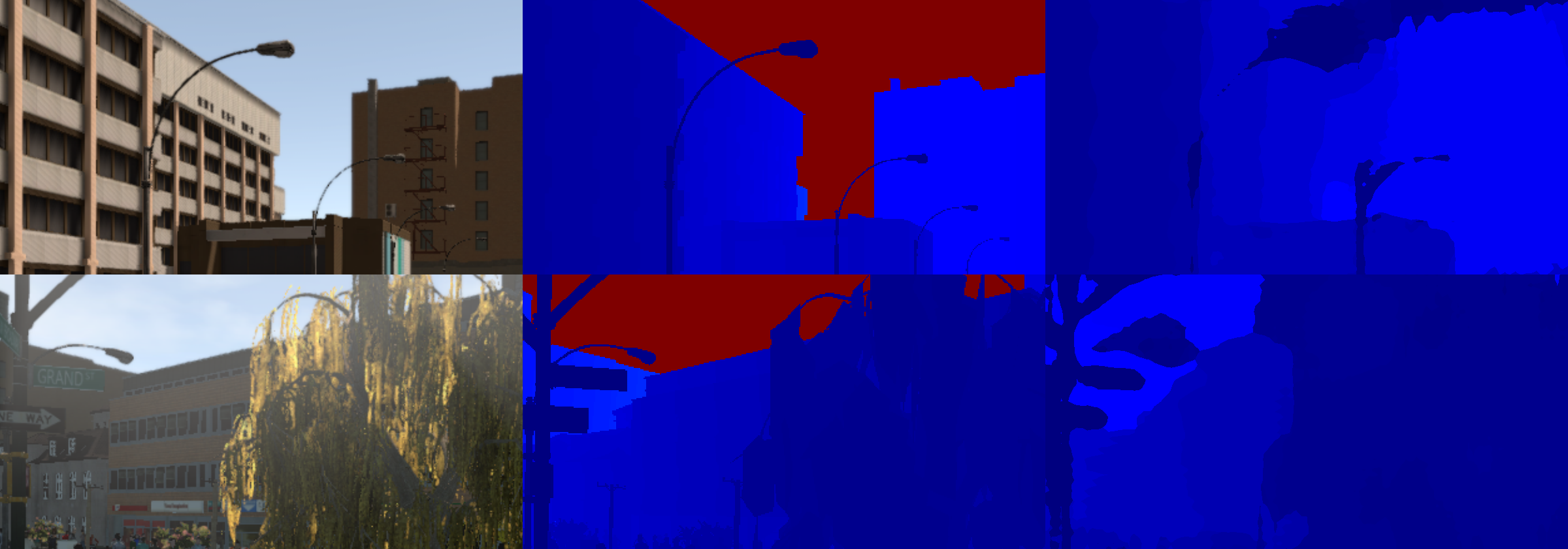
Figure 4: Depth Predictions on SYNTHIA. The Image on the left column, ground truth in the middle and our model prediction on the right. The color color bar below shows the range of depths. Blue is nearer.

4.1 Benchmark Performance

KITTI The KITTI dataset [2] contains images from cameras and depth sensors collected from a car. There are 61 total scenes. We used 23488 images from 32 scenes for training and 697 images from 29 scenes for testing [26]. The images were cropped to 420 x 800. We used SID to discretize the depth maps into 71 classes and ignored depth values beyond 80m during network loss calculations.

SYNTHIA We used the SYNTHIA dataset [24] because it’s synthetic. We used the SYNTHIA-RAND-CITYSCAPES subset which has 9,400 labeled images. We also cropped to 420 x 800 for training and testing. Depth map was also discretized to 71 classes and depth values beyond 80m were also ignored.

Performance Table 1 shows the result of our performance compared to other existing models on KITTI. The metrics used for comparison are standards compared in [31]. Letting $\hat{d}_{p}$ and $d_{p}$ denote estimated and ground truth depths respectively at pixel $p$, T denote total number of pixels, the metrics used were calculated thus:

Absolute Relative Error [9],

$$absRel=\frac{1}{T}\sum_{p}\frac{|d_{p}-\hat{d}_{p}|}{d_{p}}$$ (3)

Root Mean Square Error [32],

$$RMSE=\sqrt{\frac{1}{T}\sum_{p}(d_{p}-\hat{d}_{p})^{2}}$$ (4)

log scale invariant Root Mean Square Error [26],

$$RMSE_{log}=\frac{1}{T}\sum_{p}(\log{\hat{d}_{p}}-\log{d_{p}}+\alpha(\hat{d}_{p},d_{p}))^{2}$$ (5)

where $\alpha(\hat{d}_{p},d_{p})$ addresses scale alignment.

Accuracy under a threshold [7]

$$\delta<th=max(\frac{\hat{d}_{p}}{d_{p}},\frac{d_{p}}{\hat{d}_{p}})$$ (6)

where th is a predefined threshold, we used $1.25$, $1.25^{2}$ and $1.25^{3}$

We were able to get $\sim 8\%$ improve in accuracy in terms of root mean squared error metrics. Our model also performed better in other metrics. Table 2 also shows the result of our model’s performance on SYNTHIA. Qualitative results are also shown in Figures 3 and 4. The results demonstrate that our model is applicable to outdoor data and synthetic dataset.

5 Conclusion

We’ve been able to demonstrate how a depth estimation task can be formulated as a semantic segmentation problem since the two tasks are fundamentally just pixel-level classification tasks at the core. Simply discretizing the depth map and treating the binned depths as classes and applying a state-of-the-art semantic segmentation network can produce a result that outperforms existing results. In the future, we would investigate domain gaps in monocular depth maps estimation and apply class balanced self training[33] to attempt to reduce the gap.

References

- [1] Liang-Chieh Chen, George Papandreou, Iasonas Kokkinos, Kevin Murphy, and Alan L Yuille. Deeplab: Semantic image segmentation with deep convolutional nets, atrous convolution, and fully connected crfs. IEEE transactions on pattern analysis and machine intelligence, 40(4):834–848, 2018.
- [2] Andreas Geiger, Philip Lenz, Christoph Stiller, and Raquel Urtasun. Vision meets robotics: The kitti dataset. The International Journal of Robotics Research, 32(11):1231–1237, 2013.
- [3] Daniel Scharstein and Richard Szeliski. A taxonomy and evaluation of dense two-frame stereo correspondence algorithms. International journal of computer vision, 47(1-3):7–42, 2002.
- [4] Ashutosh Saxena, Sung H Chung, and Andrew Y Ng. Learning depth from single monocular images. In Advances in neural information processing systems, pages 1161–1168, 2006.
- [5] David Eigen and Rob Fergus. Predicting depth, surface normals and semantic labels with a common multi-scale convolutional architecture. In Proceedings of the IEEE international conference on computer vision, pages 2650–2658, 2015.
- [6] Derek Hoiem, Alexei A Efros, and Martial Hebert. Recovering surface layout from an image. International Journal of Computer Vision, 75(1):151–172, 2007.
- [7] Lubor Ladicky, Jianbo Shi, and Marc Pollefeys. Pulling things out of perspective. In Proceedings of the IEEE conference on computer vision and pattern recognition, pages 89–96, 2014.
- [8] Xiu Li, Hongwei Qin, Yangang Wang, Yongbing Zhang, and Qionghai Dai. Dept: depth estimation by parameter transfer for single still images. In Asian Conference on Computer Vision, pages 45–58. Springer, 2014.
- [9] Ashutosh Saxena, Min Sun, and Andrew Y Ng. Make3d: Learning 3d scene structure from a single still image. IEEE transactions on pattern analysis and machine intelligence, 31(5):824–840, 2009.
- [10] Kevin Karsch, Ce Liu, and Sing Bing Kang. Depth transfer: Depth extraction from video using non-parametric sampling. IEEE transactions on pattern analysis and machine intelligence, 36(11):2144–2158, 2014.
- [11] Karen Simonyan and Andrew Zisserman. Very deep convolutional networks for large-scale image recognition. arXiv preprint arXiv:1409.1556, 2014.
- [12] Kaiming He, Xiangyu Zhang, Shaoqing Ren, and Jian Sun. Deep residual learning for image recognition. In Proceedings of the IEEE conference on computer vision and pattern recognition, pages 770–778, 2016.
- [13] Huan Fu, Mingming Gong, Chaohui Wang, Kayhan Batmanghelich, and Dacheng Tao. Deep ordinal regression network for monocular depth estimation. In Proceedings of the IEEE Conference on Computer Vision and Pattern Recognition, pages 2002–2011, 2018.
- [14] Xundong Wu. Fully convolutional networks for semantic segmentation. Computer Science, 2015.
- [15] Mingsheng Long, Yue Cao, Jianmin Wang, and Michael I Jordan. Learning transferable features with deep adaptation networks. arXiv preprint arXiv:1502.02791, 2015.
- [16] Jia Deng, Wei Dong, Richard Socher, Li-Jia Li, Kai Li, and Li Fei-Fei. Imagenet: A large-scale hierarchical image database. In 2009 IEEE conference on computer vision and pattern recognition, pages 248–255. Ieee, 2009.
- [17] Rajat Raina, Alexis Battle, Honglak Lee, Benjamin Packer, and Andrew Y Ng. Self-taught learning: transfer learning from unlabeled data. In Proceedings of the 24th international conference on Machine learning, pages 759–766. ACM, 2007.
- [18] Mingsheng Long, Yue Cao, Jianmin Wang, and Michael Jordan. Learning transferable features with deep adaptation networks. In Francis Bach and David Blei, editors, Proceedings of the 32nd International Conference on Machine Learning, volume 37 of Proceedings of Machine Learning Research, pages 97–105, Lille, France, 07–09 Jul 2015. PMLR.
- [19] Baochen Sun and Kate Saenko. Deep coral: Correlation alignment for deep domain adaptation. In European Conference on Computer Vision, pages 443–450. Springer, 2016.
- [20] Jogendra Nath Kundu, Phani Krishna Uppala, Anuj Pahuja, and R Venkatesh Babu. Adadepth: Unsupervised content congruent adaptation for depth estimation. In Proceedings of the IEEE Conference on Computer Vision and Pattern Recognition, pages 2656–2665, 2018.
- [21] Amir Atapour-Abarghouei and Toby P Breckon. Real-time monocular depth estimation using synthetic data with domain adaptation via image style transfer. In Proceedings of the IEEE Conference on Computer Vision and Pattern Recognition, pages 2800–2810, 2018.
- [22] Shanshan Zhao, Huan Fu, Mingming Gong, and Dacheng Tao. Geometry-aware symmetric domain adaptation for monocular depth estimation. arXiv preprint arXiv:1904.01870, 2019.
- [23] Jonathan Long, Evan Shelhamer, and Trevor Darrell. Fully convolutional networks for semantic segmentation. In Proceedings of the IEEE conference on computer vision and pattern recognition, pages 3431–3440, 2015.
- [24] German Ros, Laura Sellart, Joanna Materzynska, David Vazquez, and Antonio M Lopez. The synthia dataset: A large collection of synthetic images for semantic segmentation of urban scenes. In Proceedings of the IEEE conference on computer vision and pattern recognition, pages 3234–3243, 2016.
- [25] Adam Paszke, Sam Gross, Soumith Chintala, and Gregory Chanan. Pytorch: Tensors and dynamic neural networks in python with strong gpu acceleration. PyTorch: Tensors and dynamic neural networks in Python with strong GPU acceleration, 6, 2017.
- [26] David Eigen, Christian Puhrsch, and Rob Fergus. Depth map prediction from a single image using a multi-scale deep network. In Advances in neural information processing systems, pages 2366–2374, 2014.
- [27] Ashutosh Saxena, Min Sun, and Andrew Y Ng. Learning 3-d scene structure from a single still image. In 2007 IEEE 11th International Conference on Computer Vision, pages 1–8. IEEE, 2007.
- [28] Fayao Liu, Chunhua Shen, Guosheng Lin, and Ian Reid. Learning depth from single monocular images using deep convolutional neural fields. IEEE transactions on pattern analysis and machine intelligence, 38(10):2024–2039, 2016.
- [29] Clément Godard, Oisin Mac Aodha, and Gabriel J Brostow. Unsupervised monocular depth estimation with left-right consistency. In Proceedings of the IEEE Conference on Computer Vision and Pattern Recognition, pages 270–279, 2017.
- [30] Yevhen Kuznietsov, Jorg Stuckler, and Bastian Leibe. Semi-supervised deep learning for monocular depth map prediction. In Proceedings of the IEEE Conference on Computer Vision and Pattern Recognition, pages 6647–6655, 2017.
- [31] Cesar Cadena, Yasir Latif, and Ian D Reid. Measuring the performance of single image depth estimation methods. In 2016 IEEE/RSJ International Conference on Intelligent Robots and Systems (IROS), pages 4150–4157. IEEE, 2016.
- [32] Congcong Li, Adarsh Kowdle, Ashutosh Saxena, and Tsuhan Chen. Towards holistic scene understanding: Feedback enabled cascaded classification models. In Advances in Neural Information Processing Systems, pages 1351–1359, 2010.
- [33] Yang Zou, Zhiding Yu, B.V.K Vijaya Kumar, and Jinsong Wang. Unsupervised domain adaptation for semantic segmentation via class-balanced self-training. In Proceedings of the European Conference on Computer Vision (ECCV), pages 289–305, 2018.