Finding the ground states of symmetric infinite-dimensional Hamiltonians: explicit constrained optimizations of tensor networks

Abstract

Understanding extreme non-locality in many-body quantum systems can help resolve questions in thermostatistics and laser physics. The existence of symmetry selection rules for Hamiltonians with non-decaying terms on infinite-size lattices can lead to finite energies per site, which deserves attention. Here, we present a tensor network approach to construct the ground states of nontrivial symmetric infinite-dimensional spin Hamiltonians based on constrained optimizations of their infinite matrix product states description, which contains no truncation step, offers a very simple mathematical structure, and other minor advantages at the cost of slightly higher polynomial complexity in comparison to an existing method. More precisely speaking, our proposed algorithm is in part equivalent to the more generic and well-established solvers of infinite density-matrix renormalization-group and variational uniform matrix product states, which are, in principle, capable of accurately representing the ground states of such infinite-range-interacting many-body systems. However, we employ some mathematical simplifications that would allow for efficient brute-force optimizations of tensor-network matrices for the specific cases of highly-symmetric infinite-size infinite-range models. As a toy-model example, we showcase the effectiveness and explain some features of our method by finding the ground state of the U(1)-symmetric infinite-dimensional antiferromagnetic $XX$ Heisenberg model.

I Introduction

Understanding the physics of many-body systems exhibiting extreme non-local infinite-range interactions Salerno and Eilbeck (1994); Bahn et al. (1999); Latora et al. (2001, 2002); Nobre and Tsallis (2003); Baxter2007 ; Baumann et al. (2010); Fu and Sachdev (2016); Chen et al. (2016); Flottat et al. (2017) (equal couplings between all subsystems with the coordination number $Z\!\rightarrow\!\infty$) in infinite dimensions is of great importance. Such Hamiltonians often appear in the thermodynamical studies of a wide range of contrived and engineered systems from classical Heisenberg ferromagnets (see in particular Ref. Latora et al. (2001)) to quantum Dicke superradiance models (see in particular Ref. Baumann et al. (2010)). Yet, there exists only a single, and perhaps understudied, family of numerical methods capable of efficiently finding the phase diagrams of such Hamiltonians for nontrivial scenarios as we discuss further below.

Let us first consider long-range Hamiltonians of the general form $\sum_{i>j,\mathfrak{a}=x,y,z}\frac{J_{\mathfrak{a}}}{r_{ij}^{\alpha}}\hat{S}^{\mathfrak{a}}_{i}\hat{S}^{\mathfrak{a}}_{j}$, where $r_{ij}$ denotes the distance between spins (or some other form of subsystems) $i$ and $j$, and $\alpha$ identifies the range of interactions. In the last four decades, such models have been consistently in the center of the attention due to exhibiting rich phase diagrams Kardar (1983a, b); Rogan and Kiwi (1997); Pluchino et al. (2004); Laflorencie et al. (2005); Baumann et al. (2010); Sandvik (2010); Maik et al. (2012); Mottl et al. (2012); Gong et al. (2016); Humeniuk (2016); Flottat et al. (2017); Saadatmand et al. (2018); Igloi2018a ; Iglói et al. (2018); Koziol et al. , relevance to experimental cavity-mediated Bose-Einstein condensate Baumann et al. (2010); Mottl et al. (2012); Klinder et al. (2015); Landig et al. (2016) or trapped ions Britton et al. (2012); Bohnet et al. (2016) quantum simulators, and the emergence of nonextensive thermostatistics Anteneodo and Tsallis (1998); Salazar and Toral (1999); Tamarit and Anteneodo (2000); Salazar et al. (2000); Latora et al. (2001, 2002); Pluchino et al. (2004); Mukamel et al. (2005); Apostolov et al. (2009); Campa et al. (2009); Bouchet et al. (2010) — see Campa et al. (2009) for an extended review. The extreme case of infinite (global or all-to-all) range interactions corresponds to $\alpha=0$ and, also, receives a great amount of attention as evident from Refs. Salerno and Eilbeck (1994); Bahn et al. (1999); Latora et al. (2001, 2002); Nobre and Tsallis (2003); Baxter2007 ; Baumann et al. (2010); Fu and Sachdev (2016); Chen et al. (2016); Flottat et al. (2017). One can think of this limit as the opposite case of highly local nearest-neighbor (NN) interactions having $\alpha\rightarrow\infty$, or the limit where the lattice dimensionality and geometry become irrelevant.

In general, the energy per site for an infinite-dimensional Hamiltonian with $\alpha\!=\!0$ non-decaying terms is diverging. Based on numerical experimentation on infinite-dimensional Heisenberg-type models (see Baker et al. and also below) and intuition, we heuristically argue Saadatmand and McCulloch (2019) a finite energy-per-site exist when all higher-than-first moments or cumulants Saadatmand (2017) of the Hamiltonian operators are strictly zero. A general analytical proof is left for future works. (Notice for translation-invariant systems the energy-per-site can be always derived in terms of cumulants of the Hamiltonian operators Saadatmand (2017). While the proof for the existence of a finite second cumulant/variance that leads to diverging energies-per-site is rather straightforward, it becomes cumbersome for the general case). As an example, for the U(1)-symmetric infinite-dimensional antiferromagnetic and ferromagnetic $XX$ Heisenberg models discussed below, the symmetry simply implies that the ground state must be in the $S^{z}\!=\!0$-symmetry-sector, which means the expectation value of $\hat{S}^{z}_{\rm total}$ (coinciding with the second and some higher-order cumulants of the Hamiltonian operators) is vanishing.

Efficiently finding the phase diagrams and spectral degeneracy patterns of highly-symmetric infinite-range models can be regarded as an essential task of modern optics and thermostatistics due to their appearance in some realistic and/or fundamentally important scenarios. In the following, we briefly list few such examples. Most notably, quite recently it was realized that the optical coherence of a continuous-beam laser can be regarded as an infinite-dimensional effective Hamiltonian and has been studied Baker et al. directly by employing the method we present below. Moreover, it is known that implementing out-of-equilibrium initial conditions in planar classical $N$-spin ferromagnets, which interact via an infinite-range potential and are collectively known as planar infinite-range Heisenberg mean field (HMF) model, lead to nonextensive thermodynamic Latora et al. (2001, 2002); Pluchino et al. (2004) (i.e. these systems would not relax toward the conventional Boltzmann-Gibbs equilibrium distribution). Importantly for such models, the case of $\alpha\!=\!0$ covers more than just fixed-coupling Hamiltonians: it is proven that the ground-state problem of HMF models on a $\mathfrak{D}$-dimensional lattice having $0<\alpha<\mathfrak{D}$ can be exactly reduced Anteneodo and Tsallis (1998); Tamarit and Anteneodo (2000); Campa et al. (2003) to an equivalent problem with $\alpha=0$. Another interesting example in the family of global-range-interacting systems are ultracold quantum gas systems fabricated to exhibit cavity-assisted infinite-range interactions. In one breakthrough work, a Dicke Hamiltonian was engineered and a superradiant phase transition was observed experimentally Baumann et al. (2010). In another closely-related study, finite-size numerical simulations also elucidated the phase diagram of the two-dimensional infinite-range Bose-Hubbard model Flottat et al. (2017).

I.1 Existing numerical methods for long-range infinite-size models

Generally speaking, excluding some exactly-solvable cases (in particular, the Haldane-Shastry model Haldane (1988); Shastry (1988) — see also (Iglói et al., 2018)), finding the ground states of translation-invariant long-range Hamiltonians with arbitrary $\alpha$ is a challenging task even in low dimensions and for unfrustrated systems. Highly-precise numerical methods, in principle, can tackle such problems but have varied levels of applicability. In the forefront are some well-established variational tensor network approaches, which are based on matrix product states Affleck et al. (1987); Perez-Garcia et al. (2007); McCulloch (2007); Schollwöck (2011); Saadatmand (2017) (MPS) ansatz and the representation of $\frac{1}{r^{\alpha}}$ in terms of sum of a finite number of decaying exponentials (Padé extrapolations), which are conventionally only applied to $\alpha>1$ cases. One such powerful tensor-network solver is infinite density-matrix renormalization-group (iDMRG) method, based on the infinite MPS McCulloch (iMPS) and matrix product operator McCulloch (2007, ); Crosswhite and Bacon (2008) (MPO) representations, which has been employed to scrutinize the ground states of a maximally frustrated two-dimensional long-range Heisenberg model Saadatmand et al. (2018); Koziol et al. . Notice another MPO-based algorithm was proposed Crosswhite et al. (2008); Gong et al. (2016) prior to the two-dimensional iDMRG studies, where the authors investigated some one-dimensional long-range Hamiltonians. However, such approaches are, in practice, equivalent to the iDMRG treatment McCulloch ; Saadatmand et al. (2018). Another generic tensor-network solver in this group is variational uniform matrix product states (VUMPS) Zauner-Stauber et al. (2018) based on the MPS tangent space concept, which can be employed to find the phase diagrams of long-range Hamiltonians as efficient as (or more efficiently in some cases) the iDMRG method.

In addition to tensor network approaches, exact diagonalization Salerno and Eilbeck (1994); Sandvik (2010); Fu and Sachdev (2016) (ED) and quantum Monte Carlo Bahn et al. (1999); Laflorencie et al. (2005); Maik et al. (2012); Humeniuk (2016); Flottat et al. (2017) (QMC) simulations have been widely employed to study long-range models as well; however, indeed only for finite sizes (notice, as it is well-known, ED heavily suffers from the exponential growth in the Hilbert space size, while QMC faces the negative sign problem for such calculations). Mean-field theory approaches Rogan and Kiwi (1997); Baxter2007 ; Britton et al. (2012); Gong et al. (2016) could also provide valuable information on the phase diagrams of long-range-interacting systems, especially because some infinite-dimensional models have exact mean-field solutions Baxter2007 , but often considered to have low validity due to the presence of inherently strong interactions for nontrivial cases.

Surprisingly, for the special case of infinite-range interactions, $\alpha\!=\!0$, highly-precise tensor network methods were never applied to infinite-dimensional (thermodynamic-limit) systems to our knowledge. However, these numerical routines can be prepared in a straightforward manner — although possibly in different ways for different tensor network approaches — to efficiently capture such cases as well, as we demonstrate below for the case of the iMPS. (Notably, the slightly more-efficient iDMRG method can be also employed (McCulloch, ; Saadatmand and McCulloch, 2019) to construct ground states comparable to what we report below; we have left presenting our iDMRG results on infinite-dimensional Hamiltonians to a detailed future work.)

I.2 Results on global-range finite-size models

First, it is noteworthy that the exact ground states are known for certain infinite-range models, most notably, the classical $N$-rotors HMF Hamiltonians Anteneodo and Tsallis (1998); Tamarit and Anteneodo (2000); Campa et al. (2003); Latora et al. (2001, 2002); Pluchino et al. (2004). And we reiterate that insightful mean-field Baxter2007 ; Gong et al. (2016) and ED Salerno and Eilbeck (1994); Fu and Sachdev (2016) studies already exist for the case of finite-size global-range Hamiltonians. More importantly, one can still perform the conventional variational finite-size DMRG White (1992); McCulloch (2007); Fledderjohann et al. (2011); Hubig et al. (2015); Saadatmand (2017) simulations to scrutinize phases of global-range models. In particular, the variational finite-size SU(2)-invariant MPS methods presented in Refs. Östlund and Rommer (1995); Fledderjohann et al. (2011) are in spirit similar to the infinite-size approach we present below (in a sense that these references also directly diagonalizes and optimizes symmetric and sparse MPS matrices to converge to the ground state). However, to scale up such finite-size tensor network results, compensating for boundary effects, and reaching to accurate ground-state energies would require very large bond dimensions and extreme system sizes. Overall, the above finite-size algorithms are either imprecise or difficult to be applied to infinite-size systems, and currently, there seems to be a void in the existence of highly-precise numerical approaches, which are independent from renormalization routines and would target infinite-dimensional spin Hamiltonians.

I.3 Interior-point optimizations for infinite-dimensional models

In this paper, we demonstrate that the iMPS framework, independent from iDMRG, can be equipped with some mathematical simplifications to capture the ground states of infinite-dimensional models (by which we strictly mean both coordination number and lattice dimension diverge). Precisely speaking, our method is based on direct and highly-scalable constrained interior-point optimizations of the parameters involved in the iMPS representation Baker et al. of the physical states (see Refs. Byrd et al. (1999, 2000); Waltz et al. (2006) for the interior-point optimization algorithm). Our independently-developed approach differs from generic iDMRG and VUMPS solvers due to the existence and absence of some features that makes it suitable only for capturing the physics of infinite-range models as detailed below. While in principle, efficient iDMRG and VUMPS programs can be also prepared to represent infinite-range Hamiltonian terms, here we are presenting a new brute-force algorithm potentially offering simpler implementation at the cost of slightly higher complexity. In our approach, it is needed to explicitly optimize a potentially large number of free parameters of the iMPS representation. However, at the same time, we provide an exact solution for the involved fixed-point equation, employ highly-scalable optimization steps, and most importantly, discuss the built-in construction of Hamiltonian symmetries in this framework, which reduces the number of free parameters significantly. Overall, in this manner, we succeeded to provide a polynomial-cost tensor network algorithm, where the energy-per-site appears to rapidly converge to the true ground state as indicated below for an example.

We explain some major features and showcase the effectiveness of our method by precisely finding the ground state for the working example of the U(1)-symmetric infinite-dimensional antiferromagnetic XX Heisenberg model. We expect that the extension of our approach to other infinite-range models and Hamiltonian symmetries is straightforward.

The rest of the paper is organized as follows. In Sec. II, we review some basic concepts of the iMPS description and introduce our notation. The main expectation value of the energy per site for the infinite-range XX Heisenberg model is derived in Sec. III. The details of the constrained interior-point optimizations of the iMPS ansatz for this example are provided in Sec. IV. Next, in the same section, we discuss the connections and some differences of this algorithm with the well-established tensor-network solvers of iDMRG and VUMPS. Finally, we benchmark the energies from our tensor network approach against an exact reference value in Sec. V, and end with a conclusion.

II The iMPS representation

In this section, we briefly review the iMPS representation of one-dimensional translation-invariant states. The iMPS ansatz is indeed a suitable choice for the representation of eigenstates of infinite-dimensional Hamiltonians as it shall become clear below. We will only focus on the details that are particularly relevant to our goal here; for a full review of the iMPS formalism see McCulloch ; Schollwöck (2011); Saadatmand (2017).

II.1 The essentials

Generally speaking, the iMPS ansatz offers an approximate representation for translation-invariant physical states. For one-site unit-cell sizes, this representation can be written as

$$\ket{\Psi_{\rm iMPS}}\!=\!\sum_{...,j_{-1},j_{0},j_{1},...}\text{Tr}\big{(}\cdots A^{[j_{-1}]}A^{[j_{0}]}A^{[j_{1}]}\cdots\big{)}$$

$$\ket{...,j_{-1},j_{0},j_{1},...}~{},$$ (1)

where $A^{[j]}$ denotes the usual $D\times D$ MPS $A$-matrices with $D$-dimensional virtual bonds and $j=1,\cdots,d$ goes through the $d$-dimensional physical space of constituent particles. The representation is essentially exact for any quantum state when $D\rightarrow\infty$, therefore $D^{-1}$ can be considered as a precision control parameters — the complexity of tensor network algorithms often remain polynomial against $D$, and therefore, such ansätze are considered tractable, virtually exact, and can be handled on classical machines (note, however, the relevant energy errors can blow up exponentially against $D^{-1}$ for some tensor network approaches making them inefficient classically). There are remaining degrees of freedom in the above representation; therefore, without loss of generality, we can assume that the orthonormality relation of $\sum_{j}A^{[j]}{}^{\dagger}A^{[j]}=I_{D}$ always holds, where $I_{m}$ denotes the $m\times m$ identity matrix. Furthermore, $A$-matrices must satisfy the fixed-point relation of $\sum_{j}A^{[j]}\rho A^{[j]}{}^{\dagger}=\rho$, where $\rho$ is the diagonal right (reduced) density matrix – more details below. In other words, we are assuming that the iMPS is already placed in the left-orthonormal/canonical form Vidal2003 .

II.2 Transfer matrix approach and the flattened space

We intend to evaluate thermodynamic-limit expectation values (in particular the energy per site) using the well-established method of MPS transfer operators/matrices; see (McCulloch, ; Michel and McCulloch, ; Schollwöck, 2011; Orús, 2014; Saadatmand, 2017; Zauner-Stauber et al., 2018; Baker et al., ) for an introduction and useful graphical notations of MPS transfer operators. Let $\mathcal{T}_{\hat{X}}$ denote a transfer operator equipped with the local physical operator $\hat{X}$. (Note that $\mathcal{T}$-matrices are, in fact, superoperators themselves acting on $D\times D$-size MPS operators.) Most significant in this superoperator family is the identity transfer operator, which will be shown as $\mathcal{T}_{\hat{I_{4}}}\equiv\mathcal{T}$. The actions of $\mathcal{T}$ on two left- and right-hand-side MPS operators can be then written as

$$\mathcal{T}(\hat{E})_{\rm left} =\sum_{j}A^{[j]}{}^{\dagger}\hat{E}A^{[j]}$$

$$\mathcal{T}(\hat{F})_{\rm right} =\sum_{j}A^{[j]}\hat{F}A^{[j]}{}^{\dagger}~{}.$$ (2)

While working in this framework, it is more convenient to employ the so-called flattened space notation (see for example Refs. Zauner-Stauber et al. (2018); Baker et al. ). One can always reshape a $D\times D$-size operator into a flattened $D^{2}\times 1$-dimensional vector form as $\hat{E}_{m,n}\rightarrow(E|_{(m,n)}$ and $1\times D^{2}$-dimensional vector form of $\hat{F}_{m,n}\rightarrow|F)_{(m,n)}$, where $(m,n)$ stands for a collective index and $m,n=1,\cdots,D$. In this flattened space, the transfer-type operators become large $D^{2}\times D^{2}$ matrices and MPS operators are represented by $D^{2}$-size vectors. Therefore, one can use a bra- and ket-like notation to write the left- and right-hand-side acting vectors in the flattened space language:

$$\big{(}(E|\mathcal{T}\big{)}_{ll^{\prime}} =\sum_{j,m,n}(E|_{(m,n)}(A^{[j]}{}^{\dagger})_{lm}A^{[j]}_{nl^{\prime}}$$

$$\big{(}\mathcal{T}|F)\big{)}_{ll^{\prime}} =\sum_{j,m,n}A^{[j]}_{lm}(A^{[j]}{}^{\dagger})_{nl^{\prime}}|F)_{(m,n)}~{}.$$ (3)

In the flattened space, the transfer matrix can be constructed as $\mathcal{T}=\sum_{j}A^{[j]}{}^{*}\otimes A^{[j]}$. We restrict ourselves to (perhaps physically more interesting) injective $\mathcal{T}$-operators; therefore, $\mathcal{T}$ has a unique pair of nonnegative left and right leading eigenvectors, $\{|\lambda_{1}=1),(\lambda_{1}=1|\}$ and the spectral radius of $1$ (refer to the quantum version of the Perron-Frobenius theorem (Albeverio and Høegh-Krohn, 1978; Farenick, 1991) — notice $\mathcal{T}$ is generally speaking a non-hermitian matrix). In addition, due to the orthonormality condition above, the left leading eigenvector/eigenmatrix is the identity operator $\hat{I}_{D}\leftrightarrow(1|$, i.e. $(1|\mathcal{T}=(1|\lambda_{1}=(1|$ in the flattened space language. Finally, due to the fixed-point equation above, the corresponding right eigenmatrix is the familiar reduced density matrix, ${\rho}\leftrightarrow|1)$, i.e. $\mathcal{T}|1)=\lambda_{1}|1)=|1)$.

If the spectrum or even leading eigenvalues of a well-converged (to the ground state of a physical model) iMPS transfer operator are known, all thermodynamic-limit expectation values can be found exactly or precisely—in particular, the second largest eigenvalue specifies the principal correlation length of the system and is typically enough to estimate ground state expectation values (see (Michel and McCulloch, ; Saadatmand, 2017) for details). Note that the full diagonalization of the $\mathcal{T}$-matrix explicitly is rather a difficult numerical task; in general, it is a $D^{2}\!\times\!D^{2}$ non-sparse non-hermitian matrix. Instead, one can employ some mathematical simplifications to make the direct optimization of $\mathcal{T}$ significantly more efficient, which forms the essence of the current work. Here, we detail a transfer operator approach that does not require the direct calculation of the spectrum of $\mathcal{T}$ and is specifically useful to find the expectation values of symmetric infinite-range Hamiltonians. (However, note that our approach in this regard is comparable to subspace diagonalization of the relevant symmetry blocks of $\mathcal{T}$, employed in techniques like VUMPS, to efficiently find the required leading eigenvalues having an $O(D^{3})$ cost.) In a sense, our method optimizes the element of the $\mathcal{T}$-matrix conditioned to the existence of some Hamiltonian rules and involves many interior-point optimization iterations as detailed further below.

III Writing down the energy per site for the representative example

From this point onward, it is useful to present the remaining technical details using the toy-model example of the spin-$1$ antiferromagnetic infinite-dimensional $XX$ Heisenberg model in a zero field. However, the following formalism can be easily extended to other nontrivial, but highly-symmetric, infinite-range-interacting infinite-size systems. The Hamiltonian for the $XX$ model of our interest can be written as

$$H_{XX}=J\sum_{i<j}(\hat{S}^{+}_{i}\hat{S}^{-}_{j}+\text{h.c.})$$ (4)

where $i$ and $j$ go over all spins and we set $J=1$ as the unit of energy (notice the magnitude of $J$ has no physical importance for this model). Variants of the XX model were previously carefully investigated due to their foundational importance and connections to some experiments; however, to our knowledge, the ground state of Eq. (4) was not constructed in the past and is relatively challenging to be found using conventional numerical methods in the thermodynamic limit. It is noteworthy that the ground state for the NN version of Eq. (4) is a critical phase, which lives on the XY to Haldane phase transition point of the antiferromagnetic nearest-neighbor XYZ Heisenberg model Kitazawa1996 ; Malvezzi et al. (2016).

III.1 Exploiting Hamiltonian symmetries

We start by looking for the Hamiltonian symmetries: the $A$-matrices that would represent the eigenstates of $H_{XX}$ have a highly reduced number of free parameters due to the presence of the Abelian U(1)-symmetry (note the Hamiltonian in Eq. (4) commutes with the $\hat{S}^{z}_{\rm total}$-operator). Importantly, we observe and confirmed numerically that due to the presence of the symmetry, the second and higher-order cumulants of the Hamiltonian operators remain zero by structure in the ground state symmetry sector, which results in a finite ground state energy per site in the thermodynamic limit. Working with an irreducible iMPS representation, having built-in U(1)-symmetry, is indeed a very efficient way to find the ground state of the model. We argue this U(1)-symmetric implementation is suitable for pedagogical reasons and will prove the robustness of our scheme in finding the ground state in the case of choosing/realizing the symmetry in the model appropriately. (We reiterate that this built-in implementation of the symmetry can be extended to non-U(1) cases as well — see for example Refs. (McCulloch, 2007; Saadatmand, 2017).)

It is well-known (McCulloch, 2007; Saadatmand, 2017) that the U(1)-symmetry limits the number of elements in $A$-matrices allowed to be nonzero and lead to a block diagonal structure in $\mathcal{T}$-operators that we exploit below. We arbitrarily choose the symmetry convention as $A^{[j]}_{m,n}\neq 0~{}\text{iff}~{}m+j=n$, where $j$ corresponds to the $S^{z}$ quantum number. Therefore, the three $D\times D$ iMPS $A$-matrices of a translation-invariant spin-1 system can be shown as

$$A^{[-1]}=\left(\begin{matrix}0&\cdots&\cdots&\cdots&0\\ \bullet&\ddots&&&\vdots\\ 0&\bullet&\ddots&&\vdots\\ \vdots&\ddots&\ddots&\ddots&\vdots\\ 0&\cdots&0&\bullet&0\\ \end{matrix}\right),$$ (5)

$$A^{[0]}=\left(\begin{matrix}\bullet&0&\cdots&\cdots&0\\ 0&\bullet&\ddots&&\vdots\\ \vdots&\ddots&\ddots&\ddots&\vdots\\ \vdots&&\ddots&\bullet&0\\ 0&\cdots&\cdots&0&\bullet\\ \end{matrix}\right),$$ (6)

$$A^{[1]}=\left(\begin{matrix}0&\bullet&0&\cdots&0\\ \vdots&\ddots&\bullet&\ddots&\vdots\\ \vdots&&\ddots&\ddots&0\\ \vdots&&&\ddots&\bullet\\ 0&\cdots&\cdots&\cdots&0\\ \end{matrix}\right)~{},$$ (7)

where bullets indicate the only elements allowed to be nonzero. In addition, we choose all real-valued $A$-matrices to represent the ground state due to the time-reversal symmetry of $H_{XX}$. Note also the left-handed orthogonality condition implies that the absolute value of all $A$-matrices’ elements are bounded from above by unity, $|A^{[j]}_{mn}|\leq 1~{}\forall\{j,m,n\}$. Furthermore, The ground state must belong to the unit-cell $S^{z}\!=\!0$ symmetry sector, which further implies

$$\langle\hat{S}^{z}_{\rm total}\rangle=0~{}.$$ (8)

However, importantly, this condition is always automatically satisfied due to the structure $A$-matrices above. We still explicitly report this constraint below for completeness (it may need to be enforced for other problems and basis choices).

Using the left-orthogonality and fixed-point equations it is straightforward to derive the following exact recursive solution for the nonzero elements of right reduced density matrices (${\rho}_{mm}\equiv{\rho}_{m}$) of an iMPS of the form in Eq. (7):

$${\rho}_{m}=\left(\frac{A^{[-1]}_{m,m-1}}{A^{[+1]}_{m-1,m}}\right)^{2}{\rho}_{m-1}~{},~{}~{}0<m<D.$$ (9)

In other words, if the $A$-matrices are known, the above will fully determine ${\rho}$ (or equivalently $|1)$ — the first diagonal element of the density matrix can be found by assuming a normalization for it). Notice Eq. (9) is, in general, valid for all U(1)-symmetric cases. To this end, there are overall $3D-2$ free parameters in the $A$-matrices and nonnegative $\rho$ to be optimized alongside strictly satisfying the constraints as we list below.

III.2 Dealing with infinite sums

Now consider the important quantity of the energy per site for the Hamiltonian of Eq. (4), which can be expressed as $\mathfrak{e}=2\sum_{i>0}\langle\hat{S}^{+}_{0}\hat{S}^{-}_{i}+\text{h.c.}\rangle$. This can be written in the language of $\mathcal{T}$-operators discussed above as follows

$$\mathfrak{e}=2\sum_{r=0}^{\infty}(1|\mathcal{T}_{S^{+}}\mathcal{T}^{r}\mathcal{T}_{S^{-}}+\mathcal{T}_{S^{-}}\mathcal{T}^{r}\mathcal{T}_{S^{+}}|1)~{}.$$ (10)

Most notably, our algorithm is based on writing the above form of a thermodynamic-limit expectation value in a reduced eigenvector space of $\mathcal{T}$; we intend to find a relevant inverse form of $\mathcal{T}$, and then perform highly-scalable constrained optimizations on its elements as we detail further below.

It can be easily observed that the vector space of $\lambda_{1}=1$ has no contribution to the left-hand side term in Eq. (10) (also happens because the ground state is constrained to the symmetry sector of $S^{z}=0$). Additionally, we are generally interested in using a geometric-series-type relation to simplify that equation. Therefore, we project out this space from the set of eigenvectors by defining the following projector:

$$\mathcal{Q}=I_{D^{2}}-|1)(1|~{},$$ (11)

which implies $\mathcal{T}=\mathcal{Q}\mathcal{T}\mathcal{Q}+|1)(1|$. Replacing $\mathcal{T}$ with this expression in Eq. (10) leads to

$$\mathfrak{e}=2\sum_{r=0}^{\infty}\big{\{}(1|\mathcal{T}_{S^{+}}(\mathcal{Q}\mathcal{T}\mathcal{Q})^{r}\mathcal{T}_{S^{-}}|1)+(1|\mathcal{T}_{S^{-}}(\mathcal{Q}\mathcal{T}\mathcal{Q})^{r}\mathcal{T}_{S^{+}}|1)\big{\}}~{},$$ (12)

where we used $(1|\mathcal{T}_{S^{+}}|1)=(1|\mathcal{T}_{S^{-}}|1)=0$.

Now, the superoperator $\mathcal{Q}\mathcal{T}\mathcal{Q}$ in the first term of Eq. (12) has no unity eigenvalue. Therefore, the inverse of the object $I_{D^{2}}-\mathcal{Q}\mathcal{T}\mathcal{Q}$ will be well-defined. The infinite sums appearing in the first terms of Eq. (12) can be replaced using geometric-series-type identities leading to

$$\mathfrak{e}=2\{(S^{+}|\bar{\mathcal{T}}^{-1}|S^{-})+(S^{-}|\bar{\mathcal{T}}^{-1}|S^{+})\}~{},$$ (13)

where we have employed the shorthand notations of $(X|\equiv(1|\mathcal{T}_{X}$, $|X)\equiv\mathcal{T}_{X}|X)$, and $\bar{\mathcal{T}}\equiv I_{D^{2}}-\mathcal{Q}\mathcal{T}\mathcal{Q}$. Note that $\bar{\mathcal{T}}$-type matrices are often badly scaled and almost singular. One can efficiently estimate the above expression using either Moore-Penrose inverse or regularizing $\bar{\mathcal{T}}$ by adding a small $\epsilon I_{D^{2}}$ term and then proceed by standard discrete inversion methods for sparse matrices; one can also estimate the above by implicitly calculating $\bar{\mathcal{T}}^{-1}|X)$ terms using an iterative sparse Krylov-based solver. Equation (13) is our main recipe to calculate the expectation values of thermodynamic-limit energy-per-sites for infinite-range models, which we use for explicit numerical optimizations. Furthermore, this can be easily extended to other thermodynamic-limit quantities of interest.

IV Constrained optimizations of the iMPS

To this end, for a given (possibly large) $D$-value, we require to efficiently find $A$-matrices elements that minimizes Eq. (13) subjected to the following set of constraints for $3D-2$ free parameters:

$$\begin{cases}(1)~{}\text{All the forms prescribed in Eq.~{}(\ref{eq:A-forms})}~{},\\ (2)~{}\sum_{j}A^{[j]}{}^{\dagger}A^{[j]}=I_{D}~{},\\ (3)~{}\langle\hat{S}^{z}_{\rm total}\rangle=0~{},\\ (4)~{}{\rho}^{\rm ss}_{m}=\left(\frac{A^{[-1]}_{m,m-1}}{A^{[+1]}_{m-1,m}}\right)^{2}{\rho}^{\rm ss}_{m-1}~{},~{}0<m<D~{}.\end{cases}$$ (14)

We argue (and demonstrate below for the example of $H_{XX}$) that the ground state can be accurately found by minimization of the appropriately constructed cost function, in our case the expectation value in Eq. (13), constrained to Eq. (14), by employing conventional highly-scalable constrained numerical optimization tools based on finite difference methods. We choose the interior-point optimization method as we found out that it works increasingly well when adding more degrees of freedom to the set of $A$-matrices (i.e. resulting in lower energies in Eq. (4) when increasing $D$ — more details below). We also find that it is often required that the interior-point optimizations to be performed inside global minimum finder routines, setting a small enough step size tolerance, and fixing the desired constraint tolerance; this is because a caveat of our method is that the optimizer stops prematurely in numerous possible local minima or may converge to unphysical solutions.

Overall, the required steps for our iterative algorithm can be summarized as follows.

1. (Initialization) For a given $D$-value, initialize by constructing a set of $\{A\}$ to form a trial wave function, as in Eq. (1), by generating elements randomly. Then set Eq. (14) as the constraints for the optimizer, wherever it is not possible to apply them in an in-built manner.

2. (Interior-point iteration) Run one iteration of the interior-point algorithm (or similar) that minimizes an expectation value of the form Eq. (13) strictly subjected to the constraints of Eq. (14) leading to a final set of optimized matrices, $\{A^{*}\}$. The most costly operation in each iteration comes from either applying $\bar{\mathcal{T}}^{-1}$ on vectors/matrices to evaluate the objective function or the “direct” step of the interior-point part scaling at $O(D^{3})$. If the function evaluation can be performed through some discrete method efficiently, e.g. banded LU-decomposition, this part can be done at best with the complexity of $O(D^{2})$; otherwise, the iterative methods such as GMRES, also forming and approximately solving a linear system of equations, are readily available and reliable, and and have the complexity of $O(D^{2})$ again. Therefore, the dominant cost is always at worst $O(D^{3})$ per this iteration step.

3. (Checking a stopping criteria) Stop the iterations if the step size of the interior-point algorithm drops below a desired tolerance, otherwise return to the previous step.

Practically, the final step above can be replaced by checking for an energy convergence criterion, e.g. $|\mathfrak{e}^{*}-\mathfrak{e}|<\rm{tol}$, or other robust criteria. Furthermore, although no multiple sweeping of the unit-cell sites is necessary above to reach to a fixed point (unlike iDMRG), the real cost is that the second step must be usually repeated for the total number of iterations of $O(D)$ (or worse because of the repetitions required by the global minimum finder) to reach an acceptable accuracy; this is while, in every step of iDMRG and VUMPS algorithms, the optimizers often only requires few iterations to diagonalize Hamiltonians in the relevant forms.

We, therefore, estimate that the global runtime of an interior-point iMPS instances scale roughly as $O(D^{4})$. In practice, for the examples given below, we observed an almost $O(D^{4})$-scaling and that the large-dimension calculations with $D\sim 100$ were completed in the span of few hours using modern-day high-performance processors. This is while the runtime of iDMRG can in practice scales as $O(D^{3})$ (usually taking minutes to be completed for $D\sim 100$) when it is possible to attain a desirably small truncation error with a fixed number of sweeps. More importantly, iDMRG can heavily benefit from gradually increasing $D$ (decreasing truncation error) by initializing calculations from well-converged wave functions with a smaller $D$. This is currently not implemented for interior-point iMPS and would lead to even slower performances comparably. However, there are still few reasons to choose interior-point iMPS over well-established methods, which we discuss below.

Here, we explicitly summarize the connections, differences, and potential advantages of the presented method in comparison to iDMRG and VUMPS solvers concerning our specific purpose.

• (No explicit orthogonalization) As in VUMPS, the interior-point iMPS does not require an explicit orthogonalization of the tensor network if enough accuracy is reached in satisfying the constraints (although, we suspect a badly-converged interior-point iMPS may benefit from some explicit orthogonalization routines). This is while iDMRG requires an extra step of explicit orthogonalization after sweeps (McCulloch, ; McCulloch, ).

• (Simple implementation of symmetry constraints including Eq. (9) and more general cases) Firstly, the direct built-in implementation of Eq. (9) is unique to our work, and numerical investigations suggest it is effective for stable iterative optimizations, which leads to well-converge and reliable $A$-matrices. However, note Eq. (9) is still valid and should exist implicitly for iDMRG and VUMPS formalism as well (as the orthonormality and fixed-point equations get immediately or eventually satisfied there too). This is while more realistic infinite-dimensional symmetric systems often contains symmetry constraints of a modified form of $A^{[j]}_{mn}\neq 0~{}\text{iff}~{}f(m)=j+f(n)$, where $f$ is a nonlinear analytic function in general (see for example the discussions on tensor network simulations of multi-mode laser cavities in Ref. Baker et al. ). While it might be not straightforward to implement such constraints in iDMRG and VUMPS in a built-in manner, for the interior-point iMPS, $f(m)=j+f(n)$ means a modified form of Eq. (7) (and Eq. (9)), which can be immediately implemented as a nonlinear constraint for the nonlinear optimizations.

• (Geometric series infinite-sum relations) Only the VUMPS algorithm is known to exploit geometric series infinite-sum relations for reduced eigen-space of $\cal{T}$-type matrices, equivalent to the ones used in Eq. (13), to efficiently calculate some bounding eigenvectors. In fact, similar to Ref. Zauner-Stauber et al. (2018), the essence of the present work is calculating the full energy-per-site expectation values employing direct optimizations of such geometric series infinite-sum terms for the infinite-range-interacting systems.

V Some Energy Results

In this section, we present the results of a proof-of-concept and relatively small scale interior-point iMPS simulation for the Hamiltonian in Eq. (4). We systematically followed the steps discussed above to find the global minimum of the energy-per-site for $H_{XX}$, i.e. employing Eq. (13), for some initially randomized $A$-matrices’ elements, subjected to Eq. (14), while keeping small enough step size and fixing all other interior-point tolerances to $1e-13$. We have performed the calculations on a high-performance computing system exploiting parallelization — for even larger scale interior-point iMPS simulations performed using similar parallelization methods on supercomputers see Ref. (Baker et al., ), where a continuous-beam laser is consistently modelled. Notice also that the memory cost of our optimizations remained highly manageable as we always exploit efficient methods to save and manipulate matrices as sparse-type inputs. Overall, these allowed us to efficiently find well-converged iMPS ground states of $H_{XX}$ for bond dimensions up to $D_{\max}=200$, i.e. optimizing maximally $597$ free parameters.

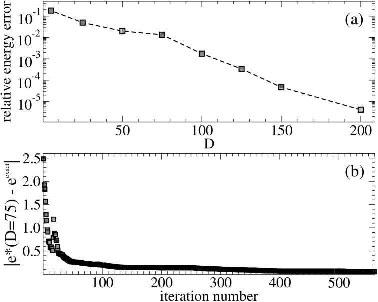
Figure 1: (a) The relative error, $|\frac{e^{*}(D)-\mathfrak{e}^{\rm exact}}{\mathfrak{e}^{\rm exact}}|$, in calculating the ground-state energies per site of $H_{XX}$, Eq. (4), from the proposed interior-point iMPS algorithm, $\mathfrak{e}^{*}(D)$, and the exact lower energy-per-site bound, $\mathfrak{e}^{\rm exact}=-4$, based on the argument presented in the text. Error bars are smaller than the symbol size and the dashed line is provided only as a guide for the eye. (b) The iMPS ground state energies for $H_{XX}$ versus iteration number for a selected series of interior point calculations with $D=75$ (notice each iteration of the interior-point algorithm itself typically contains hundreds of function evaluations).

The energies per site, $\mathfrak{e}^{*}$, for the optimized interior-point iMPS ground states of $H_{XX}$ and selected bond dimensions are presented in Fig. (1)(a). There, we report the energy difference with respect to a reference/benchmark ground-state energy per site, $\mathfrak{e}^{\rm exact}=-4$, which we argue is achievable (e.g. through an iMPS representation with $D\rightarrow\infty$) and analytically show in the following that is an exact lower bound on the energies of the Hamiltonian (Saadatmand and McCulloch, 2019). The Hamiltonian can be written as $H_{XX}=(\hat{S}^{+}_{\rm total}\hat{S}^{-}_{\rm total}+\text{h.c.})-\sum_{i}(\hat{S}^{+}_{i}\hat{S}^{-}_{i}+\text{h.c.})$. The first term in this form is completely positive and its expectation value is lower bounded by zero. Therefore, if we find the state that maximizes the expectation value of $\sum_{i}(\hat{S}^{+}_{i}\hat{S}^{-}_{i})$ and essentially satisfies $\hat{S}^{+}_{\rm total}\ket{\text{ground}}=0$ and $\hat{S}^{-}_{\rm total}\ket{\text{ground}}=0$, in principle, it would set the lower bound on the energy per site of $H_{XX}$. Consequently, the true paramagnetic ground state can be perturbatively (ignoring the normalization) written as

$$\ket{\text{ground}}_{\rm exact}\propto \ket{\cdots,0,0,0,\cdots}+$$

$$\sum_{\rm permut.~{}of~{}\pm 1~{}and~{}0s} \ket{\cdots,0,1,\cdots,0,\cdots,-1,0,\cdots}+$$

$$\sum_{\rm permut.~{}of~{}\pm 1~{}and~{}0s} \ket{\cdots,0,1,1,\cdots,0,\cdots,-1,-1,0,\cdots}$$

$$+\cdots,$$ (15)

which guarantees that the expectation values of $\hat{S}^{+}_{\rm total}$ and $\hat{S}^{-}_{\rm total}$ vanish and leads to maximum energy per site value of $4$ for the expectation value of $\sum_{i}(\hat{S}^{+}_{i}\hat{S}^{-}_{i}+\text{h.c.})$ for spin-$1$ particles.

It is clear from Fig. (1)(a) that the iMPS wave function’s energy per site consistently decreases toward the true ground state as $D$ increases as desired. (We have also empirically confirmed that the correlation functions of type $\langle\hat{S}^{+}_{r}\hat{S}^{-}_{0}\rangle$ decay, indeed, exponentially with $r$ as it is expected from such iMPS ground states.) In addition, Fig. (1)(b) demonstrates that such interior-point iMPS optimization is, after doing enough number of initial iterations, systematically converging toward a true energy minimum as more iterations are performed for this exemplary series of calculations with $D\!=\!75$. We argue these results provide strong support for the effectiveness and functionality of the interior-point iMPS algorithm. (Let us also note that some patterns in the structure of the $A$-matrices’ elements may be physically irrelevant in practice; in particular, while the ratios between magnitudes is physically important, some other values have been observed to become insignificantly small due to the fact that the algorithm has to stop after some finite number of iterations (Baker et al., ).)

In the end, we briefly review the physical consequences of the results in Fig. (1)(a). The fact that the iMPS is converging closer and closer to the analytical state in Eq. (15) with energy $\mathfrak{e}^{\rm exact}$ , which corroborates that the perturbatively presented wave function is indeed the true ground state. Now, it can be also easily verified (using a similar argument as above) that the ground states of one-dimensional global-range antiferromagnetic XX Heisenberg models, as in Eq. (4), with $J>0$ and few sites are some paramagnets having superpositions of permuting $\{-1,0,1\}$ patterns. In fact, here, we analytically and numerically established that for the infinite-range case of Eq. (4) the true ground state is again a similar paramagnet possessing the specific permuting patterns shown in Eq. (15). This is while, in a distinct way, the paramagnetic phase of the nearest-neighbor XX model lives on a critical XY-Haldane point of XYZ Heisenberg Hamiltonian with no infinite-order phase transition Malvezzi et al. (2016). Our results provide a framework for future works to study infinite-dimensional variants of XYZ Hamiltonian to investigate possible existence/absence of Kosterlitz-Thouless-type transitions.

VI Conclusion

We have presented an efficient iterative tensor network approach to systematically find the ground states of infinite-dimensional spin Hamiltonians based on explicit constrained optimizations of their iMPS description. We exemplified how to greatly reduce the number of free parameters in the optimizations by employing built-in symmetries for the iMPS ansatz. Previously, the phase diagram of such Hamiltonians have been only studied in the thermodynamic limit for a number of exactly-solvable cases to our knowledge. We therefore offered a new tensor network algorithm specialized for scrutinizing extreme non-locality of infinite-size systems exhibiting infinite-range interactions.

The presented algorithm sits next to the slightly more efficient generic tensor-network solvers of iDMRG and VUMPS, which can be employed to find ground states of non-decaying Hamiltonians in the thermodynamic limit as well. In other words, our results demonstrate that one can also derive such ground states by directly optimizing iMPS operators’ elements, while relying on no density matrix truncation and extra explicit orthogonalization steps (as also previously claimed in Ref. (Östlund and Rommer, 1995)); this could offer a simpler structure for implementation of the symmetry constraints and usefulness for pedagogical purposes. We expect that the phase diagrams of a wide range of infinite-range models of experimental or foundational importance (most notably variants of quantum Dicke-Bose-Hubbard-type models as in cavity-mediated bosonic experiments and infinite-dimensional XYZ Heisenberg Hamiltonians) can be now elucidated using interior-point iMPS to guide the direction of the future experiments.

Perhaps, the main physical application for the presented algorithm is to provide an optimization approach for infinite-dimensional effective Heisenberg Hamiltonians emulating idealistic multi-mode laser models (Baker et al., ): in these systems, the symmetry constraints finds complicated algebraic forms (in comparison to, e.g., $\{A^{[j]}_{m,n}\neq 0~{}\text{iff}~{}m+j=n\}$ used above) and may become incompatible with existing symmetric iDMRG and VUMPS routines. Nevertheless, the brute-force interior-point iMPS can always handle closed forms of symmetry equations as built-in nonlinear constraints.