MLAT: Metric Learning for kNN in Streaming Time Series

Abstract.

Learning a good distance measure for distance-based classification in time series leads to significant performance improvement in many tasks. Specifically, it is critical to effectively deal with variations and temporal dependencies in time series. However, existing metric learning approaches focus on tackling variations mainly using a strict alignment of two sequences, thereby being not able to capture temporal dependencies. To overcome this limitation, we propose MLAT, which covers both alignment and temporal dependencies at the same time. MLAT achieves the alignment effect as well as preserves temporal dependencies by augmenting a given time series using a sliding window. Furthermore, MLAT employs time-invariant metric learning to derive the most appropriate distance measure from the augmented samples which can also capture the temporal dependencies among them well. We show that MLAT outperforms other existing algorithms in the extensive experiments on various real-world data sets.

1. Introduction

Streaming time series classifications play an increasingly important role in activity recognition (Mueen and Keogh, 2016) and fraud detection (Junqué de Fortuny et al., 2014). However, since the number of labels in streaming time series data is often insufficient to build a high-quality classifier (Wei and Keogh, 2006), $k$-nearest neighbor (kNN), a non-parametric method, is widely used and it empirically results in high accuracy in several applications (Ding et al., 2008).

In accordance with this trend, many studies have been focused on improving the performance of kNN by designing more appropriate distance measures for a given data set. Recently, various time series metric learning approaches (Mei et al., 2016; Shen et al., 2017; Che et al., 2017) have been developed to achieve this goal. Because variations in time series data, such as sequence shifting and scaling, is one of the main challenges, the existing algorithms consist of the two phases: (i) alignment and (ii) metric learning. As shown in Figure 1(a), the subsequences of the time series data are aligned in pairs to match the optimal time steps (dotted line), rendering them robust to variation. Metric learning is subsequently conducted on the local distance $D_{l}$ computed from the matched time steps, which minimizes the distance of pairs with the same label and maximizes for pairs with different labels.

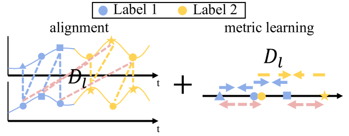
(a) Metric learning on local distances.

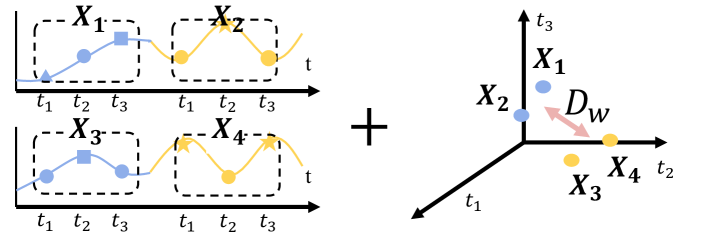
(b) Metric learning on window distances.

Figure 1. The effect of alignment to temporal dependency.

However, since the local distance only considers the difference between features at a single matched time step, metric learning on the local distance does not capture temporal dependencies appearing across consecutive time steps. Temporal dependency is known to greatly enhance the performance of time series classifications (Hochreiter and Schmidhuber, 1997). For example, when we try to distinguish between forwards and backwards from a set of motion images of a walking person, an image of a single time step gives very limited information on the direction, whereas a set of images of consecutive time steps provides clear clues. It is, therefore, more effective to distinguish samples with different labels by applying metric learning on the window distance $D_{w}$ computed from consecutive time steps (e.g., $\{t_{1},t_{2},t_{3}\}$), as shown in Figure 1(b). The existing algorithms miss out this opportunity as they focus on alignment at the expense of the temporal dependencies. This calls for a new method that can achieve both alignment and temporal dependencies.

In this paper, we propose a novel metric learning algorithm for kNN in streaming time series, called MLAT (Metric Learning considering Alignment and Temporal dependencies). To account for both alignment and temporal dependency in learning a distance measure, MLAT consists of the two main phases:

1. Sliding Window Augmentation: MLAT augments a given time series using sliding window sampling (Ye and Keogh, 2009) to achieve the alignment effect while preserving the temporal dependencies. As shown in Figure 2, by extracting all possible samples as sets of consecutive time steps with a fixed length, the samples having similar patterns can be well-aligned even without explicit time step matching. At the same time, because consecutive time steps are well preserved in a sample, MLAT can exploit the temporal dependencies between them.

2. Time-Invariant Metric Learning: The temporal dependencies between features of augmented samples are time-invariant, meaning that the dependency of two features in a fixed time difference is consistent regardless of their absolute temporal locations; i.e., the dependency of two features at time $t$ and $t+1$ is equal to that of the two features at time $t+1$ and $t+2$. Thus, MLAT tries to fulfill this inherent characteristic in learning distance metric using the large margin nearest neighbor (LMNN) (Lu et al., 2015), constraining a Mahalanobis matrix to be a Block Toeplitz (Gray et al., 2006) structure.

Extensive experiments on four real-world streaming time series data sets indicate that MLAT results in promising kNN performance.

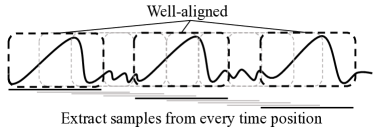
Figure 2. Sliding window augmentation.

2. Related Work

We briefly review several existing studies to find better distance measures in time series data with respect to the following aspects: (i) alignment to appropriately handle variation, and (ii) metric learning to learn a better distance function.

2.1. Alignment

Dynamic time warping (DTW) (Berndt and Clifford, 1994) is the most represensatice method to match the time steps of two samples in order to find the best warping path. Numerous variants of DTW have been studied, whose focus is on resolving the inefficiencies in time step matching (Mueen and Keogh, 2016; Rakthanmanon et al., 2012) and the invalidity of the triangle inequality in the learned distance (Cuturi et al., 2007; Hogeweg and Hesper, 1984). However, DTW-based alignment methods fail to deal with the temporal dependencies because they explicitly match the time steps.

2.2. Metric Learning

Most time series metric learning algorithms in the literature apply metric learning to the local distance computed using DTW based alignment. LDML-DTW (Mei et al., 2016) and LMNN-DTW (Shen et al., 2017) first match time steps by multivariate dynamic time warping (MDTW) (Berndt and Clifford, 1994), and subsequently learn the Mahalanobis matrix of the local distance using LogDet divergence and Large Margin Nearest Neighbor (LMNN) (Weinberger and Saul, 2009), respectively. DECADE (Che et al., 2017) devised a new alignment method to learn the valid distance measure while using deep networks to capture the complex dependencies in the local distance. There have been a few studies for learning the distance representation in the embedded space obtained from the last hidden layer of LSTM (Mueller and Thyagarajan, 2016). However, to the best of our knowledge, no studies yet simultaneously consider alignment and temporal dependencies in time series metric learning.

3. Preliminary

3.1. Problem Setting

We introduce the main concepts in the kNN classification problem on streaming time series in the following definitions, as also illustrated in Figure 3.

Definition 3.1.

(Streaming time series) A multivariate streaming time series $x=[x_{1},x_{2},\cdots,x_{\mathbb{T}}]$ is a sequential observation of $x_{i}\in\mathbb{R}^{d}$ with $d$ features, where $\mathbb{T}$ is the length of $x$.

Definition 3.2.

(State) A state $s_{j}\in\{1,2,\cdots,S\}$ denotes the label of a sequence in a time series $x$ during the time period $T_{j}\,(\subset\mathbb{T})$, where $S$ is the number of states in $x$ and $j$ is the index of the state. The time series $x$ consists of various sizes of sequences with different states; for example, a time series $x$ collected from wearable devices for $15$ min consists of the two sequences: a ”walk” state of the first $10$ min and a ”run” state of the last $5$ min.

Definition 3.3.

(Sample) A sample $X_{t}=[x_{t},\cdots,x_{t+w-1}]\in\mathbb{R}^{d\times w}$ is a subsequence of size $w$ extracted from a certain sequence in time period $T_{j}$ of a time series $x$. It consists of the consecutive time steps from time $t$ to time $t+w-1$. The state $s_{j}$ of the sequence becomes the label $y_{t}$ of $X_{t}$.

Definition 3.4.

(kNN classification problem) Let $\mathbb{D}$ be a set of samples from a time series $x$. The kNN classification problem in streaming time series classifies the label of a sample $X_{new}$ by referring to that of the k nearest neighbors of $X_{new}$ in $\mathbb{D}$.

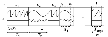
Figure 3. Stream kNN settings.

3.2. Large Margin Nearest Neighbor (Weinberger and Saul, 2009)

Most metric learning methods aim at learning a Mahalanobis distance matrix $\mathbf{M}$ (Weinberger and Saul, 2009; Davis et al., 2007), where the distance is defined as:

(1) $$\small D_{\mathbf{M}}(X_{i},X_{j})=(X_{i}-X_{j})^{T}\mathbf{M}(X_{i}-X_{j}),$$

where $X_{i}$ and $X_{j}\in\mathbb{R}^{dw}$ are two samples and $\mathbf{M}\in\mathbb{R}^{dw\times dw}$ is a positive semidefinite matrix. Given a set of samples $\mathbb{D}$, for each sample $X_{i}\in\mathbb{D}$, LMNN first finds the $k$ nearest neighbors of $X_{i}$ based on the Euclidean distance and calls them target neighbors. Subsequently, LMNN learns the optimal Mahalanobis distance matrix $\mathbf{M}$ which minimizes the following loss function:

(2) $$\small\begin{split}\underset{\mathbf{M}\succeq 0}{\min}\ &\mathcal{E}^{lmnn}(\mathbf{M})=(1-c)\sum_{ij}\eta_{ij}{D_{\mathbf{M}}}(X_{i},X_{j})\\ &+c\sum_{ijl}\eta_{ij}(1-y_{il})\left[1+D_{\mathbf{M}}(X_{i},X_{j})+D_{\mathbf{M}}(X_{i},X_{l})\right]_{+},\end{split}$$

where $c\in[0,1]$ controls the weights of the two penalizing terms, $\eta_{ij}\in\{0,1\}$ indicates whether $X_{j}$ is a target neighbor of $X_{i}$, $y_{il}\in\{0,1\}$ indicates whether $X_{i}$ and $X_{l}$ have the same label or not. Here, the first term penalizes the large distance from each sample to its $k$ target neighbors, and the second term penalizes the small distance from each sample to all other samples that do not share the same label.

4. Methodology

MLAT consists of two phases: (1) Sliding window augmentation, and (2) Time-invariant metric learning. Algorithm 1 describes the overall procedure of MLAT.

4.1. Phase I: Sliding Window Augmentation

Phase I enables metric learning to consider alignment and temporal dependencies concurrently. Specifically, all possible samples in $x$ can be extracted by sliding a fixed sized window from the beginning of $x$. Some parts of $x$ where the state switches are exempted from the augmentation. These augmented samples become the training set for metric learning and help to achieve the alignment effect. As in Figure 4(a), a sample $X$ has the most well-aligned training sample $X_{target(i)}$ as its neighbor with euclidean distance. Therefore, MLAT, which is based on LMNN, exploits the well-aligned samples $X_{target(i)}$ as the target neighbor of $X$ if they share the same label and consequently learns the distance that makes them close as in Figure 4(b). Temporal dependencies can also be considered because metric learning is applied on window distance ($\mathbf{M}\in\mathbb{R}^{dw\times dw}$).

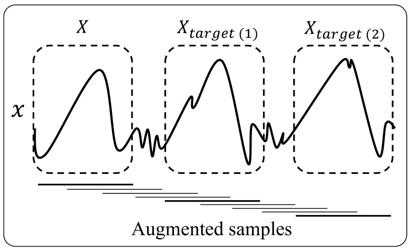
(a) Phase I.

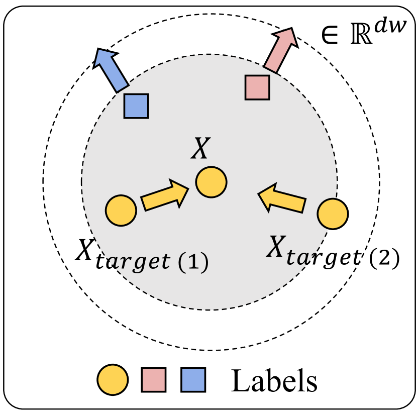
(b) Phase II.

Figure 4. Overall procedure of MLAT.

Algorithm 1 MLAT

0:  A multivariate streaming time series $x$;

0:  The optimal Mahalanobis matrix $M$;

1:  /* Phase I: sliding window augmentation */

2:  $X\leftarrow$ Extract augmented samples from $x$;

3:  /* Phase II: time-invariant metric learning */

4:  $\mathbf{L}\leftarrow I,\mathbf{M}^{0}\leftarrow I,\mathbf{Z}^{0}\leftarrow 0,\mathbf{U}^{0}\leftarrow 0$; /* Initialize parameters. */

5:   for $k=1,2,\cdots,K$ (until convergence) do /* Update parameters. */

6:       repeat

7:          Calculate $\bigtriangledown\mathbf{M}^{k+1}\leftarrow{\partial\mathcal{E}^{lmnn}/\partial\mathbf{M}^{k+1}}+\rho(\mathbf{M}^{k+1}-\mathbf{Z}^{k}+\mathbf{U}^{k})$;

8:          Calculate $\bigtriangledown\mathbf{L}\leftarrow 2\mathbf{L}\times{\bigtriangledown\mathbf{M}^{k+1}}$;

9:          Update $\mathbf{L}\leftarrow(\mathbf{L}-\alpha\bigtriangledown\mathbf{L})$ and $\mathbf{M}^{k+1}\leftarrow\mathbf{L}^{T}\mathbf{L}$;

10:       until Converge;

11:       $\mathbf{Z}^{k+1}_{B^{(m)}_{ij}}\leftarrow\sum_{l=1}^{R^{(m)}}{(\mathbf{M}^{k+1}+\mathbf{U}^{k})_{B^{(m)}_{ij,l}}/{R^{(m)}}}$;

12:       $\mathbf{U}^{k+1}\leftarrow\mathbf{U}^{k}+(\mathbf{M}^{k+1}-\mathbf{Z}^{k+1})$;

13:  return  $\mathbf{M}^{K}$;

4.2. Phase II: Time-Invariant Metric Learning

Phase II allows metric learning to capture the time-invariant property of the augmented samples, making it more effective for kNN.

4.2.1. Block Toeplitz

As a result of Phase I, the consecutive samples are mostly overlapped. This leads to the covariance matrix of augmented samples in the form of Block Toeplitz (Gray et al., 2006) as stated in Definition 4.1, which is proven by Theorem 4.2.

Definition 4.1.

(Block toeplitz (Gray et al., 2006)) A $dw\times dw$ block toeplitz matrix $\mathbf{A}$ with $d\times d$ sub-blocks $\mathbf{A}^{(m)}$ has the following form:

(3) $$\small\begin{split}\mathbf{A}&=\begin{bmatrix}\mathbf{A}^{(0)}&(\mathbf{A}^{(1)})^{T}&(\mathbf{A}^{(2)})^{T}&\cdots&(\mathbf{A}^{(w-1)})^{T}\\ \mathbf{A}^{(1)}&\mathbf{A}^{(0)}&(\mathbf{A}^{(1)})^{T}&\ddots&\vdots\\ \mathbf{A}^{(2)}&\mathbf{A}^{(1)}&\ddots&(\mathbf{A}^{(1)})^{T}&(\mathbf{A}^{(2)})^{T}\\ \vdots&\ddots&\mathbf{A}^{(1)}&\mathbf{A}^{(0)}&(\mathbf{A}^{(1)})^{T}\\ \mathbf{A}^{(w-1)}&\cdots&\mathbf{A}^{(2)}&\mathbf{A}^{(1)}&\mathbf{A}^{(0)}\\ \end{bmatrix}\ ,\end{split}$$

where the sub-block $\mathbf{A}^{(m)}$ appears $w-m$ times in $\mathbf{A}$ and has the same value at all occurrences.

Theorem 4.2.

Let $\mathbb{D}_{s}=[X_{1},X_{2},\cdots,X_{L}]\in\mathbb{R}^{dw\times L}$ be a set of samples obtained by sliding window augmentation, where $X_{t}\in\mathbb{R}^{dw}$ and $L\gg w$. The covariance matrix $\boldsymbol{\Sigma}\in\mathbb{R}^{dw\times dw}$ of $\mathbb{D}_{s}$ is in the form of Block Toeplitz.

Proof.

$\mathbb{D}_{s}$ is represented with $w$ row partitions as follows:

(4) $$\small\begin{split}\mathbb{D}_{s}&=\begin{bmatrix}x_{1}&x_{2}&x_{3}&\cdots&x_{L-w+1}\\ x_{2}&x_{3}&x_{4}&\cdots&x_{L-w+2}\\ \vdots&\vdots&\vdots&&\vdots\\ x_{w}&x_{w+1}&x_{w+2}&\cdots&x_{L}\\ \end{bmatrix}\ ,\end{split}$$

where $x_{i}\in\mathbb{R}^{d}$. Since most portions in each row partition overlap, the mean $\mu_{p}\in\mathbb{R}^{d}$ of each row partition is approximately the same. Then, by the definition of the covariance matrix, $\boldsymbol{\Sigma}=1/L\cdot(\mathbb{D}_{s}-\mu)(\mathbb{D}_{s}-\mu)^{T}$ approximately takes Block Toeplitz form, where $\mu=[\mu_{p},\cdots,\mu_{p}]^{T}\cdot 1_{L}^{T}\in\mathbb{R}^{dw\times L}$. ∎

The $(i,j)$-th element of the covariance matrix corresponds to the dependency between the $i$-th and $j$-th features, and if the matrix is Block Toeplitz, the dependency between the two features is time-invariant (Hallac et al., 2017). Note that the time-invariant dependencies of the augmented samples should be preserved when learning distance.

4.2.2. Time-Invariant Constraints

Here, we first analyze how the Mahalanobis matrix handles the dependency between two features. Eq. (1) can be represented as follows:

(5) $$\small\begin{split}D_{\mathbf{M}}(X_{i},X_{j})&=tr(\mathbf{M}(X_{1}-X_{2})^{T}(X_{1}-X_{2}))\\ &=\sum_{ij}\mathbf{M}_{ij}(X_{1}^{(i)}-X_{2}^{(i)})(X_{1}^{(j)}-X_{2}^{(j)}),\end{split}$$

where $X_{1}^{(i)},i\in\{1,\cdots,dw\}$, is the $i$-th feature scala value of a sample $X_{1}$, and $\mathbf{M}_{ij}$ is the $(i,j)$-th element of $\mathbf{M}$. $\mathbf{M}_{ij}$ decides how much the product of the distance between $i$-th features and that of $j$-th features affects the total distance, meaning that $\mathbf{M}_{ij}$ handles the dependency between the $i$-th and $j$-th features.

To preserve the time-invariant dependencies, we propose the following time-invariant metric learning framework:

(6) $$\small\begin{split}\underset{\mathbf{M}}{\min}\quad\mathcal{E}^{lmnn}(\mathbf{M})\quad\qquad\\ \rm{\text{subject to}}:\ \mathbf{M}\succeq 0,\ \mathbf{M}\in\mathcal{T},\end{split}$$

where $\mathcal{T}$ is a set of $dw\times dw$ symmetric Block Toeplitz matrices. By constraining $\mathbf{M}$ to be Block Toeplitz, the distances between two features in the same time difference should be regarded equally, with the same values as in $\mathbf{M}$. Thus, the optimal matrix can effectively capture the time-invariant dependencies structure.

4.2.3. Optimization

We solve the proposed optimization problem using the alternating direction method of multipliers (ADMM) (Boyd et al., 2011). We transform Eq. (6) into an ADMM-friendly form as follows:

(7) $$\small\begin{split}\mathcal{L}_{\rho}(\mathbf{M},&\mathbf{Z},\mathbf{U})=\mathcal{E}^{lmnn}(\mathbf{M})+{\rho\over 2}\parallel\mathbf{M}-\mathbf{Z}+\mathbf{U}\parallel_{F}^{2}\\ &\rm{\text{subject to}}:\mathbf{Z}\in\mathcal{T},\ \mathbf{Z}=\mathbf{M},\ \mathbf{M}\succeq 0.\end{split}$$

Then, the following three steps are repeated until convergence.

(8) $$\small\begin{split}(a)\ \mathbf{M}^{k+1}&=\underset{\mathbf{M}}{argmin}\ \mathcal{L}_{\rho}(\mathbf{M},\mathbf{Z}^{k},\mathbf{U}^{k})\\ (b)\ \mathbf{Z}^{k+1}&=\underset{\mathbf{Z}}{argmin}\ \mathcal{L}_{\rho}(\mathbf{M}^{k+1},\mathbf{Z},\mathbf{U}^{k})\\ (c)\ \mathbf{U}^{k+1}&=\mathbf{U}^{k}+(\mathbf{M}^{k+1}-\mathbf{Z}^{k+1}).\end{split}$$

$\mathbf{M}$-update: The $\mathbf{M}$-update can be written as:

(9) $$\small\begin{split}\mathbf{M}^{k+1}&=\underset{\mathbf{M}\succeq 0}{argmin}\ \mathcal{E}^{lmnn}(\mathbf{M})+{\rho\over 2}\parallel\mathbf{M}-\mathbf{Z^{k}}+\mathbf{U^{k}}\parallel_{F}^{2}.\end{split}$$

This problem can be solved by the gradient descent method. To ensure a positive semi-definite $\mathbf{M}$, MLAT factorizes $\mathbf{M}$ as $\mathbf{M}=\mathbf{L}^{T}\mathbf{L}$ and updates $\mathbf{L}$ through sub-gradient descent. Here, the sub-gradient of Eq. (9) with respect to $\mathbf{L}$ is ${\partial\mathcal{E}^{lmnn}\over\partial\mathbf{L}}=2\mathbf{L}({\partial\mathcal{E}^{lmnn}\over\partial\mathbf{M}}+\rho(\mathbf{M}-\mathbf{Z}^{k}+\mathbf{U}^{k}))$ by the chain rule.

$\mathbf{Z}$-update: The closed form solution of the $\mathbf{Z}$-update is as follows:

(10) $$\small\begin{split}\mathbf{Z}^{k+1}_{B^{(m)}_{ij}}&={\sum_{l=1}^{R^{(m)}}{(\mathbf{M}^{k+1}+\mathbf{U}^{k})_{B^{(m)}_{ij,l}}/{R^{(m)}}}},\end{split}$$

where $B^{(m)}_{ij,l}$ is the index $(x,y)$ at $\mathbf{Z}$ of the $(i,j)$-th element of the $l$-th occurrence sub-matrix $\mathbf{Z}^{(m)}$, and $R^{(m)}$ is the number of occurrences of $\mathbf{Z}^{(m)}$ in $\mathbf{Z}$. Refer to (Hallac et al., 2017) for details.

5. Experiments

To validate the superiority of MLAT, we performed the kNN classification task on four real-world streaming time series data sets. The experimental results confirmed that MLAT maintains its dominance over other algorithms.

5.1. Experiment Setup

5.1.1. Data Sets

Table 1. Summary statistics of the UCI dataset.

Data Set	Description	Dims	$\#$ Lables
SCMA (from Single Chest-Mounted Accelerometer (SCMA) Data Set, 2014)	3D wearable accelerometer sensors	3	7
AReM (system based on Multisensor data fusion (AReM) Data Set, 2016)	Wireless Sensor Network	6	6
EMG (Set, 2011a)	Eight Electromyogram(EMG) sensors	8	5
Vicon (Set, 2011b)	Nine Vicon 3D trackers	27	5

The statistics of the four benchmark data sets are summarized in Table 1. Note that we only used $5$ ambiguous labels defined as normal activities in EMG and Vicon data sets for a more difficult kNN task.

5.1.2. Algorithms

We compared MLAT with four existing algorithms for measuring distance in time series:

• ED : Euclidean distance (baseline).

• MDTW (Berndt and Clifford, 1994) : Multivariate dynamic time warping.

• LDMLT (Mei et al., 2016) : Learning local distance by DTW alignment.

• LMNN (Lu et al., 2015) : Large Margin Nearest Neighbor.

• MLAT : Our proposed method.

5.1.3. Settings

We assumed that $510$ consecutive observations ($|T_{j}|$ = $510$) from each label are given for each data set, except AReM where $|T_{j}|$ is $480$. The training samples, where the size $w$ is set to 10, were extracted from the given observations. For existing algorithms, we randomly extracted 100 samples from each label. We set $k$ to 1 for kNN because 1-NN is widely accepted as the most accurate for many tasks (Ding et al., 2008). We randomly selected the starting time of the consecutive observations and reported the average results of the five experiments for each dataset.

5.2. Experimental Results

Table 2. Accuracy (%) of kNN with standard deviation ($k=1$).

Data Set	ED	DTW	LDMLT	LMNN	MLAT
SCMA	97.5$\pm$0.6	98.5$\pm$0.5	97.4$\pm$0.5	99.1$\pm$0.4	99.5$\pm$0.1
AReM	75.3$\pm$1.2	76.4$\pm$1.9	84.4$\pm$2.1	73.3$\pm$1.5	80.8$\pm$0.8
EMG	61.8$\pm$2.3	65.4$\pm$1.5	65.2$\pm$2.8	65.9$\pm$2.1	69.3$\pm$1.7
Vicon	73.3$\pm$1.9	75.8$\pm$2.1	72.2$\pm$3.3	81.5$\pm$2.6	84.9$\pm$1.8

5.2.1. Overall Accuracy

Table 2 shows the kNN accuracy of the five algorithms. In the SCMA, EMG, and Vicon data sets, MLAT achieved the highest accuracy compared with other algorithms. LDMLT produced the highest accuracy for the AReM data set, but MLAT also achieved a significant improvement compared with the remaining algorithms. This emphasizes the need to consider both alignment and temporal dependencies.

Table 3. Accuracy improvement (%) on augmented samples.

Data Set	ED	DTW	LDMLT	LMNN
SCMA	1.02	0.40	1.33	0.20
AReM	-0.21	0.52	1.30	0.41
EMG	5.34	3.52	-1.4	2.43
Vicon	3.27	-0.13	-2.2	2.33

5.2.2. Effect of Phases I and II

All the existing algorithms were also evaluated on augmented samples obtained in Phase I. As shown in Table 3, the accuracy of the algorithms were significantly improved by up to $5.3\%$ compared with the accuracy from randomly extracted samples. This shows that augmenting well-aligned samples is evidently beneficial for the time series classification.

In addition, MLAT still outperformed LMNN by up to $9.8\%$, though LMNN performed on augmented samples. The performance of metric learning for time series can thus be further boosted by preserving the time-invariant characteristic.

6. Conclusion

In this paper, we proposed MLAT, a novel metric learning algorithm that considers the two main characteristics in time series, i.e., variation and temporal dependencies, by using sliding window augmentation and time-invariant metric learning, respectively. Using four real-world data sets, we showed that MLAT outperforms the existing algorithms in most cases. For future work, we will tackle more challenging settings where more complex variations and temporal dependencies exist.

- (1)
- Berndt and Clifford (1994) Donald J Berndt and James Clifford. 1994. Using dynamic time warping to find patterns in time series.. In KDD workshop, Vol. 10. Seattle, WA, 359–370.
- Boyd et al. (2011) Stephen Boyd, Neal Parikh, Eric Chu, Borja Peleato, Jonathan Eckstein, et al. 2011. Distributed optimization and statistical learning via the alternating direction method of multipliers. Foundations and Trends® in Machine learning 3, 1 (2011), 1–122.
- Che et al. (2017) Zhengping Che, Xinran He, Ke Xu, and Yan Liu. 2017. DECADE: a deep metric learning model for multivariate time series. In KDD workshop on mining and learning from time series.
- Cuturi et al. (2007) Marco Cuturi, Jean-Philippe Vert, Oystein Birkenes, and Tomoko Matsui. 2007. A kernel for time series based on global alignments. In 2007 IEEE International Conference on Acoustics, Speech and Signal Processing-ICASSP’07, Vol. 2. IEEE, II–413.
- Davis et al. (2007) Jason V Davis, Brian Kulis, Prateek Jain, Suvrit Sra, and Inderjit S Dhillon. 2007. Information-theoretic metric learning. In Proceedings of the 24th international conference on Machine learning. ACM, 209–216.
- Ding et al. (2008) Hui Ding, Goce Trajcevski, Peter Scheuermann, Xiaoyue Wang, and Eamonn Keogh. 2008. Querying and mining of time series data: experimental comparison of representations and distance measures. Proceedings of the VLDB Endowment 1, 2 (2008), 1542–1552.
- from Single Chest-Mounted Accelerometer (SCMA) Data Set (2014) Activity Recognition from Single Chest-Mounted Accelerometer (SCMA) Data Set. 2014. https://archive.ics.uci.edu/ml/datasets/Activity+Recognition+from+Single+Chest-Mounted+Accelerometer. Accessed: 2019-03-01.
- Gray et al. (2006) Robert M Gray et al. 2006. Toeplitz and circulant matrices: A review. Foundations and Trends® in Communications and Information Theory 2, 3 (2006), 155–239.
- Hallac et al. (2017) David Hallac, Sagar Vare, Stephen Boyd, and Jure Leskovec. 2017. Toeplitz inverse covariance-based clustering of multivariate time series data. In Proceedings of the 23rd ACM SIGKDD International Conference on Knowledge Discovery and Data Mining. ACM, 215–223.
- Hochreiter and Schmidhuber (1997) Sepp Hochreiter and Jürgen Schmidhuber. 1997. Long short-term memory. Neural computation 9, 8 (1997), 1735–1780.
- Hogeweg and Hesper (1984) Paulien Hogeweg and Ben Hesper. 1984. The alignment of sets of sequences and the construction of phyletic trees: an integrated method. Journal of molecular evolution 20, 2 (1984), 175–186.
- Junqué de Fortuny et al. (2014) Enric Junqué de Fortuny, Marija Stankova, Julie Moeyersoms, Bart Minnaert, Foster Provost, and David Martens. 2014. Corporate residence fraud detection. In Proceedings of the 20th ACM SIGKDD international conference on Knowledge discovery and data mining. ACM, 1650–1659.
- Lu et al. (2015) Jiwen Lu, Gang Wang, Weihong Deng, and Kui Jia. 2015. Reconstruction-based metric learning for unconstrained face verification. IEEE Transactions on Information Forensics and Security 10, 1 (2015), 79–89.
- Mei et al. (2016) Jiangyuan Mei, Meizhu Liu, Yuan-Fang Wang, and Huijun Gao. 2016. Learning a mahalanobis distance-based dynamic time warping measure for multivariate time series classification. IEEE transactions on Cybernetics 46, 6 (2016), 1363–1374.
- Mueen and Keogh (2016) Abdullah Mueen and Eamonn Keogh. 2016. Extracting optimal performance from dynamic time warping. In Proceedings of the 22nd ACM SIGKDD International Conference on Knowledge Discovery and Data Mining. ACM, 2129–2130.
- Mueller and Thyagarajan (2016) Jonas Mueller and Aditya Thyagarajan. 2016. Siamese recurrent architectures for learning sentence similarity. In Thirtieth AAAI Conference on Artificial Intelligence.
- Rakthanmanon et al. (2012) Thanawin Rakthanmanon, Bilson Campana, Abdullah Mueen, Gustavo Batista, Brandon Westover, Qiang Zhu, Jesin Zakaria, and Eamonn Keogh. 2012. Searching and mining trillions of time series subsequences under dynamic time warping. In Proceedings of the 18th ACM SIGKDD international conference on Knowledge discovery and data mining. ACM, 262–270.
- Set (2011a) EMG Physical Action Data Set Data Set. 2011a. https://archive.ics.uci.edu/ml/datasets/EMG+Physical+Action+Data+Set. Accessed: 2019-03-01.
- Set (2011b) Vicon Physical Action Data Set Data Set. 2011b. https://archive.ics.uci.edu/ml/datasets/Vicon+Physical+Action+Data+Set. Accessed: 2019-03-01.
- Shen et al. (2017) Jingyi Shen, Weiping Huang, Dongyang Zhu, and Jun Liang. 2017. A novel similarity measure model for multivariate time series based on LMNN and DTW. Neural Processing Letters 45, 3 (2017), 925–937.
- system based on Multisensor data fusion (AReM) Data Set (2016) Activity Recognition system based on Multisensor data fusion (AReM) Data Set. 2016. https://archive.ics.uci.edu/ml/datasets/Activity+Recognition+system+based+on+Multisensor+data+fusion+(AReM). Accessed: 2019-03-01.
- Wei and Keogh (2006) Li Wei and Eamonn Keogh. 2006. Semi-supervised time series classification. In Proceedings of the 12th ACM SIGKDD international conference on Knowledge discovery and data mining. ACM, 748–753.
- Weinberger and Saul (2009) Kilian Q Weinberger and Lawrence K Saul. 2009. Distance metric learning for large margin nearest neighbor classification. Journal of Machine Learning Research 10, Feb (2009), 207–244.
- Ye and Keogh (2009) Lexiang Ye and Eamonn Keogh. 2009. Time series shapelets: a new primitive for data mining. In Proceedings of the 15th ACM SIGKDD international conference on Knowledge discovery and data mining. ACM, 947–956.