Renormalization and Matching for the Collins-Soper Kernel from Lattice QCD

Abstract

The Collins-Soper kernel, which governs the energy evolution of transverse-momentum dependent parton distribution functions (TMDPDFs), is required to accurately predict Drell-Yan like processes at small transverse momentum, and is a key ingredient for extracting TMDPDFs from experiment. Earlier we proposed a method to calculate this kernel from ratios of the so-called quasi-TMDPDFs determined with lattice QCD, which are defined as hadronic matrix elements of staple-shaped Euclidean Wilson line operators. Here we provide the one-loop renormalization of these operators in a regularization-independent momentum subtraction (RI^′/MOM) scheme, as well as the conversion factor from the RI^′/MOM-renormalized quasi-TMDPDF to the $\overline{\rm MS}$ scheme. We also propose a procedure for calculating the Collins-Soper kernel directly from position space correlators, which simplifies the lattice determination.

1 Introduction

Transverse-momentum dependent parton distribution functions (TMDPDFs) describe the longitudinal and transverse momentum distribution of quarks and gluons in hadrons and nuclei, and thus are of vital interest to improving our understanding of hadronic and nuclear structure Boer:2011fh ; Accardi:2012qut . They are also crucial to predicting transverse momentum distributions in the Drell-Yan process, a key observable both for the Tevatron Affolder:1999jh ; Abbott:1999yd ; Abazov:2007ac ; Abazov:2010kn and the LHC Aad:2011gj ; Chatrchyan:2011wt ; Aad:2014xaa ; Khachatryan:2015oaa ; Aad:2015auj ; Khachatryan:2016nbe , as well as in semi-inclusive deep-inelastic scattering at low energies Ashman:1991cj ; Derrick:1995xg ; Adloff:1996dy ; Aaron:2008ad ; Airapetian:2012ki ; Adolph:2013stb ; Aghasyan:2017ctw .

TMDPDFs measure the transverse momentum $q_{T}$ carried by the struck parton. For perturbative $q_{T}\gg\Lambda_{\mathrm{QCD}}$, they can be calculated in terms of collinear parton distribution functions, and the resulting matching formula is known to next-to-next-to-leading order (NNLO) Catani:2011kr ; Catani:2012qa ; Gehrmann:2014yya ; Luebbert:2016itl ; Echevarria:2015byo ; Echevarria:2016scs ; Luo:2019hmp ; Luo:2019bmw . In contrast, for nonperturbative $q_{T}\lesssim\Lambda_{\mathrm{QCD}}$, TMDPDFs become genuinely nonperturbative objects which so far have only been extracted from measurements by performing global fits to a variety of experimental data sets, see e.g. refs. Landry:1999an ; Landry:2002ix ; Konychev:2005iy ; DAlesio:2014mrz ; Bacchetta:2017gcc ; Scimemi:2017etj . Since there are some issues associated to these extractions, in particular with reconciling low and high energy data, an independent determination from first principles is highly desirable. This has motivated studies with lattice QCD that have been carried out in refs. Musch:2010ka ; Musch:2011er ; Engelhardt:2015xja ; Yoon:2016dyh ; Yoon:2017qzo , primarily for ratios of moments in the longitudinal momentum fraction.

The TMDPDF $f_{i}(x,\vec{b}_{T},\mu,\zeta)$ for a parton of flavor $i$ depends on the longitudinal momentum fraction $x$ and the position space parameter $\vec{b}_{T}$, which is Fourier-conjugate to $\vec{q}_{T}$, as well as the renormalization scale $\mu$ and the Collins-Soper scale $\zeta$ Collins:1981va ; Collins:1981uk . The latter encodes the energy dependence of the TMDPDF, i.e. the momentum of the hadron or equivalently the hard scale of the scattering process, and the associated evolution is governed by the Collins-Soper equation Collins:1981va ; Collins:1981uk

$$\zeta\frac{\mathrm{d}}{\mathrm{d}\zeta}f_{i}(x,\vec{b}_{T},\mu,\zeta) =\frac{1}{2}\gamma^{i}_{\zeta}(\mu,b_{T})f_{i}(x,\vec{b}_{T},\mu,\zeta)\,.$$ (1)

The $\gamma^{i}_{\zeta}(\mu,b_{T})$ that appears here is referred to as either the Collins-Soper (CS) kernel or rapidity anomalous dimension for the TMDPDF. From consistency of the $\zeta$ and $\mu$ evolution equations, combined with information on the all order structure of the renormalization for Wilson line operators, it is known to have the all-order structure

$$\gamma_{\zeta}^{i}(\mu,b_{T})=-2\int_{1/b_{T}}^{\mu}\frac{\mathrm{d}\mu^{\prime}}{\mu^{\prime}}\Gamma_{\rm cusp}^{i}[\alpha_{s}(\mu^{\prime})]+\gamma_{\zeta}^{i}[\alpha_{s}(1/b_{T})]\,,$$ (2)

where $\Gamma_{\rm cusp}^{i}(\alpha_{s})$ is the cusp anomalous dimension and $\gamma_{\zeta}^{i}(\alpha_{s})$ is the noncusp anomalous dimension, both of which are known perturbatively in QCD at three loops, see refs. Korchemsky:1987wg ; Moch:2004pa ; Vogt:2004mw and refs. Davies:1984hs ; Davies:1984sp ; deFlorian:2000pr ; Becher:2010tm ; Gehrmann:2014yya ; Echevarria:2015byo ; Luebbert:2016itl ; Li:2016axz ; Li:2016ctv ; Vladimirov:2016dll , respectively. As should be evident from eq. (2), the Collins-Soper kernel becomes genuinely nonperturbative when $b_{T}^{-1}\lesssim\Lambda_{\mathrm{QCD}}$, independent of the renormalization scale $\mu$. Consequently, the scale evolution of TMDPDFs becomes nonperturbative itself, and relating TMDPDFs at different energies requires nonperturbative knowledge of $\gamma_{\zeta}^{i}(\mu,b_{T})$, even if one chooses a perturbative $\mu\geq 1\,{\rm GeV}$.

When extracting TMDPDFs from global fits, it is thus also necessary to fit $\gamma_{\zeta}^{i}$, which is typically achieved by splitting the kernel into a perturbative and nonperturbative piece,

$$\gamma_{\zeta}^{i}(\mu,b_{T}) =-2\int_{\mu_{b}}^{\mu}\frac{\mathrm{d}\mu^{\prime}}{\mu^{\prime}}\Gamma_{\rm cusp}^{i}[\alpha_{s}(\mu^{\prime})]+\gamma_{\zeta}^{i}(\mu,\mu_{b})+g^{i}(b_{T},\mu_{b})\,,$$ (3)

where $\mu_{b}\equiv\mu_{b}(\mu,b_{T})$ is chosen to always be a perturbative scale, such that all nonperturbative physics is separated into the function $g^{i}(b_{T},\mu_{b})$. A common parameterization of $g^{i}(b_{T},\mu_{b})$ is to assume a quadratic form, $g^{i}(b_{T},\mu_{b})=g^{i}_{K}b_{T}^{2}$ with constant $g_{K}^{i}$ Bacchetta:2017gcc ; Scimemi:2017etj , which has also been motivated by a renormalon analysis Scimemi:2016ffw , but other forms have also been employed Bertone:2019nxa ; Vladimirov:2019bfa . In the literature, there is a considerable discrepancy between refs. Scimemi:2017etj ; Bertone:2019nxa and ref. Bacchetta:2017gcc on whether the nonperturbative part of $\gamma_{\zeta}^{i}$ is crucial to describe the measured data or not. This is perhaps not surprising, as refs. Scimemi:2017etj ; Bertone:2019nxa are based on Drell-Yan data at relatively large $q_{T}$, where one expects nonperturbative effects to be suppressed, while they become much more important in the lower energy measurements included in ref. Bacchetta:2017gcc .

The lack of precise knowledge of the nonperturbative part of $\gamma_{\zeta}^{i}(\mu,b_{T})$ from global fits motivates an independent determination from lattice QCD. Here, a key difficulty is that TMDPDFs are defined as lightcone correlation functions which depend on the Minkowski time, while first principles lattice QCD calculations are inherently restricted to the study of Euclidean time operators. Large-momentum effective theory (LaMET) was proposed to overcome this hurdle in a systematically improvable manner for collinear PDFs (and generalized PDFs) by relating so-called quasi-PDFs, defined as equal-time correlators, through a perturbative matching to the physical PDF Ji:2013dva ; Ji:2014gla . For these collinear quasi-PDFs, significant progress has been made, in particular on their renormalization and matching onto PDFs Xiong:2013bka ; Ma:2014jla ; Ma:2014jga ; Ji:2015jwa ; Ji:2015qla ; Xiong:2015nua ; Li:2016amo ; Ishikawa:2016znu ; Chen:2016fxx ; Carlson:2017gpk ; Briceno:2017cpo ; Xiong:2017jtn ; Constantinou:2017sej ; Rossi:2017muf ; Ji:2017rah ; Ji:2017oey ; Ishikawa:2017faj ; Green:2017xeu ; Wang:2017qyg ; Chen:2017mie ; Stewart:2017tvs ; Wang:2017eel ; Spanoudes:2018zya ; Izubuchi:2018srq ; Xu:2018mpf ; Rossi:2018zkn ; Zhang:2018diq ; Li:2018tpe ; Liu:2018tox , and the study of power corrections to the matching relation Chen:2016utp ; Radyushkin:2017ffo ; Braun:2018brg , and first lattice calculations of the $x$-dependence of PDFs and distribution amplitudes have been carried out in refs. Lin:2014zya ; Alexandrou:2015rja ; Chen:2016utp ; Alexandrou:2016jqi ; Zhang:2017bzy ; Alexandrou:2017huk ; Chen:2017mzz ; Green:2017xeu ; Chen:2017lnm ; Chen:2017gck ; Alexandrou:2018pbm ; Chen:2018xof ; Chen:2018fwa ; Alexandrou:2018eet ; Liu:2018uuj ; Lin:2018qky ; Fan:2018dxu ; Liu:2018hxv ; Cichy:2019ebf ; Chai:2019rer . Recent lattice calculations at the physical pion mass have shown encouraging results for a precise determination of PDFs using the LaMET, including in particular those of the European Twisted Mass Collaboration Alexandrou:2018pbm ; Alexandrou:2018eet , and results reported by the Lattice Parton Physics Project Collaboration Chen:2018xof ; Lin:2018qky ; Liu:2018hxv .

The application of LaMET to obtain TMDPDFs from lattice has only been studied very recently Ji:2014hxa ; Ji:2018hvs ; Ebert:2018gzl ; Ebert:2019okf . A key difference to collinear PDFs is the necessity to combine a hadronic matrix element with a soft vacuum matrix element in order to obtain a well-defined (quasi) TMDPDF. In ref. Ebert:2019okf it was shown that this soft factor, which involves lightlike Wilson lines, can not be simply related to an equal-time correlation function computable on the lattice, and hence without a careful construction of the quasi-TMDPDF one can only generically expect to encounter a nonperturbative relation between TMDPDFs and quasi-TMDPDFs, rather than a relation that is determined by a perturbatively calculable short distance coefficient. However, in certain ratios of TMDPDFs this soft factor, and physically related contributions in the TMD proton matrix elements, cancel out. Hence such ratios can be obtained from ratios of suitably defined quasi-TMDPDFs which can be obtained from lattice. In particular, ref. Ebert:2018gzl showed that the Collins-Soper kernel can be obtained from such a ratio using

$$\gamma^{q}_{\zeta}(\mu,b_{T}) =\frac{1}{\ln(P^{z}_{1}/P^{z}_{2})}\ln\frac{C_{\rm ns}(\mu,xP_{2}^{z})\,\tilde{f}_{\rm ns}(x,\vec{b}_{T},\mu,P^{z}_{1})}{C_{\rm ns}(\mu,xP_{1}^{z})\,\tilde{f}_{\rm ns}(x,\vec{b}_{T},\mu,P^{z}_{2})}\,,$$ (4)

where $C_{\rm ns}$ is a perturbative matching coefficient given at one loop in refs. Ebert:2018gzl ; Ebert:2019okf , $\tilde{f}_{\rm ns}$ is the nonsinglet ($u{-}d$) quasi-TMDPDF, and $P^{z}_{1}\neq P^{z}_{2}$ are two different proton momenta that are used for the corresponding quasi-TMDPDF calculations.

In order to obtain $\gamma_{\zeta}^{i}$ in the ${\overline{\mathrm{MS}}}$ scheme, in eq. (4) the quasi-TMDPDF $\tilde{f}_{\rm ns}$ is assumed to be in the ${\overline{\mathrm{MS}}}$ scheme as well. Consequently, a critical step in this approach is the renormalization of the bare quasi-TMDPDF on the lattice and its subsequent scheme conversion into the ${\overline{\mathrm{MS}}}$ scheme. On the lattice, one employs the finite lattice spacing $a>0$ as UV regulator, and the renormalization should be performed in a scheme that is defined nonperturbatively to facilitate the removal of both linear and logarithmic divergences. In contrast, the ${\overline{\mathrm{MS}}}$ renormalization is defined by calculating in $d=4-2\epsilon$ dimensions and subtracting only poles in $1/\epsilon$. Since the scheme conversion factor is defined as the difference of renormalized quantities, it is independent of the two underlying UV regulators. In particular, this allows us to calculate it order-by-order in continuum perturbation theory in $d$ dimensions.

For the longitudinal quasi-PDFs, such nonperturbative renormalization, scheme conversions, and the associated matching to obtain the analog of $C_{\rm ns}$ have been studied and implemented in refs. Constantinou:2017sej ; Alexandrou:2017huk ; Chen:2017mzz ; Stewart:2017tvs ; Liu:2018uuj with the regularization-independent momentum subtraction (RI/MOM) schemes Martinelli:1994ty . Such a calculation has also been carried out in ref. Constantinou:2019vyb for staple-shaped Wilson line operators at vanishing longitudinal separation, which is connected to the calculations needed for determining TMDPDFs. In particular it corresponds to a special case of the quasi-TMDPDF operators studied here, which will involve staple-shaped Wilson lines but with an additional separation along the longitudinal direction. In this paper, we determine the scheme conversion coefficient between the RI^′/MOM scheme and ${\overline{\mathrm{MS}}}$ for quasi-TMDPDFs, including the longitudinal separation, and also calculate the corresponding one-loop matching coefficient $C_{\rm ns}$.

This paper is structured as follows. In Sec. 2 we briefly review the definition of (quasi) TMDPDFs and how the Collins-Soper kernel $\gamma_{\zeta}^{q}$ can be extracted from lattice refs. Ebert:2018gzl ; Ebert:2019okf . In Sec. 2.4 we also propose a new improved method for obtaining $\gamma_{\zeta}^{q}$ which reduces systematic uncertainties in the lattice analysis by directly exploiting the quasi-TMPDF correlators in longitudinal position space. We then proceed in Sec. 3 to discuss the general structure of the RI^′/MOM renormalization and scheme conversion from the RI^′/MOM scheme to the ${\overline{\mathrm{MS}}}$ scheme, before giving details on our one-loop calculation of the required renormalization and conversion factors in Sec. 4. The impact of these results are numerically illustrated in Sec. 5, before concluding in Sec. 6. In appendix A we collect formulae for the master integrals used in Sec. 4.

2 Determination of the Collins-Soper kernel from lattice QCD

In this section we briefly review the definition of TMDPDFs and the construction of quasi-TMDPDFs computable on lattice, as well as how the Collins-Soper kernel can be determined from these, and refer to refs. Ebert:2018gzl ; Ebert:2019okf for more details. We also show how to determine the Collins-Soper kernel directly in position space, which is better suited to a lattice calculation than the method proposed in refs. Ebert:2018gzl to obtain the kernel in momentum space.

2.1 Definition of TMDPDFs

We define the quark TMDPDF for a hadron moving close to the $n^{\mu}=(1,0,0,1)$ direction with momentum $P^{\mu}$ as

$$f_{q}(x,\vec{b}_{T},\mu,\zeta) =\lim_{\begin{subarray}{c}\epsilon\to 0\\ \tau\to 0\end{subarray}}Z_{\rm uv}^{q}(\mu,\zeta,\epsilon)\,\int\frac{\mathrm{d}b^{+}}{4\pi}e^{-\mathrm{i}\frac{1}{2}b^{+}(xP^{-})}B_{q}(b^{+},\vec{b}_{T},\epsilon,\tau,xP^{-})\Delta_{S}^{q}(b_{T},\epsilon,\tau)\,,$$ (5)

where we use the lightcone coordinates $b^{\pm}=b^{0}\mp b^{z}$ and $\vec{b}_{T}$ are the transverse spatial coordinates such that $\vec{b}_{T}^{2}=b_{T}^{2}>0$. In eq. (5), the bare beam function $B_{q}$ is a hadronic matrix element encoding collinear radiation, and the bare soft factor $\Delta_{S}^{q}$ is constructed from a soft vacuum matrix element, to be defined below. The TMDPDF gives the probability to obtain a quark with lightcone momentum $p^{-}=xP^{-}$ and transverse momentum $\vec{q}_{T}$, which is Fourier-conjugate to the parameter $\vec{b}_{T}$. $Z_{\rm uv}^{q}$ is the UV renormalization constant, with $\epsilon$ being the UV regulator and $\mu$ the associated renormalization scale. Beam and soft functions individually suffer from so-called rapidity divergences Soper:1979fq ; Collins:1981uk ; Collins:1992tv ; Collins:2008ht ; Becher:2010tm ; GarciaEchevarria:2011rb ; Chiu:2011qc ; Chiu:2012ir , which are regulated by an additional regulator denoted as $\tau$, and these divergences give rise to the Collins-Soper scale $\zeta$. However, the rapidity divergences cancel between beam and soft function as $\tau\to 0$, giving rise to a well-defined TMDPDF. For a detailed discussion of different rapidity regularization schemes, see e.g. ref. Ebert:2019okf .

The bare quark beam function is defined as

$$B_{q}\bigl{(}b^{+},\vec{b}_{T},\epsilon,\tau,xP^{-}\bigr{)} =\Bigl{<}\!h(P)\Bigr{|}\Bigl{[}\bar{q}(b^{\mu})W(b^{\mu})\frac{\gamma^{-}}{2}W_{T}\bigl{(}-\infty{\bar{n}};\vec{b}_{T},\vec{0}_{T}\bigr{)}W^{\dagger}(0)q(0)\Bigr{]}_{\tau}\Bigl{|}h(P)\!\Bigr{>}\,,$$ (6)

where $[...]_{\tau}$ denotes the rapidity regularization of the operator, $h(P)$ denotes the hadron state of momentum $P^{\mu}$, the quark fields are separated by $b^{\mu}=b^{+}{\bar{n}}^{\mu}/2+b_{T}^{\mu}$ with ${\bar{n}}^{\mu}=(1,0,0,-1)$, and the Wilson lines are defined as

$$W(x^{\mu}) =P\exp\biggl{[}\mathrm{i}g\int_{-\infty}^{0}\mathrm{d}s\,{\bar{n}}\cdot\mathcal{A}(x^{\mu}+s{\bar{n}}^{\mu})\biggr{]}\,,$$

$$W_{T}(x^{\mu};\vec{b}_{T},\vec{0}_{T}) =P\exp\left[-\mathrm{i}g\int_{\vec{0}_{T}}^{\vec{b}_{T}}\mathrm{d}\vec{s}_{T}\cdot\vec{\mathcal{A}}_{T}(x^{\mu}+s_{T}^{\mu})\right]\,.$$ (7)

The bare quark soft function is defined as

$$S^{q}(b_{T},\epsilon,\tau) =\frac{1}{N_{c}}\bigl{<}0\bigr{|}{\rm Tr}\bigl{[}S^{\dagger}_{n}(\vec{b}_{T})S_{\bar{n}}(\vec{b}_{T})S_{T}(-\infty{\bar{n}};\vec{b}_{T},\vec{0}_{T})$$

$$\hskip 56.9055pt\times S^{\dagger}_{\bar{n}}(\vec{0}_{T})S_{n}(\vec{0}_{T})S_{T}^{\dagger}\bigl{(}-\infty n;\vec{b}_{T},\vec{0}_{T}\bigr{)}\bigr{]}_{\tau}\bigl{|}0\bigr{>}\,,$$ (8)

where as before $[...]_{\tau}$ denotes the rapidity regularization, and the Wilson lines are given by

$$S_{n}(x^{\mu}) =P\exp\biggl{[}\mathrm{i}g\int_{-\infty}^{0}\mathrm{d}s\,n\cdot\mathcal{A}(x^{\mu}+sn^{\mu})\biggr{]}\,,$$

$$S_{T}(x^{\mu};\vec{b}_{T},\vec{0}_{T}) =W_{T}(x^{\mu};\vec{b}_{T},\vec{0}_{T})=P\exp\left[-\mathrm{i}g\int_{\vec{0}_{T}}^{\vec{b}_{T}}\mathrm{d}\vec{s}_{T}\cdot\vec{\mathcal{A}}_{T}(x^{\mu}+s_{T}^{\mu})\right]\,.$$ (9)

The Wilson line paths of both beam and soft function are illustrated in Fig. 1.

Finally, the soft factor $\Delta_{S}^{q}$ entering eq. (5) is defined as

$$\Delta_{S}^{q}(b_{T},\epsilon,\tau)=\frac{\sqrt{S^{q}(b_{T},\epsilon,\tau)}}{S_{0}^{q}(b_{T},\epsilon,\tau)}\,,$$ (10)

where $S^{q}$ is the soft function defined in eq. (2.1) and $S_{0}^{q}$ is a subtraction factor necessary to avoid double counting of soft physics in the beam and soft function. Its definition depends on the employed rapidity regulator $\tau$, but as the notation indicates, it is typically closely related to $S^{q}$ itself. For example, in the scheme of ref. Chiu:2012ir one has $S_{0}^{q}=1$, while in the schemes of ref. GarciaEchevarria:2011rb ; Li:2016axz one has $S_{0}^{q}=S^{q}$. For more details, see ref. Ebert:2019okf .

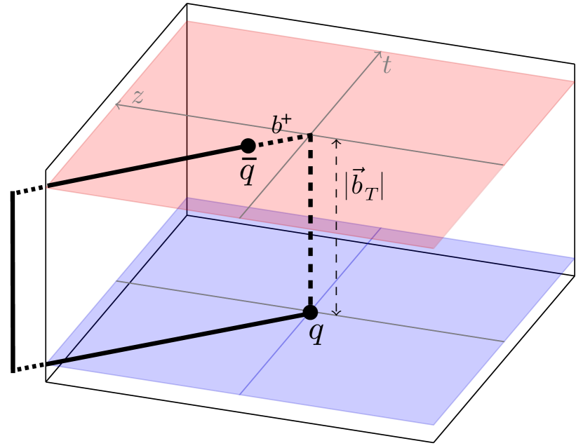
(a)

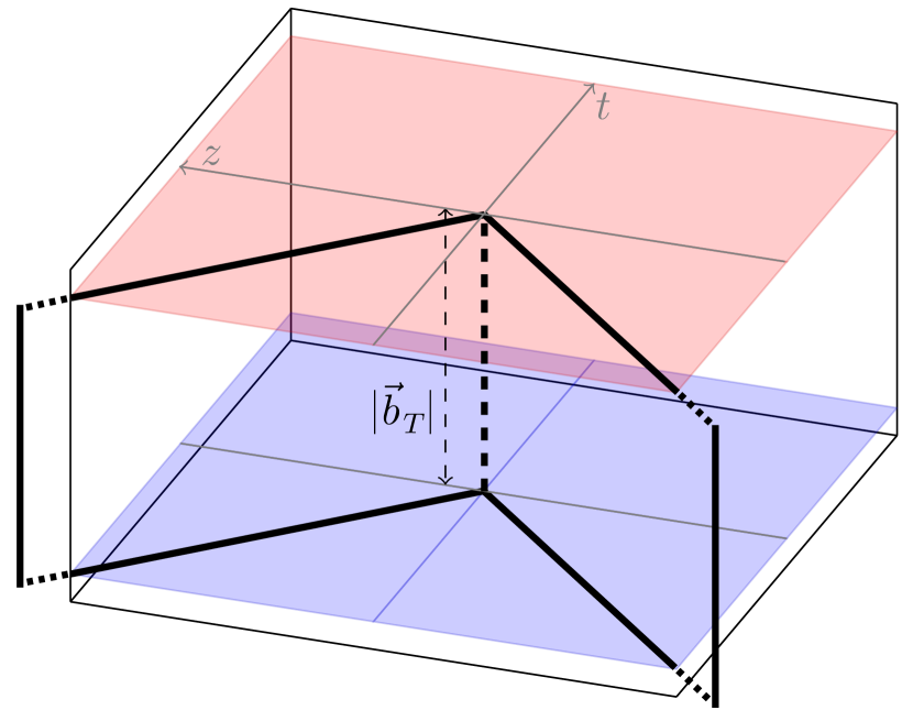
(b)

Figure 1: Illustration of the Wilson line structure of the $n$-collinear beam function $B_{q}$ (a) and the soft function $S^{q}$ (b), as given in eqs. (6) and (2.1). The solid Wilson lines extend to infinity in the directions indicated. Adapted from ref. Li:2016axz .

2.2 Definition of quasi-TMDPDFs

The quasi-TMDPDF is defined analogous to eq. (5), but as an equal-time correlator rather than a lightcone correlation function, namely

$$\tilde{f}_{q}(x,\vec{b}_{T},\mu,P^{z})=\lim_{\begin{subarray}{c}a\to 0\\ L\to\infty\end{subarray}}\int\!\frac{\mathrm{d}b^{z}}{2\pi}e^{\mathrm{i}b^{z}(xP^{z})} \tilde{Z}^{\prime}_{q}(b^{z},\mu,\tilde{\mu})\tilde{Z}_{\rm uv}^{q}(b^{z},\tilde{\mu},a)$$

$$\times\tilde{B}_{q}(b^{z},\vec{b}_{T},a,P^{z},L)\tilde{\Delta}_{S}^{q}(b_{T},a,L)\,.$$ (11)

Here $\tilde{B}_{q}$ is the quasi-beam function, $\tilde{\Delta}_{S}^{q}$ includes the quasi-soft function together with subtractions, $\tilde{Z}_{\rm uv}^{q}$ carries out UV renormalization in a lattice-friendly scheme, where $\tilde{\mu}$ stands for any added scales introduced by this scheme choice, and $\tilde{Z}_{q}^{\prime}$ converts the result perturbatively to the ${\overline{\mathrm{MS}}}$ scheme with scale $\mu$. Note that here, $L$ refers to the length of the Wilson lines in the definition of $\tilde{B}_{q}$ and $\tilde{\Delta}_{S}^{q}$ (see below), not the size of the lattice. The quasi beam and soft functions will be constructed such that all Wilson line self energies proportional to $L/a$ and $b_{T}/a$, as well as divergences $\propto L/b_{T}$ which correspond to rapidity divergences in the lightlike case Ji:2018hvs ; Ebert:2019okf , cancel between $\tilde{B}_{q}$ and $\tilde{\Delta}_{S}^{q}$. Therefore, the remaining UV renormalization $\tilde{Z}_{\rm uv}^{q}$ and the scheme conversion $\tilde{Z}^{\prime}_{q}$ only depend on $b^{z}$, but not necessarily $b_{T}$ or $L$. We keep implicit that finite lattice volume effects must be either removed or included as a systematic uncertainty.

The bare quasi-beam function is defined as

$$\tilde{B}_{q}(b^{z},\vec{b}_{T},a,P^{z},L)=\Bigl{<}\!h(P)\Big{|} \bar{q}(b^{\mu})W_{\hat{z}}(b^{\mu};L-b^{z})\frac{\Gamma}{2}W_{T}(L\hat{z};\vec{b}_{T},\vec{0}_{T})W^{\dagger}_{\hat{z}}(0;L)q(0)\Big{|}h(P)\!\Bigr{>}\,,$$ (12)

where $b^{\mu}=(0,\vec{b}_{T},b^{z})$, and the UV regulator is denoted as $a$, following the notation for the finite lattice spacing that acts as a UV regulator in lattice calculations. Due to the finite lattice size, the longitudinal Wilson lines are truncated at a length $L$ less than the size of the lattice, which also regulates the analog of rapidity divergences Ji:2018hvs ; Ebert:2019okf . Compared to eq. (6), we also replaced $\gamma^{-}$ by the Dirac structure $\Gamma$, which can be chosen as $\Gamma=\gamma^{0}$ or $\Gamma=\gamma^{z}$. (Technically, one can also use a combination, for example $\gamma^{0}+\gamma^{z}$.) The Wilson lines of finite length $L$ are defined by

$$W_{\hat{z}}(x^{\mu};L) =P\exp\left[-\mathrm{i}g\int_{L}^{0}\mathrm{d}s\,\mathcal{A}^{z}(x^{\mu}+s\hat{z})\right]\,,$$ (13)

while the transverse gauge links are identical to those in eq. (2.1).

For the quasi soft function, we use the bent soft function of ref. Ebert:2019okf , defined as

$$\tilde{S}^{q}_{\rm bent}(b_{T},a,L) =\frac{1}{N_{c}}\bigl{<}0\big{|}\mathrm{Tr}\bigl{\{}S^{\dagger}_{\hat{z}}(\vec{b}_{T};L)S_{-{\bar{n}}_{\perp}}\!(\vec{b}_{T};L)S_{T}(L{\bar{n}}_{\perp};\vec{b}_{T},\vec{0}_{T})$$

$$\hskip 56.9055pt\times S^{\dagger}_{-{\bar{n}}_{\perp}}\!(\vec{0}_{T};L)S_{\hat{z}}(\vec{0}_{T};L)S_{T}^{\dagger}\bigl{(}-L\hat{z};\vec{b}_{T},\vec{0}_{T}\bigr{)}\bigr{\}}\bigl{|}0\bigr{>}\,.$$ (14)

Here, ${\bar{n}}_{\perp}^{\mu}$ is the transverse unit vector orthogonal to $n_{\perp}^{\mu}=b_{\perp}^{\mu}/b_{T}$ and $\hat{z}$. Explicitly, if we parameterize $b_{T}^{\mu}=b_{T}(0,\cos\phi,\sin\phi,0)$, then $n_{\perp}^{\mu}=(0,\cos\phi,\sin\phi,0)$, and a valid choice for ${\bar{n}}_{\perp}^{\mu}$ is ${\bar{n}}_{\perp}^{\mu}=(0,-\sin\phi,\cos\phi,0)$. The Wilson lines in eq. (2.2) are defined as

$$S_{\hat{z}}(x^{\mu};L) =P\exp\biggl{[}-\mathrm{i}g\int_{-L}^{0}\mathrm{d}s\,\mathcal{A}^{z}(x^{\mu}+s\hat{z}^{\mu})\biggr{]}\,,$$

$$S_{-{\bar{n}}_{\perp}}\!(x^{\mu};L) =P\exp\biggl{[}-\mathrm{i}g\int_{-L}^{0}\mathrm{d}s\,{\bar{n}}_{\perp}\cdot\mathcal{A}(x^{\mu}-s{\bar{n}}_{\perp}^{\mu})\biggr{]}\,,$$

$$S_{T}(x^{\mu};\vec{b}_{T},\vec{0}_{T}) =P\exp\biggl{[}-\mathrm{i}g\int_{\vec{0}_{T}}^{\vec{b}_{T}}\mathrm{d}\vec{s}_{T}\cdot\vec{\mathcal{A}}_{T}(x^{\mu}+s_{T}^{\mu})\biggr{]}\,.$$ (15)

The Wilson line paths of both quasi beam and quasi soft function are illustrated in Fig. 2 for the choice $\phi=0$.

The quasi-soft factor is obtained from the bent soft function as

$$\tilde{\Delta}_{S}^{q}(b_{T},a,L)=\frac{\sqrt{\tilde{S}^{q}_{\rm bent}(b_{T},a,L)}}{\tilde{S}_{0}^{q}(b_{T},a,L)}=\frac{1}{\sqrt{\tilde{S}^{q}_{\rm bent}(b_{T},a,L)}}\,,$$ (16)

where $\tilde{S}_{0}^{q}=\tilde{S}^{q}_{\rm bent}$ is the subtraction factor which avoids double counting between quasi beam and soft functions. The overall length of the Wilson lines appearing in $\tilde{\Delta}_{S}^{q}$ must be chosen to ensure the cancellation of Wilson line self energies in eq. (2.2) Ebert:2019okf , whereas implementing this with the specific choice $\tilde{S}_{0}^{q}=\tilde{S}^{q}_{\rm bent}$ corresponds to a particular scheme.

Note that for the construction of the quasi-TMDPDF, different definitions of the quasi soft function could be employed as well. This yields different definitions of the quasi-TMDPDF, which will affect the (possibly nonperturbative) kernel relating quasi-TMDPDFs and TMDPDFs, see ref. Ebert:2019okf for a more detailed discussion. With the bent soft function in eq. (2.1), this relation was shown to be short distance dominated and hence perturbative at one loop, which motivates its use here. Importantly, for the determination of the Collins-Soper kernel the soft factor always cancels, such that this precise definition does not matter.

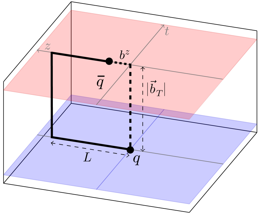
(a)

(b)

Figure 2: Illustration of the Wilson line structure of the quasi beam function $\tilde{B}_{q}$ (a) and the bent quasi soft function $\tilde{S}^{q}_{\rm bent}$ (b), as given in eqs. (12) and (2.2). Note the different coordinate systems in the two figures: (a) is shown in $(z,t,x)$ space, while (b) is shown in $(z,y,x)$ space. In both cases, $\vec{b}_{T}$ is aligned along the $x$ axis.

The spacelike Wilson lines of $\tilde{B}_{q}$ as given in eq. (12) and those of $\tilde{S}_{q}$ as given in eq. (2.2) give rise to self energies that yield power law divergences proportional to $e^{\delta m\,L_{\rm tot}}$. Here, $\delta m$ is a mass correction that absorbs divergences as $a\to 0$, and the total lengths of the Wilson line structures are given by $L_{\rm tot}^{B}=L+|L-b^{z}|+b_{T}$ for $\tilde{B}_{q}$ and $L_{\rm tot}^{S}=4L+2b_{T}$ for $\tilde{S}_{q}$, respectively. After combining the quasi beam function with the square root of the quasi soft function, the Wilson line self-energies yield the overall power-law divergence

$$e^{\delta m\,\bigl{(}L_{\rm tot}^{\rm B}-\frac{1}{2}L_{\rm tot}^{\rm S}\bigr{)}}=e^{-\delta m\,b^{z}}\,,\qquad(b^{z}<L)\,,$$ (17)

which has to be absorbed by $\tilde{Z}^{q}_{\rm uv}(b^{z},\tilde{\mu},a)$. To cancel this divergence on the lattice, the nonperturbative UV renormalization has to be applied before the Fourier transform, as shown in eq. (2.2), while in the lightlike case it is independent of $b^{z}$ and can be pulled out, see eq. (5). This distinction is important, implying in the ratio of TMDPDFs the UV renormalization factor $Z_{\rm uv}^{q}$ cancel out, whereas this is not possible for ratios of quasi-TMDPDFs.

2.3 Determination of the Collins-Soper kernel in momentum space

In this section, we briefly review the method proposed in ref. Ebert:2018gzl for calculating the Collins-Soper kernel from lattice QCD. As discussed in ref. Ebert:2018gzl , and in more detail in ref. Ebert:2019okf , in general there is a mismatch between the infrared structure of the quasi-beam function and beam function due to the fact that the latter requires a dedicated rapidity regulator, whereas the former has rapidity divergences regulated by the finite length $L$. This spoils the simplest boost picture from LaMET (even when supplemented by short distance corrections), for relating these proton matrix elements. Nevertheless, when combined with the quasi-soft and soft functions, these divergences and the $L$ dependence cancel, enabling the possibility of a matching equation between the quasi-TMDPDF and TMDPDF. However, even after these cancellations there can still be a mismatch in the remaining infrared structure of the quasi-soft and soft functions, leaving a relation of the form

$$\tilde{f}_{{\rm ns}}(x,\vec{b}_{T},\mu,P^{z}) =C_{{\rm ns}}\bigl{(}\mu,xP^{z}\bigr{)}g^{S}_{q}(b_{T},\mu)\exp\biggl{[}\frac{1}{2}\gamma_{\zeta}^{q}(\mu,b_{T})\ln\frac{(2xP^{z})^{2}}{\zeta}\biggr{]}f_{{\rm ns}}(x,\vec{b}_{T},\mu,\zeta)$$

$$\quad+\mathcal{O}\biggl{(}\frac{b_{T}}{L},\frac{1}{b_{T}P^{z}},\frac{1}{P^{z}L}\biggr{)}\,.$$ (18)

Here, $C_{{\rm ns}}$ is a perturbative kernel for the nonsinglet ${\rm ns}{=}u{-}d$ channel, $g_{q}^{S}$ is a nonperturbative contribution which reflects the mismatch in soft physics, and $\gamma_{\zeta}^{q}$ is the standard Collins-Soper kernel, which allows one to relate the TMDPDF at the scale $\zeta$ to the quasi-TMDPDF at proton momentum $P^{z}$. We assume the hierarchy of scales that $1/P^{z}\ll b_{T}\ll L$, such that corrections to this matching relation are suppressed for large $L$ and $P^{z}$, as indicated, and will be suppressed in the following. In ref. Ebert:2019okf it was shown that the bent soft function yields $g^{S}_{q}(b_{T},\mu)=1+{\cal O}(\alpha_{s}^{2})$. To demonstrate that eq. (2.3) is a true matching equation requires an all-order proof that $g^{S}_{q}(b_{T},\mu)=1$, which has not been demonstrated. However the lack of this proof does not impact the determination of the anomalous dimension $\gamma_{\zeta}^{q}(\mu,b_{T})$, to which we now turn.

Evaluating eq. (2.3) at two different proton momenta $P^{z}_{1}\neq P^{z}_{2}$ but the same $\zeta$, and taking the ratio of the results yields

$$\frac{\tilde{f}_{{\rm ns}}(x,\vec{b}_{T},\mu,P^{z}_{1})}{\tilde{f}_{{\rm ns}}(x,\vec{b}_{T},\mu,P^{z}_{2})}=\frac{C_{{\rm ns}}\bigl{(}\mu,xP^{z}_{1}\bigr{)}}{C_{{\rm ns}}\bigl{(}\mu,xP^{z}_{2}\bigr{)}}\exp\biggl{[}\gamma_{\zeta}^{q}(\mu,b_{T})\ln\frac{P^{z}_{1}}{P^{z}_{2}}\biggr{]}\,.$$ (19)

Here $g_{q}^{S}$ and $f_{{\rm ns}}$ have dropped out. In ref. Ebert:2018gzl , this was solved for $\gamma_{\zeta}^{q}$ as

$$\gamma^{q}_{\zeta}(\mu,b_{T}) =\frac{1}{\ln(P^{z}_{1}/P^{z}_{2})}\ln\frac{C_{\rm ns}(\mu,xP_{2}^{z})\,\tilde{f}_{\rm ns}(x,\vec{b}_{T},\mu,P^{z}_{1})}{C_{\rm ns}(\mu,xP_{1}^{z})\,\tilde{f}_{\rm ns}(x,\vec{b}_{T},\mu,P^{z}_{2})}\,.$$ (20)

On the lattice one obtains the quasi-TMDPDF by Fourier transforming a position-space correlation function to momentum space, as given in eq. (2.2). Inserting eq. (2.2) into eq. (20), one then obtains Ebert:2018gzl

$$\gamma^{q}_{\zeta}(\mu,b_{T}) =\frac{1}{\ln(P^{z}_{1}/P^{z}_{2})}$$ (21)

$$\times\ln\frac{C_{\rm ns}(\mu,xP_{2}^{z})\,\int\!\mathrm{d}b^{z}\,e^{ib^{z}xP_{1}^{z}}\,\tilde{Z}_{q}^{\prime}(b^{z},\mu,\tilde{\mu})\,\tilde{Z}_{\rm uv}^{q}(b^{z},\tilde{\mu},a)\,\tilde{B}_{\rm ns}(b^{z},\vec{b}_{T},a,P_{1}^{z},L)}{C_{\rm ns}(\mu,xP_{1}^{z})\,\int\!\mathrm{d}b^{z}\,e^{ib^{z}xP_{2}^{z}}\,\tilde{Z}_{q}^{\prime}(b^{z},\mu,\tilde{\mu})\,\tilde{Z}_{\rm uv}^{q}(b^{z},\tilde{\mu},a)\,\tilde{B}_{\rm ns}(b^{z},\vec{b}_{T},a,P_{2}^{z},L)}\,.$$

Note that here we have canceled the quasi soft factor $\tilde{\Delta}_{S}^{q}(b_{T},a,L)$ in the ratio, as it is independent of $b^{z}$. The advantage of doing so is that one needs to calculate one less nonperturbative function from lattice QCD. The price to pay is that $\tilde{B}_{\rm ns}$ still contains Wilson line self energies $\propto L/a,b_{T}/a$ and divergences $\propto L/b_{T}$, which now only cancel in the ratio rather than in the numerator and denominator, respectively. To achieve the separate cancellation, we can simultaneously insert a $b^{z}$-independent factor ${\tilde{R}}_{B}$ in both the numerator and denominator to separately cancel these leftover divergences,

$$\gamma^{q}_{\zeta}(\mu,b_{T})=\frac{1}{\ln(P^{z}_{1}/P^{z}_{2})}$$ (22)

$$\times\ln\frac{C_{\rm ns}(\mu,xP_{2}^{z})\,\int\!\mathrm{d}b^{z}\,e^{ib^{z}xP_{1}^{z}}\,\tilde{Z}_{q}^{\prime}(b^{z},\mu,\tilde{\mu})\,\tilde{Z}_{\rm uv}^{q}(b^{z},\tilde{\mu},a)\,{\tilde{R}}_{B}(b_{T},\tilde{\mu},a,L)\,\tilde{B}_{\rm ns}(b^{z},\vec{b}_{T},a,P_{1}^{z},L)}{C_{\rm ns}(\mu,xP_{1}^{z})\,\int\!\mathrm{d}b^{z}\,e^{ib^{z}xP_{2}^{z}}\,\tilde{Z}_{q}^{\prime}(b^{z},\mu,\tilde{\mu})\,\tilde{Z}_{\rm uv}^{q}(b^{z},\tilde{\mu},a)\,{\tilde{R}}_{B}(b_{T},\tilde{\mu},a,L)\,\tilde{B}_{\rm ns}(b^{z},\vec{b}_{T},a,P_{2}^{z},L)}\,.$$

This factor has to be constructed such that it exactly removes all divergences that would normally be canceled by $\tilde{\Delta}_{S}^{q}(b_{T},a,L)$, i.e. all power-law divergences not yet absorbed by $\tilde{Z}_{\rm uv}^{q}(b^{z},\tilde{\mu},a)$. One trivial choice for this factor is thus to use the soft factor that was canceled before, ${\tilde{R}}_{B}=\tilde{\Delta}_{S}^{q}$, while another simple choice would be ${\tilde{R}}_{B}=[\tilde{B}_{\rm ns}(0,\vec{b}_{T},a,P_{R}^{z},L)]^{-1}$, i.e. the quasi beam function at vanishing separation $b^{z}=0$ and some reference momentum $P_{R}^{z}$. In Sec. 3, we will construct a more refined expression by using the nonperturbative RI^′/MOM renormalization factor in a similar fashion, and the final definition for the combination $\tilde{Z}_{\rm uv}^{q}{\tilde{R}}_{B}$ will be given in eq. (3).

As stressed in ref. Ebert:2018gzl , eqs. (21) and (22) are formally independent of $x$, $P_{1}^{z}$ and $P_{2}^{z}$, up to power corrections as indicated in eq. (2.3), such that one can use any residual dependence of the lattice results on these parameters to assess systematic uncertainties.

The one-loop result for the matching coefficient $C_{\rm ns}$ that enters eq. (21), when $\tilde{f}_{\rm ns}$, $\tilde{Z}_{q}^{\prime}$ and $\gamma_{\zeta}^{q}$ are in the ${\overline{\mathrm{MS}}}$ scheme, has been calculated in refs. Ebert:2018gzl ; Ebert:2019okf and is given by

$$C_{{\rm ns}}\bigl{(}\mu,xP^{z}\bigr{)} =1+\frac{\alpha_{s}C_{F}}{4\pi}\biggl{[}-\ln^{2}\frac{(2xP^{z})^{2}}{\mu^{2}}+2\ln\frac{(2xP^{z})^{2}}{\mu^{2}}-4+\frac{\pi^{2}}{6}\biggr{]}+\mathcal{O}(\alpha_{s}^{2})\,.$$ (23)

This short distance coefficient can also be extracted from the results of ref. Ji:2018hvs . Note that $C_{{\rm ns}}$ is an even function of its second argument, $C_{{\rm ns}}(\mu,-xP^{z})=C_{{\rm ns}}(\mu,xP^{z})$.

2.4 Determination of the Collins-Soper kernel in position space

A potential drawback of using eq. (21) and eq. (22) is that one has to Fourier transform the position-space correlator $\tilde{B}_{{\rm ns}}(b^{z},\vec{b}_{T},a,P^{z},L)$. This can be a limiting factor, as only a finite number of $b^{z}$ values are available from lattice, which thus does not fully determine the quasi beam function (often referred to as an inverse problem). We hence propose in this section a related but modified formula which enables the matching to be performed directly in position space, thus providing an alternate method to carry out the calculation and test systematic uncertainties.

To derive this relation, we need the Fourier transforms of the quasi TMDPDF,

$$\tilde{f}_{\rm ns}(x,\vec{b}_{T},\mu,P^{z}) =\int\frac{\mathrm{d}b^{z}}{2\pi}e^{\mathrm{i}(xP^{z})b^{z}}\tilde{f}_{\rm ns}(b^{z},\vec{b}_{T},\mu,P^{z})\,.$$ (24)

Here, $\tilde{f}_{\rm ns}(x,\vec{b}_{T},\mu,P^{z})$ is the quasi-TMDPDF defined previously in momentum space, which is now expressed in terms of its Fourier-transform $\tilde{f}_{\rm ns}(b^{z},\vec{b}_{T},\mu,P^{z})$ in position space on the right hand side of eq. (24). The advantage of working with the latter is its direct connection to the quasi-beam function $\tilde{B}(b^{z},\vec{b}_{T},a,P^{z},L)$, which is the object actually calculated on the lattice. Note that for simplicity we distinguish the quasi-TMDPDF in position and momentum space only by their arguments, as it is always clear from context which one we refer to. It will be convenient to work with the Fourier transform of the inverse of the kernel $C_{\rm ns}$, defined through

$$\bar{C}_{\rm ns}(\mu,b^{z}P^{z},P^{z}) \equiv\int\!\mathrm{d}x\,e^{-\mathrm{i}x(b^{z}P^{z})}\,\bigl{[}C_{\rm ns}(\mu,xP^{z})\bigr{]}^{-1}\,,$$

$$\bigl{[}C_{\rm ns}(\mu,xP^{z})\bigr{]}^{-1} =\int\frac{\mathrm{d}(b^{z}P^{z})}{2\pi}\,e^{\mathrm{i}x(b^{z}P^{z})}\,\bar{C}_{\rm ns}(\mu,b^{z}P^{z},P^{z})\,.$$ (25)

Plugging eqs. (24) and (2.4) back into eq. (19), we get

$$P^{z}_{1}\int\mathrm{d}b^{z}_{1}\,\mathrm{d}{b^{z}_{1}}^{\prime}\,e^{\mathrm{i}xP^{z}_{1}(b^{z}_{1}+{b^{z}_{1}}^{\prime})}\bar{C}_{\rm ns}(\mu,{b^{z}_{1}}^{\prime}P^{z}_{1},P^{z}_{1})\tilde{f}_{\rm ns}(b^{z}_{1},\vec{b}_{T},\mu,P^{z}_{1})$$ (26)

$$=~{} P^{z}_{2}\int\mathrm{d}b^{z}_{2}\,\mathrm{d}{b^{z}_{2}}^{\prime}\,e^{\mathrm{i}xP^{z}_{2}(b^{z}_{2}+{b^{z}_{2}}^{\prime})}\bar{C}_{\rm ns}(\mu,{b^{z}_{2}}^{\prime}P^{z}_{2},P^{z}_{2})\tilde{f}_{\rm ns}(b^{z}_{2},\vec{b}_{T},\mu,P^{z}_{2})\ \exp\biggl{[}\gamma_{\zeta}^{q}(\mu,b_{T})\ln\frac{P^{z}_{1}}{P^{z}_{2}}\biggr{]}\,.$$

Next, we Fourier transform both sides from momentum fraction $x$ to a dimensionless position $y$, by multiplying by $e^{-\mathrm{i}xy}$ and integrating over $x$, obtaining

$$\int\mathrm{d}b^{z}_{1}\,\bar{C}_{\rm ns}(\mu,y-b^{z}_{1}P^{z}_{1},P^{z}_{1})\tilde{f}_{\rm ns}(b^{z}_{1},\vec{b}_{T},\mu,P^{z}_{1})$$ (27)

$$=~{} \int\mathrm{d}b^{z}_{2}\,\bar{C}_{\rm ns}(\mu,y-b^{z}_{2}P^{z}_{2},P^{z}_{2})\tilde{f}_{\rm ns}(b^{z}_{2},\vec{b}_{T},\mu,P^{z}_{2})\ \exp\biggl{[}\gamma_{\zeta}^{q}(\mu,b_{T})\ln\frac{P^{z}_{1}}{P^{z}_{2}}\biggr{]}\,.$$

This can trivially be solved for $\gamma_{\zeta}^{q}$ as

$$\gamma_{\zeta}^{q}(\mu,b_{T})=\frac{1}{\ln(P^{z}_{1}/P^{z}_{2})}\ln\frac{\int\!\mathrm{d}b^{z}\,\bar{C}_{\rm ns}(\mu,y-b^{z}P^{z}_{1},P^{z}_{1})\tilde{f}_{\rm ns}(b^{z},\vec{b}_{T},\mu,P^{z}_{1})}{\int\!\mathrm{d}b^{z}\,\bar{C}_{\rm ns}(\mu,y-b^{z}P^{z}_{2},P^{z}_{2})\tilde{f}_{\rm ns}(b^{z},\vec{b}_{T},\mu,P^{z}_{2})}\,.$$ (28)

As expected, Fourier transforming the product in eq. (19) yields a convolution in position space. In eq. (28), $\tilde{f}_{\rm ns}$ is the renormalized nonsinglet quasi-TMDPDF in position-space as calculated on lattice.

Using the expression eq. (2.2) for $\tilde{f}_{\rm ns}$, we obtain the final expression

$$\gamma_{\zeta}^{q}(\mu,b_{T})=\frac{1}{\ln(P^{z}_{1}/P^{z}_{2})}$$ (29)

$$\times\ln\frac{\int\!\mathrm{d}b^{z}\,\bar{C}_{\rm ns}(\mu,y-b^{z}P^{z}_{1},P^{z}_{1})\,\tilde{Z}^{\prime}_{q}(b^{z},\mu,\tilde{\mu})\,\tilde{Z}_{\rm uv}^{q}(b^{z},\tilde{\mu},a)\,{\tilde{R}}_{B}(b_{T},\tilde{\mu},a,L)\,\tilde{B}_{\rm ns}(b^{z},\vec{b}_{T},a,P^{z}_{1},L)}{\int\!\mathrm{d}b^{z}\,\bar{C}_{\rm ns}(\mu,y-b^{z}P^{z}_{2},P^{z}_{2})\,\tilde{Z}^{\prime}_{q}(b^{z},\mu,\tilde{\mu})\,\tilde{Z}_{\rm uv}^{q}(b^{z},\tilde{\mu},a)\,{\tilde{R}}_{B}(b_{T},\tilde{\mu},a,L)\,\tilde{B}_{\rm ns}(b^{z},\vec{b}_{T},a,P^{z}_{2},L)}\,,$$

where we suppress the explicit limits $L\to\infty$ and $a\to 0$ for simplicity. As in eq. (22), we have inserted a factor ${\tilde{R}}_{B}$ that cancels all divergences in $L/a,b_{T}/a$ and $L/b_{T}$ separately in the numerator and denominator, which otherwise would only cancel in the ratio. Again, formally the dependence of the right hand side of eq. (29) on $y$, $P^{z}_{1}$ and $P^{z}_{2}$ cancels up to power corrections, such that one can use any residual dependence of the lattice results on these parameters to assess systematic uncertainties. To use the improved formula in eq. (29) one only needs the position-space proton matrix element $\tilde{B}_{\rm ns}$ (directly obtained on the lattice), its renormalization factor $\tilde{Z}_{\rm uv}^{q}$ (also obtained on the lattice) combined with the factor ${\tilde{R}}_{B}$ (discussed in Sec. 3), the ${\overline{\mathrm{MS}}}$-conversion factor $\tilde{Z}^{\prime}_{q}$ (which we calculate in Secs. 3 and 4 of this paper), and the Fourier-transformed matching kernel $\bar{C}_{\rm ns}$ (which we obtain below).

In both eqs. (22) and (29) the dominant contributions to the integrals come from the small $b^{z}$ region. In the convolution in eq. (29) the kernel $\bar{C}_{\rm ns}(y-b^{z}P^{z})$ given below is peaked around $b^{z}P^{z}\sim y$, while contributions from the region $|b^{z}P^{z}-y|\gg 1$ are suppressed by this kernel. In comparison, the Fourier transform in eq. (22) is dominated by $xP^{z}b^{z}\sim 1$ and becomes less sensitive to $b^{z}\gg 1/(xP^{z})$ due to suppression by the phase factor $\exp(ixP^{z}b^{z})$. In practice, we can implement both methods on the lattice and compare their systematic uncertainties.

Note that we have chosen the definition eq. (2.4) of the position-space kernel $\bar{C}_{\rm ns}$ to be determined by the transform of the inverse of $C_{\rm ns}$ in order to make eq. (29) particularly simple, with a numerator depending only on the momentum $P^{z}_{1}$ and the denominator only on $P^{z}_{2}$. For comparison and completeness, we present in appendix B the corresponding derivation when using a position-space kernel $\bar{C}_{\rm ns}^{\prime}$ that is defined by the transform of $C_{\rm ns}$ itself, in which case numerator and denominator would both depend on $P^{z}_{1}$ and $P^{z}_{2}$.

The Fourier transform $\bar{C}_{\rm ns}$ can be further simplified by employing that in the physical limit $L,P^{z}\to\infty$, $\tilde{f}_{q}$ has limited support $x\in[0,1]$ for quarks and $x\in[-1,0]$ for antiquarks. Hence, we can make different choices for the integration range in eq. (2.4) which lead to formally equivalent results when the resulting coefficients $\bar{C}_{\rm ns}$ are employed in eq. (29). To exploit this freedom we consider the two natural choices, defining

$$\bar{C}_{\rm ns}^{[0,1]}(\mu,b^{z}P^{z},P^{z}) =\int_{0}^{1}\!\mathrm{d}x\,e^{-\mathrm{i}x(b^{z}P^{z})}\,\bigl{[}C_{\rm ns}(\mu,xP^{z})\bigr{]}^{-1}\,,$$ (30)

$$\bar{C}_{\rm ns}^{[-1,1]}(\mu,b^{z}P^{z},P^{z}) =\int_{-1}^{1}\!\mathrm{d}x\,e^{-\mathrm{i}x(b^{z}P^{z})}\,\bigl{[}C_{\rm ns}(\mu,xP^{z})\bigr{]}^{-1}\,,$$ (31)

where the superscript in $\bar{C}_{\rm ns}^{D}$ denotes the integration domain $D$.

Physically, $\bar{C}_{\rm ns}^{[0,1]}$ as defined in eq. (30) corresponds to the kernel for a quark quasi-TMDPDF, while $\bar{C}_{\rm ns}^{[-1,0]}=\bigl{(}\bar{C}_{\rm ns}^{[0,1]}\bigr{)}^{*}$ would correspond to an antiquark. Eq. (31) thus corresponds to the sum of quark and antiquark contributions. Since in eq. (29) we only employ the nonsinglet channel ${\rm ns}{=}u{-}d$, the antiquark contribution must cancel, and one can equivalently employ the unrestricted $x$ integration in eq. (2.4), or one of the restricted versions in eq. (30) or eq. (31), for the kernel entering eq. (29). In practice, there will be a remnant contribution from antiquarks since one does not work in the physical limit $L,P^{z}\to\infty$. Hence one can employ the difference between eqs. (2.4), (30) and (31) as a further handle to probe systematic uncertainties from working at finite momentum. Note that since $C_{\rm ns}$ depends logarithmically on $xP^{z}/\mu$, its Fourier transform according to eq. (2.4) with unconstrained integration range will involve plus distributions which are complicated to implement numerically, so here we will refrain from advocating for using the unrestricted integration, and hence only present the simpler results obtained using eqs. (30) and (31).

Matching kernel in position space.

Next we explicitly calculate the Fourier transform of $C_{\rm ns}$ to position space as defined in eqs. (30) and (31). $C_{\rm ns}$ was calculated at next-to-leading order (NLO) in the ${\overline{\mathrm{MS}}}$ scheme in refs. Ebert:2018gzl ; Ebert:2019okf and is given in eq. (23). Perturbatively inverting it gives the one-loop result

$$\bigl{[}C_{{\rm ns}}\bigl{(}\mu,xP^{z}\bigr{)}\bigr{]}^{-1} =1+\frac{\alpha_{s}C_{F}}{4\pi}\biggl{[}\ln^{2}\frac{(2xP^{z})^{2}}{\mu^{2}}-2\ln\frac{(2xP^{z})^{2}}{\mu^{2}}+4-\frac{\pi^{2}}{6}\biggr{]}+\mathcal{O}(\alpha_{s}^{2})\,.$$ (32)

Fourier transform according to eqs. (30) and (31), we obtain

$$\bar{C}_{\rm ns}^{D}(\mu,y,P^{z}) =f_{0}^{D}(y)+\frac{\alpha_{s}C_{F}}{4\pi}\Bigl{[}f_{2}^{D}(y)+(2L_{z}-2)f_{1}^{D}(y)+\Bigl{(}L_{z}^{2}-2L_{z}+4-\frac{\pi^{2}}{6}\Bigr{)}f_{0}^{D}(y)\Bigl{]}$$

$$\quad+\mathcal{O}(\alpha_{s}^{2})\,,$$ (33)

where we abbreviated $L_{z}=\ln[(2P^{z}/\mu)^{2}]$, and as before the superscript $D$ on the three required functions $f_{i}^{D}(y)$ denotes the integration range of the Fourier transform.

For the case of integrating over $D=[0,1]$ the auxiliary integrals are

$$f_{n}^{[0,1]}(y) =\int_{0}^{1}\mathrm{d}x\,e^{-\mathrm{i}xy}\ln^{n}(x^{2})$$

$$=(-2)^{n}n!~{}{}_{n+1}F_{n+1}\bigl{(}\{1,\cdots,1\},\{2,\cdots,2\},-\mathrm{i}y\bigr{)}\,.$$ (34)

Here, ${}_{n}F_{n}$ is a hypergeometric function. The results for $n=0$ and $n=1$ can be expressed using standard functions,

$$f_{0}^{[0,1]}(y) =\frac{1-e^{-\mathrm{i}y}}{\mathrm{i}y}\,,\qquad f_{1}^{[0,1]}(y)=\frac{2\mathrm{i}}{y}\bigl{[}\Gamma(0,\mathrm{i}y)+\ln(\mathrm{i}y)+\gamma_{E}\bigr{]}\,.$$ (35)

On the other hand, for the case of integrating over $D=[-1,1]$ the auxiliary integrals are

$$f_{n}^{[-1,1]}(y) =\int_{-1}^{1}\mathrm{d}x\,e^{-\mathrm{i}xy}\ln^{n}(x^{2})=2\,{\rm Re}\bigl{[}f_{n}^{[0,1]}(y)\bigr{]}\,.$$ (36)

For $n=0$ and $n=1$, we obtain the simple results

$$f_{0}^{[-1,1]}(y) =2\frac{\sin y}{y}\,,\qquad f_{1}^{[-1,1]}(y)=-4\frac{\mathrm{Si}(y)}{y}\,,$$ (37)

where ${\rm Si}(y)=\int_{0}^{y}dt\,\sin(t)/t$ is the sine integral function.

Note that the above functions behave as $f_{n}^{D}(y)\sim 1/y$ for large $y$ and oscillate, and hence the dominant contribution to the convolutions in eqs. (28) and (29) is given by $y-b^{z}P^{z}\sim 1$. This naturally limits the impact of the quasi beam function from large $b^{z}$.

3 RI^′/MOM renormalization and matching

The determination of $\gamma_{\zeta}^{q}$ using either eq. (22) or (29) requires calculating the quasi-beam function $\tilde{B}_{q}$ from lattice, a renormalization of UV divergences with $\tilde{Z}_{\rm uv}^{q}$, a definition of ${\tilde{R}}_{B}$ to cancel remaining power-law divergences (one choice would be $\tilde{\Delta}_{S}^{q}$), and finally $\tilde{Z}_{q}^{\prime}$ to convert to the ${\overline{\mathrm{MS}}}$ scheme. Here, we specify in detail a preferred choice for how to construct these nonperturbative renormalization factors in the RI^′/MOM scheme, and how the conversion factor $\tilde{Z}_{q}^{\prime}$ can be calculated perturbatively. $\tilde{Z}_{q}^{\prime}$ is then calculated at one loop in Sec. 4.

Note that for $b^{z}{=}0$, the corresponding ${\overline{\mathrm{MS}}}$ conversion kernel for the quasi beam function $\tilde{B}_{q}$ has been calculated in ref. Constantinou:2019vyb , which is sufficient for the lattice studies of the $x$-moments of TMDPDFs carried out in refs. Musch:2010ka ; Musch:2011er ; Engelhardt:2015xja ; Yoon:2016dyh ; Yoon:2017qzo , but does not suffice for the determination of the Collins-Soper kernel which requires the calculation for nonvanishing $b^{z}$.

To renormalize the staple-shaped Wilson line operators entering the quasi beam function on the lattice, we need to prove their renormalizability first. Under lattice regularization, Lorentz symmetry group is broken into the hypercubic group, so it is more involved to employ standard field theory techniques to make this proof. Nevertheless, it has been proven that lattice gauge theory is renormalizable to all orders of perturbation theory within the functional formalism Reisz:1988kk , which also stands for the case with a background gauge field Luscher:1995vs . Therefore, the counterterms to the lattice action are only those allowed by gauge and hypercubic symmetries. This proof is also applicable to composite operators, which is the basis for their nonperturbative renormalization on the lattice. Therefore, we expect the renormalization of staple-shaped Wilson line operators to be similar in both continuum and lattice perturbation theories, except that in the latter there can be novel counterterms allowed by lattice symmetries. To begin with, we argue that in continuum theory the staple-shaped quark Wilson line operator can be renormalized multiplicatively in position space as

$$\mathcal{O}_{0}^{\Gamma}(b^{\mu},\Lambda,L) \equiv\bar{\psi}_{0}(b^{\mu})W_{\hat{z}}\frac{\Gamma}{2}W_{T}W^{\dagger}_{\hat{z}}\psi_{0}(0)$$

$$=Z_{q,\rm wf}\,e^{\delta m(L+|L-b^{z}|+b_{T})}\Bigl{(}\bar{\psi}(b^{\mu})W_{\hat{z}}\frac{\Gamma}{2}W_{T}W^{\dagger}_{\hat{z}}\psi(0)\Bigr{)}_{R}$$

$$\equiv\tilde{Z}_{B}\Bigl{(}\bar{\psi}(b^{\mu})W_{\hat{z}}\frac{\Gamma}{2}W_{T}W^{\dagger}_{\hat{z}}\psi(0)\Bigr{)}_{R}\,,$$ (38)

where $\Lambda$ is a generic UV regulator that respects Lorentz invariance and gauge invariance. Here, $W_{\hat{z}}$ and $W_{T}$ are Wilson lines as defined in eqs. (2.1) and (13), and for brevity we suppressed their explicit arguments, which are given in eq. (12). In the first line in eq. (3), we work with bare quark fields $\psi_{0}$ and Wilson lines built of bare gluon fields and bare couplings, while in the second line we work with renormalized fields and couplings, indicated by the subscript $R$. $Z_{q,\rm wf}$ includes all the logarithmic UV divergences originating from the wave function renormalization and the quark-Wilson-line vertices. The exponential absorbs all linear power divergences from the self-energies of the spacelike Wilson lines, where $L+|L-b^{z}|+b_{T}$ is the total length of the staple.

Eq. (3) resembles the multiplicative renormalization for the straight Wilson line operators, for which the renormalization in the RI^′/MOM scheme has been studied in ref. Constantinou:2017sej ; Stewart:2017tvs ; Chen:2017mzz ; Alexandrou:2017huk ; Liu:2018uuj . For the staple-shaped operators discussed here, the multiplicative renormalization has also been used in ref. Constantinou:2019vyb , which carried out the RI^′/MOM renormalization for the special case $b^{z}=0$, i.e. vanishing longitudinal separation of the staple. The proof of eq. (3) is analogous to that for the straight Wilson line operators, where one employs the auxiliary field formalism Dorn:1986dt ; Ji:2017oey ; Green:2017xeu ; Zhang:2018diq . This auxiliary field formalism is also commonly used to derive Wilson line operators in the Soft Collinear Effective Theory, see the original work in Refs. Bauer:2001yt ; Bauer:2002nz . For the TMD, by using three independent auxiliary “heavy quark” fields for each edge of the staple-shaped Wilson line, the nonlocal quark Wilson line operator can be reduced to the product of four composite operators in the effective theory that includes these auxiliary fields. BRST invariance implies that this effective theory is renormalizable through multiplicative counterterms to all orders in perturbation theory Ji:2017oey . It follows that in continuum QCD, the staple-shaped quark Wilson line operator can indeed be renormalized multiplicatively as shown in eq. (3).

On the discretized lattice where $\Lambda\to 1/a$, we can also use the auxiliary field theory to replicate the proof, and hypercubic symmetry does not allow the operator to have UV-divergent mixings with other operators with the same or lower dimensions. Though mixing with higher-dimensional operators is allowed, it is power suppressed and not relevant when one takes the continuum limit $a\to 0$. However, as pointed out in refs. Constantinou:2019vyb ; Yoon:2017qzo , due to the breaking of chiral symmetries, there will be mixing with other operators on a discretized lattice, and thus the renormalization on lattice requires an independent study Yoon:2017qzo ; Shanahan:2019zcq . After lattice renormalization of the quasi beam function, its continuum limit can be taken and the result is independent of the UV regulator, which allows us to calculate the scheme conversion factors in continuum perturbation theory with dimensional regularization. In this work, we will discuss how to renormalize the quasi beam function in the RI^′/MOM scheme on the lattice, and then focus on its conversion to the ${\overline{\mathrm{MS}}}$ scheme in continuum perturbation theory. Since one-loop lattice perturbation theory Constantinou:2019vyb suggests that the mixing due to chiral-symmetry breaking is zero for certain choices of $\Gamma$, while for the other choices the mixings can be reduced by tuning the parameters of lattice action, we do not consider this effect in our calculation by assuming that either a proper choice of $\Gamma$ is made or the mixings are sufficiently small with fine-tuned lattice parameters.

To implement the RI^′/MOM scheme for the quasi beam function, one first computes the amputated Green’s function of the operator given in eq. (3),

$$\Lambda^{\Gamma}_{0}(b,a,p,L)\equiv\left[S^{-1}_{0}(p,a)\right]^{\dagger}\sum_{x,y}e^{ip\cdot(x-y)}\big{\langle}0\big{|}T\bigl{[}\psi_{0}(x,a){\cal O}_{0}^{\Gamma}(b^{\mu},a,L)\bar{\psi}_{0}(y,a)\bigr{]}\big{|}0\big{\rangle}S^{-1}_{0}(p,a)\,,$$ (39)

which is also referred to as the vertex function. Here and below $b$ indicates dependence on $b^{z}$ and $b_{T}$. In eq. (39), $S_{0}(p,a)$ is the bare quark propagator that can be calculated nonperturbatively on the lattice. $\Lambda^{\Gamma}_{0}(b,a,p,L)$ is a linear combination of Dirac matrices that are allowed by the symmetries of space-time and the operator itself. For off-shell quarks, there will also be finite mixing with equation-of-motion operators that vanish in the on-shell limit. Furthermore, the off-shell matrix element is not gauge invariant, and thus one has to fix a particular gauge choice as part of the renormalization scheme, which in lattice QCD is typically chosen as the Landau gauge.

In practice, one needs to choose a projection operator $\mathcal{P}$ to define the off-shell matrix element of the quasi-beam function from the amputated Green’s function,

$$\tilde{q}^{\Gamma\cal,P}_{0}(b,a,p,L)={\rm tr}\bigl{[}\Lambda^{\Gamma}_{0}(b,a,p,L)\mathcal{P}\bigr{]}\,.$$ (40)

The choice of $\mathcal{P}$ is not unique Stewart:2017tvs ; Liu:2018uuj , but it must have overlap with $\Gamma$ to project out all the UV divergences as $a\to 0$. In ref. Constantinou:2017sej ; Constantinou:2019vyb , the choice is ${\mathcal{P}}=\Gamma$, while in refs. Stewart:2017tvs ; Liu:2018uuj both the choice ${\mathcal{P}}=\not{p}$, and a choice for $\mathcal{P}$ that effectively projects out the coefficient of $\Gamma$ in the covariant decomposition of $\Lambda^{\Gamma}_{0}$, were considered. In principle, the dependence on the projection $\mathcal{P}$ will be canceled by the scheme conversion factor, since the ${\overline{\mathrm{MS}}}$ renormalization constant is unique. But in practice, since the conversion factor is computed at fixed orders in perturbation theory, there can still be remnant $\mathcal{P}$ dependence at higher orders, which is part of the systematic uncertainty.

In the RI^′/MOM scheme, the renormalization constant $\tilde{Z}_{B}^{\Gamma,\mathcal{P}}$ of the bare operator $\mathcal{O}_{0}^{\Gamma}$ defined in eq. (3) is determined by requiring that at a specific momentum $p_{R}^{\mu}$, the projection defined in eq. (40) reduces to its value at tree level in perturbation theory. Here, we actually need to define the RI^′/MOM condition for the quasi-TMDPDF, which also includes the soft factor. It reads

$$\tilde{Z}^{\Gamma,\mathcal{P}}_{q}(b^{z},b_{T}^{R},p_{R},a)\,Z_{\rm wf}(p_{R},a)\,\lim_{L\to\infty}\tilde{q}^{\Gamma,\mathcal{P}}_{0}(b,a,p,L)\,\tilde{\Delta}_{S}^{q}(b_{T},a,L)\bigg{|}_{\stackrel{{\scriptstyle p^{\mu}=p_{R}^{\mu}}}{{b_{T}=b_{T}^{R}}}}$$

$$=\tilde{q}^{\Gamma,\mathcal{P}}_{\rm tree}(b^{z},b_{T}^{R},p_{R})\,.$$ (41)

Here, $q^{\Gamma,\mathcal{P}}_{\rm tree}$ is the value of eq. (40) at tree-level in perturbation theory, which is nonzero only for particular choices of $\Gamma$ and $\mathcal{P}$, and each such pair $(\Gamma,\mathcal{P})$ define a particular $\tilde{Z}_{q}^{\Gamma,\mathcal{P}}$. The tree level soft factor is given by $\tilde{\Delta}_{S\,\rm tree}^{q}=1$ and hence not explicitly given in eq. (3). Here the choice for the scales $p_{R}$ and $b_{T}^{R}$ are part of the definition of the RI^′/MOM scheme.

In eq. (3), the wave function renormalization factor $Z_{\rm wf}$ arises to compensate for the renormalization of the bare quark fields in eq. (39). It is determined independently with the following condition on the quark propagator,

$$\bigl{[}Z_{\rm wf}(p,a)\bigr{]}^{-1}S_{0}(p,a)\big{|}_{p^{2}=p_{R}^{2}}=S_{\rm tree}(p_{R},a)$$

$$\Rightarrow~{} \bigl{[}Z_{\rm wf}(p_{R},a)\bigr{]}^{-1}=\frac{1}{4}{\rm tr}\bigl{[}S^{-1}_{0}(p,a)S_{\rm tree}(p,a)\bigr{]}_{p^{2}=p_{R}^{2}}\,,$$ (42)

where the $1/4$ arises from the trace over Dirac indices. The use of eq. (3) in eq. (3) defines the RI^′ scheme, while in the closely related RI scheme $Z_{\rm wf}$ is defined by imposing vector current conservation using Ward identities Martinelli:1994ty .

From eqs. (2.2) and (3), it follows that

$$\tilde{Z}_{\rm uv}^{q}(b^{z},\tilde{\mu},a) \equiv\tilde{Z}^{\Gamma,\mathcal{P}}_{q}(b^{z},b_{T}^{R},p_{R},a)=\lim_{L\to\infty}\frac{\tilde{Z}^{\Gamma,\mathcal{P}}_{B}(b^{z},b_{T}^{R},p_{R},a,L)}{\tilde{\Delta}_{S}^{q}(b_{T}^{R},a,L)}\,,$$ (43)

where we have split $\tilde{Z}_{q}^{\Gamma,\mathcal{P}}$ into a piece $\tilde{Z}^{\Gamma,\mathcal{P}}_{B}$ arising from the RI^′/MOM prescription applied to the quasi beam function only, and the quasi soft factor $\tilde{\Delta}_{S}^{q}(b_{T}^{R},a,L)$. The $\tilde{Z}^{\Gamma,\mathcal{P}}_{B}$ is given by the RI^′/MOM condition

$$\tilde{Z}^{\Gamma,\mathcal{P}}_{B}(b^{z},b_{T}^{R},p_{R},a,L) \equiv\bigl{[}Z_{\rm wf}(p_{R},a)\bigr{]}^{-1}\frac{\tilde{q}^{\Gamma,\mathcal{P}}_{\rm tree}(b^{z},b_{T}^{R},p_{R})}{\tilde{q}^{\Gamma,\mathcal{P}}_{0}(b^{z},b_{T}^{R},a,p,L)}\,.$$ (44)

From eq. (43) we can also identify the RI^′/MOM renormalization scale $\tilde{\mu}=(b_{T}^{R},p_{R})$, which contains a choice for both the momentum $p_{R}^{\mu}$ and the transverse separation $b_{T}^{R}$ to be used when defining the renormalization constant. This is unusual for a RI^′/MOM scheme, where one would normally only specify $p_{R}^{\mu}$, but not $b_{T}^{R}$. The reason to also specify $b_{T}=b_{T}^{R}$ here is that $b_{T}$ itself can become a nonperturbative scale, and hence must not enter the perturbative scheme conversion factor $\tilde{Z}^{\prime}_{q}(b^{z},\mu,\tilde{\mu})$. In contrast, $b_{T}^{R}$ can always be chosen to be a perturbative scale, similar to $p_{R}^{\mu}$, thus ensuring that this scheme conversion factor to ${\overline{\mathrm{MS}}}$ remains perturbatively calculable.

Using $\tilde{Z}^{\Gamma,\mathcal{P}}_{q}$, the bare quasi-TMDPDF can be renormalized in position space as

$$\tilde{f}_{q}^{\rm OM}(b^{z},b_{T},P^{z},b_{T}^{R},p_{R},L)=\lim_{a\to 0}\,\tilde{Z}^{\Gamma,\mathcal{P}}_{q}(b^{z},b_{T}^{R},p_{R},a)\,\tilde{B}_{q}(b^{z},\vec{b}_{T},a,P^{z},L)\tilde{\Delta}_{S}^{q}(b_{T},a,L)\,.$$ (45)

The RI^′/MOM-renormalized quasi-TMDPDF obtained from eq. (45) is independent of the UV regulator, and therefore can be matched perturbatively onto the ${\overline{\mathrm{MS}}}$ renormalized quasi-TMDPDF, which is given by

$$\tilde{f}_{q}^{\overline{\mathrm{MS}}}(b^{z},b_{T},P^{z},\mu,L)=\lim_{\epsilon\to 0}\,\tilde{Z}_{q}^{\overline{\mathrm{MS}}}(\mu,\epsilon)\,\tilde{B}_{q}(b^{z},\vec{b}_{T},\epsilon,P^{z},L)\tilde{\Delta}_{S}^{q}(b_{T},\epsilon,L)\,.$$ (46)

$\tilde{Z}_{q}^{\overline{\mathrm{MS}}}$ is calculated in the continuum theory with dimensional regularization using $d=4-2\epsilon$ dimensions and subtracts poles in $\epsilon$ only. Comparing eqs. (45) and (46), we can read off the relation between the RI^′/MOM and ${\overline{\mathrm{MS}}}$ schemes,

$$\tilde{f}_{q}^{\overline{\mathrm{MS}}}(b^{z},b_{T},P^{z},\mu,L) =Z_{q}^{\prime\Gamma,\mathcal{P}}(b^{z},\mu,b_{T}^{R},p_{R})\,\tilde{f}_{q}^{\rm OM}(b^{z},b_{T},P^{z},b_{T}^{R},p_{R},L)\,,$$

$$\tilde{Z}_{q}^{\prime}(b^{z},\mu,\tilde{\mu}) \equiv\tilde{Z}_{q}^{\prime\Gamma,\mathcal{P}}(b^{z},\mu,b_{T}^{R},p_{R})=\lim_{\epsilon\to 0}\frac{\tilde{Z}_{q}^{\overline{\mathrm{MS}}}(\mu,\epsilon)}{\tilde{Z}^{\Gamma,\mathcal{P}}_{q}(b^{z},b_{T}^{R},p_{R},\epsilon)}\,.$$ (47)

Note that in eq. (45), all divergences in $L/a$, $b_{T}/a$ and $L/b_{T}$ cancel among $\tilde{B}_{q}$ and $\tilde{\Delta}_{S}^{q}$, rather than being absorbed by $\tilde{Z}_{q}^{\Gamma,\mathcal{P}}$. However, for the determination of the Collins-Soper kernel $\gamma_{\zeta}^{q}$ as suggested in eqs. (22) and (29), it was advantageous to cancel out the soft factor in the ratio so it does not have to be calculated on the lattice. In this case these power law divergences also only cancel in the ratio. Such power law divergences can be problematic since it is generally unwise to attempt to extract a signal only after canceling out large contributions. This can be remedied by constructing the factor ${\tilde{R}}_{B}$ to precisely cancel these divergences. A convenient choice in the RI^′/MOM scheme is

$${\tilde{R}}_{B}(b_{T},b_{T}^{R},p_{R},a,L)=\tilde{\Delta}_{S}^{q}(b_{T}^{R},a,L)\frac{\tilde{Z}^{\Gamma,\mathcal{P}}_{B}(0,b_{T},p_{R},a,L)}{\tilde{Z}^{\Gamma,\mathcal{P}}_{B}(0,b_{T}^{R},p_{R},a,L)}\,.$$ (48)

Hence the combination that enters eqs. (22) and (29) is given by

$$\tilde{Z}_{\rm uv}^{q}(b^{z},\tilde{\mu},a)\,{\tilde{R}}_{B}(b_{T},\tilde{\mu},a,L) \equiv\tilde{Z}^{\Gamma,\mathcal{P}}_{q}(b^{z},b_{T}^{R},p_{R},a){\tilde{R}}_{B}(b_{T},b_{T}^{R},p_{R},a,L)$$

$$=\frac{\tilde{Z}^{\Gamma,\mathcal{P}}_{B}(b^{z},b_{T}^{R},p_{R},a,L)}{\tilde{Z}^{\Gamma,\mathcal{P}}_{B}(0,b_{T}^{R},p_{R},a,L)}\tilde{Z}^{\Gamma,\mathcal{P}}_{B}(0,b_{T},p_{R},a,L)\,.$$ (49)

In this expression, the quasi soft factor $\tilde{\Delta}_{S}^{q}$ has canceled between $\tilde{Z}^{\Gamma,\mathcal{P}}_{q}$ and ${\tilde{R}}_{B}$, as desired so that it does not need to be calculated on the lattice. The factor $\tilde{Z}^{\Gamma,\mathcal{P}}_{B}(0,b_{T},p_{R},a,L)$ in eq. (3) cancels all divergences in $L/a$, $b_{T}/a$ and $L/b_{T}$ that are present in $\tilde{B}_{q}(b^{z},b_{T},a,P^{z},L)$, while the remaining fraction in eq. (3) removes all leftover UV divergences, in particular those proportional to $b^{z}/a$. Thus this result fulfills all requirements of eqs. (22) and (29).

As a result, both the numerator and denominator in eqs. (22) and (29) have well defined continuum ($a\to 0$) and $L\to\infty$ limits before one calculates their ratio. Nevertheless, if one loosens the requirement for convergence by taking the continuum ($a\to 0$) and $L\to\infty$ limits after calculating the ratio, then it is important to note that the combination $\tilde{Z}^{\Gamma,\mathcal{P}}_{B}(0,b_{T},p_{R},a)/\tilde{Z}^{\Gamma,\mathcal{P}}_{B}(0,b_{T}^{R},p_{R},a)$ will cancel out in the ratios in eqs. (22) and (29). If this is done, then the UV and $L/b_{T}$ divergences it accounts for will still cancel out between the numerator and denominator in those limits.

4 One-loop results

In this section, we provide details on the one-loop calculation of the quasi-beam function in an off-shell state, as well as the resulting RI^′/MOM renormalization factor $\tilde{Z}_{\rm uv}^{q}$ and the RI^′/MOM to ${\overline{\mathrm{MS}}}$ conversion factor $\tilde{Z}^{\prime}_{q}$ for the quasi-TMDPDF. Throughout this section, we work in Euclidean space with $d=4-2\epsilon$ dimensions, as our aim is to calculate $\tilde{Z}_{q}^{\prime}$ with a lattice friendly definition of the Lorentz indices.

4.1 Quasi-beam function with an off-shell regulator

For completeness, we first give the Feynman rules in Euclidean space, following the notation of ref. Capitani:2002mp . For a covariant gauge with gauge parameter $\xi$, the gluon propagator reads

$$\raisebox{-4.30554pt}{\includegraphics[width=85.35826pt]{fig/gluon_propagator.pdf}}=\frac{\delta^{ab}}{k_{E}^{2}}\biggl{[}\delta^{\mu\nu}-(1-\xi)\frac{k_{E}^{\mu}k_{E}^{\nu}}{k_{E}^{2}}\biggr{]}\,,$$ (50)

The Feynman rules for quark propagators and the QCD vertex are given by

$$\raisebox{-4.30554pt}{\includegraphics[width=85.35826pt]{fig/quark_propagator.pdf}}=-\mathrm{i}\delta^{ab}\frac{\not{k}_{\!E}}{k_{\!E}^{2}}\quad,\qquad\raisebox{-17.22217pt}{\includegraphics[width=85.35826pt]{fig/qqg_vertex.pdf}}=-\mathrm{i}g\,t^{a}\gamma_{E}^{\mu}\,,$$ (51)

where the sign of the strong coupling constant $g$ is such that the covariant derivative is given by $D_{\mu}=\partial_{\mu}+\mathrm{i}gA_{\mu}$. In eqs. (50) and (51), $k_{E}$ is a Euclidean momentum such that $k_{E}^{2}=\sum_{i}(k^{i})^{2}$. The $\gamma_{E}^{\mu}$ in eq. (51) are Dirac matrices in Euclidean space, which are related to the Dirac matrices $\gamma_{M}^{\mu}$ in Minkowski space by $\gamma_{E}^{0}=\gamma_{M}^{0}$ and $\gamma_{E}^{i}=\mathrm{i}\gamma_{M}^{i}$, and obey $\gamma_{E}^{\mu}=\gamma_{E\,\mu}$. The Euclidean $\gamma_{E}^{5}$ is defined as $\gamma_{E}^{5}\equiv\gamma_{E}^{0}\gamma_{E}^{1}\gamma_{E}^{2}\gamma_{E}^{3}$. In the remainder of this section, we suppress the explicit subscript “E”, as we will always work in Euclidean space.

We consider the matrix element of the quasi TMD beam function operator in eq. (3) with an off-shell quark state $|q_{s}(p)\rangle$ of Euclidean momentum $p^{2}>0$, amputated to remove the spinors,

$$\tilde{\Lambda}^{\lambda}_{\xi}(b,\epsilon,p,L)=\Bigl{<}q_{s}(p)\Big{|} \bar{\psi}(b^{\mu})W_{\hat{z}}(b^{\mu};L-b^{z})\frac{\gamma^{\lambda}}{2}W_{T}(L\hat{z};\vec{b}_{T},\vec{0}_{T})W^{\dagger}_{\hat{z}}(0;L)\psi(0)\Big{|}q_{s}(p)\Bigr{>}_{\rm amp}\,.$$ (52)

The full set of possible projection operators is

$$\mathcal{P}=\frac{1}{2}\Big{\{}1,{\gamma^{5}},\gamma^{\rho},\gamma^{\rho}\gamma^{5},\sigma^{\rho\sigma}\Big{\}}\,.$$ (53)

Note that only $\mathcal{P}_{1}=\gamma^{\rho}$ with $\rho=\lambda$ yields a nonvanishing tree-level result and thus a valid renormalization. However, it is also interesting to study the mixing between different Dirac structures, and hence we also consider all other projectors eq. (53) yielding nonvanishing one-loop results. For our continuum analysis, this includes only the axial and vector projection operators, so we consider two different projections of $\tilde{\Lambda}^{\lambda}_{\xi}$ to define the off-shell matrix element of the quasi-beam function:

$$\mathcal{P}_{1} =\frac{1}{2}\gamma^{\rho}\,:\qquad \tilde{q}^{\rho\lambda}_{\xi}(b,p,\epsilon,L)=\frac{1}{2}\mathrm{tr}\bigl{[}\gamma^{\rho}\tilde{\Lambda}^{\lambda}_{\xi}(b,p,\epsilon,L)\bigr{]}\,,$$

$$\mathcal{P}_{2} =\frac{1}{2}\gamma^{\rho}\gamma^{5}\,:\qquad \tilde{q}^{\rho\lambda}_{a,\xi}(b,p,\epsilon,L)=\frac{1}{2}\mathrm{tr}\bigl{[}\gamma^{\rho}\gamma^{5}\tilde{\Lambda}^{\lambda}_{\xi}(b,p,\epsilon,L)\bigr{]}\,.$$ (54)

Here, the subscript “$a$” refers to axial. We split all results into a piece corresponding to Feynman gauge $(\xi=1$) plus a correction for $\xi\neq 1$,

$$\tilde{q}^{\rho\lambda}_{\xi}(b,p,\epsilon,L)=\tilde{q}^{\rho\lambda}(b,p,\epsilon,L)+(1-\xi)\,\Delta\tilde{q}^{\rho\lambda}(b,p,\epsilon,L)\,,$$ (55)

and similarly for the axial projection. Here, $\xi=0$ corresponds to the Landau gauge most relevant for lattice.

The tree level results are given by

$$\tilde{q}^{(0)\,\rho\lambda}(b,p,\epsilon,L)=\frac{1}{2}\mathrm{tr}\Bigl{[}\gamma^{\rho}\frac{\gamma^{\lambda}}{2}e^{\mathrm{i}{p{\cdot}b}}\Bigr{]}\quad=\delta^{\rho\lambda}e^{\mathrm{i}{p{\cdot}b}}\,,\qquad\Delta\tilde{q}^{(0)\,\rho\lambda}(b,p,\epsilon,L)=0\,,$$

$$\tilde{q}^{(0)\,\rho\lambda}_{a}(b,p,\epsilon,L)=\frac{1}{2}\mathrm{tr}\Bigl{[}\gamma^{\rho}\gamma^{5}\frac{\gamma^{\lambda}}{2}e^{\mathrm{i}{p{\cdot}b}}\Bigr{]}=0\,,\qquad\qquad~{}\,\Delta\tilde{q}^{(0)\,\rho\lambda}_{a}(b,p,\epsilon,L)=0\,.$$ (56)

At one loop, there are four topologies contributing to $\tilde{q}^{\rho\lambda}_{\xi}$ and $\tilde{q}^{\rho\lambda}_{a,\xi}$, as shown in Fig. 3. To evaluate these, we introduce two master integrals,

$$\mathbf{\rm I}_{i,j}^{\mu\nu\cdots}(b,p) =-(4\pi\mu_{0}^{\epsilon})^{2}\int\!\frac{\mathrm{d}^{d}k}{(2\pi)^{d}}\frac{k^{\mu}k^{\nu}\cdots}{(k^{2})^{i}[(p-k)^{2}]^{j}}\,e^{\mathrm{i}k\cdot b}\,,$$

$$\mathbf{\rm I}_{i,j}^{\mu\nu\cdots}(p) =-(4\pi\mu_{0}^{\epsilon})^{2}\int\!\frac{\mathrm{d}^{d}k}{(2\pi)^{d}}\frac{k^{\mu}k^{\nu}\cdots}{(k^{2})^{i}[(p-k)^{2}]^{j}}\,.$$ (57)

Explicit results for these are collected in appendix A. In eq. (4.1), $\mu_{0}$ is the MS renormalization scale, which is related to the ${\overline{\mathrm{MS}}}$ scale by

$$\mu^{2}\equiv\mu^{2}_{\overline{\mathrm{MS}}}=\frac{4\pi}{e^{\gamma_{E}}}\mu_{0}^{2}\,.$$ (58)

In the following, we derive results for the different diagram topologies in terms of these master integrals, keeping the Dirac indices $\rho$ and $\lambda$ as well as the gauge parameter $\xi$ generic. Note that only the sail diagram is nonvanishing for the axial projection $\tilde{q}^{\rho\lambda}_{a,\xi}$, and hence for the other diagrams we only discuss $\tilde{q}^{\rho\lambda}_{\xi}$.

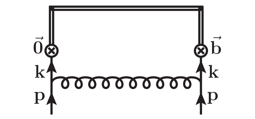
(a) Vertex diagram

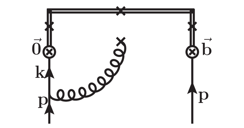
(b) Sail topology

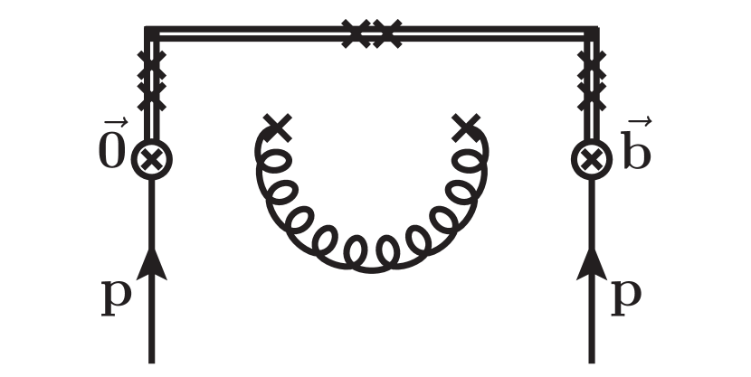
(c) Wilson line self energy

Figure 3: One-loop diagrams contributing to the quasi TMD beam function (with the mirrored sail diagram not shown). The double line represents straight Wilson line segments and the $\otimes$ are the quark fields. The crosses in (b) and (c) denote the set of locations for attaching the gluon that have to be added.

4.1.1 Vertex diagram

The vertex diagram shown in Fig. 3(a) is given by

$$\tilde{q}^{(1)\,\rho\lambda}_{{\rm v}\,,\,\xi}(b,p,\mu,\epsilon) =\frac{1}{2}g^{2}C_{F}\mu_{0}^{2\epsilon}\int\frac{\mathrm{d}^{d}k}{(2\pi)^{d}}e^{\mathrm{i}k\cdot b}\frac{\frac{1}{2}\mathrm{tr}[\gamma^{\rho}\gamma^{\mu}\not{k}\gamma^{\lambda}\not{k}\gamma^{\nu}]}{k^{4}(p-k)^{2}}\biggl{[}\delta_{\mu\nu}-(1-\xi)\frac{(p-k)_{\mu}(p-k)_{\nu}}{(p-k)^{2}}\biggr{]}$$

$$\equiv\frac{\alpha_{s}C_{F}}{4\pi}\Bigl{[}\tilde{q}^{(1)\,\rho\lambda}_{\rm v}(b,p,\mu,\epsilon)+(1-\xi)\Delta\tilde{q}^{(1)\,\rho\lambda}_{\rm v}(b,p,\mu,\epsilon)\Bigr{]}\,.$$ (59)

After evaluating the Dirac trace, the integrals can be expressed in terms of the master integrals defined in eq. (4.1) as

$$\tilde{q}^{(1)\,\rho\lambda}_{\rm v}(b,p,\mu,\epsilon) =(2-2\epsilon)(4\pi\mu_{0}^{\epsilon})^{2}\int\frac{\mathrm{d}^{d}k}{(2\pi)^{d}}e^{\mathrm{i}k\cdot b}\left[\frac{\delta^{\rho\lambda}}{k^{2}(p-k)^{2}}-\frac{2k^{\rho}k^{\lambda}}{k^{4}(p-k)^{2}}\right]$$ (60)

$$=-2\delta^{\rho\lambda}I_{1,1}(b,p)+4I_{2,1}^{\rho\lambda}(b,p)\,,$$

$$\Delta\tilde{q}^{(1)\,\rho\lambda}_{\rm v}(b,p,\mu,\epsilon) =-(4\pi\mu_{0}^{\epsilon})^{2}\int\frac{\mathrm{d}^{d}k}{(2\pi)^{d}}e^{\mathrm{i}k\cdot b}\biggl{[}\frac{\delta^{\rho\lambda}}{k^{2}(p-k)^{2}}-\frac{2k^{\lambda}p^{\rho}}{k^{4}(p-k)^{2}}+\frac{2p^{\lambda}(k^{\rho}-p^{\rho})}{k^{2}(p-k)^{4}}$$

$$\hskip 128.0374pt+\frac{2p^{2}k^{\lambda}(p^{\rho}-k^{\rho})}{k^{4}(p-k)^{4}}\biggr{]}$$

$$=\delta^{\rho\lambda}I_{1,1}(b,p)-2p^{\rho}I_{2,1}^{\lambda}(b,p)+2p^{\lambda}\Bigl{[}I_{1,2}^{\rho}(b,p)-p^{\rho}I_{1,2}(b,p)\Bigr{]}$$

$$\quad+2p^{2}\Bigl{[}p^{\rho}I^{\lambda}_{2,2}(b,p)-I_{2,2}^{\rho\lambda}(b,p)\Bigr{]}\,.$$ (61)

Note that all poles explicitly cancel between the different master integrals, as infrared poles are regulated by the offshellness $p^{2}>0$ and UV poles are regulated by $b^{2}>0$.

4.1.2 Sail diagram

The sail topology of Fig. 3(b) and its mirror diagram are given by

$$\tilde{q}^{(1)\,\rho\lambda}_{{\rm s}\,,\,\xi}(b,p,\mu,\epsilon,L) =-\frac{\mathrm{i}}{2}g^{2}C_{F}\mu_{0}^{2\epsilon}e^{\mathrm{i}{p{\cdot}b}}\int_{0}^{1}\mathrm{d}s\,\gamma^{\prime\mu}(s)\int\frac{\mathrm{d}^{d}k}{(2\pi)^{d}}\biggl{[}\delta^{\mu\nu}-(1-\xi)\frac{k^{\mu}k^{\nu}}{k^{2}}\biggr{]}$$

$$~{}\quad\times\biggl{[}e^{-\mathrm{i}k\cdot\gamma(s)}\frac{\frac{1}{2}\mathrm{tr}[\gamma^{\rho}\gamma^{\lambda}(\not{p}-\not{k})\gamma_{\nu}]}{k^{2}(p-k)^{2}}+e^{\mathrm{i}k\cdot[\gamma(s)-b]}\frac{\frac{1}{2}\mathrm{tr}[\gamma^{\rho}\gamma_{\nu}(\not{p}-\not{k})\gamma^{\lambda}]}{k^{2}(p-k)^{2}}\biggr{]}$$

$$\equiv\frac{\alpha_{s}C_{F}}{4\pi}\Bigl{[}\tilde{q}^{(1)\,\rho\lambda}_{\rm s}(b,p,\mu,\epsilon,L)+(1-\xi)\Delta\tilde{q}^{(1)\,\rho\lambda}_{\rm s}(b,p,\mu,\epsilon,L)\Bigr{]}\,.$$ (62)

For compactness, we parameterize the Wilson lines by a path $\gamma(s)$, such that

$$W_{\gamma} =P\exp\left[-\mathrm{i}g\int_{0}^{1}\mathrm{d}s\,\gamma^{\prime}(s)\cdot\mathcal{A}[\gamma(s)]\right]\,,$$ (63)

where $\gamma^{\prime\mu}(s)=\mathrm{d}\gamma^{\mu}(s)/\mathrm{d}s$ and $\gamma(s)$ is composed of three straight segments given by

$$\gamma_{1}(s) =\left(\begin{matrix}0\\ \vec{0}_{T}\\ Ls\end{matrix}\right)\,,\quad\gamma_{2}(s)=\left(\begin{matrix}0\\ s\vec{b}_{T}\\ L\end{matrix}\right)\,,\quad\gamma_{3}(s)=\left(\begin{matrix}0\\ \vec{b}_{T}\\ L+s(b^{z}-L)\end{matrix}\right)\,,\quad s\in[0,1]\,.$$ (64)

For brevity, here we suppress the explicit dependence of the $\gamma_{i}(s)$ on $b^{\mu}$ and $L$. After evaluating the Dirac trace in eq. (4.1.2), the Feynman gauge piece can be expressed as

$$\tilde{q}^{(1)\,\rho\lambda}_{\rm s}(b,p,\mu,\epsilon,L) =-\mathrm{i}e^{\mathrm{i}{p{\cdot}b}}(4\pi\mu_{0}^{\epsilon})^{2}\int\!\frac{\mathrm{d}^{d}k}{(2\pi)^{d}}\frac{\delta^{\rho\lambda}(p^{\mu}-k^{\mu})-\delta^{\mu\lambda}(p^{\rho}-k^{\rho})+\delta^{\mu\rho}(p^{\lambda}-k^{\lambda})}{k^{2}(p-k)^{2}}$$

$$\hskip 85.35826pt\times\sum_{i=1}^{3}\int_{0}^{1}\mathrm{d}s\,\gamma_{i}^{\prime\mu}(s)\Bigl{(}e^{-\mathrm{i}k\cdot\gamma_{i}(s)}+e^{\mathrm{i}k\cdot[\gamma_{i}(s)-b]}\Bigr{)}\,.$$ (65)

Note that the terms proportional to $\delta^{\mu\lambda}$ and $\delta^{\mu\rho}$ cancel each other in the case $\rho=\lambda$, and that only the term proportional to $k^{\mu}$ yields a $1/\epsilon$ pole, which can easily be extracted since $k\cdot\gamma^{\prime}(s)$ involves a total derivative in $s$. We find

$$\tilde{q}^{(1)\,\rho\lambda}_{\rm s}(b,p,\mu,\epsilon,L) =\delta^{\rho\lambda}e^{\mathrm{i}{p{\cdot}b}}\biggl{[}\frac{2}{\epsilon}-\ln\frac{p^{2}}{\mu^{2}}+4+2I_{1,1}(-b,p)\biggr{]}$$

$$\quad+\mathrm{i}e^{\mathrm{i}{p{\cdot}b}}\sum_{i=1}^{3}\int_{0}^{1}\mathrm{d}s\,\gamma_{i}^{\prime\mu}(s)\Bigl{[}\delta^{\rho\lambda}p^{\mu}\mathbf{\rm I}_{1,1}[-\gamma_{i}(s),p]$$

$$\hskip 128.0374pt-\delta^{\mu\lambda}\bigl{(}p^{\rho}\mathbf{\rm I}_{1,1}[-\gamma_{i}(s),p]-\mathbf{\rm I}_{1,1}^{\rho}[-\gamma_{i}(s),p]\bigr{)}$$

$$\hskip 128.0374pt+\delta^{\mu\rho}\bigl{(}p^{\lambda}\mathbf{\rm I}_{1,1}[-\gamma_{i}(s),p]-\mathbf{\rm I}_{1,1}^{\lambda}[-\gamma_{i}(s),p]\bigr{)}$$

$$\hskip 128.0374pt+\gamma_{i}(s)\to b-\gamma_{i}(s)\Bigr{]}\,,$$ (66)

where we have made the UV pole in $1/\epsilon$ explicit.

In the covariant-gauge piece in eq. (4.1.2), the derivatives of the path always combine to $k\cdot\gamma_{i}(s)$, such that the $\mathrm{d}s$ integration only involves a total derivative, i.e. one only encounters

$$\int_{0}^{1}\mathrm{d}s\,[k\cdot\gamma^{\prime}(s)]e^{\pm\mathrm{i}k\cdot\gamma(s)}=\mp\mathrm{i}\int_{0}^{1}\mathrm{d}s\,\frac{\mathrm{d}}{\mathrm{d}s}e^{\pm\mathrm{i}k\cdot\gamma(s)}=\pm\mathrm{i}\bigl{(}1-e^{\pm\mathrm{i}k\cdot b}\bigr{)}\,.$$ (67)

This gives a simple result in terms of master integrals,

$$\Delta\tilde{q}^{(1)\,\rho\lambda}_{\rm s}(b,p,\mu,\epsilon)$$

$$=-e^{\mathrm{i}{p{\cdot}b}}(4\pi\mu_{0}^{\epsilon})^{2}\int\frac{\mathrm{d}^{d}k}{(2\pi)^{d}}\bigl{(}1-e^{-\mathrm{i}b\cdot k}\bigr{)}\biggl{[}\frac{\delta^{\rho\lambda}}{k^{4}}+\frac{\delta^{\rho\lambda}}{k^{2}(p-k)^{2}}-\frac{\delta^{\rho\lambda}p^{2}}{k^{4}(p-k)^{2}}+2\frac{k^{\lambda}p^{\rho}-k^{\rho}p^{\lambda}}{k^{4}(p-k)^{2}}\biggr{]}$$

$$=\delta^{\rho\lambda}e^{\mathrm{i}{p{\cdot}b}}\Bigl{\{}\bigl{[}\mathbf{\rm I}_{2,0}(p)-\mathbf{\rm I}_{2,0}(-b,p)\bigr{]}+\bigl{[}\mathbf{\rm I}_{1,1}(p)-\mathbf{\rm I}_{1,1}(-b,p)\bigr{]}-p^{2}\bigl{[}\mathbf{\rm I}_{2,1}(p)-\mathbf{\rm I}_{2,1}(-b,p)\bigr{]}\Bigr{\}}$$

$$\quad+2e^{\mathrm{i}{p{\cdot}b}}\Bigl{\{}p^{\rho}\bigl{[}\mathbf{\rm I}_{2,1}^{\lambda}(p)-\mathbf{\rm I}_{2,1}^{\lambda}(-b,p)\bigr{]}-p^{\lambda}\bigl{[}\mathbf{\rm I}_{2,1}^{\rho}(p)-\mathbf{\rm I}_{2,1}^{\rho}(-b,p)\bigr{]}\Bigr{\}}\,.$$ (68)

This result contains a UV pole inducing a logarithmic contribution, given by

$$\Delta\tilde{q}^{(1)\,\rho\lambda}_{\rm s}(b,p,\mu,\epsilon) =\delta^{\rho\lambda}e^{\mathrm{i}{p{\cdot}b}}\left[-\frac{2}{\epsilon}-\ln\frac{\mu^{2}b^{2}}{b_{0}^{2}}-\ln\frac{\mu^{2}}{p^{2}}-2+\mathcal{O}(\epsilon^{0})\right]\,.$$ (69)

Axial projection.

The sail diagram is the only diagram contributing for the axial projector $\mathcal{P}=\frac{1}{2}\gamma^{\rho}\gamma^{5}$. It is obtained similar to eq. (4.1.2) as

$$\tilde{q}^{(1)\,\rho\lambda}_{a\,{\rm s}\,,\,\xi}(b,p,\mu,\epsilon,L) =-\frac{\mathrm{i}}{2}g^{2}C_{F}\mu_{0}^{2\epsilon}e^{\mathrm{i}{p{\cdot}b}}\int_{0}^{1}\mathrm{d}s\,\gamma^{\prime\mu}(s)\int\frac{\mathrm{d}^{d}k}{(2\pi)^{d}}\biggl{[}\delta^{\mu\nu}-(1-\xi)\frac{k^{\mu}k^{\nu}}{k^{2}}\biggr{]}$$

$$~{}\quad\times\biggl{[}e^{-\mathrm{i}k\cdot\gamma(s)}\frac{\frac{1}{2}\mathrm{tr}[\gamma^{\rho}\gamma^{5}\gamma^{\lambda}(\not{p}-\not{k})\gamma_{\nu}]}{k^{2}(p-k)^{2}}+e^{\mathrm{i}k\cdot[\gamma(s)-b]}\frac{\frac{1}{2}\mathrm{tr}[\gamma^{\rho}\gamma^{5}\gamma_{\nu}(\not{p}-\not{k})\gamma^{\lambda}]}{k^{2}(p-k)^{2}}\biggr{]}$$

$$\equiv\frac{\alpha_{s}C_{F}}{4\pi}\Bigl{[}\tilde{q}^{(1)\,\rho\lambda}_{a\,\rm s}(b,p,\mu,\epsilon,L)+(1-\xi)\Delta\tilde{q}^{(1)\,\rho\lambda}_{a\,\rm s}(b,p,\mu,\epsilon,L)\Bigr{]}\,.$$ (70)

The gauge-dependent piece is easily seen to vanish,

$$\Delta\tilde{q}^{(1)\,\rho\lambda}_{a\,\rm s}(b,p,\mu,\epsilon,L)=0\,,$$ (71)

such that only the Feynman piece needs to be considered. The relevant traces are given by

$$\frac{1}{2}\mathrm{tr}[\gamma^{\rho}\gamma^{5}\gamma^{\lambda}(\not{p}-\not{k})\gamma^{\mu}]=-\frac{1}{2}\mathrm{tr}[\gamma^{\rho}\gamma^{5}\gamma^{\mu}(\not{p}-\not{k})\gamma^{\lambda}]=2(k^{\nu}-p^{\nu})\epsilon^{\rho\lambda\nu\mu}\,,$$ (72)

where the antisymmetric tensor is normalized such that $\epsilon^{0123}=1$. Inserting into eq. (4.1.2), we obtain

$$\tilde{q}^{(1)\,\rho\lambda}_{a\,\rm s}(b,p,\mu,\epsilon,L) =\mathrm{i}e^{\mathrm{i}{p{\cdot}b}}\epsilon^{\rho\lambda\nu\mu}\int_{0}^{1}\mathrm{d}s\,\gamma^{\prime\mu}(s)\,(4\pi\mu_{0}^{\epsilon})^{2}\!\!\int\!\!\frac{\mathrm{d}^{d}k}{(2\pi)^{d}}\frac{p^{\nu}-k^{\nu}}{k^{2}(p-k)^{2}}\big{(}e^{-\mathrm{i}k\cdot\gamma(s)}-e^{\mathrm{i}k\cdot[\gamma(s)-b]}\bigr{)}$$

$$=\mathrm{i}e^{\mathrm{i}{p{\cdot}b}}\epsilon^{\rho\lambda\nu\mu}\sum_{i=1}^{3}\int_{0}^{1}\!\!\mathrm{d}s\,\gamma_{i}^{\prime\mu}(s)\Bigl{[}p^{\nu}\bigl{(}\mathbf{\rm I}_{1,1}[\gamma_{i}(s)-b,p]-\mathbf{\rm I}_{1,1}[-\gamma_{i}(s),p]\bigr{)}$$

$$\hskip 136.5733pt-\mathbf{\rm I}^{\nu}_{1,1}[\gamma_{i}(s)-b,p]+\mathbf{\rm I}^{\nu}_{1,1}[-\gamma_{i}(s),p]\Bigr{]}.$$ (73)

Here, the $\mathbf{\rm I}_{1,1}$ are the usual master integrals defined in eq. (4.1). Note that both $\mathbf{\rm I}_{1,1}$ and $\mathbf{\rm I}_{1,1}^{\nu}$ are IR and UV finite, and hence eq. (4.1.2) does not contain any poles in $\epsilon$. In particular, this implies that there is no ambiguity in defining $\gamma^{5}$ in $d=4-2\epsilon$ dimensions for this calculation. The $\gamma_{i}(s)$ in eq. (4.1.2) are the three line segments defined in eq. (64).

4.1.3 Tadpole diagram

The Wilson line self energy, Fig. 3(c), is given by

$$\tilde{q}^{(1)\,\rho\lambda}_{{\rm tp}\,,\,\xi}(b,p,\mu,\epsilon,L) =-\frac{1}{2}\delta^{\rho\lambda}e^{\mathrm{i}b\cdot p}g^{2}C_{F}\mu_{0}^{2\epsilon}\int_{0}^{1}\mathrm{d}s\,\mathrm{d}t\,\gamma^{\prime\mu}(s)\gamma^{\prime\nu}(t)$$

$$\hskip 91.04872pt\times\int\!\!\frac{\mathrm{d}^{d}k}{(2\pi)^{d}}\frac{e^{\mathrm{i}k\cdot[\gamma(t)-\gamma(s)]}}{k^{2}}\biggl{[}\delta^{\mu\nu}-(1-\xi)\frac{k^{\mu}k^{\nu}}{k^{2}}\biggr{]}$$

$$\equiv\frac{\alpha_{s}C_{F}}{4\pi}\Bigl{[}\tilde{q}^{(1)\,\rho\lambda}_{\rm tp}(b,p,\mu,\epsilon,L)+(1-\xi)\Delta\tilde{q}^{(1)\,\rho\lambda}_{\rm tp}(b,p,\mu,\epsilon,L)\Bigr{]}\,,$$ (74)

where as in Sec. 4.1.2 $\gamma(s)$ is the Wilson line path and we included a symmetry factor $1/2$. The Feynman piece can be obtained from ref. Ebert:2019okf ,

$$\tilde{q}^{(1)\,\rho\lambda}_{\rm tp}(b,p,\mu,\epsilon,L)=2\delta^{\rho\lambda}e^{\mathrm{i}b\cdot p}\biggl{[} \frac{3}{\epsilon}+\ln\frac{L^{2}\mu^{2}}{b_{0}^{2}}+\ln\frac{b_{T}^{2}\mu^{2}}{b_{0}^{2}}+\ln\frac{(b^{z}-L)^{2}\mu^{2}}{b_{0}^{2}}+6$$

$$-2\frac{b^{z}}{b_{T}}\arctan\frac{b^{z}}{b_{T}}+2\frac{L}{b_{T}}\arctan\frac{L}{b_{T}}+2\frac{L-b^{z}}{b_{T}}\arctan\frac{L-b^{z}}{b_{T}}$$

$$-\ln\frac{[b_{T}^{2}+L^{2}][b_{T}^{2}+(L-b^{z})^{2}]}{b_{T}^{2}[b_{T}^{2}+(b^{z})^{2}]}\biggr{]}\,.$$ (75)

The covariant piece only involves an integral over a total derivative in $s$, and is given by

$$\Delta\tilde{q}^{(1)\,\rho\lambda}_{\rm tp}(b,p,\mu,\epsilon,L) =\delta^{\rho\lambda}e^{\mathrm{i}b\cdot p}(4\pi\mu_{0}^{\epsilon})^{2}\int\frac{\mathrm{d}^{d}k}{(2\pi)^{d}}\frac{1-e^{\mathrm{i}k\cdot b}}{k^{4}}$$

$$=\delta^{\rho\lambda}e^{\mathrm{i}b\cdot p}\left[\frac{1}{\epsilon}+\ln\frac{b^{2}\mu^{2}}{b_{0}^{2}}+\mathcal{O}(\epsilon)\right]\,.$$ (76)

4.1.4 Full $\mathcal{O}(\alpha_{s})$ result

The full one-loop result for the amputated Green’s function defined in eqs. (52) and (4.1) is given by

$$\tilde{q}^{\rho\lambda}_{\xi}(b,p,\epsilon,L) =\delta^{\rho\lambda}e^{\mathrm{i}{p{\cdot}b}}+\frac{\alpha_{s}(\mu)C_{F}}{4\pi}\tilde{q}^{(1)\,\rho\lambda}_{\xi}(b,p,\mu,\epsilon,L)+\mathcal{O}(\alpha_{s}^{2})\,,$$

$$\tilde{q}^{(1)\,\rho\lambda}_{\xi}(b,p,\mu,\epsilon,L) =\tilde{q}^{\rho\lambda\,(1)}(b,p,\mu,\epsilon,L)+(1-\xi)\,\Delta\tilde{q}^{\rho\lambda\,(1)}(b,p,\mu,\epsilon,L)\,,$$ (77)

where the two pieces are given by

$$\tilde{q}^{\rho\lambda\,(1)}(b,p,\mu,\epsilon,L) =\tilde{q}^{\rho\lambda\,(1)}_{\rm v}(b,p,\mu,\epsilon)+\tilde{q}^{\rho\lambda\,(1)}_{\rm s}(b,p,\mu,\epsilon,L)+\tilde{q}^{\rho\lambda\,(1)}_{\rm tp}(b,p,\mu,\epsilon,L)\,,$$ (78)

$$\Delta\tilde{q}^{\rho\lambda\,(1)}(b,p,\mu,\epsilon) =\Delta\tilde{q}^{\rho\lambda\,(1)}_{\rm v}(b,p,\mu,\epsilon)+\Delta\tilde{q}^{\rho\lambda\,(1)}_{\rm s}(b,p,\mu,\epsilon,L)+\Delta\tilde{q}^{\rho\lambda\,(1)}_{\rm tp}(b,p,\mu,\epsilon,L)\,.$$

The individual pieces can be found in eqs. (60), (4.1.2) and (4.1.3) for $\tilde{q}^{\rho\lambda\,(1)}$, and in eqs. (4.1.1), (4.1.2) and (4.1.3) for $\Delta\tilde{q}^{\rho\lambda\,(1)}$, respectively.

We have checked that the poles in $\epsilon$ agree with those reported in ref. Ebert:2019okf ; Constantinou:2019vyb , and verified numerically that after dropping these poles our result at $b^{z}=0$ agrees with ref. Constantinou:2019vyb . Note that our results are significantly more involved than those in ref. Constantinou:2019vyb because we keep $b^{z}\neq 0$, which is necessary for the quasi-beam function that is needed as input for the calculation of $\gamma_{\zeta}^{q}(\mu,b_{T})$.

For the axial projection, there is only one nonvanishing contribution, such that

$$\tilde{q}^{\rho\lambda}_{a\,\xi}(b,p,\epsilon,L) =\frac{\alpha_{s}(\mu)C_{F}}{4\pi}\tilde{q}^{\rho\lambda\,(1)}_{a\,\rm s}(b,p,\mu,\epsilon,L)+\mathcal{O}(\alpha_{s}^{2})\,,$$ (79)

where $q^{\rho\lambda\,(1)}_{a\,\rm s}$ is given in eq. (4.1.2).

4.2 RI^′/MOM renormalization factor and conversion to ${\overline{\mathrm{MS}}}$

Having calculated the full one-loop result for the off-shell amputated Green’s function $\tilde{q}^{\rho\lambda}$, we can now proceed to calculate the RI^′/MOM renormalization and the conversion to the ${\overline{\mathrm{MS}}}$ scheme. This also requires the one-loop wave function renormalization to account for the external state in the amputated Green’s function. In the RI^′/MOM scheme it is given by Martinelli:1994ty

$$Z_{\rm wf}^{-1}(p,\epsilon) =\frac{1}{4p^{2}}\mathrm{Tr}\bigl{[}S^{-1}(p)\not{p}\bigr{]}=1-\frac{\alpha_{s}(\mu)C_{F}}{4\pi}Z_{\rm wf}^{(1)}(p,\mu,\epsilon)+\mathcal{O}(\alpha_{s}^{2})\,,$$

$$Z_{\rm wf}^{(1)}(p,\mu,\epsilon) =-[1-(1-\xi)]\Bigl{(}\frac{1}{\epsilon}+\ln\frac{\mu^{2}}{p^{2}}+1\Bigr{)}\,.$$ (80)

The RI^′/MOM renormalization of the quasi-TMDPDF also requires us to include the one-loop soft factor. Using eq. (16), it can be written as

$$\tilde{\Delta}_{S}^{q}(b_{T},\epsilon,L) =\frac{1}{\sqrt{\tilde{S}^{q}_{\rm bent}(b_{T},\epsilon,L)}}=1-\frac{1}{2}\frac{\alpha_{s}(\mu)C_{F}}{4\pi}\tilde{S}^{q\,(1)}_{\rm bent}(b_{T},\mu,\epsilon,L)\,.$$ (81)

The required one-loop result for the bent soft function can be obtained from ref. Ebert:2019okf as

$$\tilde{S}^{q\,(1)}_{\rm bent}(b_{T},\mu,\epsilon,L) =\frac{12}{\epsilon}+12\ln\frac{\mu^{2}b_{T}^{2}}{b_{0}^{2}}+16\frac{L}{b_{T}}\arctan\frac{L}{b_{T}}+24$$

$$\quad+4\sqrt{2}\frac{b_{T}}{L}\arctan\frac{b_{T}}{\sqrt{2}L}-4\ln\frac{b_{T}^{2}+2L^{2}}{2L^{2}}-8\ln\frac{b_{T}^{2}+L^{2}}{L^{2}}\,.$$ (82)

The RI^′/MOM to ${\overline{\mathrm{MS}}}$ conversion kernel follows from eqs. (43), (44) and (3) as

$$\tilde{Z}_{q}^{\prime\rho\lambda}(b^{z},\mu,b_{T}^{R},p_{R},L) =\lim_{\epsilon\to 0}\frac{\tilde{Z}_{q}^{\overline{\mathrm{MS}}}(\mu,\epsilon)Z_{\rm wf}(p_{R},\epsilon)\tilde{q}^{\rho\lambda}_{\xi}(b^{z},b_{T}^{R},p_{R},\epsilon,L)\tilde{\Delta}_{S}^{q}(b_{T}^{R},\epsilon,L)}{\tilde{q}^{(0)\,\rho\lambda}_{\xi}(b^{z},b_{T}^{R},p_{R})}$$

$$=1+\frac{\alpha_{s}(\mu)C_{F}}{4\pi}\Bigl{[}e^{-\mathrm{i}\vec{b}_{T}^{R}\cdot\vec{p}_{T}^{R}-\mathrm{i}b^{z}p^{z}}\,\tilde{q}^{\rho\lambda~{}(1)}_{\xi}(b^{z},b_{T}^{R},p_{R},\mu,\epsilon,L)+Z_{\rm wf}^{(1)}(p_{R},\mu,\epsilon)$$

$$\hskip 85.35826pt-\frac{1}{2}\tilde{S}^{q\,(1)}_{\rm bent}(b_{T}^{R},\mu,\epsilon,L)\Bigr{]}_{\mathcal{O}(\epsilon^{0})}+\mathcal{O}(\alpha_{s}^{2})\,,$$ (83)

where all the $1/\epsilon$ poles are canceled by $\tilde{Z}_{q}^{\overline{\mathrm{MS}}}(\mu,\epsilon)$, so only the $\mathcal{O}(\epsilon^{0})$ terms are extracted from the terms in the square brackets.

Last but not least, one may note that $\tilde{\Delta}_{S}^{q}(b_{T}^{R},\epsilon,L)$ also formally cancels out in the ratios in eqs. (22) and (29) due to its $b^{z}$-independence, and therefore equivalently we can drop it in eq. (4.2) and obtain the conversion factor that matches the RI^′/MOM-renormalized quasi-beam function to the ${\overline{\mathrm{MS}}}$ scheme,

$$\tilde{Z}_{B}^{\prime\rho\lambda}(b^{z},\mu,b_{T}^{R},p_{R},L)=1+\frac{\alpha_{s}(\mu)C_{F}}{4\pi}\Bigl{[} e^{-\mathrm{i}\vec{b}_{T}^{R}\cdot\vec{p}_{T}^{R}-\mathrm{i}b^{z}p^{z}}\,\tilde{q}^{\rho\lambda~{}(1)}_{\xi}(b^{z},b_{T}^{R},p_{R},\mu,\epsilon,L)$$

$$+Z_{\rm wf}^{(1)}(p_{R},\mu,\epsilon)\Bigr{]}_{\mathcal{O}(\epsilon^{0})}+\mathcal{O}(\alpha_{s}^{2})\,.$$ (84)

However, this $\tilde{Z}_{B}^{\prime}$ will suffer from $L/b_{T}$ divergence that makes its numerical value much larger than one, indicating that the perturbation series does not converge. In constrast, $\tilde{Z}_{q}^{\prime}$ in eq. (4.2), which includes the correction from $\tilde{\Delta}_{S}^{q}$, is free from such divergences and has good perturbative convergence, as we will demonstrate numerically in the following section.

5 Numerical results

In this section, we numerically illustrate the importance of the perturbative matching from the RI^′/MOM to the ${\overline{\mathrm{MS}}}$ scheme. We assume a lattice with spacing $a=0.06~{}\mathrm{fm}$ and size $L_{\rm lat}=32\,a$, and set the length of the Wilson line to $L=10\,a$. The ${\overline{\mathrm{MS}}}$ renormalization scale is chosen as $\mu=3~{}\mathrm{GeV}$, with $\alpha_{s}(\mu)=0.2492$ obtained using three-loop running from $\alpha_{s}(m_{Z})=0.118$. We always work in Landau gauge with $\xi=0$. To show the effect of canceling linear divergences in $L/b_{T}$, we will consider both the conversion factor $\tilde{Z}_{q}^{\prime}$ for the quasi-TMDPDF and $\tilde{Z}_{B}^{\prime}$ for the quasi-beam function alone.

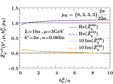
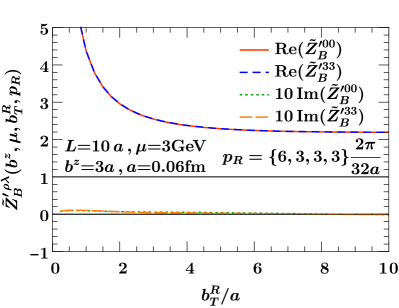
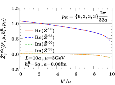
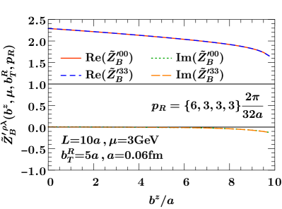
Figure 4: One-loop conversion factors $\tilde{Z}^{\prime}$ from the RI^′/MOM scheme to the ${\overline{\mathrm{MS}}}$ scheme for the quasi-TMDPDF (left) and the quasi-beam function (right), as a function of $b_{T}/a$ for $b^{z}=0$ (top), as a function of $b_{T}/a$ for $b^{z}=3\,a$ (middle) and as a function of $b^{z}/a$ for $b_{T}=5\,a$ (bottom).

We first consider the Euclidean momentum

$$p_{R}^{\mu} =(p_{R}^{0},\vec{p}_{R}\,)=(6,3,3,3)\frac{2\pi}{L_{\rm lat}}\,\approx(3.9,1.9,1.9,1.0)~{}\mathrm{GeV}\,,$$

$$p_{R}^{2} =(p_{R}^{0})^{2}+{\vec{p}}_{R}^{\,2}=63\Bigl{(}\frac{2\pi}{L_{\rm lat}}\Bigr{)}^{2}\approx(5.1~{}\mathrm{GeV})^{2}\,.$$ (85)

In Fig. 4, we show $\tilde{Z}_{q}^{\prime}$ in the left panel and $\tilde{Z}_{B}^{\prime}$ in the right panel. The $b_{T}$ dependence is shown for fixed $b^{z}=0$ (top row) and $b^{z}=3a$ (middle row), while the bottom row shows the $b^{z}$ dependence for fixed $b_{T}=5a$. In each plot, we show real and imaginary parts for the $\rho=\lambda=0$ Dirac structure in solid red and dotted green, respectively, as well as the real and imaginary parts for $\rho=\lambda=3$ in dashed blue and dashed orange, respectively. The imaginary parts in the first two rows are amplified by a factor of ten to increase their visibility. The off-diagonal Dirac structures with $\rho\neq\lambda$ are very small and not shown here. In all cases, we find a very small imaginary part of both $Z_{B}^{\prime}$ and $Z_{q}^{\prime}$, and that the two choices $\lambda=\rho=0$ and $\lambda=\rho=3$ are very similar. Hence in the following, we restrict our discussion to the real part and the choice $\rho=\lambda=0$ only.

For $\tilde{Z}_{B}^{\prime}$ (right panels of Fig. 4), the presence of the $L/b_{T}^{R}$ divergence is clearly visible, and leads to large values for this factor. Since this coefficient is $1$ at lowest order, clearly perturbation theory is not converging for $\tilde{Z}_{B}^{\prime}$, as anticipated.

For $\tilde{Z}_{q}^{\prime}$ (left panels of Fig. 4), we generically observe corrections close to $Z_{q}^{\prime}=1$, indicating that the $\mathcal{O}(\alpha_{s})$ corrections are rather moderate and of the expected size of a NLO correction. However, there is a significant dependence on both $b_{T}^{R}$ and $b^{z}$. In particular, one can observe a mild logarithmic dependence on $b_{T}^{R}$ as $b_{T}^{R}\to 0$. Since $b_{T}^{R}$ is a free parameter in the renormalization procedure, one can choose it freely to yield small matching corrections, as long as $b_{T}^{R}$ is perturbative. The results in Fig. 4 indicate that $b_{T}^{R}\gtrsim a$ is a good choice. In order to minimize lattice discretization effects, which are not captured in our analytic calculation, one must choose $b_{T}^{R}\gg a$, so in practice we expect that $b_{T}^{R}\sim\mathcal{O}(\mathrm{few}~{}a)$ is a reasonable choice. There is also a significant $b^{z}$ dependence, arising from the fact that in the RI^′/MOM scheme one fully absorbs the $b^{z}$-dependence at $p=p_{R}$ and $b_{T}=b_{T}^{R}$ into the UV renormalization, and this $b^{z}$ dependence must therefore be corrected perturbatively through the conversion to the ${\overline{\mathrm{MS}}}$ scheme.

For larger $b^{z}$ the correction from $\tilde{Z}_{q}^{\prime}$ becomes numerically significant, as can seen from the bottom left panel of Fig. 4. The impact of this large $b^{z}$ region is suppressed by the large parton momentum when the quasi-TMDPDF is Fourier transformed into the $x$-space, namely through the oscillation caused by the Fourier exponents involving $(xP^{z}b^{z})$ in eq. (22). For the position space version in eq. (29) the analogous suppression of the large $b^{z}$ region occurs from the falling and oscillating behavior of $\bar{C}_{\rm ns}$ with $(P^{z}b^{z})$. The derivation of eq. (2.3), and thus both the momentum and position space formulae for $\gamma_{\zeta}^{q}$, assume the hierarchy $b^{z}\ll L$, and hence dominance of the integral away from the large $b^{z}\sim L$ region. Studying numerically the dependence of eqs. (22) and (29) on the upper limit of $b^{z}$ used in the integrations will help us understand how well this hierarchy is obeyed.

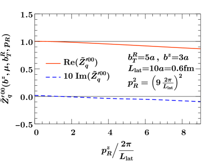
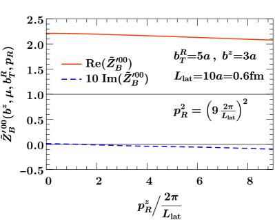
Figure 5: One-loop conversion factors $\tilde{Z}^{\prime}$ from the RI^′/MOM scheme to the ${\overline{\mathrm{MS}}}$ scheme for the quasi-TMDPDF (left) and the quasi-beam function (right), as a function of the $z$ momentum, $p_{R}^{z}$, of the quark state.

Finally, we study the $p_{R}^{z}$ dependence for fixed $b_{T}=5\,a$ and $b^{z}=3\,a$. For a given $p_{R}^{z}$ there is still considerable freedom for the other parameters of $p_{R}$, and we choose the Euclidean momentum

$$p_{R}^{\mu}=\bigl{(}\sqrt{79-(p_{R}^{z})^{2}},1,1,p_{R}^{z}\bigr{)}\frac{2\pi}{L_{\rm lat}}\,,\quad p_{R}^{2}=\Bigl{(}9\frac{2\pi}{L_{\rm lat}}\Bigr{)}^{2}\approx(5.8~{}\mathrm{GeV})^{2}\,,$$ (86)

where $p_{R}^{0}$ is a function of $p_{R}^{z}$ such that $p_{R}^{2}$ is fixed. The largest value of $p_{R}^{z}$ yielding a real solution for $p_{R}^{0}$ is then given by $p_{R}^{z}=\sqrt{79}(2\pi/L_{\rm lat})\approx 5.7~{}\mathrm{GeV}$. Fig. 5 shows the resulting scheme conversion factors, with $\tilde{Z}_{q}^{\prime}$ on the left and $\tilde{Z}_{B}^{\prime}$ on the right. As before, in both cases the imaginary part (blue dashed) is very small, and the real part (red) is close to unity for $\tilde{Z}_{q}^{\prime}$ indicating that perturbation theory is working as expected, while it has significant deviation from unity for $\tilde{Z}_{B}^{\prime}$ (where we see that perturbation theory is breaking down). For $\tilde{Z}_{q}^{\prime}$ it can also be observed that there is a relatively mild dependence on $p_{R}^{z}$.

6 Conclusion

In this paper we have elaborated on the method to determine the Collins-Soper kernel using ratios of quasi-TMDPDFs. Originally, in ref. Ebert:2018gzl a method was proposed which used ratios of properly matched and renormalized quasi-TMDPDFs in momentum space. This requires a Fourier transformation of spatial correlations obtained from the lattice to momentum space, which can be numerically challenging. Here we have extended this proposal to demonstrate how to carry out the matching for renormalized ratios directly in position space. This trades the Fourier transformation for a convolution with a position space matching coefficient, which we expect will improve the numerical stability of the method. The required position space matching coefficient $\bar{C}_{\rm ns}(\mu,y,P^{z})$ was obtained here at ${\cal O}(\alpha_{s})$.

In addition, we have calculated a renormalization scheme conversion factor that is needed for the lattice calculation. Renormalization on the lattice must necessarily be done nonperturbatively to properly handle power law divergences from spatial Wilson line self energies. Here we calculated the one-loop renormalization factor for the transverse-momentum dependent quasi-TMDPDFs in the regularization-independent momentum subtraction RI^′/MOM scheme with $b^{z}\neq 0$, and used this result to obtain the one-loop conversion factor $\tilde{Z}_{q}^{\prime}(b^{z},\mu,\tilde{\mu})$ that converts from the RI^′/MOM scheme to the ${\overline{\mathrm{MS}}}$ scheme. This conversion factor is necessary to obtain results for the Collins-Soper kernel $\gamma_{\zeta}^{q}(\mu,b_{T})$ in the desired ${\overline{\mathrm{MS}}}$ scheme. Our results are thus key to determining the Collins-Soper kernel from lattice QCD using ratios of quasi-TMDPDFs as proposed in ref. Ebert:2018gzl , and elaborated on in ref. Ebert:2019okf . These results will also be used in the lattice study of nonperturbative renormalization of the quasi-beam functions Shanahan:2019zcq .

Together the results obtained here provide important ingredients to enable a first nonperturbative determination of the Collins-Soper kernel from lattice QCD.

Appendix A Master integrals

The master integrals required in Sec. 4 were defined in eq. (4.1) as

$$\mathbf{\rm I}_{i,j}^{\mu\nu\cdots}(b,p) =-(4\pi\mu_{0}^{\epsilon})^{2}\int\!\frac{\mathrm{d}^{d}k}{(2\pi)^{d}}\frac{k^{\mu}k^{\nu}\cdots}{(k^{2})^{i}[(p-k)^{2}]^{j}}\,e^{\mathrm{i}k\cdot b}\,,$$

$$\mathbf{\rm I}_{i,j}^{\mu\nu\cdots}(p) =-(4\pi\mu_{0}^{\epsilon})^{2}\int\!\frac{\mathrm{d}^{d}k}{(2\pi)^{d}}\frac{k^{\mu}k^{\nu}\cdots}{(k^{2})^{i}[(p-k)^{2}]^{j}}\,,$$ (87)

where we employ a Euclidean metric. All required tensor structures can be obtained from the scalar integrals through

$$\mathbf{\rm I}_{i,j}^{\mu}(p) =\frac{p^{\mu}}{2}\biggl{[}I_{i,j}(p)+\frac{1}{p^{2}}I_{i-1,j}(p)-\frac{1}{p^{2}}I_{i,j-1}(p)\biggr{]}\,,$$ (88)

$$\mathbf{\rm I}_{i,j}^{\mu}(b,p) =-2\mathrm{i}b^{\mu}\frac{\partial\mathbf{\rm I}_{i,j}(b,p)}{\partial(b^{2})}-\mathrm{i}p^{\mu}\frac{\partial\mathbf{\rm I}_{i,j}(b,p)}{\partial({p{\cdot}b})}\,,$$

$$\mathbf{\rm I}_{i,j}^{\mu\nu}(b,p) =-2\delta^{\mu\nu}\frac{\partial\mathbf{\rm I}_{i,j}}{\partial(b^{2})}-2(p^{\mu}b^{\nu}+b^{\mu}p^{\nu})\frac{\partial^{2}\mathbf{\rm I}_{i,j}}{\partial(b^{2})\partial({p{\cdot}b})}-4b^{\mu}b^{\nu}\frac{\partial^{2}\mathbf{\rm I}_{i,j}}{\partial^{2}(b^{2})}-p^{\mu}p^{\nu}\frac{\partial^{2}\mathbf{\rm I}_{i,j}}{\partial^{2}({p{\cdot}b})}\,.$$

Here, we employed that $I_{i,j}(b,p)$ can only depend on the Lorentz scalars $b^{2}$, ${p{\cdot}b}$ and $p^{2}$, and for brevity suppressed the arguments in the last line of eq. (88).

The scalar integrals $I_{i,j}(b,p)$ and $I_{i,j}(p)$ can be evaluated using Feynman parameters and standard integral techniques. In the Euclidean regime, we have $b^{2}>0$ and $p^{2}>0$, which yields the general results

$$\mathbf{\rm I}_{i,j}(p) =-(p^{2})^{2-i-j}\left(\frac{\mu^{2}e^{\gamma_{E}}}{p^{2}}\right)^{\epsilon}\frac{\Gamma(i+j+\epsilon-2)}{\Gamma(4-i-j-2\epsilon)}\frac{\Gamma(2-i-\epsilon)}{\Gamma(i)}\frac{\Gamma(2-j-\epsilon)}{\Gamma(j)}\,,$$ (89)

$$\mathbf{\rm I}_{i,j}(b,p) =-\frac{2(\mu^{2}e^{\gamma_{E}})^{\epsilon}}{\Gamma(i)\Gamma(j)}\biggl{(}\frac{4p^{2}}{b^{2}}\biggr{)}^{1-(i+j+\epsilon)/2}$$

$$\quad\times\int_{0}^{1}\mathrm{d}x\,x^{(j-i-\epsilon)/2}(1-x)^{(i-j-\epsilon)/2}e^{\mathrm{i}x{p{\cdot}b}}K_{i+j+\epsilon-2}\bigl{(}\sqrt{b^{2}p^{2}x(1-x)}\bigr{)}\,.$$ (90)

Here, $K_{n}(z)$ is the modified Bessel function of second kind.

The results in eqs. (89) and (A) contain divergences as $\epsilon\to 0$, which typically cancel in the expressions for the individual diagrams given in Sec. 4, so that one can let $\epsilon\to 0$ right away. This cancellation can also be made manifest by extracting the explicit poles in $1/\epsilon$. For the scalar integrals in eq. (89), expanding in $\epsilon$ gives

$$I_{0,j}(p)=I_{i,0}(p) =0\,,$$

$$I_{1,1}(p) =-\frac{1}{\epsilon}-\ln\frac{\mu^{2}}{p^{2}}-2+\mathcal{O}(\epsilon)\,,$$

$$I_{1,2}(p)=I_{2,1}(p) =\frac{1}{p^{2}}\left[\frac{1}{\epsilon}+\ln\frac{\mu^{2}}{p^{2}}+\mathcal{O}(\epsilon)\right]\,,$$

$$I_{2,2}(p) =\frac{2}{(p^{2})^{2}}\left[\frac{1}{\epsilon}+\ln\frac{\mu^{2}}{p^{2}}+1+\mathcal{O}(\epsilon)\right]\,.$$ (91)

The integral over the Feynman parameter $x$ in eq. (A) is not known for arbitrary parameters $i$ and $j$, and has to be evaluated numerically. Infrared divergences as $x\to 0$ to $x\to 1$ can be extracted using the asymptotic limit of $K_{n}(z\to 0)$,

$$\mathbf{\rm I}_{2,0}(b,p) =\frac{1}{\epsilon}+\ln\frac{b^{2}\mu^{2}}{b_{0}^{2}}$$

$$\mathbf{\rm I}_{1,1}(b,p) = \int_{0}^{1}\mathrm{d}x\,\mathcal{I}_{1,1}(x,b^{2},{p{\cdot}b},p^{2})$$

$$\mathbf{\rm I}_{1,2}(b,p) =\frac{e^{\mathrm{i}{p{\cdot}b}}}{p^{2}}\biggl{[}\frac{1}{\epsilon}+\ln\frac{\mu^{2}}{p^{2}}\biggr{]} +\int_{0}^{1}\mathrm{d}x\,\mathcal{I}_{1,2}(x,b^{2},{p{\cdot}b},p^{2})$$

$$\mathbf{\rm I}_{2,1}(b,p) =\frac{1}{p^{2}}\biggl{[}\frac{1}{\epsilon}+\ln\frac{\mu^{2}}{p^{2}}\biggr{]} +\int_{0}^{1}\mathrm{d}x\,\mathcal{I}_{2,1}(x,b^{2},{p{\cdot}b},p^{2})$$

$$\mathbf{\rm I}_{2,2}(b,p) =\frac{1+e^{\mathrm{i}{p{\cdot}b}}}{p^{4}}\biggl{[}\frac{1}{\epsilon}+\ln\frac{\mu^{2}}{p^{2}}+1\biggr{]} +\int_{0}^{1}\mathrm{d}x\,\mathcal{I}_{2,2}(x,b^{2},{p{\cdot}b},p^{2})\,,$$ (92)

where the integral kernels are defined as

$$\mathcal{I}_{1,1}(x,b^{2},{p{\cdot}b},p^{2}) =-2e^{\mathrm{i}x{p{\cdot}b}}K_{0}\Bigl{(}\sqrt{b^{2}p^{2}x(1-x)}\Bigr{)}$$

$$\tilde{\mathcal{I}}_{1,2}(x,b^{2},{p{\cdot}b},p^{2}) =-\frac{e^{\mathrm{i}{p{\cdot}b}}}{p^{2}}\frac{1}{x}\left[e^{-\mathrm{i}x{p{\cdot}b}}\sqrt{b^{2}p^{2}x(1-x)}K_{1}\Bigl{(}\sqrt{b^{2}p^{2}x(1-x)}\Bigr{)}-1\right]$$

$$\mathcal{I}_{2,1}(x,b^{2},{p{\cdot}b},p^{2}) =-\frac{1}{p^{2}}\frac{1}{x}\left[e^{+\mathrm{i}x{p{\cdot}b}}\sqrt{b^{2}p^{2}x(1-x)}K_{1}\Bigl{(}\sqrt{b^{2}p^{2}x(1-x)}\Bigr{)}-1\right]$$

$$\mathcal{I}_{2,2}(x,b^{2},{p{\cdot}b},p^{2}) =-\frac{1+e^{\mathrm{i}{p{\cdot}b}}}{4p^{4}}\frac{1}{x(1-x)}$$

$$\quad\times\biggl{[}\frac{e^{\mathrm{i}x{p{\cdot}b}}+e^{\mathrm{i}(1-x){p{\cdot}b}}}{1+e^{\mathrm{i}{p{\cdot}b}}}b^{2}p^{2}x(1-x)K_{2}\Bigl{(}\sqrt{b^{2}p^{2}x(1-x)}\Bigr{)}-2\biggr{]}\,.$$ (93)

Appendix B Alternative determination of $\gamma_{\zeta}$ in position space

Here, we present a slightly modified method compared to that presented in Sec. 2.4 for determining $\gamma_{\zeta}$ in position space. There, the Fourier transform of the inverse of the kernel $C_{\rm ns}$ was employed. Here, we directly Fourier transform the kernel $C_{\rm ns}$,

$$C_{\rm ns}(\mu,xP^{z}_{i}) =\int\frac{\mathrm{d}(b^{z}_{i}P^{z}_{i})}{2\pi}\,e^{\mathrm{i}x(b^{z}_{i}P^{z}_{i})}\,\bar{C}_{\rm ns}^{\prime}(\mu,b^{z}_{i}P^{z}_{i},P^{z}_{i})\,,$$

$$\bar{C}_{\rm ns}^{\prime}(\mu,b^{z}_{i}P^{z}_{i},P^{z}_{i}) =\int\!\mathrm{d}x\,e^{-\mathrm{i}x(b^{z}_{i}P^{z}_{i})}\,C_{\rm ns}(\mu,xP^{z}_{i})\,.$$ (94)

As before, we Fourier transform with respect to $b^{z}_{i}P^{z}_{i}$ to absorb superfluous factors of $P^{z}_{i}$.

Plugging eqs. (24) and (B) into eq. (19), we get

$$P^{z}_{2}\int\!\mathrm{d}b^{z}_{1}\,\mathrm{d}b^{z}_{2}\,e^{\mathrm{i}x(b^{z}_{1}P^{z}_{1}+b^{z}_{2}P^{z}_{2})}\bar{C}_{\rm ns}^{\prime}(\mu,b^{z}_{2}P^{z}_{2},P^{z}_{2})\tilde{f}_{\rm ns}(b^{z}_{1},\vec{b}_{T},\mu,P^{z}_{1})$$ (95)

$$=~{} P^{z}_{1}\int\!\mathrm{d}b^{z}_{1}\,\mathrm{d}b^{z}_{2}\,e^{\mathrm{i}x(b^{z}_{1}P^{z}_{1}+b^{z}_{2}P^{z}_{2})}\bar{C}_{\rm ns}^{\prime}(\mu,b^{z}_{1}P^{z}_{1},P^{z}_{1})\tilde{f}_{\rm ns}(b^{z}_{2},\vec{b}_{T},\mu,P^{z}_{2})\ \exp\biggl{[}\gamma_{\zeta}^{q}(\mu,b_{T})\ln\frac{P^{z}_{1}}{P^{z}_{2}}\biggr{]}\,.$$

Next, we Fourier transform both sides from $x$ to $y$ by integrating over $x$ against $e^{-\mathrm{i}xy}$, obtaining

$$\int\!\mathrm{d}b^{z}_{1}\,\bar{C}_{\rm ns}^{\prime}(\mu,y-b^{z}_{1}P^{z}_{1},P^{z}_{2})\tilde{f}_{\rm ns}(b^{z}_{1},\vec{b}_{T},\mu,P^{z}_{1})$$ (96)

$$=~{} \int\!\mathrm{d}b^{z}_{2}\,\bar{C}_{\rm ns}^{\prime}(\mu,y-b^{z}_{2}P^{z}_{2},P^{z}_{1})\tilde{f}_{\rm ns}(b^{z}_{2},\vec{b}_{T},\mu,P^{z}_{2})\times\exp\biggl{[}\gamma_{\zeta}^{q}(\mu,b_{T})\ln\frac{P^{z}_{1}}{P^{z}_{2}}\biggr{]}\,.$$

This can trivially be solved for $\gamma_{\zeta}^{q}$ as

$$\gamma_{\zeta}^{q}(\mu,b_{T}) =\frac{1}{\ln(P^{z}_{1}/P^{z}_{2})}\ln\frac{\int\!\mathrm{d}b^{z}\,\bar{C}_{\rm ns}^{\prime}(\mu,y-b^{z}P^{z}_{1},P^{z}_{2})\tilde{f}_{\rm ns}(b^{z},\vec{b}_{T},\mu,P^{z}_{1})}{\int\!\mathrm{d}b^{z}\,\bar{C}_{\rm ns}^{\prime}(\mu,y-b^{z}P^{z}_{2},P^{z}_{1})\tilde{f}_{\rm ns}(b^{z},\vec{b}_{T},\mu,P^{z}_{2})}\,.$$ (97)

Using the expression eq. (2.2) for $\tilde{f}_{\rm ns}$ and inserting a factor ${\tilde{R}}_{B}$ to separately cancel divergences in $b_{T}/a$, $L/a$ and $L/b_{T}$ in numerator and denominator, we obtain the final expression

$$\gamma_{\zeta}^{q}(\mu,b_{T})=\frac{1}{\ln(P^{z}_{1}/P^{z}_{2})}$$ (98)

$$\times\ln\frac{\int\!\mathrm{d}b^{z}\,\bar{C}_{\rm ns}^{\prime}(\mu,y-b^{z}P^{z}_{1},P^{z}_{2})\tilde{Z}^{\prime}_{q}(b^{z},\mu,\tilde{\mu})\,\tilde{Z}_{\rm uv}^{q}(b^{z},\tilde{\mu},a)\,{\tilde{R}}_{B}(b_{T},\tilde{\mu},a,L)\,\tilde{B}_{\rm ns}(b^{z},\vec{b}_{T},a,P^{z}_{1},L)}{\int\!\mathrm{d}b^{z}\,\bar{C}_{\rm ns}^{\prime}(\mu,y-b^{z}P^{z}_{2},P^{z}_{1})\tilde{Z}^{\prime}_{q}(b^{z},\mu,\tilde{\mu})\,\tilde{Z}_{\rm uv}^{q}(b^{z},\tilde{\mu},a)\,{\tilde{R}}_{B}(b_{T},\tilde{\mu},a,L)\,\tilde{B}_{\rm ns}(b^{z},\vec{b}_{T},a,P^{z}_{2},L)}\,.$$

The key difference to eq. (29) is that in eq. (98), both numerator and denominator depend on $P^{z}_{1}$ and $P^{z}_{2}$, since $\bar{C}_{\rm ns}^{\prime}$ depends on both momenta. In contrast, in eq. (29) the numerator only depends on $P^{z}_{1}$ and the denominator only depends on $P^{z}_{2}$, which makes the bookkeeping simpler for an analysis that separately determines the numerator and denominator before taking ratios.

References

- (1) D. Boer et al., Gluons and the quark sea at high energies: Distributions, polarization, tomography, 1108.1713.
- (2) A. Accardi et al., Electron Ion Collider: The Next QCD Frontier, Eur. Phys. J. A52 (2016) 268 [1212.1701].
- (3) CDF collaboration, T. Affolder et al., The transverse momentum and total cross section of pairs in the boson region from collisions at TeV, Phys. Rev. Lett. 84 (2000) 845 [hep-ex/0001021].
- (4) D0 collaboration, B. Abbott et al., Differential production cross section of bosons as a function of transverse momentum at TeV, Phys. Rev. Lett. 84 (2000) 2792 [hep-ex/9909020].
- (5) D0 collaboration, V. M. Abazov et al., Measurement of the shape of the boson transverse momentum distribution in events produced at TeV, Phys. Rev. Lett. 100 (2008) 102002 [0712.0803].
- (6) D0 collaboration, V. M. Abazov et al., Measurement of the normalized transverse momentum distribution in collisions at TeV, Phys. Lett. B693 (2010) 522 [1006.0618].
- (7) ATLAS collaboration, G. Aad et al., Measurement of the transverse momentum distribution of bosons in proton–proton collisions at =7 TeV with the ATLAS detector, Phys. Lett. B705 (2011) 415 [1107.2381].
- (8) CMS collaboration, S. Chatrchyan et al., Measurement of the Rapidity and Transverse Momentum Distributions of Bosons in Collisions at TeV, Phys. Rev. D85 (2012) 032002 [1110.4973].
- (9) ATLAS collaboration, G. Aad et al., Measurement of the boson transverse momentum distribution in collisions at = 7 TeV with the ATLAS detector, JHEP 09 (2014) 145 [1406.3660].
- (10) CMS collaboration, V. Khachatryan et al., Measurement of the Z boson differential cross section in transverse momentum and rapidity in proton–proton collisions at 8 TeV, Phys. Lett. B749 (2015) 187 [1504.03511].
- (11) ATLAS collaboration, G. Aad et al., Measurement of the transverse momentum and distributions of Drell–Yan lepton pairs in proton–proton collisions at TeV with the ATLAS detector, Eur. Phys. J. C76 (2016) 291 [1512.02192].
- (12) CMS collaboration, V. Khachatryan et al., Measurement of the transverse momentum spectra of weak vector bosons produced in proton-proton collisions at TeV, JHEP 02 (2017) 096 [1606.05864].
- (13) European Muon collaboration, J. Ashman et al., Forward produced hadrons in and scattering and investigation of the charge structure of the nucleon, Z. Phys. C52 (1991) 361.
- (14) ZEUS collaboration, M. Derrick et al., Inclusive charged particle distributions in deep inelastic scattering events at HERA, Z. Phys. C70 (1996) 1 [hep-ex/9511010].
- (15) H1 collaboration, C. Adloff et al., Measurement of charged particle transverse momentum spectra in deep inelastic scattering, Nucl. Phys. B485 (1997) 3 [hep-ex/9610006].
- (16) H1 collaboration, F. D. Aaron et al., Measurement of the Proton Structure Function at Low , Phys. Lett. B665 (2008) 139 [0805.2809].
- (17) HERMES collaboration, A. Airapetian et al., Multiplicities of charged pions and kaons from semi-inclusive deep-inelastic scattering by the proton and the deuteron, Phys. Rev. D87 (2013) 074029 [1212.5407].
- (18) COMPASS collaboration, C. Adolph et al., Hadron Transverse Momentum Distributions in Muon Deep Inelastic Scattering at 160 GeV/, Eur. Phys. J. C73 (2013) 2531 [1305.7317].
- (19) COMPASS collaboration, M. Aghasyan et al., Transverse-momentum-dependent Multiplicities of Charged Hadrons in Muon-Deuteron Deep Inelastic Scattering, Phys. Rev. D97 (2018) 032006 [1709.07374].
- (20) S. Catani and M. Grazzini, Higgs Boson Production at Hadron Colliders: Hard-Collinear Coefficients at the NNLO, Eur. Phys. J. C72 (2012) 2013 [1106.4652].
- (21) S. Catani, L. Cieri, D. de Florian, G. Ferrera and M. Grazzini, Vector boson production at hadron colliders: hard-collinear coefficients at the NNLO, Eur. Phys. J. C72 (2012) 2195 [1209.0158].
- (22) T. Gehrmann, T. Luebbert and L. L. Yang, Calculation of the transverse parton distribution functions at next-to-next-to-leading order, JHEP 06 (2014) 155 [1403.6451].
- (23) T. Lübbert, J. Oredsson and M. Stahlhofen, Rapidity renormalized TMD soft and beam functions at two loops, JHEP 03 (2016) 168 [1602.01829].
- (24) M. G. Echevarria, I. Scimemi and A. Vladimirov, Universal transverse momentum dependent soft function at NNLO, Phys. Rev. D93 (2016) 054004 [1511.05590].
- (25) M. G. Echevarria, I. Scimemi and A. Vladimirov, Unpolarized Transverse Momentum Dependent Parton Distribution and Fragmentation Functions at next-to-next-to-leading order, JHEP 09 (2016) 004 [1604.07869].
- (26) M.-X. Luo, X. Wang, X. Xu, L. L. Yang, T.-Z. Yang and H. X. Zhu, Transverse Parton Distribution and Fragmentation Functions at NNLO: the Quark Case, JHEP 10 (2019) 083 [1908.03831].
- (27) M.-X. Luo, T.-Z. Yang, H. X. Zhu and Y. J. Zhu, Transverse Parton Distribution and Fragmentation Functions at NNLO: the Gluon Case, 1909.13820.
- (28) F. Landry, R. Brock, G. Ladinsky and C. P. Yuan, New fits for the nonperturbative parameters in the CSS resummation formalism, Phys. Rev. D63 (2001) 013004 [hep-ph/9905391].
- (29) F. Landry, R. Brock, P. M. Nadolsky and C. P. Yuan, Tevatron Run-1 boson data and Collins-Soper-Sterman resummation formalism, Phys. Rev. D67 (2003) 073016 [hep-ph/0212159].
- (30) A. V. Konychev and P. M. Nadolsky, Universality of the Collins-Soper-Sterman nonperturbative function in gauge boson production, Phys. Lett. B633 (2006) 710 [hep-ph/0506225].
- (31) U. D’Alesio, M. G. Echevarria, S. Melis and I. Scimemi, Non-perturbative QCD effects in spectra of Drell-Yan and Z-boson production, JHEP 11 (2014) 098 [1407.3311].
- (32) A. Bacchetta, F. Delcarro, C. Pisano, M. Radici and A. Signori, Extraction of partonic transverse momentum distributions from semi-inclusive deep-inelastic scattering, Drell-Yan and Z-boson production, JHEP 06 (2017) 081 [1703.10157].
- (33) I. Scimemi and A. Vladimirov, Analysis of vector boson production within TMD factorization, Eur. Phys. J. C78 (2018) 89 [1706.01473].
- (34) B. U. Musch, P. Hägler, J. W. Negele and A. Schäfer, Exploring quark transverse momentum distributions with lattice QCD, Phys. Rev. D83 (2011) 094507 [1011.1213].
- (35) B. U. Musch, P. Hägler, M. Engelhardt, J. W. Negele and A. Schäfer, Sivers and Boer-Mulders observables from lattice QCD, Phys. Rev. D85 (2012) 094510 [1111.4249].
- (36) M. Engelhardt, P. Hägler, B. Musch, J. Negele and A. Schäfer, Lattice QCD study of the Boer-Mulders effect in a pion, Phys. Rev. D93 (2016) 054501 [1506.07826].
- (37) B. Yoon, T. Bhattacharya, M. Engelhardt, J. Green, R. Gupta, P. Hägler et al., Lattice QCD calculations of nucleon transverse momentum-dependent parton distributions using clover and domain wall fermions, in Proceedings, 33rd International Symposium on Lattice Field Theory (Lattice 2015): Kobe, Japan, July 14-18, 2015, SISSA, SISSA, 2015, 1601.05717.
- (38) B. Yoon, M. Engelhardt, R. Gupta, T. Bhattacharya, J. R. Green, B. U. Musch et al., Nucleon Transverse Momentum-dependent Parton Distributions in Lattice QCD: Renormalization Patterns and Discretization Effects, Phys. Rev. D96 (2017) 094508 [1706.03406].
- (39) J. C. Collins and D. E. Soper, Back-To-Back Jets: Fourier Transform from B to K-Transverse, Nucl. Phys. B197 (1982) 446.
- (40) J. C. Collins and D. E. Soper, Back-To-Back Jets in QCD, Nucl. Phys. B193 (1981) 381.
- (41) G. P. Korchemsky and A. V. Radyushkin, Renormalization of the Wilson Loops Beyond the Leading Order, Nucl. Phys. B283 (1987) 342.
- (42) S. Moch, J. A. M. Vermaseren and A. Vogt, The Three loop splitting functions in QCD: The Nonsinglet case, Nucl. Phys. B688 (2004) 101 [hep-ph/0403192].
- (43) A. Vogt, S. Moch and J. A. M. Vermaseren, The Three-loop splitting functions in QCD: The Singlet case, Nucl. Phys. B691 (2004) 129 [hep-ph/0404111].
- (44) C. T. H. Davies and W. J. Stirling, Nonleading Corrections to the Drell-Yan Cross-Section at Small Transverse Momentum, Nucl. Phys. B244 (1984) 337.
- (45) C. T. H. Davies, B. R. Webber and W. J. Stirling, Drell-Yan Cross-Sections at Small Transverse Momentum, Nucl. Phys. B256 (1985) 413.
- (46) D. de Florian and M. Grazzini, Next-to-next-to-leading logarithmic corrections at small transverse momentum in hadronic collisions, Phys. Rev. Lett. 85 (2000) 4678 [hep-ph/0008152].
- (47) T. Becher and M. Neubert, Drell-Yan Production at Small , Transverse Parton Distributions and the Collinear Anomaly, Eur. Phys. J. C71 (2011) 1665 [1007.4005].
- (48) Y. Li, D. Neill and H. X. Zhu, An Exponential Regulator for Rapidity Divergences, 1604.00392.
- (49) Y. Li and H. X. Zhu, Bootstrapping Rapidity Anomalous Dimensions for Transverse-Momentum Resummation, Phys. Rev. Lett. 118 (2017) 022004 [1604.01404].
- (50) A. A. Vladimirov, Correspondence between Soft and Rapidity Anomalous Dimensions, Phys. Rev. Lett. 118 (2017) 062001 [1610.05791].
- (51) S. Moch, B. Ruijl, T. Ueda, J. A. M. Vermaseren and A. Vogt, Four-Loop Non-Singlet Splitting Functions in the Planar Limit and Beyond, JHEP 10 (2017) 041 [1707.08315].
- (52) S. Moch, B. Ruijl, T. Ueda, J. A. M. Vermaseren and A. Vogt, On quartic colour factors in splitting functions and the gluon cusp anomalous dimension, Phys. Lett. B782 (2018) 627 [1805.09638].
- (53) A. Grozin, Leading and next-to-leading large- terms in the cusp anomalous dimension and quark-antiquark potential, PoS LL2016 (2016) 053 [1605.03886].
- (54) J. M. Henn, A. V. Smirnov, V. A. Smirnov and M. Steinhauser, A planar four-loop form factor and cusp anomalous dimension in QCD, JHEP 05 (2016) 066 [1604.03126].
- (55) J. Davies, A. Vogt, B. Ruijl, T. Ueda and J. A. M. Vermaseren, Large- contributions to the four-loop splitting functions in QCD, Nucl. Phys. B915 (2017) 335 [1610.07477].
- (56) J. Henn, A. V. Smirnov, V. A. Smirnov, M. Steinhauser and R. N. Lee, Four-loop photon quark form factor and cusp anomalous dimension in the large- limit of QCD, JHEP 03 (2017) 139 [1612.04389].
- (57) A. Grozin, Four-loop cusp anomalous dimension in QED, JHEP 06 (2018) 073 [1805.05050].
- (58) R. N. Lee, A. V. Smirnov, V. A. Smirnov and M. Steinhauser, Four-loop quark form factor with quartic fundamental colour factor, JHEP 02 (2019) 172 [1901.02898].
- (59) J. M. Henn, T. Peraro, M. Stahlhofen and P. Wasser, Matter dependence of the four-loop cusp anomalous dimension, Phys. Rev. Lett. 122 (2019) 201602 [1901.03693].
- (60) R. Brüser, A. Grozin, J. M. Henn and M. Stahlhofen, Matter dependence of the four-loop QCD cusp anomalous dimension: from small angles to all angles, JHEP 05 (2019) 186 [1902.05076].
- (61) I. Scimemi and A. Vladimirov, Power corrections and renormalons in Transverse Momentum Distributions, JHEP 03 (2017) 002 [1609.06047].
- (62) V. Bertone, I. Scimemi and A. Vladimirov, Extraction of unpolarized quark transverse momentum dependent parton distributions from Drell-Yan/Z-boson production, JHEP 06 (2019) 028 [1902.08474].
- (63) A. Vladimirov, Pion-induced Drell-Yan processes within TMD factorization, JHEP 10 (2019) 090 [1907.10356].
- (64) X. Ji, Parton Physics on a Euclidean Lattice, Phys. Rev. Lett. 110 (2013) 262002 [1305.1539].
- (65) X. Ji, Parton Physics from Large-Momentum Effective Field Theory, Sci. China Phys. Mech. Astron. 57 (2014) 1407 [1404.6680].
- (66) X. Xiong, X. Ji, J.-H. Zhang and Y. Zhao, One-loop matching for parton distributions: Nonsinglet case, Phys. Rev. D90 (2014) 014051 [1310.7471].
- (67) Y.-Q. Ma and J.-W. Qiu, Extracting Parton Distribution Functions from Lattice QCD Calculations, Phys. Rev. D98 (2018) 074021 [1404.6860].
- (68) Y.-Q. Ma and J.-W. Qiu, QCD Factorization and PDFs from Lattice QCD Calculation, Int. J. Mod. Phys. Conf. Ser. 37 (2015) 1560041 [1412.2688].
- (69) X. Ji and J.-H. Zhang, Renormalization of quasiparton distribution, Phys. Rev. D92 (2015) 034006 [1505.07699].
- (70) X. Ji, A. Schäfer, X. Xiong and J.-H. Zhang, One-Loop Matching for Generalized Parton Distributions, Phys. Rev. D92 (2015) 014039 [1506.00248].
- (71) X. Xiong and J.-H. Zhang, One-loop matching for transversity generalized parton distribution, Phys. Rev. D92 (2015) 054037 [1509.08016].
- (72) H.-n. Li, Nondipolar Wilson links for quasiparton distribution functions, Phys. Rev. D94 (2016) 074036 [1602.07575].
- (73) T. Ishikawa, Y.-Q. Ma, J.-W. Qiu and S. Yoshida, Practical quasi parton distribution functions, 1609.02018.
- (74) J.-W. Chen, X. Ji and J.-H. Zhang, Improved quasi parton distribution through Wilson line renormalization, Nucl. Phys. B915 (2017) 1 [1609.08102].
- (75) C. E. Carlson and M. Freid, Lattice corrections to the quark quasidistribution at one-loop, Phys. Rev. D95 (2017) 094504 [1702.05775].
- (76) R. A. Briceño, M. T. Hansen and C. J. Monahan, Role of the Euclidean signature in lattice calculations of quasidistributions and other nonlocal matrix elements, Phys. Rev. D96 (2017) 014502 [1703.06072].
- (77) X. Xiong, T. Luu and U.-G. Meißner, Quasi-Parton Distribution Function in Lattice Perturbation Theory, 1705.00246.
- (78) M. Constantinou and H. Panagopoulos, Perturbative renormalization of quasi-parton distribution functions, Phys. Rev. D96 (2017) 054506 [1705.11193].
- (79) G. C. Rossi and M. Testa, Note on lattice regularization and equal-time correlators for parton distribution functions, Phys. Rev. D96 (2017) 014507 [1706.04428].
- (80) X. Ji, J.-H. Zhang and Y. Zhao, More On Large-Momentum Effective Theory Approach to Parton Physics, Nucl. Phys. B924 (2017) 366 [1706.07416].
- (81) X. Ji, J.-H. Zhang and Y. Zhao, Renormalization in Large Momentum Effective Theory of Parton Physics, Phys. Rev. Lett. 120 (2018) 112001 [1706.08962].
- (82) T. Ishikawa, Y.-Q. Ma, J.-W. Qiu and S. Yoshida, Renormalizability of quasiparton distribution functions, Phys. Rev. D96 (2017) 094019 [1707.03107].
- (83) J. Green, K. Jansen and F. Steffens, Nonperturbative Renormalization of Nonlocal Quark Bilinears for Parton Quasidistribution Functions on the Lattice Using an Auxiliary Field, Phys. Rev. Lett. 121 (2018) 022004 [1707.07152].
- (84) W. Wang, S. Zhao and R. Zhu, Gluon quasidistribution function at one loop, Eur. Phys. J. C78 (2018) 147 [1708.02458].
- (85) J.-W. Chen, T. Ishikawa, L. Jin, H.-W. Lin, J.-H. Zhang and Y. Zhao, Symmetry Properties of Nonlocal Quark Bilinear Operators on a Lattice, Chin. Phys. C43 (2019) 103101 [1710.01089].
- (86) I. W. Stewart and Y. Zhao, Matching the quasiparton distribution in a momentum subtraction scheme, Phys. Rev. D97 (2018) 054512 [1709.04933].
- (87) W. Wang and S. Zhao, On the power divergence in quasi gluon distribution function, JHEP 05 (2018) 142 [1712.09247].
- (88) G. Spanoudes and H. Panagopoulos, Renormalization of Wilson-line operators in the presence of nonzero quark masses, Phys. Rev. D98 (2018) 014509 [1805.01164].
- (89) T. Izubuchi, X. Ji, L. Jin, I. W. Stewart and Y. Zhao, Factorization Theorem Relating Euclidean and Light-Cone Parton Distributions, Phys. Rev. D98 (2018) 056004 [1801.03917].
- (90) J. Xu, Q.-A. Zhang and S. Zhao, Light-cone distribution amplitudes of vector meson in a large momentum effective theory, Phys. Rev. D97 (2018) 114026 [1804.01042].
- (91) G. Rossi and M. Testa, Euclidean versus Minkowski short distance, Phys. Rev. D98 (2018) 054028 [1806.00808].
- (92) J.-H. Zhang, X. Ji, A. Schäfer, W. Wang and S. Zhao, Accessing Gluon Parton Distributions in Large Momentum Effective Theory, Phys. Rev. Lett. 122 (2019) 142001 [1808.10824].
- (93) Z.-Y. Li, Y.-Q. Ma and J.-W. Qiu, Multiplicative Renormalizability of Operators defining Quasiparton Distributions, Phys. Rev. Lett. 122 (2019) 062002 [1809.01836].
- (94) Y.-S. Liu, W. Wang, J. Xu, Q.-A. Zhang, S. Zhao and Y. Zhao, Matching the meson quasidistribution amplitude in the RI/MOM scheme, Phys. Rev. D99 (2019) 094036 [1810.10879].
- (95) J.-W. Chen, S. D. Cohen, X. Ji, H.-W. Lin and J.-H. Zhang, Nucleon Helicity and Transversity Parton Distributions from Lattice QCD, Nucl. Phys. B911 (2016) 246 [1603.06664].
- (96) A. Radyushkin, Target Mass Effects in Parton Quasi-Distributions, Phys. Lett. B770 (2017) 514 [1702.01726].
- (97) V. M. Braun, A. Vladimirov and J.-H. Zhang, Power corrections and renormalons in parton quasidistributions, Phys. Rev. D99 (2019) 014013 [1810.00048].
- (98) H.-W. Lin, J.-W. Chen, S. D. Cohen and X. Ji, Flavor Structure of the Nucleon Sea from Lattice QCD, Phys. Rev. D91 (2015) 054510 [1402.1462].
- (99) C. Alexandrou, K. Cichy, V. Drach, E. Garcia-Ramos, K. Hadjiyiannakou, K. Jansen et al., Lattice calculation of parton distributions, Phys. Rev. D92 (2015) 014502 [1504.07455].
- (100) C. Alexandrou, K. Cichy, M. Constantinou, K. Hadjiyiannakou, K. Jansen, F. Steffens et al., Updated Lattice Results for Parton Distributions, Phys. Rev. D96 (2017) 014513 [1610.03689].
- (101) J.-H. Zhang, J.-W. Chen, X. Ji, L. Jin and H.-W. Lin, Pion Distribution Amplitude from Lattice QCD, Phys. Rev. D95 (2017) 094514 [1702.00008].
- (102) C. Alexandrou, K. Cichy, M. Constantinou, K. Hadjiyiannakou, K. Jansen, H. Panagopoulos et al., A complete non-perturbative renormalization prescription for quasi-PDFs, Nucl. Phys. B923 (2017) 394 [1706.00265].
- (103) J.-W. Chen, T. Ishikawa, L. Jin, H.-W. Lin, Y.-B. Yang, J.-H. Zhang et al., Parton distribution function with nonperturbative renormalization from lattice QCD, Phys. Rev. D97 (2018) 014505 [1706.01295].
- (104) T. Ishikawa, L. Jin, H.-W. Lin, A. Schäfer, Y.-B. Yang, J.-H. Zhang et al., Gaussian-weighted parton quasi-distribution (Lattice Parton Physics Project (LP3)), Sci. China Phys. Mech. Astron. 62 (2019) 991021 [1711.07858].
- (105) LP3 collaboration, J.-H. Zhang, L. Jin, H.-W. Lin, A. Schäfer, P. Sun, Y.-B. Yang et al., Kaon Distribution Amplitude from Lattice QCD and the Flavor SU(3) Symmetry, Nucl. Phys. B939 (2019) 429 [1712.10025].
- (106) C. Alexandrou, K. Cichy, M. Constantinou, K. Jansen, A. Scapellato and F. Steffens, Light-Cone Parton Distribution Functions from Lattice QCD, Phys. Rev. Lett. 121 (2018) 112001 [1803.02685].
- (107) J.-W. Chen, L. Jin, H.-W. Lin, Y.-S. Liu, Y.-B. Yang, J.-H. Zhang et al., Lattice Calculation of Parton Distribution Function from LaMET at Physical Pion Mass with Large Nucleon Momentum, 1803.04393.
- (108) J.-H. Zhang, J.-W. Chen, L. Jin, H.-W. Lin, A. Schäfer and Y. Zhao, First direct lattice-QCD calculation of the -dependence of the pion parton distribution function, Phys. Rev. D100 (2019) 034505 [1804.01483].
- (109) C. Alexandrou, K. Cichy, M. Constantinou, K. Jansen, A. Scapellato and F. Steffens, Transversity parton distribution functions from lattice QCD, Phys. Rev. D98 (2018) 091503 [1807.00232].
- (110) Lattice Parton collaboration, Y.-S. Liu et al., Unpolarized isovector quark distribution function from lattice QCD: A systematic analysis of renormalization and matching, Phys. Rev. D101 (2020) 034020 [1807.06566].
- (111) H.-W. Lin, J.-W. Chen, X. Ji, L. Jin, R. Li, Y.-S. Liu et al., Proton Isovector Helicity Distribution on the Lattice at Physical Pion Mass, Phys. Rev. Lett. 121 (2018) 242003 [1807.07431].
- (112) Z.-Y. Fan, Y.-B. Yang, A. Anthony, H.-W. Lin and K.-F. Liu, Gluon Quasi-PDF From Lattice QCD, Phys. Rev. Lett. 121 (2018) 242001 [1808.02077].
- (113) Y.-S. Liu, J.-W. Chen, L. Jin, R. Li, H.-W. Lin, Y.-B. Yang et al., Nucleon Transversity Distribution at the Physical Pion Mass from Lattice QCD, 1810.05043.
- (114) K. Cichy, L. Del Debbio and T. Giani, Parton distributions from lattice data: the nonsinglet case, JHEP 10 (2019) 137 [1907.06037].
- (115) Y. Chai et al., Parton distribution functions of on the lattice, 2019, 1907.09827.
- (116) X. Ji, P. Sun, X. Xiong and F. Yuan, Soft factor subtraction and transverse momentum dependent parton distributions on the lattice, Phys. Rev. D91 (2015) 074009 [1405.7640].
- (117) X. Ji, L.-C. Jin, F. Yuan, J.-H. Zhang and Y. Zhao, Transverse Momentum Dependent Quasi-Parton-Distributions, Phys. Rev. D99 (2019) 114006 [1801.05930].
- (118) M. A. Ebert, I. W. Stewart and Y. Zhao, Determining the Nonperturbative Collins-Soper Kernel From Lattice QCD, Phys. Rev. D99 (2019) 034505 [1811.00026].
- (119) M. A. Ebert, I. W. Stewart and Y. Zhao, Towards Quasi-Transverse Momentum Dependent PDFs Computable on the Lattice, JHEP 09 (2019) 037 [1901.03685].
- (120) G. Martinelli, C. Pittori, C. T. Sachrajda, M. Testa and A. Vladikas, A General method for nonperturbative renormalization of lattice operators, Nucl. Phys. B445 (1995) 81 [hep-lat/9411010].
- (121) M. Constantinou, H. Panagopoulos and G. Spanoudes, One-loop renormalization of staple-shaped operators in continuum and lattice regularizations, Phys. Rev. D99 (2019) 074508 [1901.03862].
- (122) D. E. Soper, Partons and Their Transverse Momenta in QCD, Phys. Rev. Lett. 43 (1979) 1847.
- (123) J. C. Collins and F. V. Tkachov, Breakdown of dimensional regularization in the Sudakov problem, Phys. Lett. B294 (1992) 403 [hep-ph/9208209].
- (124) J. Collins, Rapidity divergences and valid definitions of parton densities, PoS LC2008 (2008) 028 [0808.2665].
- (125) M. G. Echevarria, A. Idilbi and I. Scimemi, Factorization Theorem For Drell-Yan At Low And Transverse Momentum Distributions On-The-Light-Cone, JHEP 07 (2012) 002 [1111.4996].
- (126) J.-y. Chiu, A. Jain, D. Neill and I. Z. Rothstein, The Rapidity Renormalization Group, Phys. Rev. Lett. 108 (2012) 151601 [1104.0881].
- (127) J.-Y. Chiu, A. Jain, D. Neill and I. Z. Rothstein, A Formalism for the Systematic Treatment of Rapidity Logarithms in Quantum Field Theory, JHEP 05 (2012) 084 [1202.0814].
- (128) S. Capitani, Lattice perturbation theory, Phys. Rept. 382 (2003) 113 [hep-lat/0211036].
- (129) T. Reisz, Lattice Gauge Theory: Renormalization to All Orders in the Loop Expansion, Nucl. Phys. B318 (1989) 417.
- (130) M. Luscher and P. Weisz, Background field technique and renormalization in lattice gauge theory, Nucl. Phys. B452 (1995) 213 [hep-lat/9504006].
- (131) H. Dorn, Renormalization of Path Ordered Phase Factors and Related Hadron Operators in Gauge Field Theories, Fortsch. Phys. 34 (1986) 11.
- (132) C. W. Bauer, D. Pirjol and I. W. Stewart, Soft collinear factorization in effective field theory, Phys. Rev. D65 (2002) 054022 [hep-ph/0109045].
- (133) C. W. Bauer, S. Fleming, D. Pirjol, I. Z. Rothstein and I. W. Stewart, Hard scattering factorization from effective field theory, Phys. Rev. D66 (2002) 014017 [hep-ph/0202088].
- (134) P. Shanahan, M. Wagman and Y. Zhao, Nonperturbative renormalization of staple-shaped Wilson line operators in lattice QCD, 1911.00800.