Radio VLBA polarization and multi-band monitoring of the high-redshift quasar S5 0836$+$710 during a high activity period

Abstract

We report on results of a multi-band monitoring campaign from radio to $\gamma$ rays of the high-redshift flat spectrum radio quasar S5 0836$+$710 during a high activity period detected by the Large Area Telescope on board the Fermi Gamma-ray Space Telescope. Two major flares were detected, in 2015 August and November. In both episodes, the apparent isotropic $\gamma$-ray luminosity exceeds 10⁵⁰ erg s^-1, with a doubling time scale of about 3 hours. The high $\gamma$-ray activity may be related to a superluminal knot that emerged from the core in 2015 April at the peak of the radio activity and is moving downstream along the jet. The low variability observed in X-rays may indicate that X-ray emission is produced by the low-energy tail of the same electron population that produces the $\gamma$-ray emission. The analysis of full-polarization pc-scale radio observations suggests the presence of a limb-brightened polarization structure at about 1 mas from the core in which a rotation measure gradient with a sign change is observed transverse to the jet direction. These characteristics are consistent with a scenario in which Faraday rotation is produced by a sheath of thermal electrons with a toroidal magnetic field surrounding the emitting jet.

1 Introduction

High-redshift blazars ($z>2$) are among the most powerful objects in the Universe. However, they are not commonly detected in $\gamma$ rays, and represent fewer than 10 per cent of the active galactic nuclei (AGN) detected by the Large Area Telescope (LAT) on board the Fermi Gamma-ray Space Telescope (Ackermann et al., 2015). The detection of high-redshift blazars during a $\gamma$-ray flare is even more uncommon, and only 18 high-redshift sources have been detected during a flare by Fermi-LAT so far . This may be related to the fact that it is hard for very distant objects to reach a high $\gamma$-ray flux that is needed to identify the source in a flaring state. In fact, high-$z$ blazars are difficult to detect by the Fermi-LAT because their inverse Compton (IC) peak is usually below the energy range covered by the LAT (D’Ammando & Orienti, 2016). This implies that for high-$z$ objects we are observing the decreasing part of the IC bump in the GeV regime. However, a hardening of the high energy spectrum during a flare may favour detection (e.g. Orienti et al., 2014). Furthermore, $\gamma$-ray emission from distant objects significantly interacts with the Extragalactic Background Light (EBL; e.g., Abdollahi et al., 2018) via $\gamma$-$\gamma$ absorption and is difficult to detect above $\sim$20 GeV. Despite their small fraction in high-energy catalogues, high-redshift blazars are important for the study of the energetics and the emission mechanisms in such extreme objects and for setting constraints on the EBL (Dominguez & Ajello, 2015).
Among the flaring high-redshift objects, the flat spectrum radio quasar (FSRQ) S5 0836+710 ($z$ = 2.18 Stickel & Kuehr, 1993) has shown variability in $\gamma$ rays since the 1990’s during EGRET observations (Thompson et al., 1993) and has been detected during high activity several times by Fermi-LAT (e.g., Akyuz et al., 2013; Ciprini, 2015).
High angular resolution radio observations indicate that the relativistic jet of S5 0836$+$710 has a helical structure (Perucho et al., 2012), and several knots with an apparent superluminal motion have been detected (Lister et al., 2013). A possible spine-sheath structure of the jet was suggested by Asada et al. (2010). The spectral energy distribution (SED) of the source is characterized by a strong big blue bump due to the accretion disc emission peaking at $\sim$ 8$\times$10¹⁴ Hz (e.g. Raiteri et al., 2014), a low-energy peak in far infrared and a high-energy peak in the MeV regime (e.g., Collmar et al., 2006; Sambruna et al., 2007; Tagliaferri et al., 2015).
After a quiescent period with no significant activity at high energy, the source entered in an active phase lasting from 2011 March to 2012 January reaching a daily apparent $\gamma$-ray luminosity of 8$\times$10⁴⁷ erg s^-1 (Akyuz et al., 2013). The ejection of a jet component with an apparent superluminal motion of $\sim$16$c$ was observed close in time with the $\gamma$-ray flare (Jorstad et al., 2017). In 2015 August the source entered in a new high activity phase in which two huge flares were detected by Fermi-LAT, peaking on August 2 (Ciprini, 2015) and November 11, with the latter detected also by AGILE (Vercellone et al., 2019). After the first flare we triggered a monitoring campaign with the Very Long Baseline Array (VLBA) in full polarization at 15, 24 and 43 GHz spanning almost one year. The study of the total intensity and polarization variability at different frequencies with high angular resolution is crucial for resolving the pc-scale structure of the radio source and for locating the variability region either in the core or along the jet. Polarimetric observations have proved to be effective also in the study of magnetic fields associated with relativistic jets from AGN (e.g. Gomez et al., 2011; Hovatta et al., 2012; Gabuzda et al., 2017). If the emission is optically thin, electric vector position angles (EVPA) are perpendicular to the magnetic field (Pacholczyk, 1970). Therefore, determining their distribution provides insights into the magnetic field structure. However, if the radiation passes through a Faraday screen of magnetized thermal (or mildly relativistic) plasma, its polarization plane is rotated by:

$$\chi_{\rm obs}=\chi_{\rm int}+\frac{e^{3}\lambda^{2}}{8\pi^{2}\epsilon_{0}m_{e}^{2}c^{3}}\int n_{e}B_{||}dl=\chi_{\rm int}+RM\lambda^{2}$$ (1)

where $\chi_{obs}$ and $\chi_{int}$ are the observed and the intrinsic polarization angle, respectively, RM is the rotation measure, $n_{e}$ and $B_{||}$ are the electron density and the magnetic field parallel to the line of sight of the Faraday screen, $\lambda$ is the wavelength, $e$ is charge of the electron, $\epsilon_{0}$ is the vacuum permittivity, $m_{e}$ is the mass of the electron, and $c$ is the speed of light. Therefore, to determine the intrinsic orientation of the EVPA, and the structure of the magnetic field along the jet, we must determine the RM in the various regions of the radio source. The availability of multi-epoch observations enables the study of possible variability of the RM and of the location of the Faraday screen.
To complement the radio and high-energy data we have retrieved Swift observations in X-rays, UV and optical bands, in order to investigate the variability at different wavelengths.
Here we report on the main results achieved by our multi-band observations of S5 0836+710 during its high activity period.

The paper is organized as follows. In Section 2 we present Fermi-LAT data, whereas in Sections 3 and 4 we report on the Swift and VLBA observations, respectively. Results are presented in Section 5 and discussed in Section 6, while a summary is given in Section 7.
Throughout this paper, we assume the following cosmology: $H_{0}=71\;{\rm km\;s^{-1}\;Mpc^{-1}}$, $\Omega_{\rm M}=0.27$ and $\Omega_{\rm\Lambda}=0.73$, in a flat Universe. At the redshift of the target, $z$ = 2.218, the luminosity distance $D_{\rm L}$ is 17800 Mpc, and 1 milliarcsecond = 8.37 pc.

2 Observations and analysis

2.1 Fermi-LAT Data

Fermi-LAT is a pair-conversion telescope operating from 20 MeV to $>$ 300 GeV. Details about Fermi-LAT are given in Atwood et al. (2009). The LAT data used in this paper were collected from 2014 January 1 (MJD 56658) to 2016 July 31 (MJD 57600) in the 0.1–300 GeV energy range. Following the procedure reported in D’Ammando & Orienti (2016), the analysis was performed with the ScienceTools software package version v10r0p5. We used Pass 8 data (Atwood et al., 2013), selecting events belonging to the ‘Source’ class within a maximum zenith angle of 90^∘ to reduce contamination from the Earth limb $\gamma$ rays. The spectral analysis was performed with the instrument response functions P8R2_SOURCE_V6 using a binned maximum-likelihood method. Isotropic (‘iso_source_v06.txt’) and Galactic diffuse emission (‘gll_iem_v06.fit’) components were used to model the background (Acero et al., 2016).
We analysed a region of interest of $30^{\circ}$ radius centred at the location of S5 0836$+$710. We evaluated the significance of the $\gamma$-ray signal from the source by means of a maximum-likelihood test statistic (TS) defined as TS = 2$\times$(log$L_{1}$ - log$L_{0}$), where the likelihood $L$ is the probability of obtaining the data given the model with ($L_{1}$) or without ($L_{0}$) a point source at the position of S5 0836$+$710 (e.g., Mattox et al., 1996). The source model used in gtlike includes all the point sources from the 3FGL catalogue that fall within $40^{\circ}$ of S5 0836$+$710. The spectra of these sources were parametrized by a power-law (PL), a log-parabola (LP), or a super exponential cut-off, as in the 3FGL catalogue. We also included new candidates within $7^{\circ}$ of S5 0836$+$710 from the LAT 8-year point source list (FL8Y).
We used an iterative procedure to remove sources having TS $<25$ from the model. In the fitting procedure, the normalization factors and the spectral parameters of the sources within 10^∘ of S5 0836$+$710 were left as free parameters.
Integrating over the entire period the fit with an LP model, $dN/dE\propto$ $(E/E_{0})^{-\alpha+\beta log(E/E_{0})}$, where $E_{0}$ is fixed to 236 MeV as in the 3FGL catalogue, results in a TS = 15743 in the 0.1–300 GeV energy range, with $\alpha$ = 2.59 $\pm$ 0.02, $\beta$ = 0.19 $\pm$ 0.01, and a flux of (27.7 $\pm$ 0.2)$\times$10^-8 ph cm^-2 s^-1. The corresponding apparent isotropic $\gamma$-ray luminosity is (9.1$\times$0.1)$\times$10⁴⁸ erg s^-1. As a reference, in the 3FGL catalogue the spectrum of the source is described by an LP with $\alpha$ = 2.62 $\pm$ 0.05, and $\beta$ = 0.19 $\pm$ 0.03, indicating no significant changes in the average spectrum between the first four years of LAT operation (i.e., 2008 August–2012 July) and the period studied here (i.e., 2014 January–2016 July).
Fitting the entire dataset with a PL model, $dN/dE\propto$ $(E/E_{0})^{-\Gamma_{\gamma}}$, results in a TS = 15725 in the 0.1–300 GeV energy range, with an integrated average flux of (28.8 $\pm$ 1.6)$\times$10^-8 ph cm^-2 s^-1 and a photon index of $\Gamma_{\gamma}$ = 2.78 $\pm$ 0.01. We used a likelihood ratio test to check the PL model (null hypothesis) against the LP model (alternative hypothesis). These values may be compared by defining the curvature test statistic TS_curve=TS_LP–TS_PL=18 ($\sim$ 4.2-$\sigma$), meaning that we have statistical evidence of a curved spectral shape. Fig. 1 shows the $\gamma$-ray flux evolution for the period 2014 January 1 – 2016 July 31 (MJD 56658–57600) using an LP model and 1-month time bins with the spectral parameters fixed to values obtained over the entire period. Leaving the spectral parameters free to vary on a monthly time-scale during the high activity period, at the peak of the activity (2015 November), the fit with an LP results in a TS = 6491 with $\alpha$ = 2.38 $\pm$ 0.05, $\beta$ = 0.29 $\pm$ 0.04, and a flux of (130.5 $\pm$ 3.3)$\times$10^-8 ph cm^-2 s^-1.

Figure 1: Integrated flux LAT light curve of S5 0836$+$710 obtained using an LP in the 0.1–300 GeV energy range during 2014 January–2016 July with 30-day time bins.

On a monthly time-scale, the source is always detected and shows an increase of activity starting from 2015 May with a first peak on 2015 August and the maximum reached on 2015 November. We investigated rapid flux variations during these two high activity periods by producing light curves with different time bins. Fig. 2 presents the light curve for the period 2015 July 25–August 7 (MJD 57228–57241; upper plot) and 2015 November 5–19 (MJD 57331-57345; lower plot), with 1-d (top panel), 6-h (middle panel), and 3-h (bottom panel) time bins using an LP. In the analysis of the sub-daily light curves, we fixed the flux of the diffuse emission components at the value obtained by fitting the data over the entire period analyzed in this paper. For each time bin, the spectral parameters of S5 0836$+$710 and all sources within 10^∘ of it were frozen to the values resulting from the likelihood analysis in the monthly time-bins. In both flares flux variations by a factor of 2 or more occurring on a 6-h time-scale are clearly visible. On the other hand, a possible double-peak structure is recognizable only in the 3-h light curve for the first flare. In the second flare, the 3-h light curve shows a different behaviour between sub-flares: a rising time shorter than the decaying time in the first sub-flare, and a comparable rising and decaying time in the other sub-flares. The rough symmetry of the sub-flares suggests that the relevant time-scale should not be too different from the light crossing time of the emitting region (e.g., Tavecchio et al., 2010). However, due to the low-statistics, we cannot make a definitive statement about the shape of the flares.

By means of the gtsrcprob tool, we have estimated that the highest energy photon emitted by S5 0836$+$710 (with probability $>$ 90 per cent of being associated with the source) was observed on 2016 January 27 at a distance of 0$\aas@@fstack{\circ}$10 from the target with an energy of 15.3 GeV.

Figure 2: Integrated Fermi-LAT flux light curve of S5 0836$+$710 obtained using an LP in the 0.1–300 GeV energy range during 2015 July 25–August 7 (upper plot) and 2015 November 5–19 (bottom plot), with, from top to bottom, 1-d time bins, 6-h time bins, and 3-h time bins. Arrows refer to 2$\sigma$ upper limits on the source flux. Upper limits are computed when TS $<$ 10.

2.2 Swift data

The Neil Gehrels Swift Observatory (Gehrels et al., 2004) carried out forty-three observations of S5 0836$+$710 between 2014 January 18 (MJD 56675) and 2016 July 3 (MJD 57572). The observations were performed with all three instruments on board: the X-ray Telescope (XRT; 0.2–10.0 keV; Burrows et al., 2005), the Ultraviolet/Optical Telescope (UVOT; 170–600 nm; Roming et al., 2005) and the Burst Alert Telescope (BAT; 15–150 keV Barthelmy et al., 2005).
The hard X-ray flux of this source is below the sensitivity of the BAT instrument for such short exposures and therefore the data from this instrument collected during single observations will not be used. However, the source is included in the Swift BAT 105-month hard X-ray catalogue (Oh et al., 2018).
The XRT data were processed with standard procedures (xrtpipeline v0.13.3), filtering, and screening criteria by using the HEAsoft package (v6.22). The data were collected in photon counting mode in all the observations. The source count rate in some observations is higher than 0.5 counts s^-1: these observations are checked for pile-up and a correction was applied following standard procedures (e.g., Moretti et al., 2005). To correct for pile-up we excluded from the source extraction region the inner circle of 3 pixel radius by considering an annulus region with outer radius of 30 pixels (1 pixel $\sim$ 2.36 arcsec). For the other observations, source events were extracted from a circular region with a radius of 20 pixels. Background events were extracted from a circular region with radius of 50 pixels far away from the source region. Ancillary response files were generated with xrtmkarf, and account for different extraction regions, vignetting and point spread function corrections. We used the spectral redistribution matrices v014 in the Calibration data base maintained by HEASARC. Data were grouped into a minimum of 20 counts per bin in order to apply $\chi$² spectrum fitting. Bad channels, including zero-count bins, were ignored in the fit. We fitted the spectrum with an absorbed PL using the photoelectric absorption model tbabs (Wilms et al., 2000), with a neutral hydrogen column density fixed to its Galactic value ($N_{\rm H}$ = 2.83$\times$10²⁰ cm^-2; Kalberla et al., 2005). The results of the fit are reported in Table 5. The unabsorbed fluxes in the 0.3–10 keV energy range are reported in Fig. 3.
For the longest Swift observation ($\sim$ 9.7 ks) carried out on 2014 October 17, we tested additional absorption at the redshift of the source leaving $N_{\rm H}$ free to vary. The fit does not improve ($\chi^{2}$ / d.o.f. = 154/168) with respect to a PL with the absorption fixed to the Galactic value ($\chi^{2}$ / d.o.f. = 161/170), obtaining $N_{\rm H}$ = 5.1${}^{+1.7}_{-1.6}$ $\times$10²⁰ cm^-2 and $\Gamma$ = 1.25 $\pm$ 0.06. We also tested an LP model for checking spectral curvature of the X-ray spectrum. No improvement of the fit is achieved using an LP ($\chi^{2}$ / d.o.f. = 154/169), with a slope $\alpha$ = 1.10 $\pm$ 0.07 and a curvature parameter $\beta$ = 0.16${}^{+0.11}_{-0.10}$. No substantial absorption is seen in addition to Galactic and no spectral curvature is observed in the X-ray spectrum of the source, in agreement with the results obtained with XMM-Newton data (Vercellone et al., 2019).
During the Swift pointings, the UVOT instrument observed S5 0836$+$710 in all its optical ($v$, $b$, and $u$) and UV ($w1$, $m2$, and $w2$) photometric bands (Poole et al., 2008; Breeveld et al., 2010). We analysed the data using the uvotsource task included in the HEAsoft package (v6.22). Source counts were extracted from a circular region of 5 arcsec radius centred on the source, while background counts were derived from a circular region of 10 arcsec radius in a nearby source-free region. The observed magnitudes are reported in Table 6. The UVOT flux densities, corrected for extinction using the E(B–V) value of 0.026 from Schlafly & Finkbeiner (2011) and the extinction laws from Cardelli et al. (1989), are reported in Fig. 3.

2.3 Radio data

2.3.1 VLBA observations and data reduction

Multi-frequency VLBA observations (project code BO051) of S5 0836$+$710 triggered by the 2015 August $\gamma$-ray flare were carried out at 15, 24 and 43 GHz during six observing epochs between 2015 August and 2016 July (Table 2), with a recording bandwidth of 128 MHz at 2048 Mbps data rate. During each observing epoch, the source was observed for 50 min at 15 and 24 GHz, and for 90 min at 43 GHz, spread into 17 scans at 15 and 24 GHz and 31 scans at 43 GHz to improve the uv-coverage. The duration of each scan is about 3 min. For this reason the flux density measurements of the pc-scale emission at the various frequencies can be considered roughly simultaneous during each epoch. The observing epochs are separated by about 2 months.
The initial data reduction and calibration were performed following the standard procedures described in the NRAO’s Astronomical Image Processing System (AIPS) cookbook. The pulse calibration signals were used in all the experiments to align the phases across the intermediate frequencies (IFs). J0927$+$3902 was used to generate the bandpass correction. The amplitudes were calibrated using the antenna system temperatures and antenna gains and applying an atmospheric opacity correction. The uncertainties on the amplitude calibration were found to be approximately 7 per cent at 15 and 24 GHz, and about 10 per cent at 43 GHz. The target source S5 0836$+$710 is strong enough at all frequencies to allow the fringe fitting with a solution interval of one/two minutes to preserve the phase coherence.
For each frequency and epoch we determined the amplitudes and phases of the complex feed leakage terms for each IF and antenna by using the AIPS task LPCAL. The absolute EVPA was calibrated by using a knot in the jet at about 2.9 mas, whose EVPA is relatively stable (EVPA $\sim$ $-$85^∘ to $\sim$ $-$89^∘) between 2015 September and 2016 June (see Fig. 4 in Lister et al., 2018). Furthermore, we confirmed the stability of the EVPA by performing two epochs of Jansky Very Large Array (JVLA) observations of S5 0836$+$710 close in time with the VLBA observations of 2016 May and July. Values of the VLA polarization and integrated polarization parameters of the VLBA images are reported in Table 1. The absolute error on the EVPA is about 5^∘ $-$ 8^∘ at all frequencies.
At 43 GHz we complemented our VLBA data with additional observations from the VLBA Boston University (BU) blazar (VLBA-BU-BLAZAR) programme with the aim of investigating the proper motion of jet components and the long-term variability. Information on the monitoring programme and on data calibration can be found in Jorstad et al. (2017).

Table 1: Integrated image parameters. Column 1: observation epoch; column 2: telescope; column 3; frequency band; column 4: full width half maximum (FWHM) major and minor axis of the restoring beam; Column 5: FWHM minor axis of the restoring beam; column 6: position angle of major axis of restoring beam; column 7: stokes I total flux density measured on the full resolution image; column 8: polarized flux density measured on the full resolution image; column 9: integrated EVPA.

Epoch	Telescope	Band	$\theta_{\rm maj}$	$\theta_{\rm min}$	p.a.	SI	SP	EVPA
			mas	mas	∘	Jy	mJy	∘
2015-08-21	VLBA	U	0.87	0.42	-4	2.19$\pm$0.15	17.3$\pm$1.2	60
		K	0.53	0.27	-5	2.08$\pm$0.14	44.3$\pm$3.1	76
		Q	0.30	0.14	0	1.66$\pm$0.25	34.6$\pm$5.2	128
2015-10-23	VLBA	U	1.02	0.61	-25	2.36$\pm$0.16	62.7$\pm$4.4	57
		K	0.66	0.40	-34	2.26$\pm$0.16	42.3$\pm$3.0	78
		Q	0.40	0.21	-15	1.58$\pm$0.24	28.6$\pm$4.3	129
2016-01-02	VLBA	U	0.88	0.41	13	2.51$\pm$0.17	13.3$\pm$0.9	68
		K	0.53	0.26	3	2.04$\pm$0.14	38.0$\pm$2.7	90
		Q	0.35	0.15	14	1.27$\pm$0.19	32.8$\pm$4.9	132
2016-03-15	VLBA	U	0.93	0.45	1	2.25$\pm$0.16	19.2$\pm$1.3	88
		K	0.58	0.30	-3	1.99$\pm$0.14	41.7$\pm$2.9	128
		Q	0.35	0.15	14	1.28$\pm$0.19	33.0$\pm$4.9	135
2016-05-14	VLBA	U	1.07	0.56	0	2.28$\pm$0.16	24.5$\pm$1.7	105
		K	0.84	0.54	-6	1.81$\pm$0.13	38.2$\pm$2.7	122
		Q	0.37	0.20	1	1.37$\pm$0.20	22.3$\pm$3.3	102
2016-07-07	VLBA	U	0.86	0.40	-10	2.17$\pm$0.15	41.2$\pm$2.9	116
		K	0.52	0.26	-13	1.59$\pm$0.11	32.2$\pm$2.2	78
		Q	0.33	0.14	-5	0.97$\pm$0.14	21.1$\pm$3.1	133
2016-05-10	VLA	K	0.34	0.25	32	2.60$\pm$0.13	52$\pm$3	118
		Q	0.20	0.14	50	1.50$\pm$0.15	64$\pm$8	120
2016-09-03	VLA	U	0.79	0.40	-56	2.80$\pm$0.14	40$\pm$5	120
		K	0.45	0.26	-82	1.95$\pm$0.10	35$\pm$5	120
		Q	0.21	0.13	-77	1.40$\pm$0.07	25$\pm$5	165

2.3.2 Radio images

The calibrated data were edited and normal self-calibration and imaging techniques were then used within AIPS. Data were self-calibrated against the model in phase only and in both phase and amplitude on a 30 second timescale. Final images were produced in Stokes I, Q, and U. The 1-$\sigma$ noise level of the full-resolution images measured on the image plane is about 0.1–0.3 mJy/beam. Images at the same frequency were reconstructed with the same restoring beam, that is 0.9$\times$0.5 mas² at 15 GHz, 0.6$\times$0.3 mas² at 24 GHz, and 0.38$\times$0.16 mas² at 43 GHz. With the aim of producing spectral-index and rotation measure images, for each frequency and at each epoch we produced another set of images in Stokes I, Q and U with the same uv-range between 29.3 and 280 M$\lambda$. Furthermore, the images were produced at the different frequencies with the same image sampling, natural grid weighting and, in the case of 24 and 43 GHz, by forcing the beam major and minor axes, and position angle to be equal to that of the 15-GHz image (i.e. 0.9$\times$0.5 mas²). Spectral-index images between 15 and 24 GHz and between 24 and 43 GHz plus the associated statistical error images were produced by means of the AIPS task COMB. Blanking was done clipping the pixels of the input images with values below five times the rms measured on the off-source image plane at each frequency. For each epoch we checked the image alignment at the different frequencies by comparing the position of the bright optically-thin jet component that we have also used to calibrate the EVPA (see Section 2.3.1), and whose position should not depend on the observing frequency (e.g. Lobanov, 1998). The absolute shift between the 15 GHz and the other frequencies is between 0 mas and 0.7 mas. If necessary, we shifted the Stokes I, Q, and U images of the same amount using the AIPS task LGEOM.
Images in Stokes Q and U were then used to produce the polarization intensity and polarization angle images, as well as the associated statistical error images. Blanking was done clipping the pixels of the input images with values below five times the rms measured on the off-source image plane at each frequency. For each epoch, the polarization angle images and the associated statistical error images at the three frequencies were combined with the AIPS task RM to produce the RM images, RM-corrected magnetic field images and the associated statistical error images. Blanking was done clipping the pixels of the input images with values on the polarization angle error image larger than the uncertainties determined following the formulae reported in Hovatta et al. (2012).

Table 2: Log of VLBA observations. Column 1: date of observations; Column 2: epoch code; Column 3: frequency band; Column 4: notes. Mk and Pt refer to Mauna Kea antenna and Pie Town antenna, respectively.

Date	Code	Band	Notes
2015-08-21	A	U K Q
2015-10-23	B	U K Q	No Mk
2016-01-02	C	U K Q
2016-03-15	D	U K Q	Pt
2016-05-14	E	U K Q	Pt
2016-07-07	F	U K Q	Pt

3 Results

Figure 3: Multiwavelength light curves of S5 0836$+$710. From top to bottom: Fermi-LAT $\gamma$-ray flux, in units of 10^-8 ph cm^-2 s^-1; Swift-XRT X-ray flux, in units of 10^-11 erg cm^-2 s^-1; Swift-UVOT UV w1-band flux, in units of mJy; Swift-UVOT optical v-band flux, in units of mJy; VLBA 43-GHz radio flux density, in units of Jy. In the bottom panel filled circles refer to our 6-epoch observations, while empty triangles refer to BU-blazar programme (Jorstad et al., 2017).

3.1 Variability

The long-term light curves of S5 0836$+$710 show low activity periods interleaved with high activity phases in all energy bands (Fig. 3). On average there seems to be an agreement between $\gamma$-ray and X-rays/UV/optical light curves. At the end of 2014 the flux density at 43 GHz starts to increase and reaches about 2.55 Jy in 2015 April. During this period the source is in a low activity state in $\gamma$ rays and X-rays, while a hint of flux increase is observed in UV and marginally in optical. The amplitude variability (calculated as the ratio of maximum to minimum flux) observed in $\gamma$ rays ($\sim$18 during the first flare, $\sim$22 during the second flare) is significantly larger than the value estimated in X-rays ($\sim$4). The small variability in X-rays could be an indication that the X-ray emission is produced by the low-energy tail of the same electron distribution that is also responsible for the $\gamma$-ray emission.

The amplitude variability during the UVOT observations is 1.7, 1.6, 1.5, 1.6, 1.8 and 1.7 in the $v$, $b$, $u$, $w1$, $m2$, and $w2$ bands, respectively. This is slightly larger than the variability observed in the UVOT filters during 2006–2012 ($<$ 50 per cent; Akyuz et al., 2013).

At 43 GHz the variability amplitude observed for the radio core is $\sim$1.7, with a peak flux density significantly lower than the value observed during 2006–2012 by Effelsberg ($\sim$ 4 Jy; Akyuz et al., 2013).
The Swift-BAT spectrum is fitted in the 14–195 keV energy range by a power law with a photon index 1.70 $\pm$ 0.08 and a corresponding flux of 6.98${}^{+0.24}_{-0.25}$ $\times$10^-11 erg cm^-2 s^-1. The source was detected in hard X-rays also by BeppoSAX (Tavecchio et al., 2000), INTEGRAL (Beckmann et al., 2009), and NuSTAR (Tagliaferri et al., 2015). In particular, two NuSTAR observations were performed on 2013 December 15 and 2014 January 18 simultaneously to Swift-XRT observations. The 0.3–79 keV spectra of the source is well described by a broken power-law model with photon indices 1.03${}^{+0.20}_{-0.32}$ (1.18${}^{+0.08}_{-0.10}$) and 1.66$\pm$0.02 (1.66${}^{+0.02}_{-0.01}$) above and below the energy break of 1.73${}^{+1.27}_{-0.48}$ keV (2.84${}^{+1.03}_{-0.62}$ keV) for the first (second) observation. The photon index obtained by NuSTAR above 2–3 keV is compatible with the value obtained by Swift-BAT in the 14–195 keV energy range. In the same way, as reported in the second INTEGRAL AGN catalogue (Beckmann et al., 2009), the photon index obtained by analyzing IBIS-ISGRI data in the 18–60 keV band collected between 2002 December 30 and 2007 February 17 for a total of 754 ks is 1.5${}^{+0.2}_{-0.1}$, in agreement with the BAT and NuSTAR values.
An increase of the flux by a factor of $\sim$ 1.5 was observed between the two NuSTAR observations (F${}_{10-40\,keV}$ = 2.3$\times$10^-11 erg cm^-2 s^-1 and 3.6$\times$10^-11 erg cm^-2 s^-1). Extrapolating the 10–40 keV flux to the Swift-BAT energy range 14–195 keV, we obtain a value of 6.2$\times$10^-11 erg cm^-2 s^-1 and 9.7$\times$10^-11 erg cm^-2 s^-1, respectively, confirming a moderate variability of the hard X-ray flux.

During the second half of 2015, S5 0836$+$710 entered a high activity phase observed from optical to high energies and culminating in two major flares detected by Fermi-LAT. The daily peak of the emission during the first flare was observed on 2015 August 2 (MJD 57236) with a flux of (517 $\pm$ 32)$\times$10^-8 ph cm^-2 s^-1 in the 0.1–300 GeV energy range, 18 times higher than the average flux over the whole period of Fermi-LAT observations. The corresponding apparent isotropic $\gamma$-ray luminosity peak is (2.0$\pm$0.1)$\times$10⁵⁰ erg s^-1. The sub-daily analysis shows a clear flux rise followed by a sharp decay. The flare is characterized by a rapid variability, with flux-doubling time scale of about 3 hours. The flare lasted for approximately 48 hours (MJD 57235$-$57237) reaching a maximum value on a 3-h time scale of (676 $\pm$ 90)$\times$10^-8 ph cm^-2 s^-1, corresponding to an apparent isotropic $\gamma$-ray luminosity of (2.6$\pm$0.3)$\times$10⁵⁰ erg s^-1, on 2015 August 2 (MJD 57236), followed by a sharp 24-hr time scale decay (Fig. 2, upper plot).
An increase of X-ray activity is observed by Swift on 2015 July 17 (MJD 57220) when the flux is 3.35$\times$10^-11 erg cm^-2 s^-1, together with a hardening of the X-ray photon index. Unfortunately there are no Swift observations during the peak of the first $\gamma$-ray flare. Observations performed a few days after the first $\gamma$-ray flare indicate a decrease of the flux from about 2.9$\times$10^-11 to 2.1$\times$10^-11 erg cm^-2 s^-1 between August 8 and August 20, suggesting that we are observing the decreasing part of the flaring activity. In the optical $v$-band the peak is observed on August 20 (MJD 57254), while in UV it seems to occur earlier, on June 20 (MJD 57193). A hint of flux density increase is observed at 43-GHz radio frequency about 40 days after the X-ray flare. However, the poor time sampling does not allow us to set stringent constraints on the radio-to-X-rays light curve behaviour close in time with the first $\gamma$-ray flare.

The second $\gamma$-ray flare took place a few months later and reached the maximum daily flux on 2015 November 11 (MJD 57337), with a value of (624 $\pm$ 34)$\times$10^-8 ph cm^-2 s^-1, 22 times higher than the average flux and corresponding to an apparent isotropic luminosity of (2.3$\pm$0.1)$\times 10^{50}$ erg s^-1. The flaring period lasts for about 6 days (from MJD 57332 to 57338) and shows several peaks with flux doubling time scales of about 3 hours. The highest flux on a 3-h time-scale, (1052 $\pm$ 114)$\times$10^-8 ph cm^-2 s^-1, was observed on November 9 (MJD 57335), and corresponds to an apparent isotropic $\gamma$-ray luminosity of (3.7$\pm$0.4)$\times$10⁵⁰ erg s^-1 (Fig. 2, bottom panel).
Swift monitored S5 0836$+$710 every two days between October 30 and November 10. The X-ray flux is high during the whole period, and reaches a peak of about 5.5$\times$10^-11 erg cm^-2 s^-1 on November 10 (MJD 57336). After this period a drop of the X-ray flux is observed. A hardening of the X-ray photon index is also observed during the whole high activity period, suggesting a ’harder-when-brighter’ effect (Fig. 4). This behaviour is quite typical during flares in FSRQ (e.g., Vercellone et al., 2010; D’Ammando et al., 2011), and can be due to changes of the electron energy distribution in an acceleration and cooling scenario (e.g., Kirk et al., 1998). The UV and optical fluxes reach their maximum on October 30 (MJD 57325), i.e. before the X-ray flux peak, and remain above the average value until the end of the period considered here. No radio outburst is observed close in time with this flare.

In addition to S5 0836$+$710, four other high-redshift blazars have been studied in detail during a $\gamma$-ray flaring activity: TXS 0536$+$145 (Orienti et al., 2014), PKS 2149$-$306 (D’Ammando & Orienti, 2016), PKS 1830$-$211 (Abdo et al., 2015), and DA 193 (Paliya et al., 2019). For the first two sources a significant curvature of the $\gamma$-ray spectrum was observed at the peak of the $\gamma$-ray activity, as seen in S5 0836$+$710, while a curved model was not tested for PKS 1830$-$211 and no clear evidence of a hardening of the spectrum was noted during high states. On the other hand, a hardening of the $\gamma$-ray spectrum, well described by a simple power-law, was observed during the flaring activity of DA 193. Variability on a daily time-scale was detected in all four blazars, down to sub-daily time-scales for PKS 1830$-$211 (12 hours) and PKS 2149$-$306 (6 hours). As a comparison, the doubling time-scale of 3 hours seen in the light curve of S5 0836$+$710 is the shortest variability time-scale observed for a high-redshift blazar in $\gamma$ rays so far. A similar rapid variability has been observed from the same source in 2011 November (Paliya, 2015). Moreover, the peak $\gamma$-ray luminosity reached by S5 0836$+$710 on a 3-hour time-scale in 2015 November puts the source among the brightest $\gamma$-ray sources ever observed so far.

Figure 4: Swift-XRT photon index as a function of the 0.3–10 keV flux.

3.2 Radio structure and spectral index distribution

Table 3: Flux density and spectral index of the source components. Column 1: epoch of observations from Table 2. Columns 2, 3, 4, 5 and 6: core peak flux density (mJy) at 15, 24, and 43 GHz, and core spectral index between 15 and 24 GHz ($\alpha_{15}^{24}$) and between 24 and 43 GHz ($\alpha_{24}^{43}$), respectively. Columns 7, 8, 9, 10 and 11: component B3 peak flux density (mJy) at 15, 24, and 43 GHz, and spectral index between 15 and 24 GHz ($\alpha_{15}^{24}$) and between 24 and 43 GHz ($\alpha_{24}^{43}$), respectively. Columns 12, 13, 14, 15 and 16: component J peak flux density (mJy) at 15, 24, and 43 GHz, and spectral index between 15 and 24 GHz ($\alpha_{15}^{24}$) and between 24 and 43 GHz ($\alpha_{24}^{43}$), respectively. Column 17: total flux density (mJy) at 15 GHz of the jet extended structure.

Epoch	Core					B3					J					Extended
	S15	S24	S43	$\alpha_{15}^{24}$	$\alpha_{24}^{43}$	S15	S24	S43	$\alpha_{15}^{24}$	$\alpha_{24}^{43}$	S15	S24	S43	$\alpha_{15}^{24}$	$\alpha_{24}^{43}$	S15
A	1220$\pm$85	1468$\pm$102	1365$\pm$136	0.4$\pm$0.2	$-$0.1$\pm$0.2	507$\pm$35	325$\pm$23	153$\pm$15	$-$1.0$\pm$0.2	$-$1.2$\pm$0.2	185$\pm$13	120$\pm$8	51$\pm$5	$-$1.0$\pm$0.2	$-$1.4$\pm$0.2	14$\pm$1
B	1407$\pm$98	1730$\pm$121	1247$\pm$125	0.5$\pm$0.2	$-$0.5$\pm$0.2	488$\pm$34	296$\pm$21	72$\pm$7	$-$1.1$\pm$0.2	$-$2.4$\pm$0.2	184$\pm$13	127$\pm$9	55$\pm$5	$-$0.9$\pm$0.2	$-$1.3$\pm$0.2	17$\pm$1
C	1414$\pm$99	1548$\pm$108	1201$\pm$120	0.2$\pm$0.2	$-$0.4$\pm$0.2	408$\pm$29	253$\pm$18	108$\pm$11	$-$1.1$\pm$0.2	$-$1.4$\pm$0.2	169$\pm$12	104$\pm$7	45$\pm$4	$-$1.1$\pm$0.2	$-$1.3$\pm$0.2	13$\pm$1
D	1368$\pm$96	1473$\pm$103	1074$\pm$107	0.2$\pm$0.2	$-$0.5$\pm$0.2	331$\pm$23	239$\pm$17	108$\pm$11	$-$0.8$\pm$0.2	$-$1.3$\pm$0.2	156$\pm$11	101$\pm$7	48$\pm$5	$-$1.0$\pm$0.2	$-$1.2$\pm$0.2	20$\pm$2
E	1449$\pm$101	1404$\pm$98	1000$\pm$100	$-$0.1$\pm$0.2	$-$0.5$\pm$0.2	323$\pm$23	179$\pm$12	86$\pm$9	$-$1.4$\pm$0.2	$-$1.2$\pm$0.2	138$\pm$10	80$\pm$6	34$\pm$3	$-$1.3$\pm$0.2	$-$1.4$\pm$0.2	18$\pm$1
F	1391$\pm$97	1164$\pm$81	799$\pm$80	$-$0.4$\pm$0.2	$-$0.6$\pm$0.2	298$\pm$21	160$\pm$11	70$\pm$7	$-$1.4$\pm$0.2	$-$1.3$\pm$0.2	120$\pm$8	70$\pm$5	32$\pm$3	$-$1.3$\pm$0.2	$-$1.3$\pm$0.2	13$\pm$1

Figure 5: An example of full resolution images of S5 0836$+$710 at 15 (top), 24 (center), and 43 GHz (bottom) from the observations performed on 2016 May 14. On each image, we provide the peak flux density in Jy/beam and the first contour (f.c.) intensity in Jy/beam, which corresponds to three times the off-source noise level. Contour levels increase by a factor of 2. The restoring beam is plotted in the bottom left-hand corner. The colour-scale represents the polarization intensity.

Figure 6: Flux density of the component C (second panel from the top), component B3 (third panel from the top), component J (forth panel from the top), is compared to the $\gamma$-ray light curve in the 0.1–300 GeV energy range with 1-month time bins (top panel). Filled circles refer to 15 GHz data, open squares to 24 GHz data, open triangles to 43 GHz data. In the bottom panel the spectral index of the core $\alpha_{r}$ between 15 and 24 GHz (filled circle) and 24 and 43 GHz (open square) are shown.

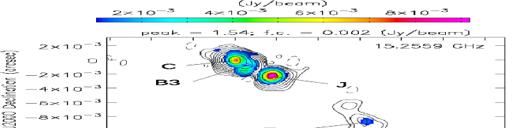
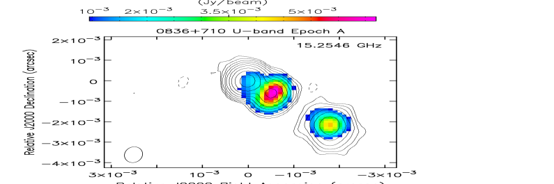
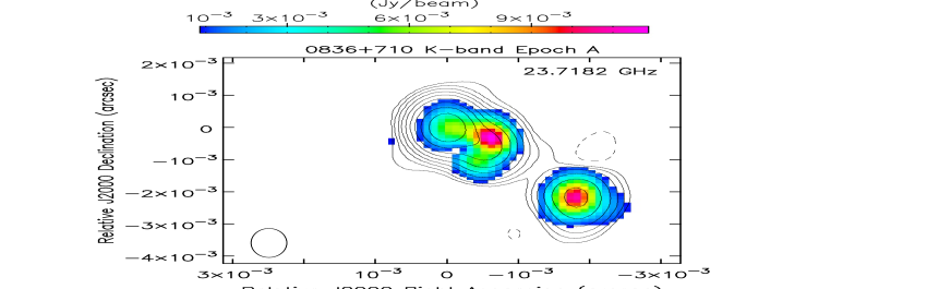
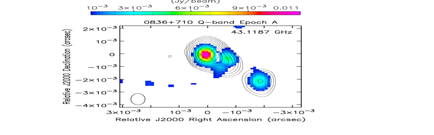
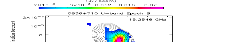
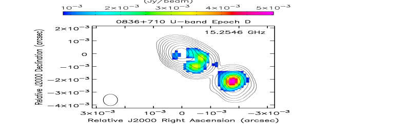
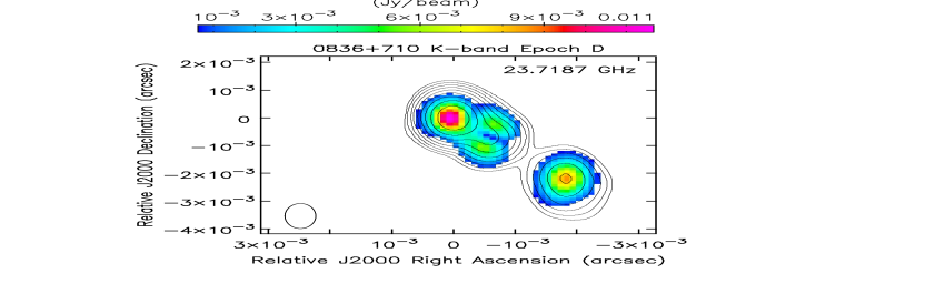
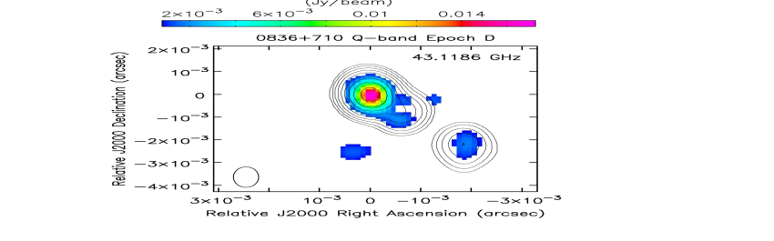
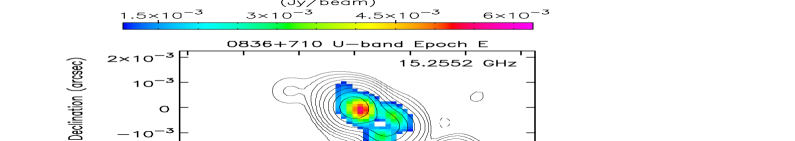
At parsec scale the radio source S5 0836$+$710 is characterized by a compact core and a jet that emerges from the core with a position angle (PA) of $-$130^∘ up to $\sim$10 mas and then changes to PA $-$155^∘ in agreement with previous studies (e.g. Krichbaum et al., 1990; Lobanov, 1998). The radio emission originates mainly in the radio core (component C in Fig. 5), which accounts for more than 65 per cent of the total flux density measured on our VLBA images. Two compact features are observed along the jet at $\sim$ 1 mas (component B3 in Fig. 5) and at $\sim$ 3 mas (component J in Fig. 5) from the core. Component B3 is resolved into two sub-components visible only in polarization intensity and labeled K1 and K2 in Fig. 5 (see Section 3.3). The low dynamic range of our observations prevents us from producing detailed images of the jet structure, and the region in which the jet changes the position angle is visible in some 15-GHz images only (Fig. 5). Multi-frequency VLBA flux densities are reported in Table 3. For a reliable comparison of flux density at different epochs for the main components we prefer to report the peak flux density measured on images obtained with the same beam. In fact our images are dynamic range limited and a variation of the total flux density may be not related to intrinsic variability of the component, but it may be due to the presence of low-surface brightness diffuse jet emission that is not detectable in all the observing epochs.
Fig. 6 shows the evolution of the peak flux density of component C, B3 and J. Between 2015 August and 2016 July the peak flux density at 43 GHz of component C shows a decreasing trend, whereas at 24 GHz an increase of the flux density is observed during the first two observing epochs, followed by a decreasing trend. At 15 GHz the variability is less evident with respect to the trend observed at higher frequencies. We observe a decrease of the flux density at each frequency for both components B3 and J, as expected in presence of adiabatic expansion.
To derive structural changes we complemented our observations with those from the VLBA-BU-BLAZAR program performed between 2014 September and 2018 May. To this aim we fitted the visibility data with circular Gaussian components at each epoch using the model-fit option in DIFMAP. This approach is used in order to derive small structure variation and provide an accurate fit of unresolved components close to the core component.

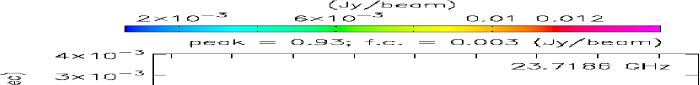
This analysis points out the presence of one (quasi-)stationary feature at about 0.03–0.1 mas from the core, labeled C1 in Fig. 7 with a position angle that ranges between $-$110^∘ and $-$140^∘, and two superluminal components, N and B3 with position angle of about $-$125^∘ and $-$140^∘, respectively. Component N is first detected by the visibility model-fit analysis at 43 GHz. Its presence on the image plane could be resolved at 43 GHz only after 2016 October. Fig. 8 shows the evolution of the flux density at 43 GHz of components C and C1 between 2014 September and 2018 May. The core component shows variability throughout the period, reaching a flux peak in 2015 April when the flux density doubled with respect to the value observed in 2015 February. The core peak flux density occurred close in time with the ejection of the new component N. In the same way, during the second half of 2015, when the $\gamma$-ray activity of the source was higher, the radio flux density of component C1 was higher than the values observed between 2014 September and 2015 February, reaching peak values in 2015 June and in September. After the high $\gamma$-ray activity period the flux density of C1 significantly decreased.

Figure 7: 43-GHz VLBA image from the observations performed on 2017 November 6 in the framework of the VLBA-BU-BLAZAR program. The image has been reconstructed with a beam of 0.1 $\times$ 0.1 mas². The peak flux density is 0.80 Jy/beam and the first contour is 1 per cent of the peak. Contour levels increase by a factor of 2. The restoring beam is plotted in the bottom left-hand corner. The grey-scale is shown by the wedge at the bottom of the figure and represents the total intensity flux density in Jy/beam.

Figure 8: Flux density at 43 GHz of the component C (top panel), and the component C1 (bottom panel) in the period 2014 September–2018 May. Vertical dashed lines mark the high-activity period in $\gamma$ rays (i.e. 2015 May–November).

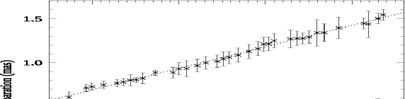
We derive the proper motion of these components by means of a linear fit. We find that component N is moving with an apparent velocity v_app = (14.8 $\pm$ 0.6)$c$ and the estimated epoch of passage through the VLBI core is 2015.28$\pm$0.07 (i.e. 2015 April), in good agreement with the increase of the flux density at 43 GHz (Fig. 3) and the beginning of the high-activity period observed in $\gamma$ rays. Component B3 is moving with an apparent velocity v_app = (21.0 $\pm$ 0.4)$c$, and corresponds to the component that emerged after the $\gamma$-ray flare in 2011 (Akyuz et al., 2013), discussed by Jorstad et al. (2017) and Jorstad et al. (2013). Results on the model-fit analysis of the visibility data are reported in Fig. 9 and in Appendix B. A stationary feature, labeled A1 in Fig. 7, at 0.1 mas on the opposite side of the core is present during the entire period monitored by our VLBA campaign. This feature was already reported by Jorstad et al. (2017).

Between 15 and 24 GHz the spectrum of the core is inverted after the $\gamma$-ray flare, with a spectral index $\alpha_{15}^{24}$ = 0.5 $\pm$ 0.3 (Fig. 10, right panel). Errors on the spectral index are computed in two steps. First, we determine the errors associated with the flux density scale uncertainty $\sigma_{c}$ such that:

$$\sigma_{c}=\sqrt{\left(\frac{\sigma_{\rm S1}}{S_{1}}\right)^{2}+\left(\frac{\sigma_{\rm S2}}{S_{2}}\right)^{2}}\frac{1}{{\rm ln(\nu_{2})-ln(\nu_{1})}}$$

where $S_{i}$ and $\sigma_{{\rm S}i}$ are the flux density and the flux density uncertainty, respectively, at the frequency $i$ (see Section 2). Then $\sigma_{c}$ is combined with the value from the spectral index error maps, $\sigma_{\alpha}$, obtained by error propagation theory. $\sigma_{c}$ is about 0.2, while $\sigma_{\alpha}$ is generally below 0.05 with the exception of the edges of the radio structures. The resulting error is $\sigma_{\rm tot}=\sqrt{\sigma_{c}^{2}+\sigma_{\alpha}^{2}}$, and is usually dominated by $\sigma_{c}$.
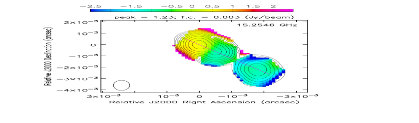
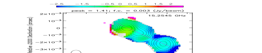
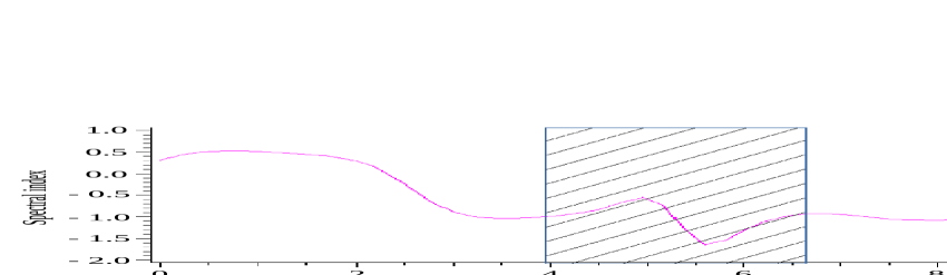
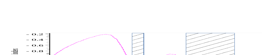
Fig. 10 shows how the ridge line spectral index values change across the source in 2015 August and 2016 July. In the former, the spectrum is inverted up to 2 mas from the core and then steepens smoothly, whereas in the latter the spectrum is steeper and a flattening is present at the position of B3 and corresponds to a peak in polarization (labelled K1 in Fig. 5). The gradients that are highlighted by a shaded area in Fig. 10 are likely due to (u,v)-coverage effects (see e.g. Hovatta et al., 2014). In these regions the values measured on the spectral index error images are $\sigma_{\alpha}>$ 0.3, i.e. more than an order of magnitude larger than in the other regions. In the last epochs the spectrum of the core flattens up to reaching $\alpha_{15}^{24}$ = $-$0.4 $\pm$ 0.3 in 2016 July (Fig. 10, bottom panel). Between 24 and 43 GHz the variation of the spectral shape is smoother and the spectral index $\alpha_{24}^{43}$ ranges between $-$0.1 $\pm$ 0.3 and $-$0.6 $\pm$ 0.3 (Fig. 6, bottom panel). Jet components have a steep spectrum ($-1.1<\alpha<-0.8$).

Figure 9: Separation of components from the core (dashed line) vs time. Labels refer to the source components found during the visibility model-fit analysis and reported in Fig. 7.

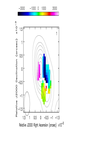
3.3 Polarization and Rotation Measure

Table 4: Polarized flux density measured on the full-resolution images. Images at the same frequency were reconstructed with the same restoring beam (see Section 2.3.2). Column 1: epoch of observations from Table 2. Columns 2, 3, and 4: core polarized flux density (mJy) at 15, 24 and 43 GHz, respectively. Columns 5, 6, and 7: component K2 polarized flux density (mJy) at 15, 24 and 43 GHz, respectively. Columns 8, 9, and 10: component K1 polarized flux density (mJy) at 15, 24 and 43 GHz, respectively. Columns 11, 12, and 13: component J polarized flux density (mJy) at 15, 24 and 43 GHz, respectively.

Epoch	C			K2			K1			J
	P15	P24	P43	P15	P24	P43	P15	P24	P43	P15	P24	P43
A	-	8.0$\pm$0.6	10.8$\pm$1.1	11.7$\pm$0.8	18.5$\pm$1.3	11.1$\pm$1.1	-	-	-	7.7$\pm$0.6	13.2$\pm$0.9	4.7$\pm$0.5
B	0.7$\pm$0.1	11.5$\pm$0.8	14.1$\pm$1.4	30.7$\pm$2.1	12.1$\pm$0.9	4.0$\pm$0.5	-	-	-	23.5$\pm$1.6	13.3$\pm$0.9	1.6$\pm$0.3
C	1.3$\pm$0.2	7.6$\pm$0.5	24.3$\pm$2.4	18.1$\pm$1.3	13.7$\pm$1.0	2.7$\pm$0.3	-	-	5.5$\pm$0.6	16.4$\pm$1.2	11.5$\pm$0.8	2.1$\pm$0.3
D	1.3$\pm$0.2	15.0$\pm$1.0	17.8$\pm$1.8	3.0$\pm$0.2	4.6$\pm$0.3	2.4$\pm$0.3	4.0$\pm$0.3	6.5$\pm$0.5	3.0$\pm$0.3	10.3$\pm$0.9	11.2$\pm$0.8	1.5$\pm$0.2
E	7.3$\pm$0.5	24.1$\pm$1.7	16.7$\pm$1.7	1.1$\pm$0.2	-	2.0$\pm$0.2	3.2$\pm$0.3	4.5$\pm$0.3	2.0$\pm$0.2	11.4$\pm$0.8	9.1$\pm$0.6	1.6$\pm$0.2
F	12.5$\pm$0.9	11.9$\pm$0.8	15.5$\pm$1.6	2.9$\pm$0.2	2.0$\pm$0.2	0.4$\pm$0.2	7.4$\pm$0.5	5.0$\pm$0.4	1.2$\pm$0.2	14.7$\pm$1.0	7.5$\pm$0.5	1.5$\pm$0.2

At 43 GHz and 24 GHz the core region is polarized during the entire monitoring campaign. No significant polarization ($<$1 mJy) is observed at 15 GHz in 2015 August, then the polarized flux density increases from 0.7 mJy in 2015 October up to $\sim$13 mJy in 2016 July. The polarized flux density reaches a maximum at 43 GHz in 2016 January followed with some time delay at 24 GHz and then at 15 GHz (see Table 4). This may be related to the change in opacity with time, suggested by the spectral index behaviour (see Fig. 6).
Significant polarization is observed for component J at each frequency during the whole monitoring period (Table 4). The polarization angle is stable at about 90^∘ at all frequencies, consistent with other VLBA observations at 15 GHz (Lister et al., 2018). As a consequence, no significant RM is observed in component J, and values are consistent with the errors.
Polarized emission from component B3 is detected during all epochs. At 24 GHz the polarized emission is resolved into two components, one to the north, K2 (with position angle $-$125^∘ with respect to the core component), and one to the south, K1 (with position angle $-$145^∘ with respect to the core component), of the peak of the B3 component as observed in total intensity images. The polarization morphology resembles a limb-brightened structure. At 15 GHz the two polarized components are resolved from 2016 March, whereas in the first three epochs they are blended together, in agreement with what is found by Lister et al. (2018). At 43 GHz polarized emission from component K1 is detected during all epochs with the exception of 2015 October, whereas significant polarized emission from component K2 is detected sporadically. Polarized flux density of the sub-components of S5 0836$+$710 are reported in Table 4, while the full set of polarization images are presented in Appendix C (Fig. 13).

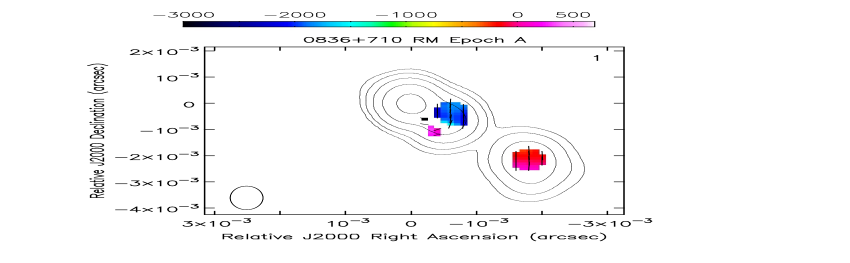
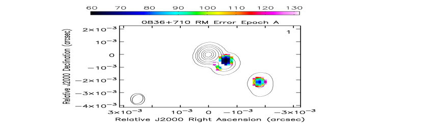
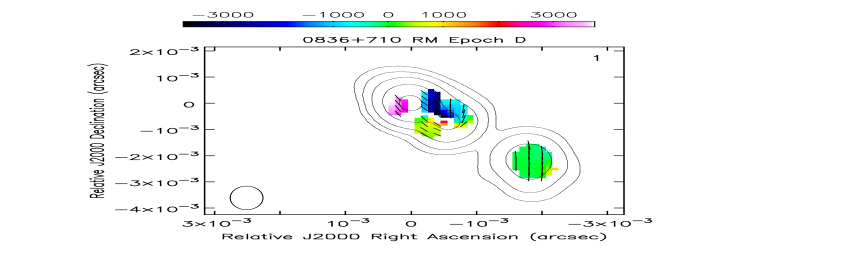
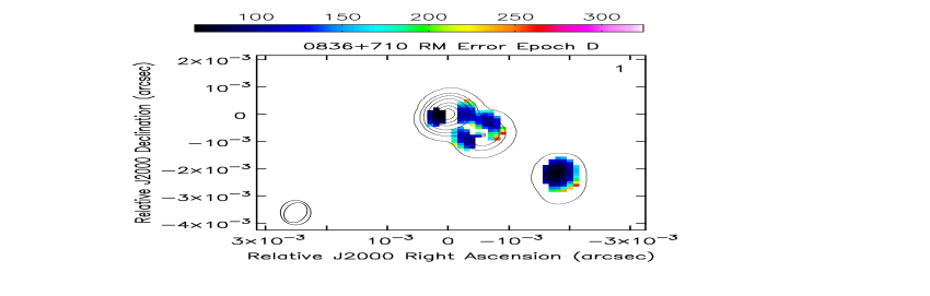
In the core component we observe very high values of RM, that may exceed $|$5000$|$ rad m^-2. The RM is highly variable with sign changes and its structure is patchy, indicating either opacity gradients and/or different components that evolve with time, expected in the case of a perturbed flow which is moving along the jet. In the last epoch, when the radiation is optically thin at all three frequencies, we observe an RM of $-$1400 $\pm$ 500 rad m^-2, and an RM-corrected magnetic field direction of 58 $\pm$ 5^∘, roughly parallel to the jet direction. RM-images and the associated error images at each observing epoch are presented in Fig. 11.

During the epochs in which component K2 has significant polarized emission at the three frequencies the RM is about $-$1950 $\pm$ 150 rad m^-2 in 2015 August, and $-$1200 $\pm$ 400 rad m^-2 in 2015 October and 2016 March. The RM-corrected magnetic field direction ranges between 160^∘ and 175^∘. Component K1 has RM values between 850 $\pm$ 120 and $-$180 $\pm$ 120 rad m^-2, with a tentative sign change observed in the last epoch, while the RM-corrected magnetic field direction ranges between 60^∘ and 75^∘, roughly parallel to the jet direction.
We perform the analysis of the jet transverse structure making use of the data taken in March 2016, i.e. when polarized emission from both K1 and K2 components is clearly visible at all frequencies. Fig. 12 indicates the RM image and the slice considered for the analysis. A transverse RM gradient is clearly visible with K1 component showing positive RM values, while K2 component has negative RM values (Fig. 12). The shaded area marks regions with low polarization levels consistent with noise, where no reliable RM could be estimated. Total intensity and polarization profiles on the same transverse slice show a ridge-brightened profile and a limb-brightened profile, respectively. The transverse spectral index profile between 15 and 24 GHz indicates a smooth flattening of the spectrum towards the ridge of the jet, with the spectral index values moving from about 1.0 at the borders to about 0.7 at the centre.

4 Discussion

4.1 Localization of the $\gamma$-ray emitting region and energetics

One of the main characteristics of blazars is the high variability in all bands, with a high fraction of energy in $\gamma$ rays. Information about the variability time-scale and the highest energy photons observed from a source may provide stringent constraints on the location of the $\gamma$-ray emitting region. Since most of the luminosity of blazars is often released at extreme energies, coverage of the $\gamma$-ray band is necessary to properly infer the energetic budget of these sources.
In FSRQ the $\gamma$-$\gamma$ collision between photons produced in the jet and broad line region (BLR) photons may produce a strong cut-off in the $\gamma$-ray spectrum above $\sim$ 20 GeV. In case of high-redshift blazars the $\gamma$-ray emission above a few GeV should be suppressed also by the pair production due to interaction of these $\gamma$-rays with the low-energy photons of the EBL. S5 0836$+$710 is not included in the Third Catalog of Hard Fermi-LAT sources (3FHL; Ajello et al., 2017), based on 7 years of LAT data analysed in the 10 GeV–2 TeV energy range, suggesting how difficult is to detect photons with energy higher than 10 GeV from S5 0836$+$710. The maximum photon energy observed from the source during 2014–2016 is 15.3 GeV, consistent with current EBL models for a source at redshift 2.2 (e.g., Finke et al., 2010; Dominguez et al., 2011). No evidence of cut-off in the $\gamma$-ray spectrum of the source due to $\gamma$-$\gamma$ interaction with BLR photons have been reported in Costamante et al. (2018). This suggests that the $\gamma$-ray emission from this source is due to inverse Compton (IC) scattering off infrared photons from the dusty torus and the spectrum above a few dozen GeV is significantly attenuated by the $\gamma$-$\gamma$ interaction with the EBL photons.

During the 2015 November flaring activity of S5 0836$+$710 significant $\gamma$-ray flux variation by a factor of 2 or more is clearly visible on 3-h time-scales. This short time variability observed in $\gamma$ rays constrains the size of the emitting region to $R<ct_{var}\delta/(1+z)$. Assuming a bulk Lorentz factor $\Gamma=$ 16 (Tagliaferri et al., 2015), we find that the size of the emitting region responsible for 3-h variability is R $\sim$ 2$\times$10¹⁵ cm. The inferred size is comparable to the gravitational radius (r${}_{\rm\,g}$/$c$ = G M /$c^{2}$) for a black hole with mass 5$\times$10⁹ M_⊙, as the one estimated for S5 0836$+$710 (Tagliaferri et al., 2015).

Although the high activity observed in the radio band starting at the beginning of 2015 does not seem associated with any significant increase of flux in the other bands, after the emergence of the new superluminal component we observe the beginning of high activity in $\gamma$ rays, X-rays, UV, and then in optical. The high activity in $\gamma$ rays reaches two peaks, in 2015 August and November, i.e., about 80 and 210 days after the ejection of the new component from the radio core. During this period the C1 component shows high variability, roughly doubling its flux density in one month, and its centroid moves from about 0.05 to 0.09 mas, which corresponds to a deprojected distance from the core of about 7–15 pc, assuming a viewing angle of 3.2 degrees (Pushkarev et al., 2009). These pieces of evidence suggest that a perturbed flow is moving along the jet and crosses the C1 component that may represent several standing shocks. Observations at higher resolution are necessary to confirm the presence of multiple shocks by resolving C1 into sub-components. In this scenario, the $\gamma$-ray activity should be produced at about 6 pc and 15 pc from the radio core, and the short-term $\gamma$-ray variability might be explained by the turbulent, extreme multi-zone model proposed by Marscher (2014), although magnetic reconnection cannot be excluded (e.g., Petropoulou et al., 2016). However, the sparse radio light curve does not allow us to claim a clear connection between the radio and optical-to-$\gamma$-ray variability. A similar conclusion was suggested for the flare observed in 2012 from the same source (Akyuz et al., 2013; Jorstad et al., 2013).

The interaction between a superluminal jet component and a standing shock as the origin of $\gamma$-ray flares has been proposed for several blazars, like the case of CTA 102 (Casadio et al., 2019), PKS 1510$-$089 (Marscher et al., 2010; Orienti et al., 2013), and BL Lacertae (Marscher et al., 2008). The lack of any evidence of $\gamma$-$\gamma$ absorption from the BLR during the high-activity period in S5 0836$+$710 supports the location of the $\gamma$-ray flaring region far away from the central region.

If we consider the $\gamma$-ray luminosity of S5 0836$+$710 at the daily peak ($\sim 2.6\times 10^{50}$ erg s^-1) as the total luminosity emitted during the major flare ($L_{\gamma,iso}$), after the beaming correction, we obtain the jet power spent to produce the observed radiation as $P_{\rm\,rad}$ $\simeq$ $L_{\gamma,iso}$ / 2$\Gamma^{2}$ = 5.0 $\times$ 10⁴⁷ erg s^-1 (assuming $\Gamma$ = 16). For a comparison, the radiative jet power is about 65 per cent of the Eddington luminosity (L${}_{\rm\,Edd}$ = 6.9 $\times$ 10⁴⁷ erg s^-1) and a factor of two higher than the accretion disc luminosity. Assuming that the radiative power is about 10 per cent of the total jet power (e.g., Celotti & Ghisellini, 2008), we have $P_{\rm jet,tot}$ = 5.0 $\times$ 10⁴⁸ erg s^-1. The total jet power can be compared to the accretion power, P${}_{\rm\,acc}$ = L${}_{\rm\,disc}$ / $\eta_{\rm disc}$ = 2.3$\times$10⁴⁸ erg s^-1 (assuming $\eta_{disc}$ = 0.1), indicating that the total jet power is larger than the accretion power in active states of S5 0836$+$710, as observed for other blazars (Ghisellini et al., 2014).

4.2 Jet structure

From the analysis of the multi-epoch polarimetry observations of S5 0836$+$710 we find that in the limb-brightened polarization structure that is observed at a projected distance of about 1 mas from the core, RM values vary between 1000 and -2000 rad m^-2. These values are much larger than those reported by Hovatta et al. (2012) for this source. However, in their work Hovatta et al. (2012) detected RM only from a component that is a few parsecs away from the core, and is likely consistent with component J, which also does not show any significant RM during our VLBA monitoring campaign. On the contrary, we observe some variability in the RM values observed in the limb-brightened polarization structure, as well as in the polarization intensity, suggesting that the Faraday screen and the emitting jet are closely connected. Furthermore, this structure shows a clear RM gradient transverse to the jet direction. In 2016 March the RM values vary from $\sim$800 to $\sim$ $-$1200 moving from the eastern to the western edge, with the exception of the central region where no significant polarization is detected. Gabuzda et al. (2017) found that a high fraction of the sources that were found to have a ‘spine-sheath’ polarization structure in Gabuzda et al. (2014) display transverse RM gradient with a high incidence of sign change. Detection of sign changes indicates a change in the direction of the line-of-sight magnetic field. Although we observe some RM variability in the limb-brightened polarization structure, the magnetic field direction in K1 is roughly parallel to the jet axis during the three epochs in which polarized emission from this component is clearly detected. These characteristics are consistent with a scenario in which Faraday rotation is produced by a sheath or boundary layer of thermal electrons with a toroidal magnetic field that surrounds the emitting jet (e.g. Broderick & McKinney, 2010). Gabuzda et al. (2014) observed for this source a transverse RM gradient with a sign change at 5 mas from the core. Interestingly, Asada et al. (2010) reported a similar result, but with the gradient moving in the opposite direction, which may be interpreted in terms of a change in domination between an inner and outer region of helical magnetic field as suggested for the jet in 1803+784 by Mahmud et al. (2009).
When polarization is detected in the core, the RM is highly variable and may exceed $|$5000$|$ rad m^-2. Such large values have been measured in the core region of other blazars (e.g. Jorstad et al., 2007; Hovatta et al., 2012) and may indicate that in this region the relation between the polarization vector and lambda square is not linear. As pointed out by the model-fit of visibility at 43 GHz, in the core region there are several components that are unresolved with the beam at 15 GHz, and blending of components with different opacity and polarization properties may cause spurious RM values (Hovatta et al., 2012). The variation of the spectral index of the core, from inverted soon after the $\gamma$-ray flare to slightly steep in the last observing epochs, suggests changes in opacity of the core region. A similar steepening of the core was observed in the VLBA monitoring of the high-z source TXS 0536+145 (Orienti et al., 2014). However, the lack of multi-frequency VLBA observations before the $\gamma$-ray flare precludes us to unambiguously connect the high opacity of the core region to the $\gamma$-ray flare.

Figure 10: Spectral index distribution between 15 and 24 GHz in 2015 August (top left panel) and in 2016 July (bottom left panel); spectral index values along the ridge line in 2015 August (top right panel) and in 2016 July (bottom right panel). The line indicates the slice used to derive the spectral profiles. Shaded areas represent regions of artificial gradients with high errors ($\sigma_{\alpha}>$ 0.3), likely caused by poor (u,v)-coverage.

Figure 11: Rotation measure images (colour-scale) for S5 0836$+$710 overlaid with total intensity contours (left column), and the associated rotation measure error images (colour-scale; right column). Vectors represent the RM-corrected magnetic field (B) vectors.

Figure 11: continued

Figure 12: Rotation measure map of S5 0836$+$710 in 2016 March (top panel). The line represents the transverse slice used for the analysis. Middle left panel: total intensity profile; middle right panel: polarization profile; bottom left panel: RM profile; bottom right panel: spectral index profile between 15 and 24 GHz.

5 Summary

In this paper we reported on results of a broad-band monitoring campaign, from radio to $\gamma$ rays, of the high redshift FSRQ S5 0836$+$710 following a period of high activity detected by Fermi-LAT. During the $\gamma$-ray flares the apparent isotropic $\gamma$-ray luminosity of the source exceeds 10⁵⁰ erg s^-1, similar to other high-redshift objects detected in flares by Fermi-LAT. In particular, on 2015 November 9 (MJD 57335) the source reached on 3-hour time-scale the highest $\gamma$-ray luminosity observed by a blazar ($\sim$3.7 $\times$ 10⁵⁰ erg s^-1). The flux doubling time of 3 hours at the peak of the $\gamma$-ray activity indicates that the size of the emitting region is comparable to the gravitational radius for this source.

The high $\gamma$-ray activity observed in 2015 might be related to the new superluminal component that emerged from the core at the peak of the radio activity, with the short variability explained by a strong turbulence in the jet plasma or magnetic reconnection. However, the available data cannot allow us to infer a clear connection between the radio and the $\gamma$-ray activity.

The smaller variability observed in X-rays with respect to $\gamma$ rays may indicate that the X-ray emission is produced by the low-energy tail of the same electron distribution that produces the $\gamma$-ray emission through IC. The optical-UV part of the spectrum of the source is dominated by the accretion disc emission also during high activity states. The small variability observed in optical and UV bands during our monitoring campaign, suggests that the optical-UV part of the spectrum has a large contribution from the accretion disc.

The analysis of multi-epoch full polarization radio observations suggests a change in the opacity in the core component with time with a steepening of the spectral index during the latest observing epochs. Although in total intensity the jet has a ridge-brightened structure, the polarized emission has a clear limb-brightened structure in which a RM gradient is observed transverse to the jet direction. Furthermore, some RM variability is observed in the core and jet structures with the exception of a knot in the jet with stable RM. The polarization properties are consistent with a helical field in a two-fluid jet model, consisting of an inner, emitting jet and a sheath containing non-relativistic electrons. In addition, we observe a region with highly ordered magnetic field in which strong shocks are likely taking place. However the low dynamic range of these observations could not allow us to study in detail the polarization structure at large distances and deeper observations are needed for a better characterization of the magnetic field along the jet.

Appendix A Swift data results

Table 5: Log and fitting results of Swift-XRT observations of S5 0836$+$710 using a PL model with $N_{\rm H}$ fixed to Galactic absorption.

MJD	Date (UT)	Net exposure time	Photon index	Flux 0.3–10 keVa	$\chi^{2}$ / d.o.f.
		(sec)	($\Gamma_{\rm\,X}$)	($\times$10-11 erg cm-2 s-1)
56675	2014-01-18	4735	1.32 $\pm$ 0.05	3.86 $\pm$ 0.19	67/80
56778	2014-05-01	649	1.23 $\pm$ 0.16	2.86 $\pm$ 0.38	9/12
56783	2014-05-06	719	1.14 $\pm$ 0.15	2.73 $\pm$ 0.39	13/12
56804	2014-05-27	1076	1.29 $\pm$ 0.12	3.28 $\pm$ 0.36	17/14
56832	2014-06-24	415	1.08 $\pm$ 0.21	5.84 $\pm$ 1.09	6/7
56836	2014-06-28	824	1.41 $\pm$ 0.09	4.57 $\pm$ 0.37	33/29
56947	2014-10-17	9709	1.19 $\pm$ 0.03	2.93 $\pm$ 0.10	161/170
56987	2014-11-26	4700	1.17 $\pm$ 0.05	3.01 $\pm$ 0.14	68/98
57008	2014-12-17	5017	1.23 $\pm$ 0.05	2.51 $\pm$ 0.12	90/86
57039	2015-01-17	4792	1.31 $\pm$ 0.05	2.37 $\pm$ 0.12	91/80
57070	2015-02-17	4755	1.21 $\pm$ 0.07	2.15 $\pm$ 0.13	58/58
57098	2015-03-17	1104	1.29 $\pm$ 0.15	1.90 $\pm$ 0.23	10/14
57101	2015-03-20	3718	1.25 $\pm$ 0.08	1.85 $\pm$ 0.14	33/42
57128	2015-04-16	4550	1.33 $\pm$ 0.06	1.51 $\pm$ 0.09	68/55
57159	2015-05-17	3174	1.33 $\pm$ 0.08	1.79 $\pm$ 0.13	50/42
57162	2015-05-20	1608	1.40 $\pm$ 0.11	1.82 $\pm$ 0.17	26/24
57193	2015-06-20	2023	1.46 $\pm$ 0.07	2.85 $\pm$ 0.18	45/47
57196	2015-06-23	2108	1.39 $\pm$ 0.07	2.90 $\pm$ 0.18	60/52
57220	2015-07-17	4915	1.16 $\pm$ 0.04	3.35 $\pm$ 0.14	119/115
57243	2015-08-09	954	1.25 $\pm$ 0.13	2.89 $\pm$ 0.32	21/19
57245	2015-08-11	2677	1.28 $\pm$ 0.08	2.38 $\pm$ 0.16	44/44
57247	2015-08-13	2103	1.38 $\pm$ 0.17	2.35 $\pm$ 0.40	30/39
57249	2015-08-15	2957	1.28 $\pm$ 0.06	2.58 $\pm$ 0.15	65/58
57251	2015-08-17	1915	1.23 $\pm$ 0.09	2.42 $\pm$ 0.20	46/37
57254	2015-08-20	3276	1.27 $\pm$ 0.08	2.10 $\pm$ 0.15	49/49
57282	2015-09-17	3971	1.31 $\pm$ 0.06	2.54 $\pm$ 0.14	77/62
57325	2015-10-30	2924	1.19 $\pm$ 0.06	5.14 $\pm$ 0.30	65/62
57327	2015-11-01	1915	1.21 $\pm$ 0.08	4.34 $\pm$ 0.34	33/37
57329	2015-11-03	5042	1.18 $\pm$ 0.05	4.51 $\pm$ 0.21	106/96
57331	2015-11-05	2320	1.10 $\pm$ 0.08	4.48 $\pm$ 0.36	29/39
57333	2015-11-07	2929	1.11 $\pm$ 0.05	4.36 $\pm$ 0.22	73/85
57336	2015-11-10	1968	1.16 $\pm$ 0.08	5.49 $\pm$ 0.41	39/44
57359	2015-12-03	4827	1.27 $\pm$ 0.05	2.71 $\pm$ 0.12	99/99
57401	2016-01-14	4665	1.26 $\pm$ 0.05	2.74 $\pm$ 0.13	96/91
57421	2016-02-03	2632	1.30 $\pm$ 0.07	2.87 $\pm$ 0.18	47/52
57425	2016-02-07	2602	1.36 $\pm$ 0.07	2.65 $\pm$ 0.16	46/55
57450	2016-03-03	3207	1.28 $\pm$ 0.07	2.74 $\pm$ 0.17	58/57
57464	2016-03-17	3359	1.22 $\pm$ 0.07	3.32 $\pm$ 0.22	50/48
57469	2016-03-22	1408	1.31 $\pm$ 0.13	3.32 $\pm$ 0.36	17/19
57481	2016-04-03	4420	1.20 $\pm$ 0.06	2.64 $\pm$ 0.14	80/80
57511	2016-05-03	4445	1.19 $\pm$ 0.05	4.07 $\pm$ 0.18	123/107
57540	2016-06-01	3526	1.11 $\pm$ 0.07	3.07 $\pm$ 0.22	80/68
57572	2016-07-03	4917	1.17 $\pm$ 0.05	3.06 $\pm$ 0.14	112/103

^aUnabsorbed flux

Table 6: Observed magnitudes obtained by Swift-UVOT for S5 0836$+$710.

MJD	Date (UT)	$v$	$b$	$u$	$w1$	$m2$	$w2$
56675	2014-01-18	16.91 $\pm$ 0.10	17.11 $\pm$ 0.07	16.23 $\pm$ 0.07	16.86 $\pm$ 0.10	17.54 $\pm$ 0.12	17.90 $\pm$ 0.11
56778	2014-05-01	16.55 $\pm$ 0.31	17.06 $\pm$ 0.08	16.38 $\pm$ 0.08	17.06 $\pm$ 0.11	-	18.08 $\pm$ 0.13
56783	2014-05-06	16.87 $\pm$ 0.14	17.26 $\pm$ 0.10	17.26 $\pm$ 0.09	17.02 $\pm$ 0.13	17.68 $\pm$ 0.16	17.86 $\pm$ 0.14
56804	2014-05-27	17.04 $\pm$ 0.13	17.03 $\pm$ 0.09	16.18 $\pm$ 0.08	17.03 $\pm$ 0.11	17.44 $\pm$ 0.13	17.70 $\pm$ 0.11
56832	2014-06-24	16.81 $\pm$ 0.19	17.10 $\pm$ 0.14	16.10 $\pm$ 0.11	16.91 $\pm$ 0.15	17.74 $\pm$ 0.23	17.78 $\pm$ 0.16
56836	2014-06-28	16.94 $\pm$ 0.20	17.20 $\pm$ 0.14	16.23 $\pm$ 0.11	16.79 $\pm$ 0.14	17.47 $\pm$ 0.22	17.84 $\pm$ 0.17
56947	2014-10-17	16.93 $\pm$ 0.17	17.13 $\pm$ 0.10	16.37 $\pm$ 0.10	16.99 $\pm$ 0.13	17.56 $\pm$ 0.15	17.64 $\pm$ 0.13
56987	2014-11-26	16.94 $\pm$ 0.16	17.24 $\pm$ 0.12	16.24 $\pm$ 0.09	17.16 $\pm$ 0.14	17.50 $\pm$ 0.15	17.85 $\pm$ 0.14
57008	2014-12-17	17.06 $\pm$ 0.10	17.15 $\pm$ 0.07	16.30 $\pm$ 0.07	17.13 $\pm$ 0.10	17.63 $\pm$ 0.12	17.93 $\pm$ 0.10
57039	2015-01-17	17.07 $\pm$ 0.11	17.16 $\pm$ 0.08	16.34 $\pm$ 0.07	17.07 $\pm$ 0.11	17.68 $\pm$ 0.14	18.05 $\pm$ 0.12
57070	2015-02-17	17.09 $\pm$ 0.10	17.13 $\pm$ 0.07	16.32 $\pm$ 0.07	17.08 $\pm$ 0.10	17.83 $\pm$ 0.13	17.98 $\pm$ 0.11
57098	2015-03-17	17.12 $\pm$ 0.12	17.11 $\pm$ 0.08	16.32 $\pm$ 0.08	17.00 $\pm$ 0.11	17.43 $\pm$ 0.13	17.93 $\pm$ 0.12
57101	2015-03-20	16.92 $\pm$ 0.10	17.12 $\pm$ 0.07	16.35 $\pm$ 0.07	17.01 $\pm$ 0.10	17.58 $\pm$ 0.12	18.07 $\pm$ 0.11
57128	2015-04-16	17.01 $\pm$ 0.14	17.16 $\pm$ 0.10	16.26 $\pm$ 0.09	16.97 $\pm$ 0.11	17.37 $\pm$ 0.12	18.09 $\pm$ 0.14
57159	2015-05-17	17.15 $\pm$ 0.13	17.11 $\pm$ 0.08	16.28 $\pm$ 0.08	16.99 $\pm$ 0.11	17.40 $\pm$ 0.13	17.75 $\pm$ 0.11
57162	2015-05-20	16.96 $\pm$ 0.10	17.23 $\pm$ 0.08	16.23 $\pm$ 0.07	16.97 $\pm$ 0.10	17.38 $\pm$ 0.11	17.84 $\pm$ 0.11
57193	2015-06-20	16.98 $\pm$ 0.15	17.07 $\pm$ 0.10	16.08 $\pm$ 0.08	16.91 $\pm$ 0.13	17.72 $\pm$ 0.21	17.80 $\pm$ 0.14
57196	2015-06-23	16.90 $\pm$ 0.16	17.07 $\pm$ 0.09	16.23 $\pm$ 0.08	17.07 $\pm$ 0.12	17.51 $\pm$ 0.19	18.12 $\pm$ 0.14
57220	2015-07-17	17.05 $\pm$ 0.16	17.22 $\pm$ 0.11	16.36 $\pm$ 0.09	16.98 $\pm$ 0.12	17.60 $\pm$ 0.15	17.90 $\pm$ 0.13
57243	2015-08-09	17.05 $\pm$ 0.17	17.10 $\pm$ 0.11	16.37 $\pm$ 0.10	17.17 $\pm$ 0.16	17.38 $\pm$ 0.15	17.89 $\pm$ 0.14
57245	2015-08-11	17.01 $\pm$ 0.13	17.05 $\pm$ 0.10	16.26 $\pm$ 0.09	17.09 $\pm$ 0.13	17.66 $\pm$ 0.14	17.92 $\pm$ 0.25
57247	2015-08-13	16.95 $\pm$ 0.15	17.22 $\pm$ 0.11	16.39 $\pm$ 0.10	17.03 $\pm$ 0.13	17.59 $\pm$ 0.16	17.94 $\pm$ 0.15
57249	2015-08-15	17.01 $\pm$ 0.12	17.25 $\pm$ 0.10	16.32 $\pm$ 0.08	17.05 $\pm$ 0.10	17.64 $\pm$ 0.12	17.95 $\pm$ 0.11
57251	2015-08-17	-	17.21 $\pm$ 0.08	16.38 $\pm$ 0.08	17.23 $\pm$ 0.11	-	17.80 $\pm$ 0.23
57254	2015-08-20	16.89 $\pm$ 0.18	17.33 $\pm$ 0.14	16.47 $\pm$ 0.11	17.18 $\pm$ 0.16	17.60 $\pm$ 0.17	17.81 $\pm$ 0.16
57282	2015-09-17	17.18 $\pm$ 0.22	16.95 $\pm$ 0.11	16.28 $\pm$ 0.11	17.25 $\pm$ 0.19	17.55 $\pm$ 0.27	17.87 $\pm$ 0.18
57325	2015-10-30	16.68 $\pm$ 0.10	16.83 $\pm$ 0.08	16.11 $\pm$ 0.07	16.73 $\pm$ 0.11	17.39 $\pm$ 0.08	17.64 $\pm$ 0.12
57327	2015-11-01	16.98 $\pm$ 0.12	17.14 $\pm$ 0.09	16.21 $\pm$ 0.08	16.85 $\pm$ 0.11	17.33 $\pm$ 0.13	17.81 $\pm$ 0.12
57329	2015-11-03	17.10 $\pm$ 0.18	17.05 $\pm$ 0.09	16.38 $\pm$ 0.09	16.97 $\pm$ 0.13	17.26 $\pm$ 0.17	17.77 $\pm$ 0.14
57331	2015-11-05	16.87 $\pm$ 0.17	17.13 $\pm$ 0.11	16.33 $\pm$ 0.10	16.97 $\pm$ 0.15	17.89 $\pm$ 0.20	17.59 $\pm$ 0.15
57333	2015-11-07	16.99 $\pm$ 0.13	17.06 $\pm$ 0.09	16.24 $\pm$ 0.08	16.99 $\pm$ 0.12	17.38 $\pm$ 0.13	17.84 $\pm$ 0.13
57336	2015-11-10	16.89 $\pm$ 0.11	17.12 $\pm$ 0.08	16.25 $\pm$ 0.08	16.86 $\pm$ 0.11	17.33 $\pm$ 0.10	17.63 $\pm$ 0.11
57359	2015-12-03	16.82 $\pm$ 0.10	17.10 $\pm$ 0.07	16.18 $\pm$ 0.07	16.85 $\pm$ 0.09	17.37 $\pm$ 0.11	17.85 $\pm$ 0.11
57401	2016-01-14	16.75 $\pm$ 0.10	16.98 $\pm$ 0.08	16.17 $\pm$ 0.07	16.78 $\pm$ 0.10	17.38 $\pm$ 0.13	17.58 $\pm$ 0.14
57421	2016-02-03	16.90 $\pm$ 0.11	16.94 $\pm$ 0.08	16.17 $\pm$ 0.07	16.89 $\pm$ 0.11	17.46 $\pm$ 0.14	17.75 $\pm$ 0.12
57425	2016-02-07	16.73 $\pm$ 0.11	16.99 $\pm$ 0.08	16.07 $\pm$ 0.07	16.79 $\pm$ 0.11	17.54 $\pm$ 0.14	17.58 $\pm$ 0.11
57450	2016-03-03	16.72 $\pm$ 0.14	16.90 $\pm$ 0.10	16.21 $\pm$ 0.10	16.91 $\pm$ 0.14	17.36 $\pm$ 0.17	17.67 $\pm$ 0.15
57464	2016-03-17	16.86 $\pm$ 0.17	16.88 $\pm$ 0.11	16.06 $\pm$ 0.10	16.96 $\pm$ 0.16	17.25 $\pm$ 0.15	17.57 $\pm$ 0.16
57469	2016-03-22	16.83 $\pm$ 0.12	17.06 $\pm$ 0.09	16.10 $\pm$ 0.08	16.85 $\pm$ 0.12	17.43 $\pm$ 0.14	17.76 $\pm$ 0.14
57481	2016-04-03	16.68 $\pm$ 0.13	17.00 $\pm$ 0.10	16.17 $\pm$ 0.09	16.98 $\pm$ 0.13	17.53 $\pm$ 0.16	17.56 $\pm$ 0.13
57511	2016-05-03	16.80 $\pm$ 0.09	17.07 $\pm$ 0.07	16.17 $\pm$ 0.07	16.82 $\pm$ 0.09	17.35 $\pm$ 0.12	17.63 $\pm$ 0.10
57540	2016-06-01	16.74 $\pm$ 0.15	16.98 $\pm$ 0.11	16.12 $\pm$ 0.09	17.03 $\pm$ 0.19	17.24 $\pm$ 0.13	17.71 $\pm$ 0.14
57572	2016-07-03	16.90 $\pm$ 0.14	17.10 $\pm$ 0.10	16.15 $\pm$ 0.08	16.77 $\pm$ 0.10	17.36 $\pm$ 0.12	17.57 $\pm$ 0.11

Appendix B Model-fit analysis

To derive structural changes we complemented our observations with those from the VLBA Boston University blazar (VLBA-BU-BLAZAR) program performed between 2015 May and 2018 May. To this aim we fitted the visibility data with circular Gaussian components at each epoch using the model-fitting option in DIFMAP. This approach is used in order to derive small structure variation and provide an accurate fit of unresolved components close to the core components. Direct comparison of models obtained independently at each epoch is not the best approach to detect small changes (Conway et al., 1992). For this reason, we produced a zero-order model consisting of four circular Gaussian components, which was used as the initial model in model-fitting the visibility data of each observing epoch. The convergence of the fit is reached when both the core and A1 components are considered point-like sources. After 2016 March an additional circular component was included in the model. Results are reported in Table 7.
Errors on the component position are $\Delta r=a/(S_{\rm p}/{\rm rms})$, where $a$ is the component deconvolved major-axis, $S_{\rm p}$ is the component peak flux density and the rms is the 1$\sigma$ noise level measured on the image plane. In case the errors are unreliably small, we assume a more conservative value that corresponds to 10 per cent of the beam (e.g. Orienti et al., 2011).

Table 7: Results of the visibility model-fit analysis at 43 GHz. Column 1: observing epoch; column 2: source component as from Fig. 7; column 3: flux density at 43 GHz (in mJy); column 4: component angular size (in milliarcsecond); Column 5: distance from the core component (in milliarcsecond); column 6: position angle with respect to the core component (in degree).

Epoch	Comp.	$S_{\rm 43GHz}$	$a$	$r$	$\Theta$
23/09/2014	C	808	-	-	-
	C1	199	0.14	0.024	$-$133
	B3	440	0.40	0.610	$-$136
	A1	523	-	0.100	54
05/12/2014	C	515	-	-	-
	C1	543	0.05	0.082	$-$106
	B3	328	0.41	0.715	$-$136
	A1	107	-	0.087	24
29/12/2014	C	814	-	-	-
	C1	428	0.01	0.080	$-$102
	B3	330	0.41	0.730	$-$136
	A1	109	-	0.065	9
15/02/2015	C	530	-	-	-
	C1	290	0.07	0.098	$-$133
	B3	312	0.40	0.750	$-$136
	A1	856	-	0.040	165
12/04/2015	C	1185	-	-	-
	C1	689	0.03	0.070	$-$97
	B3	315	0.41	0.770	$-$136
	A1	220	-	0.050	19
11/05/2015	C	948	-	-	-
	C1	532	0.094	0.055	$-$101
	B3	211	0.240	0.781	$-$137
	A1	271	-	0.075	57
09/06/2015	C	778	-	-	-
	C1	1080	0.094	0.057	$-$104
	B3	305	0.360	0.802	$-$136
	A1	141	-	0.101	36
02/07/2015	C	684	-	-	-
	C1	658	0.094	0.054	$-$122
	B3	193	0.240	0.807	$-$137
	A1	286	-	0.074	57
15/08/2015	C	655	-	-	-
	C1	481	0.094	0.070	$-$111
	B3	172	0.250	0.825	$-$138
	A1	306	-	0.079	52
22/09/2015	C	873	-	-	-
	C1	846	0.094	0.092	$-$117
	B3	190	0.250	0.890	$-$138
	A1	95	-	0.111	37
05/12/2015	C	887	-	-	-
	C1	102	0.094	0.094	$-$120
	B3	148	0.290	0.888	$-$138
	A1	240	-	0.095	45
01/01/2016	C	695	-	-	-
	C1	465	0.093	0.097	$-$120
	B3	133	0.280	0.932	$-$139
	A1	110	-	0.113	48
31/01/2016	C	740	-	-	-
	C1	411	0.093	0.110	$-$117
	B3	180	0.370	0.935	$-$138
	A1	180	-	0.110	38
18/03/2016	C	420	-	-	-
	C1	228	0.093	0.023	177
	N	308	0.130	0.134	$-$123
	B3	133	0.310	0.967	$-$139
	A1	221	-	0.106	37
22/04/2016	C	502	-	-	-
	C1	303	0.093	0.039	$-$155
	N	232	0.130	0.168	$-$124
	B3	123	0.320	1.000	$-$140
	A1	195	-	0.102	41

Table 7: Continued.

Epoch	Comp.	$S_{\rm 43GHz}$	$a$	$r$	$Theta$
10/06/2016	C	557	-	-	-
	C1	216	0.094	0.090	$-$131
	N	122	0.130	0.233	$-$122
	B3	105	0.330	1.017	$-$140
	A1	171	-	0.119	38
04/07/2016	C	419	-	-	-
	C1	249	0.091	0.070	$-$134
	N	148	0.130	0.220	$-$123
	B3	105	0.340	1.045	$-$140
	A1	178	-	0.118	41
16/08/2016	C	549	-	-	-
	C1	266	0.110	0.086	$-$121
	N	157	0.120	0.240	$-$123
	B3	150	0.340	1.060	$-$140
	A1	258	-	0.127	36
05/09/2016	C	446	-	-	-
	C1	296	0.092	0.076	$-$137
	N	193	0.130	0.246	$-$124
	B3	127	0.335	1.087	$-$141
	A1	235	-	0.112	41
23/10/2016	C	214	-	-	-
	C1	222	0.090	0.101	$-$135
	N	156	0.140	0.288	$-$126
	B3	94	0.360	1.128	$-$141
28/11/2016	C	148	-	-	-
	C1	159	0.080	0.086	$-$135
	N	138	0.160	0.280	$-$126
	B3	81	0.360	1.159	$-$142
	A1	157	-	0.112	39
23/12/2016	C	102	-	-	-
	C1	340	0.090	0.098	$-$153
	N	254	0.200	0.311	$-$131
	B3	120	0.350	1.210	$-$142
	A1	255	-	0.060	61
14/01/2017	C	222	-	-	-
	C1	201	0.090	0.112	$-$139
	N	193	0.170	0.328	$-$131
	B3	105	0.370	1.214	$-$142
	A1	228	-	0.070	40
04/02/2017	C	273	-	-	-
	C1	202	0.070	0.115	$-$142
	N	180	0.200	0.353	$-$128
	B3	90	0.350	1.249	$-$142
	A1	191	-	0.047	36
16/04/2017	C	322	-	-	-
	C1	182	0.080	0.064	$-$130
	N	156	0.240	0.364	$-$128
	B3	66	0.360	1.270	$-$141
	A1	122	-	0.061	29
13/05/2017	C	536	-	-	-
	C1	312	0.060	0.050	$-$124
	N	216	0.240	0.377	$-$128
	B3	95	0.360	1.276	$-$141
	A1	280	-	0.070	33
08/06/2017	C	847	-	-	-
	C1	164	0.050	0.069	$-$135
	N	226	0.240	0.365	$-$127
	B3	101	0.360	1.275	$-$142
	A1	194	-	0.088	44
03/07/2017	C	713	-	-	-
	C1	278	0.090	0.047	$-$138
	N	189	0.180	0.376	$-$128
	B3	96	0.410	1.291	$-$141
	A1	176	-	0.098	46

Table 7: Continued.

Epoch	Comp.	$S_{\rm 43GHz}$	$a$	$r$	$Theta$
06/08/2017	C	497	-	-	-
	C1	200	0.060	0.043	$-$135
	N	153	0.200	0.368	$-$127
	B3	56	0.300	1.339	$-$141
	A1	178	-	0.104	48
04/09/2017	C	338	-	-	-
	C1	404	0.070	0.025	$-$121
	N	153	0.190	0.389	$-$127
	B3	75	0.420	1.339	$-$142
	A1	206	-	0.111	43
06/11/2017	C	407	-	-	-
	C1	440	0.080	0.030	$-$128
	N	145	0.220	0.417	$-$127
	B3	59	0.080	1.395	$-$141
	A1	220	-	0.103	48
17/02/2018	C	171	-	-	-
	C1	485	0.100	0.017	179
	N	117	0.310	0.452	$-$129
	B3	49	0.280	1.443	$-$142
	A1	124	-	0.137	50
10/03/2018	C	507	-	-	-
	C1	232	0.090	0.064	$-$129
	N	109	0.270	0.497	$-$127
	B3	62	0.370	1.437	$-$141
	A1	208	-	0.123	38
19/04/2018	C	499	-	-	-
	C1	394	0.080	0.073	$-$144
	N	110	0.310	0.533	$-$128
	B3	48	0.250	1.500	$-$140
	A1	287	-	0.110	41
11/05/2018	C	390	-	-	-
	C1	451	0.080	0.070	$-$137
	N	119	0.310	0.537	$-$128
	B3	50	0.310	0.537	$-$140
	A1	322	-	0.109	37

Appendix C Multi-epoch polarization images

Figure 13: VLBA images of the source S5 0836$+$710. The colour-scale represents the polarization intensity, while contours are the total intensity. The first contour is about $\sim$3 mJy/beam, which corresponds to three times the off-source noise level. Contour levels increase by a factor of 2. All the images have been reconstructed with the same beam, which is plotted on the bottom left-hand corner. On each image we report the observing frequency (and band), and the observing epoch.

Figure 13: continued.

References

- Abdo et al. (2015) Abdo, A.A., et al. 2015, ApJ, 799, 143
- Abdollahi et al. (2018) Abdollahi, S., et al. 2019, Science, 362, 1031
- Acero et al. (2016) Acero, F., et al. 2016, ApJS, 223, 2
- Ackermann et al. (2015) Ackermann, M., et al. 2015, ApJ, 810, 14
- Akyuz et al. (2013) Akyuz, A., et al. 2013, A&A, 556,71
- Asada et al. (2010) Asada, K., Nakamura, M., Inoue, M., Kameno, S., Nagai, H. 2010, ApJ, 720, 41
- Atwood et al. (2009) Atwood, W. B., et al. 2009, ApJ, 697, 1071
- Atwood et al. (2013) Atwood, W. B., et al. 2013, 2012 Fermi Symposium proceedings - eConf C121028 (arXiv:1303.3514)
- Ajello et al. (2017) Ajello, M., et al. 2017, ApJS, 232, 18
- Barthelmy et al. (2005) Barthelmy, S. D., et al. 2005, Space Sci. Rev., 120, 143
- Beckmann et al. (2009) Beckmann, V., et al. 2009, A&A 505, 417
- Breeveld et al. (2010) Breeveld, A. A., et al. 2010, MNRAS, 406, 1687
- Broderick & McKinney (2010) Broderick, A.E., McKinney, J.C. 2010, ApJ, 725, 750
- Burrows et al. (2005) Burrows, D. N., et al. 2005, Space Sci. Rev., 120, 165
- Cardelli et al. (1989) Cardelli, J. A., Clayton, G. C., Mathis, J. S. 1989, ApJ, 345, 245
- Casadio et al. (2019) Casadio, C., et al. 2019, A&A, 622, 158
- Celotti & Ghisellini (2008) Celotti, A., Ghisellini, G. 2008, MNRAS, 385, 1283
- Ciprini (2015) Ciprini, S. 2015, The Astronomer’s Telegram, 7870
- Collmar et al. (2006) Collmar, W. 2006, ASPC, 350, 120
- Conway et al. (1992) Conway, J.E., Pearson, T.J., Readhead, A.C.S., Unwin, S.C., Xu, W., Mutel, R.L. 1992, ApJ, 396, 62
- Costamante et al. (2018) Costamante, L., Cutini, S., Tosti, G., Antolini, E., Tramacere, A. 2018, MNRAS, 477, 4749
- D’Ammando et al. (2011) D’Ammando, F., et al. 2011, A&A, 529A, 145
- D’Ammando & Orienti (2016) D’Ammando, F., & Orienti, M. 2016, MNRAS, 455, 1881
- Dominguez et al. (2011) Dominguez, A., et al. 2011, MNRAS, 410, 2556
- Dominguez & Ajello (2015) Dominguez, A., & Ajello, M. 2015, ApJ, 813L, 34
- Finke et al. (2010) Finke J. D., Razzaque S., Dermer C. D., 2010, ApJ, 712, 238
- Gabuzda et al. (2014) Gabuzda, D.C., Reichstein, A.R., O’Neill, E.L. 2014, MNRAS, 444, 172
- Gabuzda et al. (2017) Gabuzda, D.C., Roche, N., Kirwan, A., Knuettel, S., Nagle, M., Houston, C. 2017, MNRAS, 472, 1792
- Gehrels et al. (2004) Gehrels, N., et al. 2004, ApJ, 611, 1005
- Ghisellini et al. (2014) Ghisellini, G., et al. 2014, Nature, 515, 376
- Gomez et al. (2011) Gómez, J.L., Roca-Sogorb, M., Agudo, I., Marscher, A.P., Jorstad, S.G. 2011, ApJ, 733, 11
- Hovatta et al. (2012) Hovatta, T., Lister, M.L., Aller, M.F., Aller, H.D., Homan, D.C., Kovalev, Y.Y., Pushkarev, A.B., Savolainen, T. 2012, AJ, 144, 105
- Hovatta et al. (2014) Hovatta, T., et al. 2014, ApJ, 147, 143
- Jorstad et al. (2007) Jorstad, S.G., et al. 2007, AJ, 134, 799
- Jorstad et al. (2013) Jorstad, S., et al. 2013, EPJWC, 6104003
- Jorstad et al. (2017) Jorstad, S.G., et al. 2017, ApJ, 846, 98
- Kalberla et al. (2005) Kalberla, P. M. W., Burton, W. B., Hartmann, D., Arnal, E. M., Bajaja, E., Morras, R., Pöppel, W. G. L 2005, AA, 440, 775
- Kirk et al. (1998) Kirk, J. G., Rieger, F. M., Mastichiadis, A. 1998, A&A, 333, 452
- Krichbaum et al. (1990) Krichbaum, T.P., Hummel, C.A., Quirrenbach, A., Schalinski, C.J., Witzel, A., Johnson, K.J., Muxlow, T.W.B., Qian, S.J. 1990, A&A, 230, 271
- Lister et al. (2009) Lister, M.L., et al. 2009, AJ, 137, 3718
- Lister et al. (2013) Lister, M.L., et al. 2013, AJ, 146, 120
- Lister et al. (2018) Lister, M.L., Aller, M.F., Aller, H.D., Hodge, M.A., Homan, D.C., Kovalev, Y.Y., Pushkarev, A.B., Savolainen, T. 2018, ApJS, 234, 12
- Lobanov (1998) Lobanov, A.P 1998, A&A, 330, 79
- Mahmud et al. (2009) Mahmud, M., Gabuzda, D.C., Bezrukovs, V. 2009, MNRAS, 400, 2
- Marscher et al. (2008) Marscher, A.P., et al. 2008, Nature, 452, 966
- Marscher et al. (2010) Marscher, A.P., et al. 2010, ApJL, 710, 126
- Marscher (2014) Marscher, A.P. 2014, ApJ, 780, 87
- Mattox et al. (1996) Mattox, J. R., et al. 1996, ApJ, 461, 396
- Moretti et al. (2005) Moretti, A., et al. 2005, SPIE, 5898, 360
- Oh et al. (2018) Oh, K., et al. 2018, ApJS, 235, 4
- Orienti et al. (2011) Orienti, M., Venturi, T., Dallacasa, D., D’Ammando, F., Giroletti, M., Giovannini, G., Vercellone, S., Tavani, M. 2011, MNRAS, 417, 359
- Orienti et al. (2013) Orienti, M., et al. 2013, MNRAS, 428, 2418
- Orienti et al. (2014) Orienti, M., D’Ammando, F., Giroletti, M., Finke, J., Ajello, M., Dallacasa, D., Venturi, T. 2014, MNRAS, 444, 3040
- Pacholczyk (1970) Pacholczyk, A.G. 1970, Radio Astrophysics, W. H. Freeeman, San Franciso
- Paliya (2015) Paliya V. 2015, ApJ, 804, 74
- Paliya et al. (2019) Paliya V. et al. 2019, ApJ, 871, 211
- Perucho et al. (2012) Perucho, M., Kovalev, Y.Y., Lobanov, A.P., Hardee, P.E., Agudo, I. 2012, ApJ, 749, 55
- Petropoulou et al. (2016) Petropoulou, M., Giannios, D., Sironi, L. 2016, MNRAS, 462, 3325
- Poole et al. (2008) Poole, T. S., et al. 2008, MNRAS, 383, 627
- Pushkarev et al. (2009) Pushkarev, A. B., Kovalev, Y. Y., Lister, M., Savolainen, T. 2009, A&A, 507, L33
- Raiteri et al. (2014) Raiteri, C. M., et al. 2014, MNRAS, 442, 629
- Rohlfs (1986) Rohlfs, K., Tools of radio astronomy, 1986, Springer-Verlag
- Roming et al. (2005) Roming, P. W. A., et al. 2005, Space Sci. Rev., 120, 95
- Sambruna et al. (2007) Sambruna, R., Tavecchio, F., Ghisellini, G., Donato, D., Holland, S. T., Markwardt, C. B., Tueller, J., Mushotzky, R. F. 2007, ApJ, 669, 884
- Schlafly & Finkbeiner (2011) Schlafly, E. F. & Finkbeiner, D. P. 2011, ApJ, 737, 103
- Stickel & Kuehr (1993) Stickel, M., Kuehr, H. 1993, A&AS, 100, 395
- Tagliaferri et al. (2015) Tagliaferri, G., et al. 2015, ApJ, 807, 167
- Tavecchio et al. (2000) Tavecchio, F., et al. 2000, ApJ, 543, 535
- Tavecchio et al. (2010) Tavecchio, F., et al. 2010, MNRAS, 405, L94
- Thompson et al. (1993) Thompson, D. J., et al. 1993, ApJ, 415, L13
- Vercellone et al. (2010) Vercellone, S., et al. 2010, ApJ, 712, 405
- Vercellone et al. (2019) Vercellone, S., et al. 2019, A&A, 621A, 82
- Wilms et al. (2000) Wilms, J., Allen, A., McCray, R. 2000, ApJ, 542, 914