Four-particle scattering amplitudes in QCD at NNLO to higher orders in the dimensional regulator

Abstract

We compute all helicity amplitudes for four particle scattering in massless QCD with $n_{f}$ fermion flavours to next-to-next-to-leading order (NNLO) in perturbation theory. In particular, we consider all possible configurations of external quarks and gluons. We evaluate the amplitudes in terms of a Laurent series in the dimensional regulator to the order required for future next-to-next-to-next-to-leading order (N³LO) calculations. The coefficients of the Laurent series are given in terms of harmonic polylogarithms that can readily be evaluated numerically. We present our findings in the conventional dimensional regularisation and in the t’Hooft-Veltman schemes.

1 Introduction

The Large Hadron Collider (LHC) provides us with the opportunity to test our understanding of fundamental physics at unprecedented energies. Of particular importance are processes that shed light on the structure of strong interactions. Scattering processes involving the strong interaction often result in the production of sprays of collimated hadrons - so-called jets. One of the most prominent examples of such an observable is the production cross section for two jets at the LHC. This process can be measured to astounding precision Aaboud:2017wsi ; Khachatryan:2016wdh ; Sirunyan:2017skj . To draw conclusions about the fundamental interactions we require equally precise predictions for such scattering observables.

The observables associated with the production of two jets were computed at next-to-leading order (NLO) Gao:2012he ; Alioli:2010xa ; Giele:1994gf ; Ellis:1992en and even at NNLO Currie:2017eqf ; Gehrmann-DeRidder:2019ibf ; Currie:2018oxh ; Czakon:2019tmo in perturbative QCD. The importance of this process and the wealth of data collected by the LHC is inspiring to go beyond the existing accuracy and perform a calculation at N³LO in QCD perturbation theory. The key ingredients for this formidable goal are virtual four point amplitudes of massless, on-shell QCD partons. In particular, working in dimensional regularisation in the modified minimal subtraction scheme it is necessary to obtain tree level, 1-loop, 2-loop and 3-loop amplitudes to $6^{th}$, $4^{th}$, $2^{nd}$ and $0^{th}$ order in the dimensional regulator, respectively. It is the goal of this article to provide the foundation of such a computation by obtaining all required amplitudes to the desired power in the dimensional regulator through NNLO. Previous results for these scattering amplitudes were obtained to lower power in the dimensional regulator in refs. Anastasiou:2000kg ; Anastasiou:2000ue ; Bern:2000dn ; Glover:2001af ; Anastasiou:2001sv ; Bern:2002tk ; Bern:2003ck ; DeFreitas:2004kmi ; DeFreitas:2004aj ; Abreu:2017xsl ; Glover:2003cm ; Glover:2004si ; Broggio:2014hoa . Very recently, the four-gluon amplitude at three-loop level in the planar limit in Pure-Yang Mills theory is computed in ref. Luo2019 .

In this article, we compute all relevant four-point amplitudes for the scattering of on-shell, massless QCD partons up to two loops. In particular we consider the scattering processes

$$gg\rightarrow gg\,,$$

$$q{\bar{q}}\rightarrow gg\,,$$

$$q{\bar{q}}\rightarrow q{\bar{q}}\,,$$

$$q{\bar{q}}\rightarrow Q{\bar{Q}}.$$ (1)

Here, $g$ are gluons, and $q,Q$ represent quarks of different flavours. All further scattering processes can be obtained by crossing parton momenta. We explain this procedure in detail.

In our computation we apply dimensional regularisation in the $\overline{\text{MS}}$ scheme. This means extending the space time dimension to $d=4-2\epsilon$ to regulate infrared and ultraviolet divergences. There are several variants of this regularisation scheme mainly differing by the number of assigned polarisation to massless gauge bosons. In conventional dimensional regularisation (CDR), one assigns $2-2\epsilon$ polarisation states to all internal as well as external gluons. In the helicity approach, external gluons are associated with 2 physical polarisation states and some freedom exists regarding internal, virtual gluons. In ’t Hooft Veltman (HV) scheme tHooft:1972tcz , virtual gluons are assigned $2-2\epsilon$ polarisations whereas in four dimensional helicity (FDH) Bern:1991aq they are assigned exactly two polarisations degree of freedom. We derive our amplitudes using projection operators and our results are valid for arbitrary space time dimension as in CDR. Furthermore, we relate our results to HV scheme amplitudes and present them making use of the spinor-helicity formalism Berends:1981rb ; DeCausmaecker:1981wzb ; Xu:1986xb . In order to convert amplitudes in the HV scheme to the FDH scheme see for example ref. Broggio:2015dga .

The structure of ultraviolet, infrared and collinear singularities of massless QCD scattering amplitudes is well understood Catani:1998bh ; Sterman:2002qn ; Aybat:2006wq ; Aybat:2006mz ; Becher:2009cu ; Gardi:2009qi ; Almelid:2015jia ; Almelid:2017qju . We briefly review this structure and verify that our amplitudes adhere to these universal principles. As a consequence of our computation, it is now possible to predict all poles in the dimensional regulator appearing in the equivalent three loop, four point amplitudes for massless parton scattering.

The main result of this article are analytic formulae for all four parton scattering amplitudes in massless QCD to second order in the strong coupling. We present this results in electronic form together with the arXiv submission of this article. The basic building blocks of the amplitudes are well known functions - so-called harmonic polylogarithms (HPLs) Remiddi:1999ew that are described briefly below.

The paper is organised as follows. In section 2, we discuss the basic ingredients of our computation. In section 3, the four-gluon amplitude is described. The quark-gluon scattering amplitude is discussed in the next section 4. In section 5, the four-quark amplitudes with identical as well as different flavours are discussed. The ultraviolet renormalisation, along with the infrared factorisation, is discussed in section 6. The consistency checks which are performed to ensure the correctness of the results are tabulated in section 7. We conclude in section 8.

2 Setup

In this section, we discuss the basic ingredients for our computation of scattering amplitudes of four massless particles in massless QCD. We label the momenta of the four scattering particles by $p_{1},\dots,p_{4}$ and regard all of them as incoming. Let us define the following abbreviations

$$s_{ij} = (p_{i}+p_{j})^{2}\hskip 28.45274pt{\rm for}\hskip 28.45274pti\neq j\,,$$

$$p_{i_{1}\dots i_{n}} = p_{i_{1}}+\dots+p_{i_{n}}.$$ (2)

At four points with only massless external legs momentum conservation dictates that

$$p_{1}+p_{2}+p_{3}+p_{4}=0\,,$$

$$s_{12}+s_{13}+s_{23}=0.$$ (3)

Exploiting momentum conservation we can express all our amplitudes by one dimensionless ratio $x$ and absorb all the dependence on the energy dimension into the variable $s$.

$$s = s_{12}\,,\hskip 28.45274ptx=-\frac{s_{13}}{s_{12}}.$$ (4)

For convenience we set $s=1$ as it can be easily reconstructed by dimensional analysis. Furthermore, for the purpose of this article we assume that $x\in[0,1]$ which corresponds to a region of physical $2\rightarrow 2$ scattering.

We perform a perturbative expansion of our amplitudes in the strong coupling constant. The bare strong coupling constant is related to the renormalised strong coupling constant by

$$\frac{\alpha_{0}}{\pi} = \frac{g^{2}}{16\pi^{2}}e^{\epsilon\gamma_{E}}\left(\frac{\mu^{2}}{4\pi}\right)^{-\epsilon}Z,$$

$$a_{R} = \frac{g^{2}}{16\pi^{2}}.$$ (5)

Here, $\epsilon$ is the dimensional regulator introduced through $d=4-2\epsilon$ with the space-time dimension $d$, and $a_{R}$ is the renormalised strong coupling constant. The Euler-Mascheroni constant is denoted by $\gamma_{E}$ and the renormalisation scale is denoted by $\mu$. For most of the article we work in conventional dimensional regularisation (CDR) assigning $2-2\epsilon$ polarisations to each gluon (internal and external). In our computation we assume $n_{f}$ massless quark flavours. We furthermore choose $\mu^{2}=s$ as a convenient scale to represent our amplitudes. The renormalisation factor $Z$ is discussed in section 6. We furthermore introduce the expansion paramter $a=a_{R}Z$. With this our amplitudes can be written as

$$\mathcal{A}_{X}(s,x,\epsilon)=\sum\limits_{i=0}^{\infty}a^{i}\left(\frac{s}{\mu^{2}}\right)^{-i\epsilon}\mathcal{A}^{(i)}_{X}(x,\epsilon).$$ (6)

Here, $X$ represents the particles that are scattering. For example, $X=ggq\bar{q}$ indicates an amplitude where two gluons with momenta $p_{1}$ and $p_{2}$ are scattering with a quark and anti-quark with momenta $p_{3}$ and $p_{4}$, respectively.

In order to compute all required amplitudes we start by generating the necessary Feynman diagrams using QGRAF Nogueira:1991ex . We then perform colour and spinor algebra using private C++  code. We project all Lorentz, spinor and colour structures to scalar amplitudes using projectors, see for example refs. Chen:2019wyb ; Gehrmann:2013vga ; Peraro:2019cjj . Subsequently, we reduce the resulting loop integrands to a basis of so-called master integrals by means of the Laporta algorithm Laporta:2001dd implemented in a private code. In a complementary implementation, a set of in-house routines written in symbolic manipulating program FORM Vermaseren:2000nd ; Ruijl:2017dtg is utilised to perform the spinor and colour algebra. Then all the scalar loop integrals are reduced to a set of master integrals using integration-by-parts Tkachov:1981wb ; Chetyrkin:1981qh identities with the help of publicly available programs LiteRed Lee:2008tj ; Lee:2012cn along with Mint Lee:2013hzt and FIRE5 Smirnov:2014hma . We then compute all required master integrals as a Laurent expansion in the dimensional regulator using the method of differential equations Kotikov:1991pm ; Bern:1993kr ; Gehrmann:1999as ; Henn:2013pwa . In particular we use the same basis of integrals as was used for the computation of refs. Henn:2016jdu ; Henn:2019rgj . Inserting the master integrals into our reduced amplitudes we obtain our final results. We represent our amplitudes in a particular basis of colour structures and Lorentz or spinor structures that we detail below.

We will express our result for amplitudes at different orders in the coupling expanded in the dimensional regulator in terms of harmonic poly-logarithms (HPLs) Remiddi:1999ew . HPLs are defined by

$$H(b_{n},\dots,b_{1};x)=(-1)^{\frac{1}{2}(|b_{n}|+b_{n})}\int_{0}^{x}\frac{dx^{\prime}}{x^{\prime}-b_{n}}H(b_{n-1},\dots,b_{1};x^{\prime}),\hskip 28.45274ptb_{i}\in\{0,-1,1\}.$$ (7)

We refer to $x$ as the argument of a HPL and to the $b_{i}$ as its indices. If the right-most indices are zero, the HPL would be divergent and we work with the regulated definition

$$H(0,\dots,0;x)=\frac{1}{n!}\log^{n}(x).$$ (8)

The HPLs are widely used in the literature and their properties are well understood, see for example refs. Goncharov:1998kja ; Panzer:2014gra ; Duhr:2011zq ; Panzer:2014caa ; Duhr:2012fh ; Maitre:2005uu .

3 The Four-Gluon Amplitude

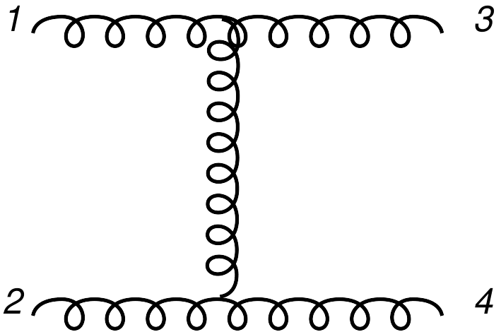
Figure 1: Example of a leading order Feynman diagram for the scattering process of four gluons.

The amplitude for the scattering of four gluons can be decomposed into different colour and Lorentz tensors. We begin by introducing our basis of tensor structures.

In order to define colour tensors with adjoint colour indices we introduce traces of fundamental generators $T^{a}_{ij}$. We abbreviate

$$tr(T^{a_{1}}T^{a_{2}}T^{a_{3}}T^{a_{4}})=tr(1234).$$ (9)

The vector of colour structures that we will use to express the amplitude is given by

$$\vec{c}^{~{}a_{1}a_{2}a_{3}a_{4}}_{gggg}=\left(\begin{array}[]{c}tr(1234)+tr(1432)\\ tr(1243)+tr(1342)\\ tr(1423)+tr(1324)\\ tr(12)tr(34)\\ tr(13)tr(24)\\ tr(14)tr(23)\\ \end{array}\right).$$ (10)

The Feynman integrand for our amplitude is a Lorentz tensor contracted with polarisation vectors $\epsilon^{\mu}_{i}(p_{i})$. In order to represent the Lorentz tensor we make an ansatz in terms of all $p_{i}^{\mu_{i}}$ and $g^{\mu_{i}\mu_{j}}$. Since we are considering an amplitude with four external gluons, our ansatz has tensor rank four. This yields in full generality 138 independent coefficients. To restrict ourselves to the physical subspace of the amplitude we choose a light-like axial gauge (see for example ref. Gehrmann:2013vga ) with the gauge conditions

$$\epsilon^{\mu}_{i}p_{i,\mu}=\epsilon^{\mu}_{i}p_{i-1,\mu}=0.$$ (11)

We identify $p_{0}^{\mu}=p_{4}^{\mu}$. In this gauge, the polarisation sum that has to be carried out to obtain squared matrix elements takes the form

$$\sum_{\text{polarisations}}\epsilon^{\mu}_{i}\epsilon^{*\,\nu}_{i}=g^{\mu\nu}-\frac{2}{s_{i,i-1}}\left(p_{i}^{\mu}p_{i-1}^{\nu}-p_{i}^{\nu}p_{i-1}^{\mu}\right).$$ (12)

Effectively, this polarisation sum annihilates every vector $p_{i}^{\mu}$ or $p_{i-1}^{\mu}$ in the amplitude. Only polarisations transverse to the two chosen vectors survive. We can anticipate the projection that would be performed when interfering the amplitude with its complex conjugate to produce squared matrix elements. We do so by replacing

$$\epsilon_{i}^{\mu}\rightarrow\left[g^{\mu\nu}-\frac{2}{s_{i,i-1}}\left(p_{i}^{\mu}p_{i-1}^{\nu}-p_{i}^{\nu}p_{i-1}^{\mu}\right)\right]\epsilon_{i}^{\nu}$$ (13)

in our ansatz for the general amplitude. This procedure effectively annihilates all but 20 tensor structures in our ansatz. After simple orthogonality checks we find that only 10 of the remaining structures are linearly independent. In order to represent those ten physical structures we define

$$P_{ij}^{\mu}=\frac{p_{j}^{\mu}}{s_{j,i}}-\frac{p_{i}^{\mu}s_{j,i-1}}{s_{i,i-1}s_{j,i}}-\frac{p_{i-1}^{\mu}}{s_{i,i-1}}$$ (14)

and

$$G_{ij}^{\mu\nu} = g^{\mu\nu}-\frac{2p_{i-1}^{\mu}p_{j}^{\nu}s_{j-1,i}}{s_{i,i-1}s_{j,j-1}}+\frac{2p_{i-1}^{\mu}p_{j-1}^{\nu}s_{j,i}}{s_{i,i-1}s_{j,j-1}}+\frac{2p_{i}^{\mu}p_{j}^{\nu}s_{j-1,i-1}}{s_{i,i-1}s_{j,j-1}}$$ (15)

$$+ \frac{2p_{i}^{\mu}p_{j-1}^{\nu}s_{j,i-1}}{s_{i,i-1}s_{j,j-1}}-\frac{2p_{i-1}^{\mu}p_{i}^{\nu}}{s_{i,i-1}}-\frac{2p_{i}^{\mu}p_{i-1}^{\nu}}{s_{i,i-1}}-\frac{2p_{j}^{\mu}p_{j-1}^{\nu}}{s_{j,j-1}}-\frac{2p_{j-1}^{\mu}p_{j}^{\nu}}{s_{j,j-1}}.$$

They satisfy separately our gauge conditions:

$$P_{ij}^{\mu}p_{i,\,\mu} = P_{ij}^{\mu}p_{i-1,\,\mu}=0\,,$$

$$G_{ij}^{\mu\nu}p_{i,\mu} = G_{ij}^{\mu\nu}p_{i-1,\mu}=0^{\nu}\,,$$

$$G_{ij}^{\mu\nu}p_{j,\nu} = G_{ij}^{\mu\nu}p_{j-1,\nu}=0^{\mu}.$$ (16)

We use the above definitions to define the 10 tensors as

$$\vec{T}^{\mu\nu\rho\sigma}_{gggg}=\left(\begin{array}[]{c}G_{12}^{\mu\nu}G_{34}^{\rho\sigma}\\ G_{13}^{\mu\rho}G_{24}^{\nu\sigma}\\ G_{14}^{\mu\sigma}G_{23}^{\nu\rho}\\ G_{12}^{\mu\nu}P^{\rho}_{31}P^{\sigma}_{42}\\ G_{13}^{\mu\rho}P^{\nu}_{24}P^{\sigma}_{42}\\ G_{14}^{\mu\sigma}P^{\nu}_{24}P^{\rho}_{31}\\ G_{23}^{\nu\rho}P^{\mu}_{13}P^{\sigma}_{42}\\ G_{24}^{\nu\sigma}P^{\mu}_{13}P^{\rho}_{31}\\ G_{34}^{\rho\sigma}P^{\mu}_{13}P^{\nu}_{24}\\ P^{\mu}_{13}P^{\nu}_{24}P^{\rho}_{31}P^{\sigma}_{42}\\ \end{array}\right).$$ (17)

We decompose the four gluon scattering amplitude as

$$\mathcal{A}_{gggg} = \epsilon^{\mu}_{a_{1}}(p_{1})\epsilon^{\nu}_{a_{2}}(p_{2})\epsilon^{\rho}_{a_{3}}(p_{3})\epsilon^{\sigma}_{a_{4}}(p_{4})\mathcal{A}_{gggg,\,\mu\nu\rho\sigma}^{a_{1}a_{2}a_{3}a_{4}}$$ (18)

$$= \epsilon^{\mu}_{a_{1}}(p_{1})\epsilon^{\nu}_{a_{2}}(p_{2})\epsilon^{\rho}_{a_{3}}(p_{3})\epsilon^{\sigma}_{a_{4}}(p_{4})\sum_{i=1}^{6}\sum_{j=1}^{10}c^{i,a_{1}a_{2}a_{3}a_{4}}_{gggg}T^{j}_{\mu\nu\rho\sigma,\,gggg}\mathcal{A}_{gggg}^{(i,j)}.$$

We refer to the coefficients $\mathcal{A}_{gggg}^{(i,j)}$ as scalar amplitude coefficients. Here, $\epsilon^{\mu}_{a}(p)$ is a polarisation vector with adjoint colour index $a$ corresponding to the gluon with momentum $p$.

Alternative to the representation of our amplitude introduced in eq. (18), it is useful to decompose our amplitude into different components according to the helicities of the external gluons. We can achieve this by projecting to two-dimensional external helicity states and by using the spinor-helicity framework (see for example ref. Dixon:1996wi ). Note, that the change of the dimension of external polarisation implies a change in the regularisation scheme used in the computation from CDR to HV scheme. The four-gluon scattering amplitude can then be written in this scheme as

$$\mathcal{A}_{gggg} = \epsilon_{a_{1}}\epsilon_{a_{2}}\epsilon_{a_{3}}\epsilon_{a_{4}}\sum_{i=1}^{6}\sum_{j=1}^{16}c^{i,a_{1}a_{2}a_{3}a_{4}}_{gggg}h^{j}_{gggg}\mathcal{A}_{gggg}^{\prime\,\,(i,j)}.$$ (19)

In the above equation the $\epsilon^{a_{i}}$ now simply label the colour of an external gluon. The 16 helicity configurations are represented by the following structures,

$$\vec{h}_{gggg} = \Bigg{\{}\frac{[21][43]}{\langle 12\rangle\langle 34\rangle},\frac{\langle 14\rangle[21][31]}{\langle 12\rangle\langle 13\rangle[41]},\frac{\langle 13\rangle[21][41]}{\langle 12\rangle\langle 14\rangle[31]},\frac{\langle 34\rangle[21]}{\langle 12\rangle[43]},\frac{\langle 23\rangle[31][43]}{\langle 13\rangle\langle 34\rangle[32]},\frac{\langle 14\rangle\langle 23\rangle[31]^{2}}{\langle 13\rangle^{2}[32][41]},$$ (20)

$$\frac{\langle 23\rangle[41]}{\langle 14\rangle[32]},\frac{\langle 23\rangle\langle 34\rangle[31]}{\langle 13\rangle[32][43]},\frac{\langle 13\rangle[32][43]}{\langle 23\rangle\langle 34\rangle[31]},\frac{\langle 14\rangle[32]}{\langle 23\rangle[41]},\frac{\langle 13\rangle^{2}[21][43]}{\langle 12\rangle\langle 34\rangle[31]^{2}},\frac{\langle 13\rangle\langle 14\rangle[21]}{\langle 12\rangle[31][41]},$$

$$\frac{\langle 12\rangle[43]}{\langle 34\rangle[21]},\frac{\langle 12\rangle\langle 14\rangle[31]}{\langle 13\rangle[21][41]},\frac{\langle 13\rangle\langle 23\rangle[43]}{\langle 34\rangle[31][32]},\frac{\langle 14\rangle\langle 23\rangle}{[32][41]}\Bigg{\}}.$$

The above helicity structures correspond to positive (+) or negative (-) helicity as in

$$\vec{h}_{gggg} \sim \{{----},{---+},{--+-},{--++},{-+--},{-+-+},{-++-},{-+++},$$ (21)

$${+---},{+--+},{+-+-},{+-++},{++--},{++-+},{+++-},{++++}\}\,.$$

Here, the $i^{th}$ sign in each element of the list correspond to the helicity of the parton with momentum $p_{i}$. The scalar coefficients of the amplitudes in the helicity basis can be written as a linear combination of the CDR amplitudes

$$\mathcal{A}_{gggg}^{\prime\,\,(i,j)}=\sum\limits_{k=1}^{10}T_{CDR\rightarrow\text{helicity},\,jk}\mathcal{A}_{gggg}^{(i,k)}.$$ (22)

We provide the above transformation matrix $T_{CDR\rightarrow\text{helicity}}$ and $\mathcal{A}_{gggg}$ in electronic form together with the arXiv submission of this article. Note, that only 8 of the scalar helicity amplitudes are independent due to charge conjugation symmetry. The projection from CDR to HV is thus not invertible.

4 The Two-Gluon and Two-Quark Amplitudes

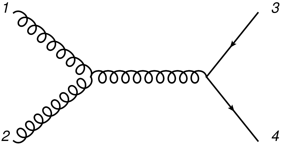
Figure 2: Example of a leading order Feynman diagram for the scattering process of two gluons and two quarks.

The amplitude for the scattering of two gluons and two quarks can be decomposed into colour and Lorentz tensor structures. The basis of colour structures for the amplitudes for the scattering of two gluons and two quarks can be brought in the form

$$\vec{c}_{ggq\bar{q}}=\left(\begin{array}[]{c}\delta^{a_{1}a_{1}}\delta_{i_{4}i_{3}}\\ T^{a_{2}}_{i_{4}i_{5}}T^{a_{1}}_{i_{5}i_{3}}\\ T^{a_{1}}_{i_{4}i_{5}}T^{a_{2}}_{i_{5}i_{3}}\\ \end{array}\right).$$ (23)

To derive the Lorentz tensor structures to represent our amplitude we begin with the following considerations. In order to remove unphysical redundancies similar to the four gluon scattering case we work in a gauge where

$$\epsilon(p_{1}).p_{1}=\epsilon(p_{1}).p_{2}=\epsilon(p_{2}).p_{1}=\epsilon(p_{2}).p_{2}=0.$$ (24)

Owing to the momentum conservation we have $\bar{u}(p_{3})\not{p}_{2}u(p_{4})=-\bar{u}(p_{3})\not{p}_{1}u(p_{4})$. Applying this identity and exploiting the restrictions imposed by the gauge choice we find that we can choose the following spinor and Lorentz structures as a basis to represent our amplitude

$$\vec{T}^{\mu\nu}_{ggq\bar{q}}=\left(\begin{array}[]{c}\Gamma^{\mu\nu}_{\perp}\\ \not{p}_{1}g_{\perp}^{\mu\nu}\\ \not{p}_{1}(P_{3}^{\mu}P_{3}^{\nu}-P_{4}^{\mu}P_{3}^{\nu}-P_{4}^{\mu}P_{3}^{\nu}+P_{4}^{\mu}P_{4}^{\nu})\\ \gamma^{\mu}_{\perp}(P_{3}^{\nu}-P_{4}^{\nu})\\ \gamma^{\nu}_{\perp}(P_{3}^{\mu}-P_{4}^{\mu})\end{array}\right).$$ (25)

Here, we use the definitions

$$\Gamma^{\mu\nu}_{\perp} = s_{12}\gamma^{\mu}\not{p}_{1}\gamma^{\nu}+2s_{13}\gamma^{\nu}p_{1}^{\mu}+2s_{23}\gamma^{\mu}p_{1}^{\mu}$$

$$- 4\not{p}_{1}\left(p_{1}^{\mu}p_{1}^{\nu}+p_{1}^{\mu}p_{3}^{\nu}+p_{1}^{\nu}p_{4}^{\nu}\right)\,,$$

$$g_{\perp}^{\mu\nu} = g^{\mu\nu}-\frac{2}{s_{12}}(p_{1}^{\mu}p_{2}^{\nu}+p_{2}^{\mu}p_{1}^{\nu})\,,$$

$$\gamma_{\perp}^{\mu} = \gamma^{\mu}+\not{p}_{1}\frac{2}{s_{12}}(p_{1}^{\mu}-p_{2}^{\mu})\,,$$

$$P_{i}^{\mu} = s_{12}p_{i}^{\mu}-s_{2i}p_{1}^{\mu}-s_{1i}p_{2}^{\mu}\,.$$ (26)

With this we may finally write the amplitude as

$$\mathcal{A}_{ggq\bar{q}}=\epsilon_{\mu}^{a_{1}}(p_{1})\epsilon_{\nu}^{a_{2}}(p_{2})\sum\limits_{i=1}^{3}\sum\limits_{j=1}^{5}\bar{u}_{b_{4}}(p_{4})c^{i,\,a_{1}a_{2}}_{b_{4}b_{3},\,ggq\bar{q}}T^{j,\,\mu\nu}_{ggq\bar{q}}u_{b_{3}}(p_{3})\mathcal{A}^{(i,j)}_{ggq\bar{q}}.$$ (27)

Furthermore, we may decompose our amplitude in components that correspond to different helicities of the external particles. In this decomposition, we write

$$\mathcal{A}_{ggq\bar{q}}=\epsilon^{a_{1}}\epsilon^{a_{2}}\bar{v}^{b_{4}}v^{b_{3}}\sum\limits_{i=1}^{3}\sum\limits_{j=1}^{8}c^{i,\,a_{1}a_{2}}_{b_{4}b_{3},\,ggq\bar{q}}h^{j}_{ggq\bar{q}}\mathcal{A}^{\prime\,(i,j)}_{ggq\bar{q}}.$$ (28)

The vectors $\bar{v}^{b_{4}}$ and $v^{b_{3}}$ carry the colour indices of the external anti-quark and quark. The individual helicity structures are given by

$$\vec{h}_{ggq\bar{q}} = \Big{\{}\frac{\langle 14\rangle[21][31]}{\langle 12\rangle},\frac{\langle 13\rangle[21][41]}{\langle 12\rangle},\frac{\langle 23\rangle\langle 24\rangle[31]}{\langle 13\rangle},\frac{\langle 23\rangle\langle 24\rangle[41]}{\langle 14\rangle},\frac{\langle 14\rangle[32][42]}{[41]},$$ (29)

$$\frac{\langle 13\rangle\langle 14\rangle[42]}{\langle 24\rangle},\frac{\langle 12\rangle\langle 14\rangle[31]}{[21]},\frac{\langle 12\rangle\langle 13\rangle[41]}{[21]}\Big{\}}.$$

The above helicity structures correspond to positive and negative helicities as in

$$\vec{h}_{ggq\bar{q}}\sim\{{---+},{--+-},{-+-+},{-++-},{+--+},{+-+-},{++-+},{+++-}\}.$$ (30)

Here, the $i^{th}$ sign in each element of the list correspond to the helicity of the parton with momentum $p_{i}$. Similarly to eq. (22) in the case of the four gluon amplitude, the scalar amplitude coefficients in the spinor-helicity representation can be written as a linear combination of the CDR amplitude coefficients. We provide this linear relation in electronic form together with the arXiv submission of this article.

Our scalar four particle amplitude is constructed such that if we consider the scattering kinematics of $p_{1}\,p_{2}\rightarrow p_{3}\,p_{4}$ all HPLs are real and the variable $x\in[0,1]$. Of course, this is not the only scattering process of a pair of quarks and gluons that can be considered. To obtain for example the amplitudes for the scattering of a quark and a gluon into a quark and a gluon we have to consider the kinematics of $p_{1}\,p_{3}\rightarrow p_{2}\,p_{4}$. While the permutation of external momenta in the tensor structures in eq. (25) and eq. (29) is trivial analytically continuing the HPLs in the scalar amplitudes is not. How to perform this analytic continuation was discussed for example in ref. Henn:2019rgj and we provide a brief summary in appendix A.

5 Four-Quark Amplitude

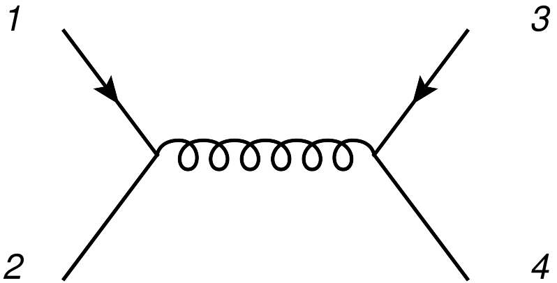
Figure 3: Leading order Feynman diagram for the scattering process of four quarks.

In the case of scattering amplitudes of four quarks we have to distinguish the case where all four quarks have the same flavour or two pairs of different flavours are scattering. We refer to the scattering amplitude of the latter case as $\mathcal{A}_{q\bar{q}Q\bar{Q}}$. The former amplitude can then be expressed as

$$\mathcal{A}_{q\bar{q}q\bar{q}}(p_{1},p_{2},p_{3},p_{4})=\mathcal{A}_{q\bar{q}Q\bar{Q}}(p_{1},p_{2},p_{3},p_{4})-\mathcal{A}_{q\bar{q}Q\bar{Q}}(p_{1},p_{4},p_{3},p_{2}).$$ (31)

In the above equation we explicitly wrote the dependence of the amplitudes on the momenta to illustrate which momenta have to be exchanged in order to satisfy the relation.

The amplitude for the scattering of two quark- and anti-quark pairs of different flavours can be decomposed into colour and Lorentz structures as

$$\mathcal{A}_{q\bar{q}Q\bar{Q}}=\sum\limits_{i=1}^{2}\sum\limits_{j=1}^{\infty}c^{i}_{q\bar{q}Q\bar{Q}}T^{j}_{q\bar{q}Q\bar{Q}}\mathcal{A}^{(i,j)}_{q\bar{q}Q\bar{Q}}.$$ (32)

In order to define the colour factors $c^{i}_{q\bar{q}Q\bar{Q}}$ and spinor structures $T^{j}_{q\bar{q}Q\bar{Q}}$ in the above equation, we find it convenient to decompose a spinor $u_{i}^{a}(p)$ with a fundamental colour index $a$ and spinor index $i$ into two factors

$$u_{i}^{a}(p)=u_{i}(p)v^{a}.$$ (33)

The purpose of the vector $v^{a}$ is purely to label the colour of the external quark and $u_{i}(p)$ is a four component spinor. The basis of colour structures for the amplitudes can be brought in the form

$$\vec{c}_{q\bar{q}Q\bar{Q}}=\left(\begin{array}[]{c}\bar{v}^{a_{1}}\delta_{a_{1}a_{2}}v^{a_{2}}\times\bar{v}^{a_{3}}\delta_{a_{3}a_{4}}v^{a_{4}}\\ \bar{v}^{a_{1}}\delta_{a_{1}a_{4}}v^{a_{4}}\times\bar{v}^{a_{3}}\delta_{a_{3}a_{2}}v^{a_{2}}\\ \end{array}\right).$$ (34)

The spinor structures can be written in terms of the following basis.

$$\vec{T}_{q\bar{q}Q\bar{Q}}=\left(\begin{array}[]{c}\bar{u}(p_{2})\not{p}_{3}u(p_{1})\times\bar{u}(p_{4})\not{p}_{1}u(p_{3})\\ \bar{u}(p_{2})\gamma^{\mu}u(p_{1})\times\bar{u}(p_{4})\gamma_{\mu}u(p_{3})\\ \bar{u}(p_{2})\not{p}_{3}\gamma^{\mu}\gamma^{\nu}u(p_{1})\times\bar{u}(p_{4})\not{p}_{1}\gamma_{\mu}\gamma_{\nu}u(p_{3})\\ \bar{u}(p_{2})\gamma^{\mu}\gamma^{\nu}\gamma^{\rho}u(p_{1})\times\bar{u}(p_{4})\gamma_{\mu}\gamma_{\nu}\gamma_{\rho}u(p_{3})\\ \bar{u}(p_{2})\not{p}_{3}\gamma^{\mu}\gamma^{\nu}\gamma^{\rho}\gamma^{\sigma}u(p_{1})\times\bar{u}(p_{4})\not{p}_{1}\gamma_{\mu}\gamma_{\nu}\gamma_{\rho}\gamma_{\sigma}u(p_{3})\\ \bar{u}(p_{2})\gamma^{\mu}\gamma^{\nu}\gamma^{\rho}\gamma^{\sigma}\gamma^{\tau}u(p_{1})\times\bar{u}(p_{4})\gamma_{\mu}\gamma_{\nu}\gamma_{\rho}\gamma_{\sigma}\gamma_{\tau}u(p_{3})\\ \dots\end{array}\right).$$ (35)

Depending on the loop order we require more and more $\gamma$ matrices between the spinors. Specifically, to express the $L$- loop amplitude $2L-1$ $\gamma$-matrices are maximally required as soon as $L\geq 2$ (see for example ref. Glover:2004si ).

Furthermore, we may decompose our amplitude in components that correspond to different helicities of the external particles. We find

$$\mathcal{A}_{q\bar{q}Q\bar{Q}}=\sum\limits_{i=1}^{2}\sum\limits_{j=1}^{4}c^{i}_{q\bar{q}Q\bar{Q}}h^{j}_{q\bar{q}Q\bar{Q}}\mathcal{A}^{\prime\,(i,j)}_{q\bar{q}Q\bar{Q}}.$$ (36)

Here the helicity basis is spanned by

$$\vec{h}_{q\bar{q}Q\bar{Q}}=\Big{\{}\frac{\langle 14\rangle\langle 23\rangle[31]}{\langle 13\rangle},\langle 14\rangle[32],\langle 23\rangle[41],\frac{\langle 13\rangle[21][43]}{[31]}\Big{\}}.$$ (37)

The above helicity structures correspond to positive and negative helicities as in

$$\vec{h}_{q\bar{q}Q\bar{Q}}\sim\{{-+-+},{-++-},{+--+},{+-+-}\}.$$ (38)

Here, the $i^{th}$ sign in each element of the list correspond to the helicity of the parton with momentum $p_{i}$. Similarly to eq. (22) in the case of the four gluon amplitude, the scalar amplitude coefficients in the spinor-helicity representation can be written as a linear combination of the CDR amplitude coefficients. We provide this linear relation in electronic form together with the arXiv submission of this article.

The variables in our amplitudes are chosen such that in the kinematic region of scattering particles with momenta $p_{1}$ and $p_{2}$ into particles with momenta $p_{3}$ and $p_{4}$ all HPLs are real and our variable $x\in[0,1]$. However, this is just one particular case of scattering two quarks of each other and we may consider any permutation of momenta to cover all possible four quark scattering processes. While obtaining such a permutation on the spinor structures of eq. (35) and eq. (37) is relatively simple the analytic continuation of the HPLs in our scalar amplitude coefficients is non-trivial. How such an analytic continuation can be obtained was discussed for example in ref. Henn:2019rgj and we outline it explicitly for convenience in appendix A.

6 Ultraviolet and Infrared Structure

In this section, we review the structure of the poles in the dimensional regulator appearing in the four-point scattering amplitudes. The coefficients of the poles are well understood and can be expressed at least up to third order as products of known, universal factors and lower loop amplitudes. Singularities arise due to soft (infrared) or collinear divergences of the loop integrands or due to ultraviolet (infinite momentum) divergences. The possibility to derive the poles of an amplitude by direct computation serves as a stringent test of our computation. Not surprisingly we find agreement of our amplitudes with the structure of singularities outlined below.

Ultraviolet divergences in massless QCD scattering amplitudes can be universally reabsorbed into a renormalisation of the strong coupling constant. The renormalisation factor $Z$ can be derived by regarding the renormalisation group equation for $a_{R}$ (eq. (2)):

$$\frac{\partial}{\partial\log(\mu^{2})}a_{R}(\mu^{2})=-\epsilon a_{R}(\mu^{2})+a_{R}\beta.$$ (39)

The $\beta$-function is related to the renormalisation factor $Z$ by

$$\beta=-\frac{\partial\log(Z)}{\partial\log(\mu^{2})}=a_{R}\sum\limits_{i=0}^{\infty}a_{R}^{i}\beta_{i}.$$ (40)

Solving the above evolution equation we can derive

$$Z=1+\frac{a_{R}\beta_{0}}{\epsilon}+a_{R}^{2}\left(\frac{\beta_{0}^{2}}{\epsilon^{2}}+\frac{\beta_{1}}{2\epsilon}\right)+a_{R}^{3}\frac{\left(2\beta_{2}\epsilon^{2}+7\beta_{1}\beta_{0}\epsilon+6\beta_{0}^{3}\right)}{6\epsilon^{3}}+\mathcal{O}(a_{R}^{4}).$$ (41)

The QCD $\beta$-function coefficients are currently known to five-loop order Herzog:2017 ; Baikov:2016 . We only require the first two for the purposes of this article which read

$$\beta_{0} = -\frac{1}{4}\left(\frac{11}{3}C_{A}-\frac{2}{3}n_{f}\right)\,,$$

$$\beta_{1} = -\frac{1}{16}\left(\frac{34}{3}C_{A}^{2}-\frac{10}{3}C_{A}n_{f}-2C_{F}n_{f}\right).$$ (42)

The quadratic Casimirs in adjoint and fundamental representations are denoted by $C_{A}=n_{c}$ and $C_{F}=(n_{c}^{2}-1)/2n_{c}$, respectively.

In general, a renormalised amplitude for the scattering of $n$ massless, SU($n_{c})$ colour charged fields in dimensional regularisation can be written as

$$\mathcal{A}_{n}(\{p_{i}\},\epsilon)=\mathbf{Z}_{n}(\{p_{i}\},\epsilon)\mathcal{A}_{n}^{f}(\{p_{i}\},\epsilon)\,.$$ (43)

Here $\mathcal{A}_{n}^{f}(\{p_{i}\})$ represents a finite hard amplitude depending on the the momenta $p_{i}$, colours and spins of the external states. The factor $\mathbf{Z}_{n}(\{p_{i}\},\epsilon)$ is universal and contains all infrared divergences Catani:1998bh ; Sterman:2002qn ; Aybat:2006wq ; Aybat:2006mz ; Becher:2009cu ; Gardi:2009qi ; Almelid:2015jia ; Almelid:2017qju . To indicate an operator in colour space we use bold letters. $\mathbf{Z}_{n}(\{p_{i}\},\epsilon)$ is given explicitly by the exponential

$$\mathbf{Z}_{n}(\{p_{i}\},\epsilon)=\mathcal{P}exp\left\{-\frac{1}{4}\int_{0}^{\mu^{2}}\frac{d\mu^{2}}{\mu^{2}}\mathbf{\Gamma}_{n}(\{p_{i}\},\mu^{2},a_{R}(\mu^{2}))\right\}.$$ (44)

The soft anomalous dimension for $n$ fields is then given by

$$\mathbf{\Gamma}_{n}(\{p_{i}\},\mu^{2},a_{R})=\mathbf{\Gamma}^{\text{dip.}}_{n}(\{p_{i}\},\mu^{2},a_{R})+\mathbf{\Delta}(\{\rho_{ijkl}\}).$$ (45)

The first term on the right-hand side of the above equation corresponds to radiation from colour dipoles

$$\mathbf{\Gamma}^{\text{dip.}}_{n}(\{p_{i}\},\mu^{2},a_{R})=-\frac{1}{2}\gamma_{c}(a_{R})\sum\limits_{i\neq j}^{n}\mathbf{T}_{i}\cdot\mathbf{T}_{j}\log\left(\frac{-s_{ij}}{\mu^{2}}\right)+\mathbf{\mathbb{I}}\sum\limits_{J=1}^{n}\gamma_{J}(a_{R}).$$ (46)

The operator $\mathbf{T}_{i}$ is commonly referred to as colour charge operator. The action of such a colour charge operator on a scattering amplitude is given by regarding its action on individual spinors or polarisation vectors contracted with an amplitude

$$\mathbf{T}^{a}_{i}\circ\epsilon^{b}_{\mu}(p_{i})\mathcal{A}^{\mu}_{b} = -if^{abc}\epsilon^{\mu}_{b}(p_{i})\mathcal{A}_{\mu,\,c}\,,$$

$$\mathbf{T}^{a}_{i}\circ\mathcal{A}_{j,\,b}u_{j,\,b}(p_{i}) = \mathcal{A}_{j,\,b}T^{a}_{bc}u_{j,\,c}(p_{i}).$$ (47)

Here, $f^{abc}$ is SU($n_{c}$) structure constant and $T^{a}_{bc}$ is a fundamental generator. We introduce the abbreviation

$$\mathbf{D}(\mu^{2})=\sum\limits_{i>j=1}^{n}\mathbf{T}_{i}\cdot\mathbf{T}_{j}\log\left(\frac{-s_{ij}}{\mu^{2}}\right),\hskip 28.45274pt\mathbf{D}_{0}=\sum\limits_{i>j=1}^{n}\mathbf{T}_{i}\cdot\mathbf{T}_{j}.$$ (48)

$\gamma_{c}$ is the cusp anomalous dimension and $\gamma_{J}$ are the anomalous dimensions associated with the external fields. The second term on the right hand side of eq. (45) allows for soft radiation that relates more than two colour charged partons. The correction to the dipole formula Almelid:2015jia ; Almelid:2017qju starts at third order in the coupling constant, and will therefore not be needed in the present paper.

With this we now know the entire dependence of $\Gamma_{n}$ on the artificial scale $\mu^{2}$. Specifically, $\Gamma_{n}$ depends on $\mu^{2}$ only via a single logarithm and indirectly via $a_{R}$. Carrying out the $\mu^{2}$-integral explicitly we find

$$- \frac{1}{2}\int_{0}^{\mu^{2}}\frac{d\mu^{2}}{\mu^{2}}\mathbf{\Gamma}^{\text{dip.}}_{n}(\{p_{i}\},\mu^{2},a_{R}(\mu^{2}))=a_{R}\left[\frac{\gamma_{c}^{(1)}}{8\epsilon^{2}}\mathbf{D}_{0}-\frac{\gamma_{c}^{(1)}}{8\epsilon}\mathbf{D}+\sum\limits_{J=1}^{n}\frac{\gamma_{J}^{(1)}}{2\epsilon}\mathbf{\mathbb{I}}\right]$$

$$+ a_{R}^{2}\left[\left(\frac{\beta_{0}\gamma_{c}^{(1)}}{32\epsilon^{3}}+\frac{\gamma_{c}^{(2)}}{32\epsilon^{2}}\right)\mathbf{D}_{0}+\left(-\frac{\beta_{0}\gamma_{c}^{(1)}}{16\epsilon^{2}}-\frac{\gamma_{c}^{(2)}}{16\epsilon}\right)\mathbf{D}+\sum\limits_{J=1}^{n}\left(\frac{\beta_{0}\gamma_{J}^{(1)}}{\epsilon^{2}}+\frac{\gamma_{J}^{(2)}}{4\epsilon}\right)\mathbf{\mathbb{I}}\right]+\mathcal{O}(a_{R}^{3}).$$

Here, we expanded the anomalous dimensions in the strong coupling constant.

$$\gamma_{c}(a_{R})=\sum\limits_{i=1}^{\infty}a_{R}^{i}\gamma_{c}^{(i)},\hskip 28.45274pt\gamma_{J}(a_{R})=\sum\limits_{i=1}^{\infty}a_{R}^{i}\gamma_{J}^{(i)}.$$ (50)

The first two terms in the expansion of the cusp anomalous dimensions are given by

$$\gamma_{c}^{(1)} = 1\,,$$

$$\gamma_{c}^{(2)} = C_{A}\left(\frac{67}{36}-\frac{1}{2}\zeta_{2}\right)-\frac{5}{18}n_{f}.$$ (51)

The first two terms in the expansion of the collinear anomalous dimensions are given by

$$\gamma_{g}^{(1)} = -\frac{11}{12}C_{A}+\frac{1}{6}n_{f},$$

$$\gamma_{q}^{(1)} = -\frac{3}{4}C_{F},$$

$$\gamma_{g}^{(2)} = C_{A}^{2}\left(-\frac{173}{108}+\frac{11\pi^{2}}{288}+\frac{\zeta_{3}}{8}\right)+C_{A}n_{f}\left(\frac{8}{27}-\frac{\pi^{2}}{144}\right)+\frac{1}{8}C_{F}n_{f}\,,$$

$$\gamma_{q}^{(2)} = C_{A}C_{F}\Big{(}-\frac{961}{864}-\frac{11\pi^{2}}{96}+\frac{13\zeta_{3}}{8}\Big{)}+C_{F}^{2}\Big{(}-\frac{3}{32}+\frac{\pi^{2}}{8}-\frac{3\zeta_{3}}{2}\Big{)}$$ (52)

$$+C_{F}n_{f}\Big{(}\frac{65}{432}+\frac{\pi^{2}}{48}\Big{)}\,.$$

7 Checks on Results

We perform a number of consistency checks on the scattering amplitudes to ensure the correctness of our result.

• As described in section 2, all amplitudes were generated by two independent calculational setups.

• All four-point scattering amplitudes exhibit the universal infrared structures predicted by eq. (44). This serves as the most stringent check on our results.

• The four-gluon helicity amplitudes are consistent with the existing results computed in ref. Bern:2002tk to ${\cal O}(\epsilon^{0})$. Moreover, interfering the CDR amplitude with its tree level equivalent reproduces correctly the results of ref. Glover:2001af .

• We explicitly checked that only 4 helicity amplitudes ($++++,-+++,--++,-+-+$) for four gluon scattering are independent (as dictated by Bose, parity and time-reversal symmetry).

• The one-loop U(1) decoupling identity Bern:1990ux for the four-gluon amplitude is satisfied. This identity states that the double trace coefficients of the pure gauge part of the four-gluon amplitude for any helicity configuration should be related to the corresponding single trace elements through

  $${\cal A}_{gggg}^{\prime(4,j,1)}={\cal A}_{gggg}^{\prime(5,j,1)}={\cal A}_{gggg}^{\prime(6,j,1)}=\frac{2}{n_{c}}\Big{(}{\cal A}_{gggg}^{\prime(1,j,1)}+{\cal A}_{gggg}^{\prime(2,j,1)}+{\cal A}_{gggg}^{\prime(3,j,1)}\Big{)}\,.$$ (53)

  In the above equation, the quantity ${\cal A}_{gggg}^{\prime\,(i,j,k)}$ is defined through

  $${\cal A}_{gggg}^{\prime\,(i,j)}=\frac{\alpha}{4\pi}\sum_{k=0}^{\infty}\left(\frac{\alpha}{4\pi}\right)^{k}{\cal A}_{gggg}^{\prime\,(i,j,k)}\,,$$ (54)

  where ${\cal A}_{gggg}^{\prime\,(i,j)}$ is introduced in eq. (19).

  Moreover, in ref. Naculich:2011ep , more general group theory constraints are discussed which are also verified for the two-loop helicity amplitudes. In order to present those, we rewrite the $n_{f}$ independent part of the four gluon amplitude in eq. (19) as

  $$\mathcal{A}_{gggg}= \epsilon_{a_{1}}\epsilon_{a_{2}}\epsilon_{a_{3}}\epsilon_{a_{4}}\sum_{i=1}^{3}\sum_{j=1}^{16}\sum_{k=0}^{\infty}\sum_{m=0}^{\lfloor\frac{k}{2}\rfloor}n_{c}^{k-2m}c^{i,a_{1}a_{2}a_{3}a_{4}}_{gggg}h^{j}_{gggg}\left(\frac{\alpha_{s}}{4\pi}\right)^{k+1}\mathcal{A}_{gggg}^{\prime\,(i,j,k,2m)}\,$$

  $$+ \epsilon_{a_{1}}\epsilon_{a_{2}}\epsilon_{a_{3}}\epsilon_{a_{4}}\sum_{i=4}^{6}\sum_{j=1}^{16}\sum_{k=0}^{\infty}\sum_{m=0}^{\lfloor\frac{k-1}{2}\rfloor}n_{c}^{k-2m-1}c^{i,a_{1}a_{2}a_{3}a_{4}}_{gggg}h^{j}_{gggg}\left(\frac{\alpha_{s}}{4\pi}\right)^{k+1}\mathcal{A}_{gggg}^{\prime\,(i,j,k,2m+1)}\,.$$ (55)

  The constraints take the form

  $$\sum_{i=1}^{3}{\cal A}_{gggg}^{\prime(i,j,2,2)}=0\,,$$

  $$6\sum_{i=1}^{3}{\cal A}_{gggg}^{\prime(i,j,2,0)}-\sum_{i=4}^{6}{\cal A}_{gggg}^{\prime(i,j,2,1)}=0\,,$$

  $${\cal A}_{gggg}^{\prime(i,j,2,2)}+{\cal A}_{gggg}^{\prime((i+4)~{}{\rm modulo}~{}6,j,2,1)}={\text{independent of }}i\,.$$ (56)

• We find complete agreement with ref. Bern:2003ck for the one- and two-loop helicity amplitudes for the two-gluon and two-quark channel.

• We find that one- and two-loop helicity amplitudes for four-quark scattering with two different flavours are in agreement with the existing results computed in ref. DeFreitas:2004kmi .

  Note that in the aforementioned references Bern:2002tk ; Bern:2003ck ; DeFreitas:2004kmi , the finite remainder is defined through subtraction operators which are different from the ones used in this article at ${\cal O}(\epsilon^{0})$. The difference is taken into account while performing the comparison.

8 Conclusions

As a main result of this article, we provide the scalar amplitude coefficients of the four-particle scattering amplitudes in CDR together with the arXiv submission of the article. We include the LO, NLO and NNLO coefficients computed to sixth, fourth and second power in the Laurent expansion in the dimensional regulator respectively in machine readable form. Furthermore, we include the transformation matrices $T_{CDR\rightarrow\text{helicity}}$ to easily extract the amplitudes coefficients in the spinor-helicity basis.

Our result represents the first step towards a computation of three-loop, four-parton scattering amplitudes in QCD. In particular, our results can be used to predict the infrared and collinear pole structure of such three loop amplitudes. Furthermore, they are a necessary ingredient to obtain a suitable ultraviolet, infrared and collinear subtraction term for future cross section computations.

Terms beyond the finite order in the dimensional regulator are obtained in this article for the first time. Beyond their application to future collider phenomenology these terms may serve as analytic data for the analysis of QCD scattering amplitudes, such as the Regge limit. Our amplitudes are represented in the form of widely used harmonic polylogarithms in a uniform notation which makes their application and analysis simple.

With this work we have taken a very first step towards the formidable task of computing one of the most crucial collider processes - the production of two hadronic jets - to third order in QCD perturbation theory.

Appendix A Permutation of External Momenta

The results for the four point scattering amplitude of this paper are presented such that in the particular kinematic region of particles with momenta $p_{1}$ and $p_{2}$ scattering into particles $p_{3}$ and $p_{4}$ all HPLs are real valued and the evaluation of our amplitudes is straight forward. However, this particular scattering region is not the only scattering region of interest. For example, relating our amplitudes to the case of particles with momentum $p_{1}$ and $p_{3}$ scattering into particles with momentum $p_{2}$ and $p_{4}$ is non-trivial. Consequently, it is useful to describe how such a relation can be achieved. Mainly we have to concern ourselves with the transformation of HPLs from one scattering region to the other. How this can be achieved was described for example in ref. Henn:2019rgj but we find it convenient to outline the basic steps here.

First, it is prudent to recall that all our L-loop amplitudes have a pre-factor

$$\left(\frac{s_{12}}{\mu^{2}}\right)^{-L\epsilon}=1-L\epsilon\log\left(\frac{s_{12}}{\mu^{2}}\right)+\mathcal{O}(\epsilon^{2}).$$ (57)

Naturally, this pre-factor needs to be taken into account when permutaions of external legs are performed. Furthermore, it is necessary to restore the correct energy dimension of the scalar amplitudes since we chose for convenience $s_{12}=1$ in our results. While the permutation of external legs is obvious for tensor and helicity structures, this is not the case for the analytic functions appearing in our amplitudes. Let us first consider the permutation where momentum $p_{1}$ and $p_{2}$ are exchanged. This leaves the Mandelstam invariant $s_{12}$ invariant and exchanges $s_{13}$ and $s_{23}$ and replaces $x\rightarrow 1-x$. In the scattering region we used to define our amplitudes both $s_{13}$ and $s_{23}$ are negative and no branch cut of our amplitude is crossed by performing this permutation. Transforming the HPLs can be done by standard methods (see for example ref. Maitre:2005uu ) and does not introduce new imaginary parts.

If we consider scattering kinematics where a Mandelstam invariant changes its sign (for example $s_{12}<0$) we need to analytically continue the HPLs of our amplitudes. To achieve this we may attribute an infinitesimally small imaginary part to each Lorentz invariant scalar product of momenta:

$$s_{12} \rightarrow s_{12}-i0\,,$$ (58)

$$s_{13} \rightarrow s_{13}-i0\,,$$

$$s_{23} \rightarrow s_{23}-i0\,.$$

However, in our calculation we applied the relation $s_{12}+s_{13}+s_{23}=0$ which arises due to momentum conservation. As a consequence the above assignment cannot be done uniquely and it is ambiguous which infinitesimal phase should be attributed to the variable x. For example, consider two different possibilities of thinking about the polynomial $1-x$.

1. $$1-x=-\frac{s_{23}-i0}{s_{12}-i0}=-\frac{s_{23}}{s_{12}}+i0.$$ (59)

2. $$1-x=1+\frac{s_{13}-i0}{s_{12}-i0}=1+\frac{s_{13}}{s_{12}}-i0.$$ (60)

In the above equations the sign of the infinitesimal imaginary part differs, which demonstrates the problematic ambiguity. To perform an analytic continuation from one scattering region to another after having applied the momentum conservation identity we need to add another bit of information. The branch cuts of our scattering amplitude are located at kinematic points where Mandelstam invariants vanish. If we can manifest the branch cuts of our amplitude in terms of explicit logarithms we can easily identify the argument of these logarithms as being ratios of Mandelstam invariants. We discuss how this can be achieved at hands of a specific example below.

We consider the permutation of momenta $p_{2}\leftrightarrow p_{3}$. We find that our variable $x$ changes:

$$x=-\frac{(p_{1}+p_{3})^{2}}{(p_{1}+p_{2})^{2}}\rightarrow-\frac{(p_{1}+p_{2})^{2}}{(p_{1}+p_{3})^{2}}=\frac{1}{y}\,.$$ (61)

In the new, desired scattering region $p_{1}\,p_{3}\rightarrow p_{2}\,p_{4}$ we find $y\in[0,1]$. However, we need to be careful when transforming the logarithmic branch cuts of our amplitude.

$$\log(s_{12}-i0)\rightarrow\log(s_{13}-i0) = \log(s_{12}-i0)+\log\left(\frac{-s_{13}+i0}{s_{12}-i0}\right)-i\pi$$

$$= \log(s_{12}-i0)+\log\left(y\right)-i\pi.$$

$$\log(x)=\log\left(\frac{-s_{13}+i0}{s_{12}-i0}\right) \rightarrow -\log(y)+2i\pi.$$

$$\log(1-x)=\log\left(\frac{-s_{23}+i0}{s_{12}-i0}\right) \rightarrow \log(1-y)-\log(y)+i\pi.$$ (62)

All branch points of our amplitudes are located at $x=0$, $x=1$ and $x=\infty$. As we can see from the above equations all three branch cuts are crossed when the desired permutation is performed. This complicates the transformation of HPLs and we discuss our solution in the following. Our amplitudes are comprised of HPLs and consequently only one branch cut can be made manifest in terms of explicit logarithms at a time. In particular, this can be achieved by shuffle identities of the HPL’s such as

$$H(a_{n},\dots,a_{2},0,x)=H(a_{n},\dots,a_{2},x)\log(x)-H(0,a_{n},\dots,a_{2},x)-\dots-H(a_{n},\dots,0,a_{2},x)$$ (63)

or generalisations thereof, that make branch cuts (here at $x=0$) explicit. In order to perform the permutation corresponding to the exchange of momenta $p_{2}\leftrightarrow p_{3}$ we proceed in three sequential steps. In each of the steps only one branch cut at $x=0$ or $x=1$ is crossed. This implies that we may use shuffle identities to make the branch cut in our amplitude explicit and that the transformation of the remaining HPLs at each step does not introduce any imaginary parts. The three steps are given by the following.

1. Analytically continue into a scattering region where $s_{12}^{\prime}>0$, $s_{13}^{\prime}>0$ and $s_{23}^{\prime}<0$ and define $x^{\prime}=-x$.

   $$\log(s_{12}-i0) \rightarrow \log(s_{12}^{\prime}-i0).$$

   $$\log(x) \rightarrow \log(x^{\prime})+i\pi.$$

   $$\log(1-x) \rightarrow \log(1+x^{\prime}).$$ (64)

2. Permute the external momenta $p_{2}\leftrightarrow p_{3}$ and introduce $x^{\prime\prime}=\frac{1}{x^{\prime}}$.

   $$\log(s_{12}^{\prime}-i0) \rightarrow \log(s_{12}^{\prime\prime}-i0)+\log\left(x^{\prime\prime}\right).$$

   $$\log(x^{\prime}) \rightarrow -\log(x^{\prime\prime}).$$

   $$\log(1+x^{\prime}) \rightarrow \log(1+x^{\prime\prime})-\log(x^{\prime\prime}).$$

3. Analytically continue into a scattering region where $s_{12}^{\prime\prime\prime}>0$, $s_{13}^{\prime\prime\prime}<0$ and $s_{23}^{\prime\prime\prime}<0$ and define $x^{\prime\prime\prime}=-x^{\prime\prime}$.

   $$\log(s_{12}^{\prime\prime}-i0) \rightarrow \log(s_{12}^{\prime\prime\prime}-i0).$$

   $$\log(x^{\prime\prime}) \rightarrow \log(x^{\prime\prime\prime})-i\pi.$$

   $$\log(1+x^{\prime\prime}) \rightarrow \log(1-x^{\prime\prime\prime}).$$ (66)

Having completed the three transformations we performed the desired permutation and may drop the ^′ labels for convenience.

Finally, we note that any other permutation of external legs can simply be a sequence of the two example permutations outlined above. With this we showed how to obtain the four-point scattering amplitude for any scattering kinematics starting from the amplitudes provided in this article.

References

- (1) ATLAS collaboration, Measurement of inclusive jet and dijet cross-sections in proton-proton collisions at TeV with the ATLAS detector, JHEP 05 (2018) 195 [1711.02692].
- (2) CMS collaboration, Measurement of the double-differential inclusive jet cross section in proton–proton collisions at , Eur. Phys. J. C76 (2016) 451 [1605.04436].
- (3) CMS collaboration, Measurement of the triple-differential dijet cross section in proton-proton collisions at and constraints on parton distribution functions, Eur. Phys. J. C77 (2017) 746 [1705.02628].
- (4) J. Gao, Z. Liang, D. E. Soper, H.-L. Lai, P. M. Nadolsky and C. P. Yuan, MEKS: a program for computation of inclusive jet cross sections at hadron colliders, Comput. Phys. Commun. 184 (2013) 1626 [1207.0513].
- (5) S. Alioli, K. Hamilton, P. Nason, C. Oleari and E. Re, Jet pair production in POWHEG, JHEP 04 (2011) 081 [1012.3380].
- (6) W. T. Giele, E. W. N. Glover and D. A. Kosower, The Two-Jet Differential Cross Section at in Hadron Collisions, Phys. Rev. Lett. 73 (1994) 2019 [hep-ph/9403347].
- (7) S. D. Ellis, Z. Kunszt and D. E. Soper, Two jet production in hadron collisions at order alpha-s**3 in QCD, Phys. Rev. Lett. 69 (1992) 1496.
- (8) J. Currie, A. Gehrmann-De Ridder, T. Gehrmann, E. W. N. Glover, A. Huss and J. Pires, Precise predictions for dijet production at the LHC, Phys. Rev. Lett. 119 (2017) 152001 [1705.10271].
- (9) A. Gehrmann-De Ridder, T. Gehrmann, E. W. N. Glover, A. Huss and J. Pires, Triple Differential Dijet Cross Section at the LHC, Phys. Rev. Lett. 123 (2019) 102001 [1905.09047].
- (10) J. Currie, A. Gehrmann-De Ridder, T. Gehrmann, N. Glover, A. Huss and J. Pires, Jet cross sections at the LHC with NNLOJET, PoS LL2018 (2018) 001 [1807.06057].
- (11) M. Czakon, A. van Hameren, A. Mitov and R. Poncelet, Single-jet inclusive rates with exact color at , 1907.12911.
- (12) C. Anastasiou, E. W. N. Glover, C. Oleari and M. E. Tejeda-Yeomans, Two-loop QCD corrections to the scattering of massless distinct quarks, Nucl. Phys. B601 (2001) 318 [hep-ph/0010212].
- (13) C. Anastasiou, E. W. N. Glover, C. Oleari and M. E. Tejeda-Yeomans, Two loop QCD corrections to massless identical quark scattering, Nucl. Phys. B601 (2001) 341 [hep-ph/0011094].
- (14) Z. Bern, L. J. Dixon and D. A. Kosower, A Two loop four gluon helicity amplitude in QCD, JHEP 01 (2000) 027 [hep-ph/0001001].
- (15) E. W. N. Glover, C. Oleari and M. E. Tejeda-Yeomans, Two loop QCD corrections to gluon-gluon scattering, Nucl. Phys. B605 (2001) 467 [hep-ph/0102201].
- (16) C. Anastasiou, E. W. N. Glover, C. Oleari and M. E. Tejeda-Yeomans, Two loop QCD corrections to massless quark gluon scattering, Nucl. Phys. B605 (2001) 486 [hep-ph/0101304].
- (17) Z. Bern, A. De Freitas and L. J. Dixon, Two loop helicity amplitudes for gluon-gluon scattering in QCD and supersymmetric Yang-Mills theory, JHEP 03 (2002) 018 [hep-ph/0201161].
- (18) Z. Bern, A. De Freitas and L. J. Dixon, Two loop helicity amplitudes for quark gluon scattering in QCD and gluino gluon scattering in supersymmetric Yang-Mills theory, JHEP 06 (2003) 028 [hep-ph/0304168].
- (19) A. De Freitas and Z. Bern, Two-loop helicity amplitudes for quark-quark scattering in QCD and gluino-gluino scattering in supersymmetric Yang-Mills theory, JHEP 09 (2004) 039 [hep-ph/0409007].
- (20) A. De Freitas and Z. Bern, Two-loop helicity amplitudes for fermion-fermion scattering, Nucl. Phys. Proc. Suppl. 135 (2004) 51 [hep-ph/0409036].
- (21) S. Abreu, F. Febres Cordero, H. Ita, M. Jaquier, B. Page and M. Zeng, Two-Loop Four-Gluon Amplitudes from Numerical Unitarity, Phys. Rev. Lett. 119 (2017) 142001 [1703.05273].
- (22) E. W. N. Glover and M. E. Tejeda-Yeomans, Two loop QCD helicity amplitudes for massless quark massless gauge boson scattering, JHEP 06 (2003) 033 [hep-ph/0304169].
- (23) E. W. N. Glover, Two loop QCD helicity amplitudes for massless quark quark scattering, JHEP 04 (2004) 021 [hep-ph/0401119].
- (24) A. Broggio, A. Ferroglia, B. D. Pecjak and Z. Zhang, NNLO hard functions in massless QCD, JHEP 12 (2014) 005 [1409.5294].
- (25) Q. Jin and H. Luo, Analytic Form of the Three-loop Four-gluon Scattering Amplitudes in Yang-Mills Theory, 1910.05889.
- (26) G. ’t Hooft and M. J. G. Veltman, Regularization and Renormalization of Gauge Fields, Nucl. Phys. B44 (1972) 189.
- (27) Z. Bern and D. A. Kosower, The Computation of loop amplitudes in gauge theories, Nucl. Phys. B379 (1992) 451.
- (28) F. A. Berends, R. Kleiss, P. De Causmaecker, R. Gastmans and T. T. Wu, Single Bremsstrahlung Processes in Gauge Theories, Phys. Lett. 103B (1981) 124.
- (29) P. De Causmaecker, R. Gastmans, W. Troost and T. T. Wu, Helicity Amplitudes for Massless QED, Phys. Lett. 105B (1981) 215.
- (30) Z. Xu, D.-H. Zhang and L. Chang, Helicity Amplitudes for Multiple Bremsstrahlung in Massless Nonabelian Gauge Theories, Nucl. Phys. B291 (1987) 392.
- (31) A. Broggio, C. Gnendiger, A. Signer, D. Stöckinger and A. Visconti, SCET approach to regularization-scheme dependence of QCD amplitudes, JHEP 01 (2016) 078 [1506.05301].
- (32) S. Catani, The Singular behavior of QCD amplitudes at two loop order, Phys. Lett. B427 (1998) 161 [hep-ph/9802439].
- (33) G. F. Sterman and M. E. Tejeda-Yeomans, Multiloop amplitudes and resummation, Phys. Lett. B552 (2003) 48 [hep-ph/0210130].
- (34) S. M. Aybat, L. J. Dixon and G. F. Sterman, The Two-loop anomalous dimension matrix for soft gluon exchange, Phys. Rev. Lett. 97 (2006) 072001 [hep-ph/0606254].
- (35) S. M. Aybat, L. J. Dixon and G. F. Sterman, The Two-loop soft anomalous dimension matrix and resummation at next-to-next-to leading pole, Phys. Rev. D74 (2006) 074004 [hep-ph/0607309].
- (36) T. Becher and M. Neubert, Infrared singularities of scattering amplitudes in perturbative QCD, Phys. Rev. Lett. 102 (2009) 162001 [0901.0722].
- (37) E. Gardi and L. Magnea, Factorization constraints for soft anomalous dimensions in QCD scattering amplitudes, JHEP 03 (2009) 079 [0901.1091].
- (38) O. Almelid, C. Duhr and E. Gardi, Three-loop corrections to the soft anomalous dimension in multileg scattering, Phys. Rev. Lett. 117 (2016) 172002 [1507.00047].
- (39) O. Almelid, C. Duhr, E. Gardi, A. McLeod and C. D. White, Bootstrapping the QCD soft anomalous dimension, JHEP 09 (2017) 073 [1706.10162].
- (40) E. Remiddi and J. A. M. Vermaseren, Harmonic polylogarithms, Int. J. Mod. Phys. A15 (2000) 725 [hep-ph/9905237].
- (41) P. Nogueira, Automatic Feynman graph generation, J. Comput. Phys. 105 (1993) 279.
- (42) L. Chen, A prescription for projectors to compute helicity amplitudes in D dimensions, 1904.00705.
- (43) T. Gehrmann, L. Tancredi and E. Weihs, Two-loop QCD helicity amplitudes for and , JHEP 04 (2013) 101 [1302.2630].
- (44) T. Peraro and L. Tancredi, Physical projectors for multi-leg helicity amplitudes, JHEP 07 (2019) 114 [1906.03298].
- (45) S. Laporta, High precision calculation of multiloop Feynman integrals by difference equations, Int. J. Mod. Phys. A15 (2000) 5087 [hep-ph/0102033].
- (46) J. A. M. Vermaseren, New features of FORM, math-ph/0010025.
- (47) B. Ruijl, T. Ueda and J. Vermaseren, FORM version 4.2, 1707.06453.
- (48) F. V. Tkachov, A Theorem on Analytical Calculability of Four Loop Renormalization Group Functions, Phys. Lett. 100B (1981) 65.
- (49) K. G. Chetyrkin and F. V. Tkachov, Integration by Parts: The Algorithm to Calculate beta Functions in 4 Loops, Nucl. Phys. B192 (1981) 159.
- (50) R. N. Lee, Group structure of the integration-by-part identities and its application to the reduction of multiloop integrals, JHEP 07 (2008) 031 [0804.3008].
- (51) R. N. Lee, Presenting LiteRed: a tool for the Loop InTEgrals REDuction, 1212.2685.
- (52) R. N. Lee and A. A. Pomeransky, Critical points and number of master integrals, JHEP 11 (2013) 165 [1308.6676].
- (53) A. V. Smirnov, FIRE5: a C++ implementation of Feynman Integral REduction, Comput. Phys. Commun. 189 (2015) 182 [1408.2372].
- (54) A. V. Kotikov, Differential equation method: The Calculation of N point Feynman diagrams, Phys. Lett. B267 (1991) 123.
- (55) Z. Bern, L. J. Dixon and D. A. Kosower, Dimensionally regulated pentagon integrals, Nucl. Phys. B412 (1994) 751 [hep-ph/9306240].
- (56) T. Gehrmann and E. Remiddi, Differential equations for two loop four point functions, Nucl. Phys. B580 (2000) 485 [hep-ph/9912329].
- (57) J. M. Henn, Multiloop integrals in dimensional regularization made simple, Phys. Rev. Lett. 110 (2013) 251601 [1304.1806].
- (58) J. M. Henn and B. Mistlberger, Four-Gluon Scattering at Three Loops, Infrared Structure, and the Regge Limit, Phys. Rev. Lett. 117 (2016) 171601 [1608.00850].
- (59) J. M. Henn and B. Mistlberger, Four-graviton scattering to three loops in supergravity, JHEP 05 (2019) 023 [1902.07221].
- (60) A. B. Goncharov, Multiple polylogarithms, cyclotomy and modular complexes, Math. Res. Lett. 5 (1998) 497 [1105.2076].
- (61) E. Panzer, On hyperlogarithms and Feynman integrals with divergences and many scales, JHEP 03 (2014) 071 [1401.4361].
- (62) C. Duhr, H. Gangl and J. R. Rhodes, From polygons and symbols to polylogarithmic functions, JHEP 10 (2012) 075 [1110.0458].
- (63) E. Panzer, Algorithms for the symbolic integration of hyperlogarithms with applications to Feynman integrals, Comput. Phys. Commun. 188 (2015) 148 [1403.3385].
- (64) C. Duhr, Hopf algebras, coproducts and symbols: an application to Higgs boson amplitudes, JHEP 08 (2012) 043 [1203.0454].
- (65) D. Maitre, HPL, a mathematica implementation of the harmonic polylogarithms, Comput. Phys. Commun. 174 (2006) 222 [hep-ph/0507152].
- (66) L. J. Dixon, Calculating scattering amplitudes efficiently, in QCD and beyond. Proceedings, Theoretical Advanced Study Institute in Elementary Particle Physics, TASI-95, Boulder, USA, June 4-30, 1995, pp. 539–584, 1996, hep-ph/9601359, http://www-public.slac.stanford.edu/sciDoc/docMeta.aspx?slacPubNumber=SLAC-PUB-7106.
- (67) F. Herzog, B. Ruijl, T. Ueda, J. A. M. Vermaseren and A. Vogt, The five-loop beta function of Yang-Mills theory with fermions, JHEP 02 (2017) 090 [1701.01404].
- (68) P. A. Baikov, K. G. Chetyrkin and J. H. Kühn, Five-Loop Running of the QCD coupling constant, Phys. Rev. Lett. 118 (2017) 082002 [1606.08659].
- (69) Z. Bern and D. A. Kosower, Color decomposition of one loop amplitudes in gauge theories, Nucl. Phys. B362 (1991) 389.
- (70) S. G. Naculich, All-loop group-theory constraints for color-ordered SU(N) gauge-theory amplitudes, Phys. Lett. B707 (2012) 191 [1110.1859].