Central exclusive diffractive production of two-pion continuum at hadron colliders

Abstract

Calculations of central exclusive diffractive di-pion continuum production are presented in the Regge–eikonal approach. Data from ISR, STAR, CDF and CMS were analyzed and compared with theoretical description. We also consider theoretical predictions for LHC, possible nuances and problems of calculations and prospects of investigations at present and future hadron colliders.

Introduction

In previous papers myCEDP1 ,myCEDP2 the general properties and calculations of the Central Exclusive Diffractive Production (CEDP) were considered. It was shown, especially in myCEDP2 , that diffractive patterns (differential cross-sections) of CEDP play a significant role in model verification.

Here we partially continue the subject of myCEDP2 and investigate in detail the process of low mass CEDP (LM CEDP) with production of two pions. This process is one of the “standard candles” for LM CEDP. Why do we need exact calculations and predictions for this process?

• Di-pion LM CEDP is the basic background process for CEDP of resonances (like $f_{2}$ or $f_{0}$), since one of the basic hadronic decay modes for these resonances is the two pion one.

• We can use LM CEDP to fix the procedure of calculations of “rescattering” (unitarity) corrections. In the case of di-pion LM CEDP there are two kinds of corrections, in the proton–proton and the pion–proton subamplitudes. They will be considered in the present work.

• The pion is the most fundamental particle in the strong interactions, and LM CEDP gives us a powerful tool to thoroughly investigate its properties, especially to investigate the form factor and scattering amplitudes for the off-shell pion.

• LM CEDP has rather large cross-sections. It is very important for an exclusive process, since in the special low luminosity runs (of the LHC) we need more time to get enough statistics.

• As was proposed in mySD , it is possible to extract some Reggeon–hadron cross-sections. In the case of single and double dissociation it was the Pomeron–proton one. Here, in the LM CEDP of the di-pion we can analyze properties of the Pomeron–Pomeron to pion–pion exclusive cross-section, and also check again the predictions of the covariant reggeization method mySD .

• Diffractive patterns of this process are very sensitive to different approaches (subamplitudes, form factors, unitarization, reggeization procedure), especially differential cross-sections in $t$ and $\phi_{pp}$ (azimuthal angle between final protons), and also the $M_{\pi\pi}$ dependence. That is why this process is used to verify different models of diffraction.

• All the above items are additional advantages provided by the LM CEDP of two pions, which has the usual properties of CEDP: a clear signature with two final protons and two large rapidity gaps(LRG) LRG1 ,LRG2 and the possibility to use the “missing mass method” MMM .

Processes of the LM CEDP were calculated in some other work CEDPw1 -CEDPw6 devoted to the most popular models for the LM CEDP of di-mesons. All authors have considered nonperturbative approach in reggeon–reggeon collision subprocess. For example, in the Durhammodel CEDPw1 -CEDPw3 (see Fig. 1), they take the Born Regge term for the amplitude of the process $p+p\to p+\pi^{+}+\pi^{-}+p$ with reggeized propagator of the off-shell pion, then they take into account unitarity (rescattering) corrections (in the initial proton–proton state and also in the so-called “enhanced” one). The authors of CEDPw1 -CEDPw3 point out, however, that “enhanced” corrections are negligible due to the small triple Pomeron vertex. In addition, the possibility to include reggeization of the virtual pion propagator is not obvious, since the effect of this is expected to be small and, moreover, it is not even clear that we are in the relevant kinematic region ($|\hat{t}|\ll\hat{s}=M_{\pi\pi}^{2}$) to include such corrections for central production. This is therefore not included by default into their calculations (see CEDPw3 , for example). For example, the authors of CEDPw1 -CEDPw3 use the replacement

$$\frac{1}{\hat{t}-m_{\pi}^{2}}\to\frac{\mathrm{e}^{\alpha_{\pi}(\hat{t})|\Delta Y|}}{\hat{t}-m_{\pi}^{2}},$$ (1)

which gives the correct “reggeized” behavior in the relevant kinematical region, and the usual “bare” pion propagator behavior for a small difference between rapidities of pions. The authors of CEDPw4 -CEDPw6 use a phenomenological expression for the virtual pion propagator (see (3) for notations, and also (3.25) and (3.26) of CEDPw5a ) like

$$\frac{1}{\hat{t}-m_{\pi}^{2}}F(\Delta Y)+(1-F(\Delta Y)){\cal P}_{\pi}(\hat{s},\hat{t}),$$

$$F(\Delta Y)=\mathrm{e}^{-c_{y}\Delta Y},\,\Delta Y=y_{\pi^{+}}-y_{\pi^{-}},$$ (2)

to take into account possible non-Regge behavior for $\hat{t}\sim\hat{s}/2$, i.e. for small rapidity separation $\Delta Y$ between the final pions. In this paper we do not use such a “mixed” method, and consider these two cases (“bare” or “reggeized” virtual pion propagator) separately, especially to see the relevance of the Regge approach in the kinematical region $\hat{t}\sim\hat{s}/2\sim 1$ GeV². The Regge model really does not work in this area or it needs to be modified (as was done, for example, in Refs. CEDPw4 -CEDPw6 , with empirical formulas or additional assumptions), and also taking into account, for example, possible significant contribution of the background integral in the Sommerfeld–Watson transform (see CollinsReggeModel ) or taking Legendre polynomials of order $\alpha_{\pi}(\hat{t})$ instead of the classical Regge term (see (3)) in the “reggeized” virtual pion propagator. All of this should be verified in future research.

In Refs. CEDPw4 -CEDPw6 the authors do not introduce “enhanced” corrections, but they take into account pion–proton interactions in the final state (see Fig. 2). There still is an issue in this approach, since they mix a partially Regge approach with continuous complex spin and a model with fixed “Pomeron spin” (exactly vector or tensor Pomerons). It may be convenient for calculations and gives results close to reality, but we have no clear physical explanation. On the one hand we have collision of two particles with fixed spin (1 or 2), and on the other hand we use the Regge expression, where the spin is replaced by the complex Regge trajectory.

In this article we consider several cases, depicted in Fig. 3, and we show how they describe the data from the ISR ISRdata1 ,ISRdata2 , STAR STARdata1 ,STARdata2 , CDF CDFdata1 ,CDFdata2 , CMS CMSdata1 ,CMSdata2 collaborations.

In the first part of the present work we introduce the framework for calculations of double pion LM CEDP (kinematics, amplitudes, differential cross-sections) in the Regge-eikonal approach.

In the second part we analyze the experimental data on the process at different energies, find the best approach and make some predictions for LHC experiments.

In the final part we discuss the possibilities to extract Pomeron–Pomeron cross-sections from the data and analyze the present situation. Also we show some nuances of the calculations, which we should take into account (elastic amplitudes for virtual particles, off-shell pion form factor, pion–pion elastic amplitude at low energies, and nonlinearity of the pion trajectory).

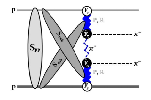
Figure 1: Amplitude of the process of double pion LM CEDP $p+p\to p+\pi^{+}+\pi^{-}+p$ in the KMR approach CEDPw1 -CEDPw3 . The central part of the diagram is the Born amplitude (with Pomeron and two reggeons). A reggeized off-shell pion propagator is shown as a dashed zigzag line. Proton–proton rescattering is depicted as the $S_{pp}$-blob, and “enhanced” corrections are also shown as the $S_{enh}$-blob. The off-shell pion form factor is presented as a black circle.

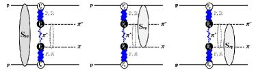
Figure 2: Amplitude of the process of double pion LM CEDP $p+p\to p+\pi^{+}+\pi^{-}+p$ in the approach CEDPw4 -CEDPw6 . The central part of the diagram is the Born amplitude (with Pomeron and two reggeons). A mixture of reggeized and bare off-shell pion propagators is shown as a dashed zigzag line plus dashed straight line. Proton–proton rescattering is depicted as the $S_{pp}$-blob, and pion–proton rescattering corrections are also shown as $S_{\pi p}$-blobs. The off-shell pion form factor is presented as a black circle.

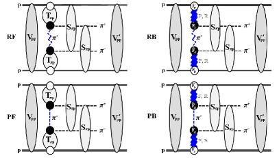
Figure 3: Amplitude of the process of double pion LM CEDP $p+p\to p+\pi^{+}+\pi^{-}+p$ in the Regge-eikonal approach for different cases. PB: central part of the diagram is the Born amplitude (with Pomeron and two reggeons) plus an off-shell bare pion propagator depicted as a dashed straight line. RB: the same as PB, but with the reggeized off-shell pion propagator depicted as a dahshed zigzag line. PF: central part of the diagram contains full eikonalized pion–proton amplitudes plus off-shell bare pion propagator depicted as a dashed straight line. RF: the same as before but with reggeized off-shell pion propagator depicted as a dashed zigzag line. Proton–proton rescatterings in the initial and final states are depicted as $V_{pp}$- and $V^{\prime}_{pp}$-blobs, respectively, and pion–proton rescattering corrections are also shown as $S_{\pi p}$-blobs. The off-shell pion form factor is presented as a black circle.

1 General framework for calculations of LM CEDP

LM CEDP is the first exclusive two to four process which is driven by the Pomeron–Pomeron fusion subprocess. That is why it serves as a basic background for LM CEDP of resonances like $f_{0}(980)$, $f_{2}(1270)$. At the moment, for low central pion–pion masses (less than $\sim 3$ GeV), it is a huge problem to use a perturbative approach, that is why we apply the Regge-eikonal method for all the calculations. For proton–proton and proton–pion elastic amplitudes we use the model of godizovpp , godizovpip , which describes all the available experimental data on elastic scattering.

1.1 Components of the framework

LM CEDP process can be calculated in the following scheme (see Fig. 3):

1. We calculate the primary amplitude of the process, which is depicted as the central part of diagrams in Fig. 3. Here we consider four cases to show that only one of them gives the best description of the data on this process. The case PB represents the Born term (the letter P means that we use the usual “bare” virtual pion propagator $1/(\hat{t}-m_{\pi}^{2})$, and B means the Born term (28) in each shoulder or pion–proton elastic subamplitudes of the central primary amplitude). The expressions of pion–proton elastic subamplitudes can be found in Appendix B.

   The case RB is similar to the previous one, and the letter R (instead of P) means that the bare off-shell pion propagator is replaced by the reggeized one

   $${\cal P}_{\pi}(\hat{s},\hat{t}) = \left(\mathrm{ctg}\frac{\pi\alpha_{\pi}(\hat{t})}{2}-\mathrm{i}\right)\cdot$$ (3)

   $$\cdot \frac{\pi\alpha_{\pi}^{\prime}}{2\phantom{\mbox{\large{I}}^{2}}\!\!\!\!\mathrm{\Gamma}(1+\alpha_{\pi}(\hat{t}))}\left(\frac{\hat{s}}{s_{0}}\right)^{\alpha_{\pi}(\hat{t})},$$

   where $\hat{s}$ is the di-pion mass squared and $\hat{t}$ is the square of the momentum transfer between a Pomeron and a pion in the Pomeron–Pomeron fusion process (see Appendix A for details).

   The cases PF (RF) can be obtained from PB (RB) if we replace the Born pion–proton elastic amplitudes to full eikonalized expressions (which is reflected in the replacement of B to F in the notation for these cases), which could be found in Appendix B.

2. After the calculation of the primary LM CEDP amplitude we have to take into account all possible corrections in proton–proton and proton–pion elastic channels due to the unitarization procedure (the so called “soft survival probability” or “rescattering corrections”), which are depicted as $V_{pp}$, $V^{\prime}_{pp}$ and $S_{\pi p}$ blobs in Fig. 3. For the proton–proton and proton–pion elastic amplitudes we use the model of godizovpp , godizovpip (see Appendix B). A possible final pion–pion interaction is not shown in Fig. 3, since we neglect it in the present calculations. RB and PB cases of Fig. 3 are similar to the one in Fig. 2.

In this article we do not consider the so called “enhanced” corrections CEDPw1 -CEDPw3 , since they give nonleading contributions in our model due to the smallness of the triple Pomeron vertex. Also we have no possible absorptive corrections in the pion–pion final elastic channel, since the central mass is low, and also there is a lack of data on this process to define parameters of the model. Nevertheless we will consider these corrections in further work, as was done by some authors recently pipiespagnol , since they could play significant role for masses less than 1 GeV.

Exact kinematics of the two to four process is outlined in Appendix A.

Here we use the model, presented in Appendix B for example. One can use another one, which has been proved to describe well all the available data on proton–proton and proton–pion elastic processes. But it is difficult to find now more than a couple of models which have more or less predictable power (see godizovmodelsfault for a detailed discussion). That is why we use the model, which has been proved to be good in data fitting, especially in the kinematical region of our interest.

The final expression for the amplitude with proton–proton and pion–proton “rescattering” corrections can be written as

$$M^{U}\left(\{p\}\right)=$$

$$=\int\int\frac{d^{2}\vec{q}}{(2\pi)^{2}}\frac{d^{2}\vec{q}^{\prime}}{(2\pi)^{2}}\frac{d^{2}\vec{q}_{1}}{(2\pi)^{2}}\frac{d^{2}\vec{q}_{2}}{(2\pi)^{2}}V_{pp}(s,q^{2})V_{pp}(s^{\prime},q^{\prime 2})$$

$$\times\;\left[S_{\pi^{-}p}(\tilde{s}_{14},q_{1}^{2})M_{0}\left(\{\tilde{p}\}\right)S_{\pi^{+}p}(\tilde{s}_{23},q_{2}^{2})+(3\leftrightarrow 4)\right]$$ (4)

$$M_{0}\left(\{p\}\right)=\phantom{I^{2^{2^{2}}}}$$

$$=T^{el}_{\pi^{+}p}(s_{13},t_{1}){\cal P}_{\pi}(\hat{s},\hat{t})\left[\hat{F}_{\pi}\left(\hat{t}\right)\right]^{2}T^{el}_{\pi^{-}p}(s_{24},t_{2}),$$ (5)

where the functions are defined in (30)–(34) of Appendix B, and the sets of vectors are

$$\{p\}\equiv\{p_{a},p_{b},p_{1},p_{2},p_{3},p_{4}\},$$ (6)

$$\{\tilde{p}\}\equiv\{p_{a}-q,p_{b}+q;p_{1}+q^{\prime}+q_{1},$$

$$\;\;\;\;\;\;\;\;\;\;\;\;p_{2}-q^{\prime}+q_{2},p_{3}-q_{2},p_{4}-q_{1}\},$$ (7)

and

$$\tilde{s}_{14} = \left(p_{1}+p_{4}+q^{\prime}\right)^{2},\;\tilde{s}_{23}=\left(p_{2}+p_{3}-q^{\prime}\right)^{2},$$ (8)

$$s_{ij} = \left(p_{i}+p_{j}\right)^{2},\;t_{1,2}=\left(p_{a,b}-p_{1,2}\right)^{2},$$ (9)

$$\hat{s} = \left(p_{3}+p_{4}\right)^{2},\;\hat{t}=\left(p_{a}-p_{1}-p_{3}\right)^{2}$$ (10)

The off-shell pion form factor is equal to unity on the mass shell, $\hat{t}=m_{\pi}^{2}$, and taken as exponential

$$\hat{F}_{\pi}=\mathrm{e}^{(\hat{t}-m_{\pi}^{2})/\Lambda_{\pi}^{2}},$$ (11)

where $\Lambda_{\pi}$ is taken from the fits to LM CEDP of two pions at low energies (see next section). In this paper we use only exponential form, but it is possible to use other parametrizations (see CEDPw1 -CEDPw6 ). The xponential form shows more appropriate results in the data fitting.

Other functions are defined in Appendix B. Then we can use Eq. (23) to calculate the differential cross-section of the process.

1.2 Nuances of calculations

In the next section one can see that there are some difficulties in the data fitting, which have also been presented in other work CEDPw4 -CEDPw6 . In this section let us discuss some nuances of calculations, which could change the situation.

We have to pay special attention to the amplitudes, where one or more external particles are off their mass shell. The example of such an amplitude is the pion–proton one $T_{\pi^{+}p}$ ($T_{\pi^{-}p}$), which is the part of the CEDP amplitude (see (4)). For this amplitude in the present paper we use the Regge-eikonal model with the eikonal function in the classical Regge form. The “off-shell” condition for one of the pions is taken into account by an additional phenomenological form factor $\hat{F}_{\pi}(\hat{t})$. But there are at least two other possibilities.

The first one was considered in PetrovOffshell . For the amplitude with one particle off-shell the formula

$$T^{*}(s,b)=\frac{\delta^{*}(s,b)}{\delta(s,b)}T(s,b)=\frac{\delta^{*}(s,b)}{\delta(s,b)}\frac{\mathrm{e}^{2\mathrm{i}\delta(s,b)}-1}{2\mathrm{i}}$$ (12)

was used. In our case

$$\delta(s,b)=\delta_{\pi p}(s,b;m_{\pi}^{2},m_{\pi}^{2},m_{p}^{2},m_{p}^{2}),$$

$$\delta^{*}(s,b)=\delta_{\pi p}^{*}(s,b;\hat{t},m_{\pi}^{2},m_{p}^{2},m_{p}^{2})$$

$$\left.\delta_{\pi p}=\delta^{*}_{\pi p}\right|_{\hat{t}\to m_{\pi}^{2}}.$$ (13)

$\delta_{\pi p}$ is the eikonal function (see (26)). This is similar to the introduction of the additional form factor, but in a more consistent way, which takes into account the unitarity condition.

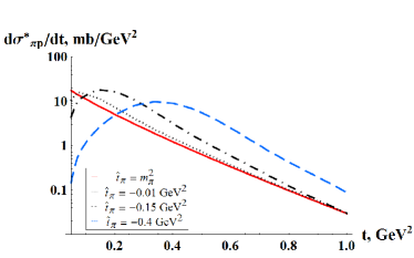
Figure 4: Pion–proton on-shell and off-shell elastic differential cross-section (in the model of conserved meson currents presented in Appendix C) for different pion virtualities $\hat{t}_{\pi}$: $m_{\pi}^{2}$(on-shell),$-0.01$ $\mathrm{GeV}^{2}$,$-0.15$ $\mathrm{GeV}^{2}$,$-0.4$ $\mathrm{GeV}^{2}$ in the covariant approach with conserved currents (50).

The second one arises from the covariant reggeization method, which is considered in Appendix C. For the case of conserved hadronic currents we have the definite structure in the Legendre function (50), which is transformed in a natural way to the case of the off-shell amplitude. But in this case the off-shell amplitude shows a specific behavior at low t values (see Fig. 4 and myCEDP2 for details). As was shown in myCEDP2 , unitarity corrections can mask this behavior. To check this we need to make all the calculations and fitting of the data for the process $p+p\to p+\pi+\pi+p$, but with an amplitude like (50) instead of (33). This will be done in further work on the subject.

In the present calculations we use the linear pion trajectory $0.7(\hat{t}-m_{\pi}^{2})$. The nonlinear case was also verified, and the difference in the final result is not significant.

2 Data from hadron colliders versus results of calculations

Our basic task is to extract the fundamental information on the interaction of hadrons from different cross-sections (“diffractive patterns”):

• from t-distributions we can obtain the size and shape of the interaction region;

• the distribution on the azimuthal angle between the final protons gives the quantum numbers of the produced system (see myCEDP2 ,myWA102 and the references therein);

• from $M_{c}$ (here $M_{c}=M_{\pi\pi}$) dependence and its influence on the t-dependence we can draw some conclusions about the interaction at different space-time scales and the interrelation between them.

The process $p+p\to p+\pi+\pi+p$ is the first “standard candle”, which we can use to estimate other LM CEDP processes, like resonance production myWA102 ,GodizovResonances . In this section we consider the experimental data on the process and its description for different model cases.

2.1 STAR collaboration data versus model cases

In this section the data of the STAR collaboration STARdata1 ,STARdata2 and model curves for different cases of Fig. 3 are presented. In our approach we have only one free parameter, $\Lambda_{\pi}$, that is why all the distributions are depicted for its different values. Also in every case we consider two possibilities: fitting data by formulas with all rescattering corrections (two upper pictures) and also in the approach with proton–proton rescattering only (i.e. fitting the data by formulas without pion–proton interactions in the final state, two lower pictures). We change $\Lambda_{\pi}$ and try to get the best description. As you can see from Figs. 5–8, the best description is given in the RF case for both possibilities (see Fig. 5). Since the final pion–proton interaction can give rather large suppression (about 10–20%, as in Fig. 14), in our further calculations we use the full amplitude as depicted in Fig. 3 for the RF case. The RF case without pion–proton interactions in the final state (with its own values of $\Lambda_{\pi}$ for the best data description) we will show just for cheking of this possibility.

a)

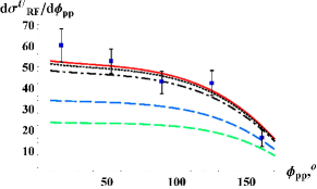
b)

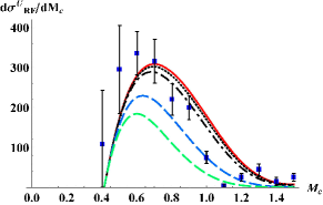
c)

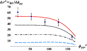
d)

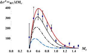
Figure 5: RF case of the model (see Fig. 3). The data on the process $p+p\to p+\pi^{+}+\pi^{-}+p$ at $\sqrt{s}=200$ GeV, $|\eta_{\pi}|<1$, $|\eta_{\pi\pi}|<2$, $p_{T\pi}>0.15$ GeV, $0.005<-t_{1,2}<0.03$ GeV², (STAR collaboration STARdata1 ,STARdata2 ). a, b The result with all p p and $\pi$ p rescattering corrections, c, d show the result, when we try to fit the data by formulas without $\pi$ p rescattering terms. Curves from up to down correspond to different values of the parameter $\Lambda_{\pi}$ in the off-shell pion form factor (11): a, b $\Lambda_{\pi}=5,4,3,1.6,1.2$ GeV, (c),(d) $\Lambda_{\pi}=1.2,1,0.8,0.6$ GeV.

a)

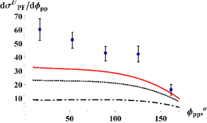
b)

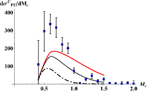
c)

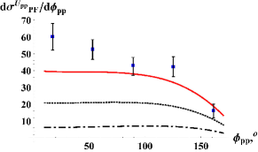
d)

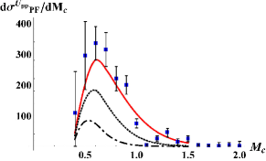
Figure 6: PF case of the model (see Fig. 3). The data on the process $p+p\to p+\pi^{+}+\pi^{-}+p$ at $\sqrt{s}=200$ GeV, $|\eta_{\pi}|<1$, $|\eta_{\pi\pi}|<2$, $p_{T\pi}>0.15$ GeV, $0.005<-t_{1,2}<0.03$ GeV², (STAR collaboration STARdata1 ,STARdata2 ). a, b The result with all p p and $\pi$ p rescattering corrections, c, d show the result when we try to fit the data by formulas without $\pi$ p rescattering terms. Curves from up to down correspond to different values of the parameter $\Lambda_{\pi}$ in the off-shell pion form factor (11): a, b $\Lambda_{\pi}=1.6,1.2,0.8$ GeV, c, d $\Lambda_{\pi}=1,0.8,0.6$ GeV.

a)

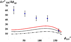
b)

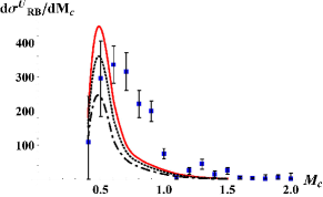
c)

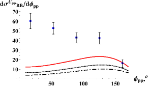
d)

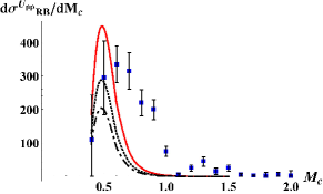
Figure 7: RB case of the model (see Fig. 3). The data on the process $p+p\to p+\pi^{+}+\pi^{-}+p$ at $\sqrt{s}=200$ GeV, $|\eta_{\pi}|<1$, $|\eta_{\pi\pi}|<2$, $p_{T\pi}>0.15$ GeV, $0.005<-t_{1,2}<0.03$ GeV², (STAR collaboration STARdata1 ,STARdata2 ). a, b The result with all p p and $\pi$ p rescattering corrections, c, d show the result when we try to fit the data by formulas without $\pi$ p rescattering terms. Curves from up to down correspond to different values of the parameter $\Lambda_{\pi}$ in the off-shell pion form factor (11): a, b $\Lambda_{\pi}=0.45,0.43,0.4$ GeV, c, d $\Lambda_{\pi}=0.4,0.37,0.35$ GeV.

a)

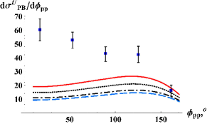
b)

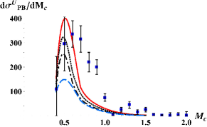
c)

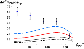
d)

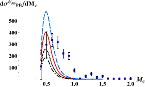
Figure 8: PB case of the model (see Fig. 3). The data on the process $p+p\to p+\pi^{+}+\pi^{-}+p$ at $\sqrt{s}=200$ GeV, $|\eta_{\pi}|<1$, $|\eta_{\pi\pi}|<2$, $p_{T\pi}>0.15$ GeV, $0.005<-t_{1,2}<0.03$ GeV², (STAR collaboration STARdata1 ,STARdata2 ). a, b The result with all p p and $\pi$ p rescattering corrections, c, d show the result when we try to fit the data by formulas without $\pi$ p rescattering terms. Curves from up to down correspond to different values of the parameter $\Lambda_{\pi}$ in the off-shell pion form factor (11): a, b $\Lambda_{\pi}=0.45,0.43,0.41,0.4$ GeV, c, d $\Lambda_{\pi}=0.43,0.4,0.37,0.35$ GeV.

2.2 ISR and CDF data versus RF case of the model

Let us look at the ISR ISRdata1 ,ISRdata2 and CDF CDFdata1 ,CDFdata2 data with parameter $\Lambda_{\pi}$, which we use to describe the data from STAR collaboration. Different cases are depicted on Figs. 9-12.

a)

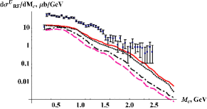
b)

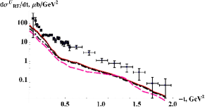
c)

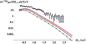
d)

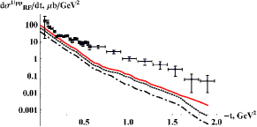
Figure 9: RF case of the model (see Fig. 3) with all rescattering corrections (a, b) and also when we try to fit the data by formulas without final pion–proton rescattering (c, d). The data on the process $p+p\to p+\pi^{+}+\pi^{-}+p$ at $\sqrt{s}=63$ GeV, $|y_{\pi}|<1$, $\xi_{p}>0.9$, (ISR and ABCDHW collaborations ISRdata1 ,ISRdata2 ). Curves from up to down correspond to different values of the parameter $\Lambda_{\pi}$ in the off-shell pion form factor (11): a, b $\Lambda_{\pi}=4,3,1.6,1.2$ GeV, c, d $\Lambda_{\pi}=1.2,1,0.8$ GeV.

a)

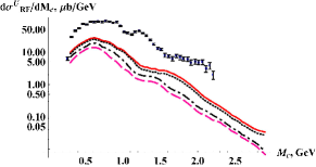
b)

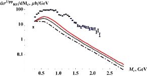
Figure 10: RF case of the model (see Fig. 3) with all rescattering corrections (a) and also when we try to fit the data by formulas without final pion–proton rescattering (b). The data on the process $p+p\to p+\pi^{+}+\pi^{-}+p$ at $\sqrt{s}=62$ GeV, $|y_{\pi}|<1.5$, $\xi_{p}>0.9$, (ISR and ABCDHW collaborations ISRdata1 ,ISRdata2 ). Curves from up to down correspond to different values of the parameter $\Lambda_{\pi}$ in the off-shell pion form factor (11): a $\Lambda_{\pi}=4,3,1.6,1.2$ GeV, b $\Lambda_{\pi}=1.2,1,0.8$ GeV.

a)

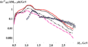
b)

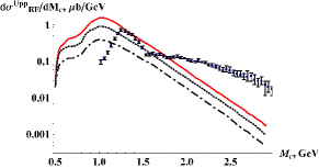
Figure 11: RF case of the model (see Fig. 3) with all rescattering corrections (a) and also when we try to fit the data by formulas without final pion–proton rescattering (b). The data on the process $p+\bar{p}\to p+\pi^{+}+\pi^{-}+\bar{p}$ at $\sqrt{s}=1.96$ TeV, $|\eta_{\pi}|<1.3$, $|y_{\pi\pi}|<1$, $p_{T,\pi}>0.4$ GeV, (CDF collaboration CDFdata1 ,CDFdata2 ). Curves from up to down correspond to different values of the parameter $\Lambda_{\pi}$ in the off-shell pion form factor (11): a $\Lambda_{\pi}=4,3,1.6,1.2$ GeV, b $\Lambda_{\pi}=1.2,1,0.8$ GeV.

a)

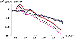
b)

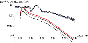
Figure 12: RF case of the model (see Fig. 3) with all rescattering corrections (a) and also when we try to fit the data by formulas without final pion–proton rescattering (b). The data on the process $p+\bar{p}\to p+\pi^{+}+\pi^{-}+\bar{p}$ at $\sqrt{s}=1.96$ TeV, $|\eta_{\pi}|<1.3$, $|y_{\pi\pi}|<1$, $p_{T,\pi}>0.4$ GeV, $p_{T,\pi\pi}>1$ GeV, (CDF collaboration CDFdata1 ,CDFdata2 ). Curves from up to down correspond to different values of the parameter $\Lambda_{\pi}$ in the off-shell pion form factor (11): a $\Lambda_{\pi}=4,3,1.6,1.2$ GeV, b $\Lambda_{\pi}=1.2,1,0.8$ GeV.

We see an underestimation of the ISR data. For these low energies we have to take into account possible corrections to pion–proton amplitudes, since our approach describes data well only for energies greater than $\sim 3$ GeV. In each shoulder ($T_{\pi p}$ amplitude in Fig. 3 RF) the energy can be less than $3$ GeV.

As to the CDF data (Figs. 11, 12), which is overestimated for $M_{\pi\pi}<1.5$ GeV, we can say that there are corrections (destructive interference terms) from resonances to the amplitude, like in Fig. 3 of CEDPw4 ,CEDPw5 and other effects for low $M_{\pi\pi}$, for example, the interference with $\gamma\gamma$ or $\gamma\mathbb{O}$ fusion in the central production process. Also we have to take into account effects related to the irrelevance and possible modifications of the Regge approach (for the virtual pion exchange) in this kinematical region, as was discussed in the introduction.

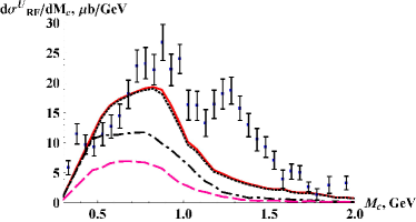
Figure 13: RF case of the model (see Fig. 3) with all rescattering corrections. The data on the process $p+\bar{p}\to p+\pi^{+}+\pi^{-}+\bar{p}$ at $\sqrt{s}=7$ TeV, $|y_{\pi}|<2$, $p_{T,\pi}>0.2$ GeV, (CMS collaboration CMSdata1 ,CMSdata2 ). Curves from up to down correspond to different values of the parameter $\Lambda_{\pi}$ in the off-shell pion form factor (11): $\Lambda_{\pi}=4,3,1.6,1.2$ GeV.

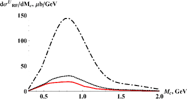
Figure 14: RF case of the model (see Fig. 3) for the CMS energy. Curves from up to down correspond to the Born term, the amplitude with proton–proton rescattering corrections only and the one with all the corrections (proton–proton and pion–proton). $\Lambda_{\pi}=3$ GeV.

2.3 CMS data and predictions

In Fig. 13 one can see the recent data from the CMS collaboration and curves of our model. The upper curve, which corresponds to the parameter $\Lambda_{\pi}$, which better fits the STAR data on $\phi_{pp}$ distribution (but gives higher values for $M_{\pi\pi}>1$ GeV as depicted in Fig. 5b), also describes the data of CMS collaboration well (but overestimates the CDF data, as was shown in Figs. 11, 12). The lower curve underestimates the data from STAR, ISR and CMS, but it is close to the CDF data. Interference with resonances and modifications of the model in the region $|\hat{t}|\sim\hat{s}/2\sim 1$ GeV² can change the picture, especially for low $M_{\pi\pi}$, that is why we have to take it into account when fitting the data (Fig. 14).

2.4 Summary

After the experimental data analysis we have several facts:

• In our approach the best description is given by the case RF (Fig. 3). That is why effects from rescattering (unitarity) corrections are very important.

• The result is crucially dependent on the choice of $\Lambda_{\pi}$ in the off-shell pion form factor, i.e. on $\hat{t}$ (virtuality of the pion) dependence.

• If we try to fit the data from STAR STARdata1 ,STARdata2 , we find that the best description gives overestimation of the CDF data CDFdata1 ,CDFdata2 (especially in the region $M_{\pi\pi}<1.5$ GeV) and underestimation of the ISR data ISRdata1 ,ISRdata2 . This is due to effects like the interference with resonance contributions or $\gamma\gamma\to\pi\pi$ and $\gamma\mathbb{O}\to\pi\pi$ processes, effects related to the irrelevance and possible modifications of the Regge approach (for the virtual pion exchange) in this kinematical region, as was discussed in the introduction, corrections to pion–pion scattering at low $M_{\pi\pi}$, and corrections to $T_{\pi p}(s,t)$ for $\sqrt{s}<3$ GeV;

• Predictions for CMS are close to the data, if we use the best fit to the STAR data on $\phi_{pp}$ distribution (see Fig. 5b). We need also an estimate of the interference with resonance terms to see the full picture and draw final conclusions.

3 Pomeron–Pomeron to pion–pion cross-section

Another interesting question, which we can discuss here, concerns the Pomeron–Pomeron cross-section. As was shown in mySD , it is possible to extract the Pomeron–proton cross-section from the data on single (SD) and double (DD) dissociation, and this numerical value appears to be of the order of typical hadron–hadron cross-sections. It was done by the use of covariant reggeization method with conserved spin-J meson currents,which helps to solve the old problem of the very small Pomeron–proton cross-section extracted by otherauthors kaidalov1 -kaidalov2 .

Reggeon–hadron and reggeon–reggeon scattering can be considered as a scattering of all possible real mesons lying on the Regge trajectory of hadrons. Conceptually it is similar to hydrogen–hadron or hydrogen–hydrogen scattering, since hydrogen has the spectrum of the states, and each of them has its own probability to scatter on a hadron or another hydrogen atom. A specific feature is that we deal in this case with “off-shell atoms”. There is some misunderstanding concerning the physical nature of reggeons. Actually, the reggeon is quite a general notion to qualitatively describe a generic quantum composite system. Conceptually a hadronic reggeon differs from the familiar hydrogen atom only by constituent content: electron–proton in the latter case and, say, quark–antiquark in the former. Energy levels of both are given by the corresponding Regge trajectories. So the reggeon is a full fledged composite particle in the same sense as an atom. Certainly the specific properties are different due to different binding forces.

As was shown also in mySD , absorptive corrections play the crucial role in high energy scattering, and make the extraction procedure rather complicated and model dependent. We should propose some appropriate parametrization for Pomeron–hadron cross-section, then we apply unitarization procedure to obtain real SD or DD cross-sections.

It is possible to perform a similar procedure to extract the Pomeron–Pomeron cross-section. In further work we shall consider the extraction of the total Pomeron–Pomeron cross-section. Here we restrict ourselves by the extraction of the Pomeron–Pomeron to pion–pion one. Let us use the parametrization (4) for CEDP di-pion production to fix one parameter $\Lambda_{\pi}$ from the experimental data. After that we can simply estimate the Pomeron–Pomeron to di-pion cross-section (we use the covariant method from Appendix C):

$$\!\!\!\frac{\mathrm{d}\sigma_{J_{1}J_{2}\to\pi\pi}(\hat{s})}{\mathrm{d}\hat{t}}=$$

$$\!\!\!\frac{1}{(2J_{1}+1)(2J_{2}+1)}\frac{1}{16\pi\lambda(\hat{s},t_{1},t_{2})}\left|{\cal P}_{\pi}(\hat{s},\hat{t})\hat{F}_{\pi}(\hat{t})^{2}\right|\times$$

$$\!\!\!\sum_{\lambda_{1},\lambda_{2}}\left|e_{\mu_{1}\ldots\mu_{J_{1}}}^{(\lambda_{1})}(t_{1})e_{\nu_{1}\ldots\nu_{J_{2}}}^{(\lambda_{2})}(t_{2})F^{J_{1}J_{2}\to\pi\pi}_{\mu_{1}\ldots\mu_{J_{1}},\;\nu_{1}\ldots\nu_{J_{2}}}\right|^{2}=$$

$$\!\!\!\frac{1}{(2J_{1}+1)(2J_{2}+1)}\frac{1}{16\pi\lambda(\hat{s},t_{1},t_{2})}\left|{\cal P}_{\pi}(\hat{s},\hat{t})\hat{F}_{\pi}(\hat{t})^{2}\right|\times$$

$$\!\!\!\Pi_{\mu_{1}\ldots\mu_{J_{1}}}^{\mu^{\prime}_{1}\ldots\mu^{\prime}_{J_{1}}}(t_{1})\Pi_{\nu_{1}\ldots\nu_{J_{2}}}^{\nu^{\prime}_{1}\ldots\nu^{\prime}_{J_{2}}}(t_{2})W^{\mu_{1}\ldots\mu_{J_{1}},\;\nu_{1}\ldots\nu_{J_{2}}}_{\mu^{\prime}_{1}\ldots\mu^{\prime}_{J_{1}},\;\nu^{\prime}_{1}\ldots\nu^{\prime}_{J_{2}}}=$$

$$\!\!\!\!\!\frac{\left|{\cal P}_{\pi}(\hat{s},\hat{t})\hat{F}_{\pi}(\hat{t})^{2}g_{J_{1}}^{\pi}(t_{1})g_{J_{2}}^{\pi}(t_{2})\right|^{2}\!\!\prod_{i=1}^{2}\frac{2^{J_{i}-1}(J_{i}-1)!J_{i}!}{(2J_{i}-1)!}}{(2J_{1}+1)(2J_{2}+1)\cdot 16\pi\lambda(\hat{s},t_{1},t_{2})}\times$$

$$\times{\cal F}_{J_{1}}(t_{1},\hat{t}){\cal F}_{J_{2}}(t_{2},\hat{t}).$$ (14)

Here $\Pi^{\mu^{\prime}_{1}\ldots}_{\mu_{1}\ldots}=\sum_{\lambda}e^{(\lambda)}_{\mu^{\prime}_{1}\ldots}e^{*(\lambda)}_{\mu_{1}\ldots}$ is the structure in the propagator like (53), $e^{(\lambda)}_{\mu_{1}\ldots}$ are polarization tensors,$F^{J_{1}J_{2}\to\pi\pi}_{\mu_{1}\ldots}$ is the Pomeron–Pomeron amplitude and $W^{\mu_{1}...}_{\mu^{\prime}_{1}\ldots}$ is the hadronic tensor for this process made of Pomeron–pion–pion vertices $T_{\mu_{1}\ldots}(p,\Delta)$, where $g^{\pi}_{J}(t)$$=F_{J}(t)/(m_{\pi}^{2}-t/4)^{J/2}$, $F_{J}$ is the leading form factor from (46). After reggeization we get

$$\frac{\mathrm{d}\sigma_{{\mathbb{P}}{\mathbb{P}}\to\pi\pi}(\hat{s})}{\mathrm{d}\hat{t}}=\prod_{i=1}^{2}\frac{2^{\alpha_{\mathbb{P}}(t_{i})-1}\Gamma(\alpha_{\mathbb{P}}(t_{i}))\Gamma(\alpha_{\mathbb{P}}(t_{i})+1)}{\Gamma(2\alpha_{\mathbb{P}}(t_{i}))}$$

$$\frac{\left|{\cal P}_{\pi}(\hat{s},\hat{t})\hat{F}_{\pi}(\hat{t})^{2}g^{\pi}(t_{1})g^{\pi}(t_{2})\right|^{2}{\cal F}(t_{1},\hat{t}){\cal F}(t_{2},\hat{t})}{(2\alpha_{\mathbb{P}}(t_{1})+1)(2\alpha_{\mathbb{P}}(t_{2})+1)\cdot 16\pi\lambda(\hat{s},t_{1},t_{2})},$$ (15)

$$g^{\pi}(t)=\frac{\beta_{\mathbb{P}}(t)2^{\alpha_{\mathbb{P}}(t)}}{\pi\alpha^{\prime}_{\mathbb{P}}(t)g^{p}(t)},$$ (16)

where all the functions are defined in Appendix B. If we use the approach (16), where all terms like

$$2\sqrt{-t}\lambda^{1/2}(m_{i}^{2},m_{j}^{2},t)$$

in (50) are absorbed into the residue, we have to multiply the result by the additional factor ${\cal F}(t_{1},\hat{t}){\cal F}(t_{2},\hat{t})$, where

$${\cal F}(t,\hat{t})=\left(\frac{m_{\pi}^{2}-\frac{\left(m_{\pi}^{2}-\hat{t}+t\right)^{2}}{4t}}{s_{0}}\right)^{\alpha_{\mathbb{P}}(t)}$$ (17)

for conserved currents, and

$${\cal F}(t,\hat{t})\simeq\left(\frac{m_{\pi}^{2}-\frac{\left(m_{\pi}^{2}-\hat{t}+t\right)^{2}}{4m_{J}^{2}}}{s_{0}}\right)^{\alpha_{\mathbb{P}}(t)}$$ (18)

is the leading term for the case of non-conserved currents (see (53)).

a)

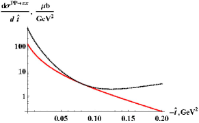
b)

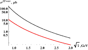
c)

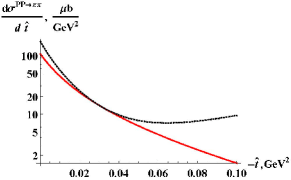
d)

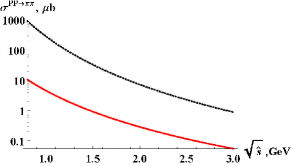
Figure 15: Results of calculations (15)-(17) for Pomeron–Pomeron to pion–pion cross-section for $t_{1,2}=-0.1$ GeV² (a,b) and $t_{1,2}=-0.05$ GeV² (c,d). Two curves present cases of non-conserved (solid) and conserved (dotted) hadronic currents. $\sqrt{\hat{s}}=1.5$ GeV in (a), (c). The parameter of the off-shell form factor is taken $\Lambda_{\pi}=1$ GeV.

Results of calculations (15)–(18) are shown in Fig. 15. In the case of conserved meson currents we obtain Pomeron–Pomeron to pion–pion cross-section $10\div 100$ times higher than in the case of non-conserved currents and with more specific and strong dependence on the Pomeron virtuality. In the old work oldPPtot1 -oldPPtot3 the extracted Pomeron–Pomeron total cross-section was of the order 100 $\mu\mathrm{b}$ at $\sqrt{\hat{s}}<3$ GeV and almost independent on Pomeron’s virtuality. $\sigma_{\mathbb{P}\mathbb{P}\to\pi\pi}$ should be at least less than this number. Our calculations in the same kinematical region give numbers of the order $0.1-5$ $\mu\mathrm{b}$ for non-conserved currents and $0.3-100$ $\mu\mathrm{b}$ for the case of conserved currents. There are strong contributions of other processes (especially production of resonances) in this region, that is why we should have $\sigma_{\mathbb{P}\mathbb{P}\to\pi\pi}\ll\sigma^{tot}_{\mathbb{PP}}$, which is obvious in the case of non-conserved currents where we have both extracted numbers to compare.

In Sect. 2 it is shown that RF and, possibly, PF modes (see Fig. 3 for notations) give an appropriate description of the data, i. e. we have to take into account all rescattering corrections (even in the $T_{\pi p}$ amplitudes). If to use the RB mode, as some other authors do CEDPw1 -CEDPw6 , it is possible to extract the Pomeron–Pomeron cross-section more easily (“almost model independent method”, as was done, for example, for the pion–proton cross-section myLHCf ).

Conclusions

In this paper we have considered the process LM CEDP of di-pions and its description in the framework of the Regge-eikonal approach. Here we summarize all the facts and conclusions:

• After calculations of several cases (see Fig. 3) we can see that the RF case is better suited to describe the data on the process $p+p\to p+\pi^{+}+\pi^{-}+p$.

• When we try to fit the data from STAR collaboration STARdata1 ,STARdata2 with different values of $\Lambda_{\pi}$ (different behavior of the virtual pion form factor), we obtain an underestimation of the ISR data ISRdata1 ,ISRdata2 and an overestimation of the CDF CDFdata1 ,CDFdata2 . Possible explanations are: interference terms with resonances, corrections to $T_{\pi p}(s,t)$ for $\sqrt{s}<3$ GeV, off-shell pion effects, and some other mechanisms in Pomeron–Pomeron to pion–pion process at low $M_{\pi\pi}$.

• We have rather good predictions to the CMS data, when we use the fit to the STAR data on $\phi_{pp}$ distribution depicted on Fig. 5b, but we have to take into account interference with resonances to see the full picture. These main open problems regarding the model parameters are related to interference terms (we have to know all couplings of pions to resonances), which require full spectrum simulation comparisons with data simultaneously in several differential observables. This should be done in further work.

• After estimations of the Pomeron–Pomeron to pion–pion cross-section in the framework of covariant reggeization approach we obtain cross-sections which are (at least in the case of non-conserved Pomeron currents) much lower ($\sim 0.1\div 5\,\mu\mathrm{b}$) than the total Pomeron–Pomeron cross-section, estimated by other authors oldPPtot1 -oldPPtot3 ($\sim 100-300\,\mu\mathrm{b}$), which shows strong contributions from other processes (especially from resonance production). For the case of conserved currents we need re-evaluate old results oldPPtot1 -oldPPtot3 in the same approach.

In further work we will take into account possible modifications of the model (amplitudes for resonances in LM CEDP and their interference with di-pion one, pion–pion cross-section, additional off-shell effects in subamplitudes and so on) for the best description of the data. This model will be implemented to the Monte-Carlo event generator ExDiff ExDiffmanual . It is possible to calculate LM CEDP for other di-hadron final states ($p\bar{p}$ for “Odderon” hunting, $K^{+}K^{-}$, $\eta\eta^{\prime}$ and so on), which are also very informative for our understanding of diffractive mechanisms in strong interactions.

Appendix A. Kinematics of LM CEDP

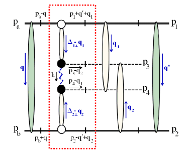
Figure 16: Total amplitude of the process of double pion LM CEDP $\left(p+p\rightarrow p+\pi^{+}+\pi^{-}+p\right)$ with detailed kinematics. Proton–proton rescatterings in the initial and final states are depicted as black blobs, and pion–proton subamplitudes are shown as shaded blobes. All momenta are shown. The basic part of the amplitude, $M_{0}$ (see Eq. (5)), without corrections is circled by a dotted line. Crossed lines are on mass shell. Here $\Delta_{1\perp}=\Delta_{1}-q-q^{\prime}$, $\Delta_{2\perp}=\Delta_{2}+q+q^{\prime}$, $\hat{t}=k^{2}=(\Delta_{1\perp}-q_{1}-p_{3}+q_{2})^{2}$, $\hat{u}=(\Delta_{1\perp}-q_{1}-p_{4})^{2}$, $\hat{s}=(p_{3}+p_{4}-q_{1}-q_{2})^{2}$.

The $2\rightarrow 4$ process $p(p_{a})+p(p_{b})\to p(p_{1})+\pi(p_{3})+\pi(p_{4})+p(p_{2})$ can be described as follows (the notation for any momentum is $k=(k_{0},k_{z};\vec{k})$, $\vec{k}=(k_{x},k_{y})$):

$$p_{a} = \left(\frac{\sqrt{s}}{2},\beta\frac{\sqrt{s}}{2};\vec{0}\right),\;p_{b}=\left(\frac{\sqrt{s}}{2},-\beta\frac{\sqrt{s}}{2};\vec{0}\right),$$

$$p_{1,2} = \left(E_{1,2},p_{1,2z};\vec{p}_{1,2\perp}\right),E_{1,2}=\sqrt{p_{1,2z}^{2}+\vec{p}_{1,2\perp}^{2}+m_{p}^{2}},\;$$

$$p_{3,4} = \left(m_{3,4\perp}\mathrm{ch}\;y_{3,4},m_{3,4\perp}\mathrm{sh}\;y_{3,4};\vec{p}_{3,4\perp}\right)=$$

$$= \left(\sqrt{m_{\pi}^{2}+\vec{p}_{3,4\perp}^{2}\mathrm{ch}^{2}\eta_{3,4}},|\vec{p}_{3,4\perp}|\;\mathrm{sh}\;\eta_{3,4};\vec{p}_{3,4\perp}\right),$$

$$m_{i\perp}^{2} = m_{i}^{2}+\vec{p}_{i\perp}^{2},\;m_{1,2}=m_{p},\;m_{3,4}=m_{\pi},$$

$$\vec{p}_{4\perp} = -\vec{p}_{3\perp}-\vec{p}_{1\perp}-\vec{p}_{2\perp},\;$$

$$\beta = \sqrt{1-\frac{4m_{p}^{2}}{s}},\;s=(p_{a}+p_{b})^{2},\;s^{\prime}=(p_{1}+p_{2})^{2}.$$ (19)

Here the $y_{i}$ ($\eta_{i}$) are the rapidities (pseudorapidities) of the final pions.

The phase space of the process in terms of the above variables is the following

$$\mathrm{d}\mathrm{\Phi}_{2\to 4} = \left(2\pi\right)^{4}\delta^{4}\left(p_{a}+p_{b}-\sum_{i=1}^{4}p_{i}\right)\prod_{i=1}^{4}\frac{\mathrm{d}^{3}p_{i}}{(2\pi)^{3}2E_{i}}=$$

$$= \frac{1}{2^{4}(2\pi)^{8}}\prod_{i=1}^{3}p_{i\perp}\mathrm{d}p_{i\perp}\mathrm{d}\phi_{i}\cdot\mathrm{d}y_{3}\mathrm{d}y_{4}\cdot{\cal J};$$

$${\cal J} = \frac{\mathrm{d}p_{1z}}{E_{1}}\frac{\mathrm{d}p_{2z}}{E_{2}}\delta\left(\sqrt{s}-\sum_{i=1}^{4}E_{i}\right)\delta\left(\sum_{i=1}^{4}p_{iz}\right)=$$ (20)

$$= \frac{1}{\left|\tilde{E}_{2}\tilde{p}_{1z}-\tilde{E}_{1}\tilde{p}_{2z}\right|},$$

where the $p_{i\perp}=\left|\vec{p}_{i}\right|$, $\tilde{p}_{1,2z}$ are the appropriate roots of the system

$$\begin{cases}&A=\sqrt{s}-E_{3}-E_{4}=\sqrt{m_{1\perp}^{2}+p_{1z}^{2}}+\sqrt{m_{2\perp}^{2}+p_{2z}^{2}},\\ &B=-p_{3z}-p_{4z}=p_{1z}+p_{2z},\end{cases}$$ (21)

$$\tilde{p}_{1z} = \frac{B}{2}+\frac{1}{2(A^{2}-B^{2})}\left[B\left(m_{1\perp}^{2}-m_{2\perp}^{2}\right)+A\cdot\lambda_{0}^{1/2}\right],$$

$$\lambda_{0} = \lambda\left(A^{2}-B^{2},m_{1\perp}^{2},m_{2\perp}^{2}\right).$$ (22)

Here $\lambda(x,y,z)=x^{2}+y^{2}+z^{2}-2xy-2xz-2yz$, and then ${\cal J}=\lambda_{0}^{1/2}/2$.

For the differential cross-section we have

$$\frac{\mathrm{d}\sigma_{2\to 4}}{\prod_{i=1}^{3\phantom{I}}\mathrm{d}p_{i\perp}\mathrm{d}\phi_{i}\cdot\mathrm{d}y_{3}\mathrm{d}y_{4}} = \frac{1}{2\beta s}\cdot\frac{\prod_{i=1}^{3}p_{i\perp}}{2^{4}(2\pi)^{8}\cdot\frac{1}{2}\lambda_{0}^{1/2}}\left|T\right|^{2}=$$ (23)

$$= \frac{\prod_{i=1}^{3}p_{i\perp}}{2^{12}\pi^{8}\beta s\lambda_{0}^{1/2}}\left|T\right|^{2}.$$

The pseudorapidity is more convenient experimental variable, and we can use the transform

$$\frac{\mathrm{d}y_{i}}{\mathrm{d}\eta_{i}}=\frac{p_{i\perp}\mathrm{ch}\eta_{i}}{\sqrt{m_{i}^{2}+p_{i\perp}^{2}\mathrm{ch}^{2}\eta_{i}}}$$ (24)

to get the differential cross-section in the pseudorapidities.

For exact calculations of the elastic subprocesses (see Fig. 16) of the type
$a(p_{1})+b(p_{2})\rightarrow c(p_{1}-q_{el})+d(p_{2}+q_{el})$:

$$q_{el} = \left(q_{0},q_{z};\vec{q}\right),$$

$$q_{z} = -\frac{b}{2a}\left(1-\sqrt{1-\frac{4ac}{b^{2}}}\right),$$

$$q_{0} = \frac{A_{0}q_{z}+\vec{p}_{1\perp}\vec{q}+\vec{p}_{2\perp}\vec{q}}{A_{z}},$$

$$a = A_{z}^{2}-A_{0}^{2},\;b=-2\left(A_{z}\cdot{\cal D}+A_{0}\left(\vec{p}_{1\perp}\vec{q}+\vec{p}_{2\perp}\vec{q}\right)\right),$$

$$c = 2A_{z}B_{z}-\left(\vec{p}_{1\perp}\vec{q}+\vec{p}_{2\perp}\vec{q}\right)^{2}+\vec{q}^{2}A_{z}^{2},$$

$$A_{0} = p_{1z}+p_{2z},\;A_{z}=p_{10}+p_{20},$$

$$B_{0} = p_{1z}\cdot\vec{p}_{2\perp}\vec{q}-p_{2z}\cdot\vec{p}_{1\perp}\vec{q},$$

$$B_{z} = p_{10}\cdot\vec{p}_{2\perp}\vec{q}-p_{20}\cdot\vec{p}_{1\perp}\vec{q},$$

$${\cal D} = p_{1z}p_{20}-p_{2z}p_{10},$$ (25)

and $q_{el}^{2}\simeq-\vec{q}^{2}$.

Appendix B. Regge-eikonal model for elastic proton–proton and pion–proton scattering

Here is a short review of the formulas for the Regge-eikonal approach godizovpp , godizovpip , which we use to estimate rescattering corrections in the proton–proton and pion–proton channels.

The amplitudes of elastic proton–proton and pion–proton scattering are expressed in terms of the eikonal functions:

$$T_{pp,\pi p}^{el}(s,b) = \frac{\mathrm{e}^{-2\Omega_{pp,\pi p}^{el}(s,b)}-1}{2\mathrm{i}},$$

$$\Omega_{pp,\pi p}^{el}(s,b) = -\mathrm{i}\,\delta_{pp,\pi p}^{el}(s,b),$$

$$\delta^{el}_{pp,\pi p}(s,b) = \frac{1}{16\pi s}\int_{0}^{\infty}d(-t)J_{0}(b\sqrt{-t})\delta^{el}_{pp,\pi p}(s,t),$$ (26)

$$\delta^{el}_{pp}(s,t)\simeq$$

$$g_{pp\mathbb{P}}(t)^{2}\left(\mathrm{i}+\tan\frac{\pi(\alpha_{\mathbb{P}}(t)-1)}{2})\right)\pi\alpha^{\prime}_{\mathbb{P}}(t)\left(\frac{s}{2s_{0}}\right)^{\alpha_{\mathbb{P}}(t)},$$

$$\alpha_{\mathbb{P}}(t)=1+\frac{\alpha_{\mathbb{P}}(0)-1}{1-\frac{t}{\tau_{a}}}\,,\,g_{pp\mathbb{P}}(t)=\frac{g_{pp\mathbb{P}}(0)}{\left(1-a_{g}t\right)^{2}}.$$ (27)

$$\delta^{el}_{\pi p}(s,t)\simeq$$

$$\left(\mathrm{i}+\tan\frac{\pi(\alpha_{\mathbb{P}}(t)-1)}{2})\right)\beta_{\mathbb{P}}(t)\left(\frac{s}{s_{0}}\right)^{\alpha_{\mathbb{P}}(t)},$$

$$+\left(\mathrm{i}+\tan\frac{\pi(\alpha_{f}(t)-1)}{2})\right)\beta_{f}(t)\left(\frac{s}{s_{0}}\right)^{\alpha_{f}(t)},$$ (28)

$$\alpha_{\mathbb{P}}(t)=1+p_{1}\left[1-p_{2}t\left(\arctan\left(p_{3}-p_{2}t\right)-\frac{\pi}{2}\right)\right],$$

$$\alpha_{f}(t)=\left(\frac{8}{3\pi}\gamma(\sqrt{-t+c_{f}})\right)^{1/2},$$

$$\gamma(\mu)=\frac{4\pi}{11-\frac{2}{3}n_{f}}\left(\frac{1}{\ln\frac{\mu^{2}}{\Lambda^{2}}}+\frac{1}{1-\frac{\mu^{2}}{\Lambda^{2}}}\right),$$

$$\beta_{\mathbb{P}}(t)=B_{\mathbb{P}}\mathrm{e}^{b_{\mathbb{P}}t}(1+d_{1}t+d_{2}t^{2}+d_{3}t^{3}+d_{4}t^{4}),$$

$$\beta_{f}(t)=B_{f}\mathrm{e}^{b_{f}t}.$$ (29)

The parameters can be found in Tables 1 and 2.

Table 1: Parameters for proton–proton elastic scattering amplitude.

Parameter	Value
$\alpha_{\mathbb{P}}(0)-1$	$0.109$
$\tau_{a}$	$0.535$ GeV2
$g_{pp\mathbb{P}}(0)$	$13.8$ GeV
$a_{g}$	$0.23$ GeV-2

Table 2: Parameters for pion–proton elastic scattering amplitude.

Parameter	Value
$B_{\mathbb{P}}$	$26.7$
$b_{\mathbb{P}}$	$2.36$ GeV-2
$d_{1}$	$0.38$ GeV-2
$d_{2}$	$0.3$ GeV-4
$d_{3}$	$-0.078$ GeV-6
$d_{4}$	$0.04$ GeV-8
$B_{f}$	$67$
$b_{f}$	$1.88$ GeV-2

We have

$$V_{pp}(s,q^{2}) = \int d^{2}\vec{b}\,\mathrm{e}^{\mathrm{i}\vec{q}\vec{b}}\sqrt{1+2\mathrm{i}T_{pp}^{el}(s,b)}=$$ (30)

$$= \int d^{2}\vec{b}\,\mathrm{e}^{\mathrm{i}\vec{q}\vec{b}}\mathrm{e}^{-\Omega_{pp}^{el}(s,b)}=$$

$$= (2\pi)^{2}\delta^{2}\left(\vec{q}\right)+2\pi\bar{T}_{pp}(s,q^{2}),$$

$$\bar{T}_{pp}(s,q^{2}) = \int_{0}^{\infty}b\,db\,J_{0}\left(b\sqrt{-q^{2}}\right)\left[\mathrm{e}^{-\Omega_{pp}^{el}(s,b)}-1\right]$$ (31)

$$S_{\pi p}(s,q^{2}) = \int d^{2}\vec{b}\,\mathrm{e}^{\mathrm{i}\vec{q}\vec{b}}\left(1+2\mathrm{i}T_{\pi p}^{el}(s,b)\right)=$$ (32)

$$= \int d^{2}\vec{b}\,\mathrm{e}^{\mathrm{i}\vec{q}\vec{b}}\mathrm{e}^{-2\Omega_{\pi p}^{el}(s,b)}=$$

$$= (2\pi)^{2}\delta^{2}\left(\vec{q}\right)+2\pi\bar{T}_{\pi p}(s,q^{2}),$$

$$\bar{T}_{\pi p}(s,q^{2}) = \int_{0}^{\infty}b\,db\,J_{0}\left(b\sqrt{-q^{2}}\right)\left[\mathrm{e}^{-2\Omega_{\pi p}^{el}(s,b)}-1\right]$$ (33)

Here we take $S_{\pi p}(s,t)=S_{\pi^{+}p}(s,t)=S_{\pi^{-}p}(s,t)$ and

$$T^{el}_{\pi^{+}p}(s,t)=T^{el}_{\pi^{-}p}(s,t)=4\pi s\bar{T}_{\pi p}(s,t)$$ (34)

The approach (28) describes the data on pion–proton scattering better even at low energies, that is why we use it instead of the one presented in godizovpp .

The functions $\bar{T}_{pp}$ and $\bar{T}_{\pi p}$ are convenient for numerical calculations, since the oscillations are not so strong.

Appendix C. Covariant basis and Pomeron–Pomeron to di-pion cross-section

In the classical covariant reggeization, as was considered, for example, in oldcovreg , and in the author’s papers mySD ,myCEDP2 , we have the following structure of the amplitudes. Basic elements of such an approach are the vertex functions $T^{\mu_{1}\ldots\mu_{J}}(p,q)$, where

$$T^{\mu_{1}\dots\mu_{J}}(p,q)=<p-q|I^{\mu_{1}\dots\mu_{J}}|p>,$$ (35)

hadronic tensor

$$W^{\mu_{1}\ldots\mu_{J}\nu_{1}\ldots\nu_{J^{\prime}}}(p,q)=$$

$$\int d^{4}x\;e^{iqx}\left<p|\;I^{\mu_{1}\ldots\mu_{J}}(x)I^{\nu_{1}\ldots\nu_{J^{\prime}}}(0)\;|p\right>\quad{,}$$ (36)

and propagators $\Pi_{\mu_{1}\ldots\mu_{J},\;\nu_{1}\ldots\nu_{J}}(J,t)/(m^{2}(J)-t)$ with the tensor structure $\Pi_{\mu_{1}\ldots\nu_{J}}$ calculated in oldcovreg , for example. $1/(m^{2}(J)-t)$ have the poles at

$$m^{2}(J)-t=0,\;\mbox{i.e.}\;J=\alpha_{{\mathbb{P}}}(t)\;,$$ (37)

after an appropriate analytic continuation of the signatured amplitudes in $J$. We assume that this pole, where $\alpha_{\mathbb{P}}$ is the Pomeron trajectory, gives, by definition, the dominant contribution at high energies after having taken the corresponding residues. At this stage we do not take into account absorptive corrections (unitarization).

$I^{\mu_{1}\dots\mu_{J}}$ is the current operator related to the hadronic spin-$J$ Heisenberg field operator,

$$\left(\square+m_{J}^{2}\right)\Phi^{\mu_{1}\dots\mu_{J}}(x)=I^{\mu_{1}\dots\mu_{J}}(x)\;,$$ (38)

and

$$\partial_{\mu}I^{\mu_{1}\ldots\mu\ldots\mu_{J}}=\partial_{\nu}I^{\nu_{1}\ldots\nu\ldots\nu_{J^{\prime}}}=0\;{;}$$ (39)

$$I^{\mu_{1}\ldots\mu_{J}}=I^{\left(\mu_{1}\ldots\mu_{J}\right)}\;{;}\;I^{\nu_{1}\ldots\nu_{J^{\prime}}}=I^{\left(\nu_{1}\ldots\nu_{J^{\prime}}\right)}\;{;}$$ (40)

$$g_{\mu_{i}\mu_{k}}I^{\mu_{1}\ldots\mu_{i}\ldots\mu_{k}\ldots\mu_{J}}=g_{\nu_{i}\nu_{k}}I^{\nu_{1}\ldots\nu_{i}\ldots\nu_{k}\ldots\nu_{J^{\prime}}}=0.$$ (41)

In momentum space the Rarita-Schwinger conditions (39)–(41) for the vertex are

$$T^{\mu_{1}\dots\mu_{i}\dots\mu_{j}\dots\mu_{J}}=T^{\mu_{1}\dots\mu_{j}\dots\mu_{i}\dots\mu_{J}}$$ (42)

$$q_{\mu_{i}}T^{\mu_{1}\dots\mu_{i}\dots\mu_{J}}=0$$ (43)

$$g_{\mu_{i}\mu_{j}}T^{\mu_{1}\dots\mu_{i}\dots\mu_{j}\dots\mu_{J}}=0,$$ (44)

and the same conditions are imposed on each group of indices in the tensors $W$ and $\Pi$. Let us note (as was done in oldcovreg ), that conditions (42)-(44) are valid only on the mass shell of the spin-J meson. And when we go to the phase space of the scattering region, these conditions could be relevant only for conserved hadronic currents. However, this may well not be the case.

Let us consider both cases. In the case of conserved currents we can define the main transverse structures:

$$G_{\alpha\beta} = g_{\alpha\beta}-\frac{q_{\alpha}q_{\beta}}{q^{2}}\;{;}$$

$$P_{\alpha} = \left(p_{\alpha}-q_{\alpha}\frac{pq}{q^{2}}\right)/\sqrt{m^{2}-(pq)^{2}/q^{2}},\;P^{2}=1,$$

$$K_{\alpha} = \left(k_{\alpha}-q_{\alpha}\frac{kq}{q^{2}}\right)/\sqrt{m^{2}-(kq)^{2}/q^{2}},\;K^{2}=1;$$

$$G_{\alpha\beta}P^{\beta} = P_{\alpha},\;G_{\alpha\beta}K^{\beta}=K_{\alpha},$$

$$g_{\alpha\beta}G^{\alpha\beta} = G_{\alpha\beta}G^{\alpha\beta}=3.$$ (45)

For the vertex functions $T$ we can obtain the following tensor decomposition:

$$T^{(J)}\equiv T^{\mu_{1}\dots\mu_{J_{i}}}(k,q)=$$

$$\phantom{T^{(J)}\equiv}F_{J}(t)\sum_{n=0}^{\left[\frac{J}{2}\right]}\frac{{\mathbb{C}}_{J}^{n}}{{\mathbb{C}}_{J}^{0}}\left(K^{(J-2n)}G^{(n)}\right)\;,$$ (46)

$$\phantom{T^{(J)}\equiv}{\mathbb{C}}_{J}^{n}=\frac{(-1)^{n}(2(J-n))\mbox{!}}{(J-n)\mbox{!}n\mbox{!}(J-2n)\mbox{!}},$$ (47)

where the tensor structures $\left(K^{(J-2n)}G^{(n)}\right)^{\mu_{1}\dots\mu_{J}}$ satisfy only the two conditions (42) and (43) (transverse-symmetric):

$$\left(K^{(J-2n)}G^{(n)}\right)=$$

$$\frac{K^{\;(\mu_{1}}\!\!\cdot_{\cdots}\!\!\cdot K^{\;\mu_{J-2n}}G^{\mu_{J-2n+1}\mu_{J-2n+2}}\!\!\cdot_{\cdots}\!\!\cdot G^{\mu_{J-1}\mu_{J})}}{N_{J}^{n}},$$ (48)

$$N_{J}^{n}=\frac{J\mbox{!}}{2^{n}n\mbox{!}(J-2n)\mbox{!}}.$$ (49)

The coefficients ${\mathbb{C}}_{J}^{n}$ in (46) can be obtained from the condition (44) which leads to the recurrent set of equations (see myCEDP2 ). It was also shown in myCEDP2 that, for elastic scattering of particles with equal masses, which can be obtained by the contraction $T_{\{\mu\}}(p_{a},\Delta)\otimes T_{\{\mu\}}(p_{b},-\Delta)$, we have the usual Regge expression for the amplitude. In the general elastic process $a+b\to c+d$ with unequal masses of particles we can obtain

$$\!\!\!\!\!{\cal M}(s,t)=T^{(J)}_{\{\mu\}}(p_{a},\Delta)\otimes T^{(J)}_{\{\mu\}}(p_{b},-\Delta)=$$

$$\!\!\!\!\!=F^{(1)}_{J}(t)F^{(2)}_{J}(t)2^{J}\times$$

$$\!\!\!\!\!{\cal P}_{J}\left(\frac{(s-m_{a}^{2}-m_{b}^{2}+\frac{(m_{a}^{2}-m_{c}^{2}+t)(m_{b}^{2}-m_{d}^{2}+t)}{2t})(-2t)}{\lambda^{1/2}(m_{b}^{2},m_{d}^{2},t)\;\lambda^{1/2}(m_{a}^{2},m_{c}^{2},t)}\right)$$ (50)

Here the argument of the Legendre function is the t-channel cosine $z_{t}=\cos\theta_{t}$, and

$$\lambda(x,y,z)=x^{2}+y^{2}+z^{2}-2xy-2xz-2yz.$$

In the classical Regge scheme

$$\sum_{J}(2J+1){\cal M}_{J}{\cal P}_{J}(-z_{t})\to\eta_{\mathbb{R}}(t)\beta_{\mathbb{R}}(t)\left(\frac{s}{s_{0}}\right)^{\alpha_{\mathbb{R}}(t)},$$ (51)

where we also have Legendre polynomials.

In the case of non-conserved currents we have no Rarita–Schwinger conditions and could propose only some arguments on behavior of coefficients in tensors

$$T^{(J)}_{\mu_{1}\ldots\mu_{J}}(p,q)=\sum_{n+k\leq J}f_{J}^{n,k}\left\{p^{n}q^{k}g^{\left[(J-n-k)/2\right]}\right\},$$ (52)

$$\Pi_{\mu_{1}\ldots\mu_{J},\;\nu_{1}\ldots\nu_{J}}=Q_{(\mu_{1}\nu_{1}}\ldots Q_{\mu_{J}\nu_{J})}+\mathrm{nonleading},$$ (53)

where

$$p^{n}=p_{\mu_{1}}\ldots p_{\mu_{n}},q^{k}=q_{\mu_{n+1}}\ldots p_{\mu_{n+k}},$$

$$g^{\left[(J-n-k)/2\right]}=g_{\mu_{n+k+1}\mu_{n+k+2}}\ldots g_{\mu_{J-1}\mu_{J}},$$

the tensors $\left\{p^{n}q^{k}g^{\left[(J-n-k)/2\right]}\right\}$ and $Q_{(\mu_{1}(\nu_{1}}\ldots Q_{\mu_{J})\nu_{J})}$ are symmetric on the $\mu_{i}$ and $\nu_{j}$ groups of indices. These arguments are

1. all $f_{J}^{n,k}$ are of the same order of magnitude;

2. the tensor $\Pi$ has the form (53), where

   $$Q_{\mu\nu}=g_{\mu\nu}-q_{\mu}q_{\nu}/m_{J}^{2},$$

   which is equal to $G_{\mu\nu}$ on the mass shell of the spin-J meson, and other terms in (53) give nonleading contributions to the final result.

In this case we have also a simple Regge result like in (51), but without Legendre functions. It is natural to assume that, when the spin-J meson is not far from the mass shell, the structures of vertex and propagator are close to the case of conserved currents.

References

- (1) R. Ryutin, Exclusive double diffractive events: general framework and prospects, Eur. Phys. J. C. 73, 2443 (2013).
- (2) R. Ryutin, Visualizations of exclusive central diffraction, Eur. Phys. J. C. 74, 3162 (2014).
- (3) V.A. Petrov, R.A. Ryutin, Single and double diffractive dissociation and the problem of extraction of the proton–Pomeron cross-section, Int. J. Mod. Phys. A 31, 1650049 (2016).
- (4) J.D. Bjorken, Rapidity gaps and jets as a new-physics signature in very-high-energy hadron–hadron collisions, Phys. Rev. D 47, 101 (1993).
- (5) F. Abe et al. (CDF Collaboration), Observation of rapidity gaps in collisions at 1.8 TeV, Phys. Rev. Lett. 74, 855 (1995).
- (6) M.G. Albrow, A. Rostovtsev, Searching for the Higgs at hadron colliders using the missing mass method, FERMILAB-PUB-00-173 (2000), arXiv: 0009336[hep-ph].
- (7) L.A. Harland-Lang, V.A. Khoze, M.G. Ryskin, Central exclusive production and the Durham model, Int. J. Mod. Phys. A 29, 1446004 (2014).
- (8) L.A. Harland-Lang, V.A. Khoze, M.G. Ryskin, W.J. Stirling, Central exclusive production within the Durham model: a review, Int. J. Mod. Phys. A 29, 1430031 (2014).
- (9) L.A. Harland-Lang, V.A. Khoze, M.G. Ryskin, Modeling exclusive meson pair production at hadron colliders, Eur. Phys. J. C 74, 2848 (2014).
- (10) P. Lebiedowicz, O. Nachtmann, A. Szczurek, Tensor pomeron, vector odderon and diffractive production of meson and baryon pairs in proton–proton collisions, EPJ Web Conf. 206, 06005 (2019).
- (11) P. Lebiedowicz, O. Nachtmann, A. Szczurek, Exclusive diffractive production of continuum and resonances within tensor pomeron approach, EPJ Web Conf. 130, 05011 (2016).
- (12) P. Lebiedowicz, O. Nachtmann, A. Szczurek, Central exclusive diffractive production of via the intermediate state in proton–proton collisions, Phys. Rev. D99, 094034 (2019).
- (13) P. Lebiedowicz, A. Szczurek, Revised model of absorption corrections for the process, Phys. Rev. D 92, 054001 (2015).
- (14) P.D.B. Collins, An Introduction to Regge Theory and High Energy Physics, Cambridge University Press, 1977.
- (15) R. Waldi, K.R. Schubert and K. Winter, Search for glueballs in a pomeron pomeron scattering experiment, Z. Phys. C 18, 301 (1983).
- (16) A. Breakstone et al. (ABCDHW Collaboration), The reaction Pomeron–Pomeron and an unusual production mechanism for the , Z. Phys. C 48, 569 (1990).
- (17) L. Adamczyk, W. Guryn and J. Turnau, Central exclusive production at RHIC, Int. J. Mod. Phys. A 29, 1446010 (2014).
- (18) R. Sikora, Central exclusive production of meson pairs in proton–proton collisions at GeV in the STAR experiment at RHIC, talk at Low x Meeting, 1-5 September 2015, Sandomierz, Poland.
- (19) T.A. Aaltonen et al. (CDF Collaboration), Measurement of central exclusive pi+ pi- production in p pbar collisions at and TeV at CDF, Phys. Rev. D 91, 091101 (2015).
- (20) M. Albrow, J. Lewis, M. Zurek, A. Swiech, D. Lontkovskyi, I. Makarenko and J.S. Wilson, the public note called Measurement of Central Exclusive Hadron Pair Production in CDF is available at http://www-cdf.fnal.gov/physics/new/qcd/GXG_14/webpage/ .
- (21) CMS Collaboration, Measurement of exclusive production in proton-proton collisions at TeV, CMS-PAS-FSQ-12-004.
- (22) K. Osterberg, Potential of central exclusive production studies in high runs at the LHC with CMS-TOTEM, Int. J. Mod. Phys. A 29 1446019 (2014).
- (23) A.A. Godizov, Effective transverse radius of nucleon in high-energy elastic diffractive scattering, Eur. Phys. J. C 75, 224 (2015).
- (24) A.A. Godizov, Asymptotic properties of Regge trajectories and elastic pseudoscalar-meson scattering on nucleons at high energies, Yad. Fiz. 71, 1822 (2008).
- (25) J.R. Pelaez, A. Rodas, J. Ruiz De Elvira, Global parameterization of scattering up to 2 GeV, e-Print: arXiv:1907.13162 [hep-ph].
- (26) A.A. Godizov, Current stage of understanding and description of hadronic elastic diffraction, AIP Conf.Proc. 1523, 145 (2013).
- (27) V.A. Petrov, High-energy implications of extended unitarity, IFVE-95-96, IHEP-95-96, talk given at Blois Conference: 20-24 Jun 1995, Blois, France
- (28) V.A. Petrov, R.A. Ryutin, A.E. Sobol and J.-P. Guillaud, Azimuthal angular distributions in EDDE as spin-parity analyser and glueball filter for LHC, JHEP 0506, 007 (2005).
- (29) A.A. Godizov, High-energy central exclusive production of the lightest vacuum resonance related to the soft Pomeron, Phys. Lett. B 787, 188 (2018).
- (30) A.B. Kaidalov and K.A. Ter-Martirosyan, The pomeron–particle total cross-section and diffractive production of showers at very high energies, Nucl. Phys. B 75, 471 (1974).
- (31) A.B. Kaidalov, Diffractive production mechanisms, Phys. Rept. 50, 157 (1979).
- (32) N. Agababyan et al. (EHS/NA22 Collaboration), Pomeron–Pomeron cross-section from inclusive production of a central cluster in quasi-elastic p and p scattering at 250 GeV/c, Z. Phys. C 60, 229 (1993).
- (33) R.A. Buchl and B.P. Nigam, Possible Behavior of Pomeron–Pomeron Total Cross Section, Prog. Theor. Phys. 55, 1879 (1976).
- (34) K.H. Streng, Pomeron–Pomeron collisions at collider energies, Phys. Lett. B 166, 443 (1986).
- (35) C.G. Roldao and A.A. Natale, Photon–photon and Pomeron–Pomeron processes in peripheralHeavy ion collisions, Phys. Rev. C 61, 064907 (2000).
- (36) N. Armesto and M.A. Braun, The Pomeron–Pomeron interactionin the perturbative QCD, Phys. Lett. B 385, 284 (1996).
- (37) R.A. Ryutin, Total pion–proton cross-section from the new LHCf data on leading neutrons spectra, Eur. Phys. J. C 77, 114 (2017); Erratum: Eur. Phys. J. C 77, 843 (2017).
- (38) R.A. Ryutin, ExDiff Monte–Carlo generator for Exclusive Diffraction. Version 2.0. Physics and manual, e-Print: arXiv:1805.08591 [hep-ph]
- (39) R.L. Ingraham, Covariant Propagators and Vertices for Higher Spin Bosons, Prog. Theor. Phys. 51, 249 (1974).