On the Measurement of Sachs Form Factors in Processes
without and with Proton Spin Flip

Abstract

The physical meaning of the decomposition of the Rosenbluth formula into two terms containing only squares of Sachs form factors has been established. A new method has been proposed for their independent measurement in the $e\vec{p}\to e\vec{p}$ elastic process when the initial proton at rest is fully polarized along the direction of motion of the final proton.

Introduction.—The electric ($G_{E}$) and magnetic ($G_{M}$) form factors of the proton, the so-called Sachs form factors, in elastic scattering of the electron on the proton have been experimentally studied since the mid-1950s. In the case of unpolarized electrons and protons, all experimental data on the behavior of the form factors of the proton were obtained using the Rosenbluth formula Rosen for the differential cross section for the $ep\to ep$ elastic scattering in the laboratory reference frame, where the initial proton is at rest. This formula was obtained in the one-photon exchange and zero electron mass approximations and has the form

$$\frac{d\sigma}{d\Omega_{e}}=\frac{\alpha^{2}E_{2}\cos^{2}(\theta_{e}/2)}{4E_{1}^{\,3}\sin^{4}(\theta_{e}/2)}\frac{1}{1+\tau_{p}}\left(G_{E}^{\,2}+\frac{\tau_{p}}{\varepsilon}G_{M}^{\,2}\right).$$ (1)

Here, $\tau_{p}=Q^{2}/4M^{2}$, $Q^{2}=-q^{2}=4E_{1}E_{2}\sin^{2}(\theta_{e}/2)$ is the square of the momentum transferred to the proton and $M$ is the proton mass; $E_{1}$, $E_{2}$, and $\theta_{e}$ are the energies of the initial and final electrons and the angle of scattering of the electron in the laboratory reference frame, respectively; $\alpha=1/137$ is the fine structure constant; and $\varepsilon=[1+2(1+\tau_{p})\tan^{2}(\theta_{e}/2)]^{-1}$ is the degree of the linear polarization of the virtual photon Dombey ; Rekalo74 ; GL97 varying in the region $0\leqslant\varepsilon\leqslant 1$.

It was established with Eq. (1) that the experimental dependence of the Sachs form factors on $Q^{2}$ up to $Q^{2}\approx 6$ GeV² is dipole and the ratio $R\equiv\mu_{p}G_{E}/G_{M}$ is approximately unity, $R\approx 1$, where $\mu_{p}$=2.79 is the magnetic moment of the proton.

Akhiezer and Rekalo Rekalo74 proposed a method for measuring the ratio of the Sachs form factors based on the transfer of polarization from the longitudinally polarized initial electron to the final proton. This method involves the following formula obtained in Rekalo74 for the ratio of form factors $G_{E}$ and $G_{M}$ in terms of the ratio of the degrees of the transverse, $P_{t}$, and longitudinal, $P_{l}$, polarizations of the scattered proton:

$$R\equiv\frac{\mu_{p}\,G_{E}}{G_{M}}=-\frac{P_{t}}{P_{l}}\frac{E_{1}+E_{2}}{2M}\tan\left(\frac{\theta_{e}}{2}\right).$$ (2)

Precision experiments based on Eq.(2) were performed at Jefferson Lab Jones00 ; Gay01 ; Gay02 ; Puckett12 in the range of $0.5\leqslant Q^{2}(\mbox{GeV}^{2})\leqslant 8.5$. It was found that $R$ decreases linearly with increasing $Q^{2}$ in the range of $0.5\leqslant Q^{2}(\mbox{GeV}^{2})\leqslant 5.6$ as

$$R=1-0.13\,(Q^{2}-0.04)\,\approx 1-Q^{2}/8\,,$$ (3)

which indicates that the form factor $G_{E}$ decreases faster than the form factor $G_{M}$.

Subsequent more accurate measurements of the ratio $R$ based on the Akhiezer–Rekalo Puckett12 and Rosenbluth Qattan methods confirmed the existence of discrepancies. The current status of this problem is reviewed ETG15 .

Since the results of the Sachs form factors measurements based on two experimental methods are greatly differed it would be very important to measure them by another independent ways.

Cross section for the $e\vec{p}\to e\vec{p}$ process in the laboratory reference frame.— In this work, we propose a new method for measuring the squares of the Sachs form factors in the $e\vec{p}\to e\vec{p}$ elastic scattering, where $G_{E}^{\,2}$ and $G_{M}^{\,2}$ can be determined independently from each other from direct measurements of cross sections for the process without and with proton spin flip when the initial proton at rest is fully polarized along the direction of motion of the scattered proton. This work is development of our work GKB2008 .

Let $s_{1}$ and $s_{2}$ be the spin 4-vectors of the initial and final protons with 4-momenta $q_{1}$ and $q_{2}$, respectively, in an arbitrary reference frame. The orthogonality ($s_{i}q_{i}=0$) and normalization ($s_{i}^{2}=-1$) conditions unambiguously provide the following expressions for the time ($s_{i0}$) and space ($\mbox{\boldmath$s$}_{i}$) components of these spin 4-vectors $s_{i}=(s_{i0},\mbox{\boldmath$s$}_{i})$ in terms of their 4-velocities $v_{i}=q_{i}/M$, $v_{i}=(v_{i0},\mbox{\boldmath$v$}_{i})$:

$$s_{i}=(s_{i0},\mbox{\boldmath$s$}_{i}),\;s_{i0}=\mbox{\boldmath$v$}_{i}\,\mbox{\boldmath$c$}_{i},\;\mbox{\boldmath$s$}_{i}=\mbox{\boldmath$c$}_{i}+\frac{(\mbox{\boldmath$c$}_{i}\mbox{\boldmath$v$}_{i})\,\mbox{\boldmath$v$}_{i}}{1+v_{i0}}\;,$$ (4)

where $\mbox{\boldmath$c$}_{i}$ ($\mbox{\boldmath$c$}_{i}^{2}=1$) are the unit 3-vectors specifying the directions of spin projections ($i=1,2$).

In the laboratory reference frame, where $q_{1}=(M,\mbox{\boldmath$0$})$ and $q_{2}=(q_{20},\mbox{\boldmath$q$}_{2})$, the directions of the spin projections $\mbox{\boldmath$c$}_{1}$ and $\mbox{\boldmath$c$}_{2}$ are chosen such that they coincide with the direction of motion of the final proton:

$$\mbox{\boldmath$c$}=\mbox{\boldmath$c$}_{1}=\mbox{\boldmath$c$}_{2}=\mbox{\boldmath$n$}_{2}=\mbox{\boldmath$q_{2}$}/|\mbox{\boldmath$q$}_{2}|\,.$$ (5)

Then, the spin 4-vectors $s_{1}$ and $s_{2}$ of the initial and final protons, respectively, in the laboratory reference frame have the form

$$s_{1}=(0,\mbox{\boldmath$n$}_{2})\,,\;s_{2}=(|\mbox{\boldmath$v$}_{2}|,v_{20}\,\mbox{\boldmath$n_{2}$})\,,\,\mbox{\boldmath$n$}_{2}=\mbox{\boldmath$q_{2}$}/|\mbox{\boldmath$q$}_{2}|\,.$$ (6)

The proposed method is based on an expression for the differential cross section for the $e\vec{p}\to e\vec{p}$ scattering in the laboratory reference frame obtained in this work for the case where the initial and final protons are polarized and have the common direction of the spin projections $c$ (5):

$$\frac{d\sigma_{\delta_{1},\delta_{2}}}{d\Omega_{e}} = \frac{\alpha^{2}E_{2}\cos^{2}(\theta_{e}/2)}{4E_{1}^{\,3}\sin^{4}(\theta_{e}/2)}\frac{1}{1+\tau_{p}}$$

$$\times \left(\frac{1+\delta_{1}\delta_{2}}{2}\,G_{E}^{\,2}+\frac{1-\delta_{1}\delta_{2}}{2}\,\frac{\tau_{p}}{\varepsilon}\,G_{M}^{\,2}\right).$$

Here $\delta_{1}$ and $\delta_{2}$ are the doubled spin projections of the initial and final protons on the common direction of the spin projections $c$ (5), meanwhile, $-1\leqslant\delta_{1,2}\leqslant 1$.

Two terms in Eq. (On the Measurement of Sachs Form Factors in Processes without and with Proton Spin Flip) are contributions from transitions without ($\sim G_{E}^{\,2}$) and with ($\sim G_{M}^{\,2}$) proton spin flip in view of the polarization factors

$$\omega_{+}=(1+\delta_{1}\delta_{2})/2,\,\,\omega_{-}=(1-\delta_{1}\delta_{2})/2\,.$$ (8)

Indeed, according to Eq. (On the Measurement of Sachs Form Factors in Processes without and with Proton Spin Flip), only the term containing $G_{E}^{\,2}$ contributes to the cross section for $e\vec{p}$ scattering without proton spin flip ($\delta_{1}=1,\delta_{2}=1$) because $\omega_{+}=1$ and $\omega_{-}=0$ in this case.

Only the term containing $G_{M}^{\,2}$ contributes to the cross section for $e\vec{p}$ scattering with proton spin flip ($\delta_{1}=1$, $\delta_{2}=-1$) because $\omega_{+}=0$ and $\omega_{-}=1$ in this case. Consequently, the cross section the $e\vec{p}\to e\vec{p}$ process given by Eq. (On the Measurement of Sachs Form Factors in Processes without and with Proton Spin Flip) can be represented as the sum of the cross sections for processes without ($\sigma^{\uparrow\uparrow}$) and with ($\sigma^{\downarrow\uparrow}$) proton spin flip:

$$\frac{d\sigma_{\delta_{1},\delta_{2}}}{d\Omega_{e}} = \omega_{+}\sigma^{\uparrow\uparrow}+\omega_{-}\sigma^{\downarrow\uparrow},$$ (9)

$$\sigma^{\uparrow\uparrow} = \sigma_{M}\,G^{2}_{E},\;\;\sigma^{\downarrow\uparrow}=\sigma_{M}\frac{\tau_{p}}{\varepsilon}\,G^{2}_{M}\,,$$ (10)

where

$$\sigma_{M}=\frac{\alpha^{2}E_{2}\cos^{2}(\theta_{e}/2)}{4E_{1}^{\,3}\sin^{4}(\theta_{e}/2)}\frac{1}{1+\tau_{p}}\,.$$

The averaging and summation of Eq. (9) over the polarizations of the initial and final protons give the following representation for the Rosenbluth cross section $\sigma_{R}=d\sigma/d\Omega_{e}$ specified by Eq. (1):

$$\sigma_{R}=\sigma^{\uparrow\uparrow}+\sigma^{\downarrow\uparrow}.$$ (11)

Consequently, the physical meaning of the decomposition of the Rosenbluth formula into two terms containing only $G_{E}^{\,2}$ and $G_{M}^{\,2}$ is the sum of the cross sections for processes without and with proton spin flip when the initial proton at rest is fully polarized along the direction of motion of the final proton. In this case, the electric $G_{E}$ and magnetic $G_{M}$ Sachs form factors determine the contributions of the matrix elements of the proton current for transitions of the proton without and with spin flip.

The validity of this treatment can be easily demonstrated as follows. The Rosenbluth formula (1) for unpolarized particles can be considered (see Eq. (31)) as the sum of cross sections for processes without and with spin flip of the initial proton, which should be fully polarized along a certain direction determined by the kinematics of the process. In the laboratory reference frame, the only separated direction is the direction of motion of the scattered proton, and other separated directions are absent.

It is usually stated in the modern literature, in particular, in textbooks on the physics of elementary particles (see XM ), that the Sachs form factors are simply convenient because they allow the representation of the Rosenbluth formula in the simple and compact form of the sum of two terms containing only $G^{\,2}_{E}$ and $G^{\,2}_{M}$. These formal reasons for advantages of the Sachs form factors are included, in particular, in known monographs AB ; BLP , are not criticized, and are reproduced until now, e.g., in dissertation Paket2015 .

Diagonal spin basis.—In the general case of the system of two particles with different momenta $q_{1}=(q_{10},\mbox{\boldmath$q_{1}$})$ (before interaction) and $q_{2}=(q_{20},\mbox{\boldmath$q_{2}$})$ (after interaction), the possibility of the simultaneous projection of the spins on a single common direction in an arbitrary reference frame is determined by the three-dimensional vector FIF70

$$\mbox{\boldmath$a$}=\mbox{\boldmath$q$}_{2}/q_{20}-\mbox{\boldmath$q$}_{1}/q_{10}\,.$$ (12)

This result was obtained within the vector parameterization of the little Lorentz group $L_{q_{1},q_{2}}$ common for two particles with 4-momenta $q_{1}$ and $q_{2}$ FIF70

$$L_{q_{1}q_{2}}q_{1}=q_{1},\;L_{q_{1}q_{2}}q_{2}=q_{2}\,.$$

In particular, the initial and final protons in the $e\vec{p}\to e\vec{p}$ process can be considered as a system of two particles.

It is noteworthy that the group $L_{q_{1},q_{2}}$ is implemented in a diagonal spin basis Sik84 , where the spin 4-vectors of particles are expressed in terms of their 4-momenta (4-velocities). The term diagonal spin basis is introduced because the three-dimensional vector $a$ given by Eq. (12) is the difference of two vectors and is geometrically the diagonal of a parallelogram.

According to Eq. (12), the common direction of the spin projections in the rest system of the initial proton, where $\mbox{\boldmath$q_{1}$}=0$, coincides with the direction of motion of the final proton: $\mbox{\boldmath$a$}=\mbox{\boldmath$n_{2}$}=\mbox{\boldmath$q_{2}$}/|\mbox{\boldmath$q_{2}$}|$. This confirms that the direction of motion of the final proton in the laboratory reference frame is separate and can be the common direction of the spin projections.

It follows from Eq. (12) that the common direction of the spin projections in the center of mass frame of colliding particles ($\mbox{\boldmath$q$}_{1}+\mbox{\boldmath$q$}_{2}=0$), e.g., in the Breit system of the initial and final protons, where $q_{1}=(q_{0},-\mbox{\boldmath$q$})$, $q_{2}=(q_{0},\mbox{\boldmath$q$})$, and $q=q_{2}-q_{1}=(0,2\mbox{\boldmath$q$})$, as well as in the laboratory reference frame, is the direction of motion of the final proton: $\mbox{\boldmath$a$}=\mbox{\boldmath$n_{2}$}=\mbox{\boldmath$q_{2}$}/|\mbox{\boldmath$q_{2}$}|=\mbox{\boldmath$q$}/|\mbox{\boldmath$q$}|$, coinciding with the direction of the momentum transfer.

In the diagonal spin basis, the spin 4-vectors $s_{1}$ and $s_{2}$ of the initial and final protons (fermions) with 4-velocities $v_{1}$ and $v_{2}$ ($s_{i}v_{i}=0$, $v_{i}^{2}=1$, $s_{i}^{2}=-1$) have the form Sik84

$$s_{1}=-\;\frac{(v_{1}v_{2})v_{1}-v_{2}}{\sqrt{(v_{1}v_{2})^{2}-1}}\;,\;\;s_{2}=\frac{(v_{1}v_{2})v_{2}-v_{1}}{\sqrt{(v_{1}v_{2})^{2}-1}}\,.$$ (13)

The spin 4-vectors given by Eqs. (13) obviously do not change under transformations of the little Lorentz group $L_{q_{1},q_{2}}$ common for particles with 4-momenta $q_{1}$ and $q_{2}$. Therefore, they can be used to describe the spin states of the system of two particles in an arbitrary reference frame by means of spin projections on a single common direction of the 3-vector given by Eq. (12). In particular, the spin 4-vectors $s_{1}$ and $s_{2}$ specified by Eqs. (13) have the form of Eqs. (6) in the laboratory reference frame and correspond to the directions of the spin projections given by Eqs. (5).

The coincidence of the little Lorentz groups for particles with the 4-momenta $q_{1}$ and $q_{2}$ in the diagonal spin basis specified by Eqs. (13) is responsible for a number of remarkable properties of this basis. In particular, in the diagonal spin basis specified by Eqs. (13), the spin projection operators $\sigma_{1}$ and $\sigma_{2}$, as well as the raising and lowering spin operators $\sigma_{1}^{\pm\delta}$ and $\sigma_{2}^{\pm\delta}$, for the initial and final particles coincide with each other GS98 :

$$\sigma=\sigma_{1}=\sigma_{2}=\gamma^{5}\hat{s_{1}}\hat{v_{1}}=\gamma^{5}\hat{s_{2}}\hat{v_{2}}=\gamma^{5}\hat{b}_{0}\hat{b}_{3},$$ (14)

$$\sigma^{\pm\delta}=\sigma_{1}^{\pm\delta}=\sigma_{2}^{\pm\delta}=-1/2\,\gamma^{5}\,\hat{b}_{\pm\delta}\,,$$ (15)

$$\sigma u^{\delta}(q_{i})=\delta u^{\delta}(q_{i}),\sigma^{\pm\delta}u^{\mp\delta}(q_{i})=u^{\pm\delta}(q_{i}).$$ (16)

Here, any 4-vector $\hat{a}$ is $\hat{a}=a_{\mu}\gamma^{\mu}$, $\gamma^{5}$ and $\gamma^{\mu}$ are the Dirac matrices, and $b_{\pm\delta}=b_{1}\pm i\,\delta b_{2}$ are the circular 4-vectors such that $b_{\pm\delta}^{~{}2}=0$, $\delta=\pm 1$. In Eqs. (14) and (15), to construct the spin operators, the following tetrad of orthonormalized 4-vectors $b_{A}$ $(A=0,1,2,3)$ is used:

$$b_{0}=q_{+}/\sqrt{q_{+}^{2}}\;,\;b_{3}=q_{-}/\sqrt{-q_{-}^{2}}\;\;,$$ (17)

$$(b_{1})_{\mu}=\varepsilon_{\mu\nu\kappa\sigma}b_{0}^{\nu}b_{3}^{\kappa}b_{2}^{\sigma},\;(b_{2})_{\mu}=\varepsilon_{\mu\nu\kappa\sigma}q_{1}^{\nu}q_{2}^{\kappa}r^{\sigma}/\rho\,,$$

where $q_{+}=q_{2}+q_{1}$, $q_{-}=q_{2}-q_{1}$, $\varepsilon_{\mu\nu\kappa\sigma}$ is the Levi-Civita tensor ($\varepsilon_{1230}=1$), $r$ is the 4-momentum of a particle involved in the reaction different from $q_{1}$ and $q_{2}$ (e.g., 4-momentum of the initial or final electron in the case of the $e\vec{p}\to e\vec{p}$ process under consideration), and $\rho$ is determined from the normalization conditions $b_{1}^{2}=b_{2}^{2}=b_{3}^{2}=-b_{0}^{2}=-1$. The coincidence of the spin operators in the diagonal spin basis (13) makes it possible to separate in the covariant form the interactions without and with spin flip of particles involved in the reaction and, thereby, to trace the dynamics of the spin interaction.

Calculation of matrix elements of the QED processes in the diagonal spin basis.—The amplitudes of QED processes in the scattering channel have the form

$$M^{\pm\delta,\delta}=\overline{u}^{\pm\delta}(q_{2})Q_{in}u^{\delta}(q_{1})\,,$$ (18)

where $u^{\delta}(q_{i})$=$u^{\delta}(q_{i},s_{i})$ are the bispinors of the initial and final states of fermions normalized as $\overline{u}^{\delta}\,(q_{i})u^{\delta}(q_{i})=2M$, $q_{i}^{2}=M^{2}$ $(i=1,2)$, and $Q_{in}$ is the interaction operator.

The calculation of the matrix elements given by Eq. (18) can be reduced to the calculation of the trace of the product of operators:

$$M^{\pm\delta,\delta}={\mathrm{\rm Tr}}(P_{21}^{\pm\delta,\delta}Q_{in}),$$ (19)

$$P_{21}^{\pm\delta,\delta}=u^{\delta}(q_{1})\overline{u}^{\pm\delta}(q_{2}).$$ (20)

The operators $P_{21}^{\pm\delta,\delta}$ (20) can be determined by several methods GS98 ; Cedrik18 . In the used Bogush–Fedorov approach GS98 , in contrast to, e.g., Cedrik18 , the construction of $P_{21}^{\pm\delta,\delta}$ is reduced to the determination of the operators $T_{21}$ and $T_{12}$ defined as

$$u^{\delta}(q_{2})=T_{21}u^{\delta}(q_{1}),\,u^{\delta}(q_{1})=T_{12}u^{\delta}(q_{2}),$$ (21)

such that $T_{12}=T_{21}^{-1}$, $T_{21}T_{12}=1$.

In the diagonal spin basis (13), the operators $T_{21}$ and $T_{12}$ coincide with each other GS98 :

$$T_{21}=T_{12}=\hat{b}_{0}\,.$$

As a result, the operator $P_{21}^{\delta,\delta}$ in Eqs. (20) is given by the formula

$$P_{21}^{\delta,\delta}=u^{\delta}(q_{1})\,\overline{u}^{\delta}(q_{1})\,T_{12}=\tau_{1}^{\delta}\,T_{12}=T_{12}\,\tau_{2}^{\delta}\,,$$ (22)

where $\tau^{\delta}_{i}$=$u^{\delta}(q_{i})\,\overline{u}^{\delta}(q_{i})$ are the projective operators for states of particles with 4-momenta $q_{i}$ and spin 4-vectors $s_{i}$ ($q_{i}s_{i}=0,s_{i}^{2}=-1$, $i=1,2$) given by the formula

$$\tau^{\delta}_{i}=1/2\,(\,\hat{q}_{i}+M)(\,1-\delta\gamma^{5}\hat{s}_{i})\,.$$ (23)

Relations (14) make it possible to represent the operators $\tau^{\delta}_{i}$ (23) in the diagonal spin basis in the form GS98 :

$$\tau^{\delta}_{i}=-1/4\;(\hat{q}_{i}+M)\;\hat{b}_{\delta}\;\hat{b}_{\delta}^{\ast}\;,$$ (24)

where $b_{\delta}^{\ast}=b_{-\delta}=b_{1}-i\delta b_{2},b_{\delta}b_{\delta}^{\ast}=-2,b_{\delta}^{2}=b_{\delta}^{\ast 2}=0$.

The operator $P_{21}^{-\delta,\delta}$ in Eqs. (20) is reduced to the product of the operators $\sigma^{+\delta}$ (15) and $P_{21}^{-\delta,-\delta}$ (22):

$$P_{21}^{-\delta,\delta}=\sigma^{+\delta}P_{21}^{-\delta,-\delta}=\sigma^{+\delta}\tau^{-\delta}_{1}T_{12}\,=\sigma^{+\delta}T_{12}\tau^{-\delta}_{2}.~{}~{}~{}$$ (25)

As a result, the operators $P_{21}^{\pm\delta,\delta}$ in Eqs. (20) can be represented in the compact form GS98

$$P_{21}^{\delta,\delta}=(\hat{q}_{1}+M)\,\hat{b}_{\delta}\,\hat{b}_{0}\;\hat{b}_{\delta}^{\ast}/4\,,$$ (26)

$$P_{21}^{-\delta,\delta}=\delta(\hat{q}_{1}+M)\;\hat{b}_{\delta}\;\hat{b}_{3}/2\,.$$ (27)

These expressions allow the calculation of matrix elements for QED processes in the diagonal spin basis that correspond to transitions without and with spin flip for any interaction operator $Q_{in}$.

The matrix elements (18) of QED processes can be represented in the most general form

$$M(\delta_{1},\delta_{2})\equiv M^{\pm\delta_{2},\delta_{1}}=\overline{u}^{\pm\delta_{2}}(q_{2})Q_{in}u^{\delta_{1}}(q_{1}).$$ (28)

For them hold true the following identities

$$M(\delta_{1},\delta_{2})=\omega_{+}M^{+\delta_{2},\delta_{1}}+\omega_{-}M^{-\delta_{2},\delta_{1}}.$$ (29)

In view of the properties of the polarization factors $\omega_{\pm}$ (8) at $\delta_{1,2}=\pm 1$ ($\omega_{\pm}^{2}=\omega_{\pm}$, $\omega_{\pm}\omega_{\mp}=0$), we have

$$|M(\delta_{1},\delta_{2})|^{2} = \omega_{+}|M^{+\delta_{2},\delta_{1}}|^{2}+\omega_{-}|M^{-\delta_{2},\delta_{1}}|^{2}\,.$$ (30)

In the $e\vec{p}\to e\vec{p}$ under consideration process with unpolarized electrons, all spin correlations in (30), excepting those in $\omega_{\pm}$ , due to parity conservation in the electromagnetic interactions should be absent. This means that $|M^{\pm\delta_{2},\delta_{1}}|^{2}$ are independent of $\delta_{1}$ and $\delta_{2}$, and the average value of the squared modules of matrix elements (28) summed over all polarizations has the form

$$\overline{|M(\delta_{1},\delta_{2})|^{2}}=|M^{\uparrow\uparrow}|^{2}+|M^{\downarrow\uparrow}|^{2}.$$ (31)

Cross section for the $e\vec{p}\to e\vec{p}$ process in an arbitrary reference frame.—In the one-photon exchange approximation, the matrix element of the elastic process

$$e(p_{1})+p(q_{1},s_{1})\to e(p_{2})+p(q_{2},s_{2})$$ (32)

is the product of the electron and proton currents

$$M_{ep\to ep}=4\pi\alpha T/q^{2}\,,$$ (33)

$$T\equiv T^{\pm\delta,\delta}=(J_{e})^{\mu}(J^{\pm\delta,\delta}_{p})_{\mu}.$$ (34)

The currents $(J_{e})^{\mu}$ and $(J^{\pm\delta,\delta}_{p})_{\mu}$ have the form

$$(J_{e})^{\mu} = \overline{u}(p_{2})\gamma^{\mu}u(p_{1})\,,$$ (35)

$$(J^{\pm\delta,\delta}_{p})_{\mu} = \overline{u}^{\pm\delta}(q_{2})\Gamma_{\mu}(q^{2})u^{\delta}(q_{1})\,,$$ (36)

$$\Gamma_{\mu}(q^{2}) = F_{1}\gamma_{\mu}+\frac{F_{2}}{4M}(\;\hat{q}\gamma_{\mu}-\gamma_{\mu}\hat{q}\;)\,,$$ (37)

where $u(p_{i})$ and $u(q_{i})$ are the bispinors of the electron and proton with the 4-momenta $p_{i}$ and $q_{i}$, respectively; $p_{i}^{2}=m^{2}$, $q_{i}^{2}=M^{2}$, $\overline{u}(p_{i})u(p_{i})=2m$, $\overline{u}(q_{i})u(q_{i})=2M$ $(i=1,2)$; $F_{1}$ and $F_{2}$ are the Dirac and Pauli form factors of the proton; $q=q_{2}-q_{1}$ is the 4-momentum transferred to the proton; and $s_{1}$ and $s_{2}$ are the polarization 4-vectors of the initial and final protons, respectively.

The differential cross section for the $e\vec{p}\to e\vec{p}$ process has the form

$$\frac{d\sigma}{d|t|}=\frac{\pi\alpha^{2}}{4I^{2}}\,\frac{|T|^{2}}{q^{4}}\;,$$ (38)

where $I^{2}=(p_{1}q_{1})^{2}-m^{2}M^{2},|t|=Q^{2}=-q^{2}$.

The matrix elements of the proton current (36) calculated by Eqs. (19), (20), (26), and (27) in the diagonal spin basis (13) have the form Sik84

$$(J^{\delta,\delta}_{p})_{\mu}=2M\,G_{E}(b_{0})_{\mu}\,,$$ (39)

$$(J^{-\delta,\delta}_{p})_{\mu}=-2M\,\delta\sqrt{\tau_{p}}\,G_{M}(b_{\delta})_{\mu}\,,$$ (40)

where

$$G_{E}=F_{1}-\tau_{p}\,F_{2}\,,\;G_{M}=F_{1}+F_{2}$$ (41)

are the Sachs form factors, and $\tau_{p}=-q^{2}/4M^{2}$.

Consequently, the matrix elements of the proton current in the diagonal spin basis that correspond to the proton transitions without and with spin flip given by Eqs. (39) and (40) are expressed only in terms of the Sachs form factors $G_{E}$ and $G_{M}$, respectively. It is precisely because of this factorization of $G_{E}$ and $G_{M}$ that Rosenbluth’s formula is decomposed for the sum of two terms containing only $G_{E}^{2}$ and $G_{M}^{2}$, which are responsible for the contributions of the transitions without and with spin flip of the proton, respectively, when the directions of the spin projections of the protons coincide with each other and have the form (12).

With the use of the matrix elements (39) and (40), the calculation of the quantities $|T|^{2}$ determining the cross section (38) for the $e\vec{p}\to e\vec{p}$ process is reduced to the calculation of traces:

$$|T^{+\delta,\delta}|^{2} = 4M^{2}G^{\,2}_{E}\,{\mathrm{\rm Tr}}((\hat{p}_{2}+m)\hat{b}_{0}(\hat{p}_{1}+m)\hat{b}_{0})/2\,,$$ (42)

$$|T^{-\delta,\delta}|^{2} = 4M^{2}\tau_{p}G^{\,2}_{M}{\mathrm{\rm Tr}}((\hat{p}_{2}+m)\hat{b}_{\delta}(\hat{p}_{1}+m)\hat{b}^{\ast}_{\delta})/2.~{}~{}~{}~{}$$ (43)

The simple calculations give

$$|T^{+\delta,\delta}|^{2} = \frac{G^{\,2}_{E}}{1+\tau_{p}}\,Y_{1},\;\;|T^{-\delta,\delta}|^{2}=\frac{\,\tau_{p}\,G^{\,2}_{M}}{1+\tau_{p}}\,Y_{2}\,,$$ (44)

$$Y_{1} = (p_{+}q_{+})^{2}+q_{+}^{2}q_{-}^{2}\,,$$ (45)

$$Y_{2} = (p_{+}q_{+})^{2}-q_{+}^{2}(q_{-}^{2}+4m^{2})\,,$$ (46)

where $p_{+}=p_{1}+p_{2}$, $q_{+}=q_{1}+q_{2}$, and $q_{-}=q_{2}-q_{1}=q$.

First, the quantities $|T^{\pm\delta,\delta}|^{2}$ given by Eqs. (44) are independent of the polarization of protons in agreement with the above discussion. Second, denominators in Eqs. (44) are due to the normalization of the 4-vector $b_{0}$ in Eqs. (17) and to the relation $q_{+}^{2}=4M^{2}(1+\tau_{p})$.

The quantity $|T|^{2}$ determining the cross section (38) for the $e\vec{p}\to e\vec{p}$ process in the diagonal spin basis (13) has the form (see Eq. (30))

$$|T^{\delta_{1},\delta_{2}}|^{2}=\omega_{+}|T^{+\delta,\delta}|^{2}+\omega_{-}|T^{-\delta,\delta}|^{2}\,.$$ (47)

The calculation of the quantity $|T^{\delta_{1},\delta_{2}}|^{2}$ in the diagonal spin basis by standard methods AB ; BLP also gives a result coinciding with Eq. (47).

The resulting differential cross section for the $e\vec{p}\to e\vec{p}$ process in the diagonal spin basis in an arbitrary reference frame has the form

$$\frac{d\sigma_{\delta_{1},\delta_{2}}}{d|t|}=\frac{\pi\alpha^{2}}{4I^{2}(1+\tau_{p})}\left(\omega_{+}G_{E}^{2}Y_{1}+\omega_{-}\tau_{p}\,G_{M}^{2}Y_{2}\right)\frac{1}{q^{4}}.~{}$$ (48)

The multiplication of Eq. (48) with $\delta_{2}=0$ by a factor of 2 gives the following cross section for the $ep\to ep$ process, where all particles are unpolarized, in an arbitrary reference frame:

$$\frac{d\sigma}{d|t|}=\frac{\pi\alpha^{2}}{4I^{2}\,(1+\tau_{p})}\,(\,G_{E}^{2}\;Y_{1}+\tau_{p}\;G_{M}^{2}\;Y_{2}\,)\,\frac{1}{q^{4}}\,.$$ (49)

This expression coincides with Eq. (34.3.3) from AB .

It is convenient to represent the above expressions for $Y_{1}$ and $Y_{2}$ in terms of the Mandelstam variables:

$$s=(p_{1}+q_{1})^{2},\,t=(q_{2}-q_{1})^{2},\,u=(q_{2}-p_{1})^{2}.$$

Inverting the relation, we have

$$p_{+}q_{+}=s-u,\,q_{+}^{2}=4M^{2}-t,\,q_{-}^{2}=t,\,\tau_{p}=-t/4M^{2},$$

whence

$$Y_{1}=(s-u)^{2}+(4M^{2}-t)\,t,\;\;$$ (50)

$$Y_{2}=(s-u)^{2}-(4M^{2}-t)(t+4m^{2})\,.$$ (51)

The quantity $4I^{2}$ in Eq. (38) has the form

$$4I^{2}=(s-(M+m)^{2})(s-(M-m)^{2})=\lambda(s,m^{2},M^{2}),$$

where $\lambda(s,m^{2},M^{2})$ is the Källén function.

It is noteworthy that, if the mass of the electron is neglected, Eq. (48) in the laboratory reference frame has the form of Eq. (On the Measurement of Sachs Form Factors in Processes without and with Proton Spin Flip), and Eq. (49) written in variables $s,t$, and $u$, coincides with Eq. (139.4) from BLP .

The helicity amplitudes of the $e\vec{p}\to e\vec{p}$ process in the Breit system.— Information reported in the literature is sufficient to understand the physical meaning not only the decomposition of the Rosenbluth formula (1) but also of the Sachs form factors. Such an understanding could be based on exercise (8.7) in XM , where the explicit form of the helicity amplitudes of the proton current $J^{\pm\lambda,\lambda}_{p}$ is presented in the Breit system, where $q_{1}=(q_{0},-\mbox{\boldmath$q$})$ and $q_{2}=(q_{0},\mbox{\boldmath$q$})$, i.e., $q=q_{2}-q_{1}=(0,2\mbox{\boldmath$q$})$. The amplitudes presented in XM have the form

$$(J^{-\lambda,\lambda}_{p})_{\mu}=2M\,G_{E}(b_{0})_{\mu},$$ (52)

$$(J^{\lambda,\lambda}_{p})_{\mu}=-2\lambda\,|\mbox{\boldmath$q$}|\,G_{M}(b_{\lambda})_{\mu},$$ (53)

where $M$ is the proton mass, $2|\mbox{\boldmath$q$}|=\sqrt{Q^{2}}$, $Q^{2}=-q^{2}$, $b_{\lambda}$ is the circular 4-vector, $b_{\lambda}=b_{1}+i\lambda b_{2}$, $\lambda=\pm 1$,

$$(b_{0})^{\mu}=(1,0,0,0),(b_{1})^{\mu}=(0,1,0,0),$$ (54)

$$(b_{2})^{\mu}=(0,0,1,0),(b_{3})^{\mu}=(0,0,0,1)\,.$$

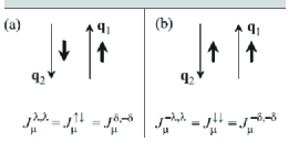
Since the directions of momenta of the initial and final protons in the Breit system are opposite to each other, a transition of the proton with helicity sign conservation is a transition with proton spin flip ($J_{\mu}^{\lambda,\lambda}=J_{\mu}^{\uparrow\downarrow}=J_{\mu}^{\delta,-\delta}$), and a transition of the proton with a change in the helicity sign is a transition without proton spin flip ($J_{\mu}^{-\lambda,\lambda}=J_{\mu}^{\downarrow\downarrow}=J_{\mu}^{-\delta,\,-\delta}$). This is clearly seen in Fig. 1.

Figure 1: Breit system for the initial and final protons, where $\mbox{\boldmath$q$}_{1}+\mbox{\boldmath$q$}_{2}=0$. Long (short) arrows denote the momenta (spins) of protons. Panel (a) corresponds to a transition with helicity conservation ($\lambda_{2}=\lambda_{1}=+1$) at which the proton spin is flipped. Panel (b) corresponds to a transition of a proton with the change in the sign of helicity ($\lambda_{1}=+1,\lambda_{2}=-1$) at which the proton spin is not flipped.

Transitions with helicity conservation are often called transitions without spin flip. The example of the Breit system shows that this statement can be erroneous.

According to the above presentation, the matrix elements given by Eqs. (52) and (53) can be represented in terms of the amplitudes $J_{p}^{\pm\delta,\delta}$ ($\delta=\pm 1$) corresponding to transitions of the proton without and with spin flip for the case where the spins of the initial and final protons are projected on a single common direction coinciding with the direction of motion of the final proton in the Breit system:

$$(J_{p}^{\delta,\delta})_{\mu}=2M\,G_{E}(b_{0})_{\mu},$$ (55)

$$(J_{p}^{-\delta,\delta})_{\mu}=-2\delta M\,\sqrt{\tau_{p}}\,G_{M}(b_{\delta})_{\mu}.$$ (56)

First, the matrix elements specified by Eq. (55) and (56) are more convenient than the helicity amplitudes given by Eqs. (52) and (53), e.g., in the case of passage from the Breit system to the laboratory reference frame, where the notion of helicity is inapplicable for the initial proton. Second, the explicit form of the matrix elements specified by Eq. (55) and (56) coincides with the matrix elements given by Eqs. (39) and (40) in the diagonal spin basis (which are valid in an arbitrary reference frame); amplitudes (55) and (56) are particular cases of matrix elements (39) and (40). To demonstrate this, it is sufficient to verify that the tetrad of 4-vectors (17) is transformed in the Breit system to the tetrad of unit 4-vectors (54). We consider only the 4-vectors $b_{0}$ and $b_{3}$ in Eqs. (17) and (54). Indeed, since the 4-vectors $b_{0}$ and $b_{3}$ in (17) are the sum $q_{+}/\sqrt{q_{+}^{2}}$ and difference $q_{-}/\sqrt{-q_{-}^{2}}$ of 4-momenta of protons normalized to unity, in the Breit system with the third axis along the direction of motion of the final proton, this sum and difference have the form $q_{+}=q_{1}+q_{2}=(2q_{0},0,0,0)$ and $q_{-}=q_{2}-q_{1}=(0,0,0,2|\mbox{\boldmath$q$}|)$. Being normalized, the 4-vectors $b_{0}$ and $b_{3}$ in Eqs. (17) are transformed to the unit 4-vectors $b_{0}=(1,0,0,0)$ and $b_{3}=(0,0,0,1)$ in the Breit system. It can be demonstrated similarly that the 4-vectors $b_{1}$ and $b_{2}$ in Eqs. (17) are transformed to the corresponding 4-vectors of tetrad (54) in the Breit system.

For the inverse transformation of helicity (52) and (53) or diagonal (55) and (56) amplitudes in the Breit system to matrix elements (39) and (40) of the proton current in the diagonal spin basis, the tetrad of vectors (54) appearing in the amplitudes of the proton current $J_{\mu}^{\pm\delta,\delta}$ (55) and (56) should be expressed in terms of the 4-momenta of particles involved in the reaction using the algorithm of construction of the tetrad of 4-vectors (17). In this case, it is not necessary to apply Lorentz transformations to obtain expressions valid in an arbitrary reference frame.

Thus, the example of consideration of matrix elements of the proton current in the Breit system in XM can help to understand the physical meaning of both the decomposition of the Rosenbluth formula and the Sachs form factors. Unfortunately, readers of XM did not notice this assistance.

Since only the time and space components of the 4-vector $J^{-\lambda,\lambda}_{\mu}$ and $J^{\lambda,\lambda}_{\mu}$ in Eqs. (52) and (53) are nonzero, respectively, these 4-vectors are erroneously joined in XM into a single 4-vector, i.e., written in the form

$$(J_{p})_{\mu}=(j_{0},\mbox{\boldmath$j$}),\,j_{0}=(J^{-\lambda,\lambda})_{0},\,\mbox{\boldmath$j$}=\mbox{\boldmath$J$}^{\lambda,\lambda}.$$

The identities in Eqs. (29) allow correcting this error:

$$(J_{p})_{\mu}=\omega_{+}(J_{p}^{+\delta,\delta})_{\mu}+\omega_{-}(J_{p}^{-\delta,\delta})_{\mu}\,,$$ (57)

where $(J_{p}^{\pm\delta,\delta})_{\mu}$ are the matrix elements of the proton current (39) and (40) in the diagonal spin basis.

As a result, for the symmetric parts of the hadron ($H_{\mu\nu}=(J_{p})_{\mu}(J_{p}^{\ast})_{\nu}$) and lepton ($L^{\mu\nu}=(J_{e})^{\mu}(J_{e}^{\ast})^{\nu}$) tensors we have

$$H_{\mu\nu}=\omega_{+}H_{\mu\nu}^{\delta,\delta}+\omega_{-}H_{\mu\nu}^{-\delta,\delta},$$ (58)

$$H_{\mu\nu}^{\delta,\delta}=4M^{2}\,G_{E}^{2}\,\frac{(q_{+})_{\mu}(q_{+})_{\nu}}{q_{+}^{2}}\,,$$ (59)

$$H_{\mu\nu}^{-\delta,\delta}=4M^{2}\tau_{p}\,G_{M}^{2}\,\left(-g_{\mu\nu}+\frac{(q_{+})_{\mu}(q_{+})_{\nu}}{q_{+}^{2}}\right),$$ (60)

$$L^{\mu\nu}=p_{+}^{\mu}p_{+}^{\nu}+q^{2}g^{\mu\nu},$$ (61)

where $g_{\mu\nu}=\rm{diag}(1,-1,-1,-1)$ is the metric tensor in Minkowski space.

Thus, the hadron tensor $H_{\mu\nu}$ (58) in the diagonal spin basis is naturally separated into contributions corresponding to transitions without, Eq. (59), and with, Eq. (60), proton spin flip, which are simultaneously the longitudinal ($H_{\mu\nu}^{\delta,\delta}=H_{\mu\nu}^{L}$) and transverse ($H_{\mu\nu}^{-\delta,\delta}=H_{\mu\nu}^{T}$) contributions, respectively.

The product of the tensors $H_{\mu\nu}$ and $L^{\mu\nu}$ gives Eq. (47) for $|T^{\delta_{1},\delta_{2}}|^{2}$.

Tensor $H_{\mu\nu}$ for unpolarized protons has the form

$$\overline{H}_{\mu\nu}=H_{\mu\nu}^{L}+H_{\mu\nu}^{T}\,.$$ (62)

Conclusions.—The differential cross section for the $e\vec{p}\to e\vec{p}$ process in the diagonal spin basis has been calculated in the Born approximation in an arbitrary reference frame. Expression (On the Measurement of Sachs Form Factors in Processes without and with Proton Spin Flip) obtained for the cross section in the laboratory reference frame can be used to measure the squares of the Sachs form factors, $G_{E}^{\,2}$ and $G_{M}^{\,2}$, in processes without and with spin flip for the case where the initial proton is fully polarized along the direction of motion of the final proton. In the asymptotic limit of large $Q^{2}$ values, where $\tau_{p}\gg 1$, the contribution to cross section (48) comes only from transitions with proton spin flip where helicity is conserved. To understand this, it is sufficient to pass from an arbitrary reference frame to the Breit system and to use Fig. 1. It is noteworthy that the conclusion of spin flip in processes with helicity conservation is valid not only for protons but also for point electrons at $\tau_{e}\gg 1$.