[type=editor, orcid=0000-0002-3311-2100] \creditConceptualization, Methodology, Software, Data Curation, Visualization, Writing - Original Draft
Conceptualization, Methodology, Software, Data Curation, Writing - Review & Editing
Conceptualization, Supervision, Writing - Review & Editing
Conceptualization, Supervision, Writing - Review & Editing
Conceptualization, Supervision
Conceptualization, Supervision, Writing - Review & Editing
Conceptualization, Methodology, Supervision, Writing - Review & Editing \cormark[1] \cortext[cor1]Corresponding author
Backpropagation Algorithms and Reservoir Computing in Recurrent Neural Networks for the Forecasting of Complex Spatiotemporal Dynamics
Abstract
We examine the efficiency of Recurrent Neural Networks in forecasting the spatiotemporal dynamics of high dimensional and reduced order complex systems using Reservoir Computing (RC) and Backpropagation through time (BPTT) for gated network architectures. We highlight advantages and limitations of each method and discuss their implementation for parallel computing architectures. We quantify the relative prediction accuracy of these algorithms for the long-term forecasting of chaotic systems using as benchmarks the Lorenz-96 and the Kuramoto-Sivashinsky (KS) equations. We find that, when the full state dynamics are available for training, RC outperforms BPTT approaches in terms of predictive performance and in capturing of the long-term statistics, while at the same time requiring much less training time. However, in the case of reduced order data, large scale RC models can be unstable and more likely than the BPTT algorithms to diverge. In contrast, RNNs trained via BPTT show superior forecasting abilities and capture well the dynamics of reduced order systems. Furthermore, the present study quantifies for the first time the Lyapunov Spectrum of the KS equation with BPTT, achieving similar accuracy as RC. This study establishes that RNNs are a potent computational framework for the learning and forecasting of complex spatiotemporal systems.
keywords:
Time-series forecasting \sepRNN, LSTM, GRU \sepReservoir Computing \sepBPTT \sepEcho-state networks \sepUnitary RNNs \sepKuramoto-Sivashinsky \sepcomplex systems1 Introduction
In recent years we have observed significant advances in the field of machine learning (ML) that rely on potent algorithms and their deployment on powerful computing architectures. Some of these advances have been materialized by deploying ML algorithms on dynamic environments such as video games (Ha and Schmidhuber, 2018; Schrittwieser et al., 2019) and simplified physical systems (AI gym) (Brockman et al., 2016; Mnih et al., 2015; Silver et al., 2016). Dynamic environments are often encountered across disciplines ranging from engineering and physics to finance and social sciences. They can serve as bridge for scientists and engineers to advances in machine learning and at the same time they present a fertile ground for the development and testing of advanced ML algorithms (Hassabis et al., 2017). The deployment of advanced machine learning algorithms to complex systems is in its infancy. We believe that it deserves further exploration as it may have far-reaching implications for societal and scientific challenges ranging from weather and climate prediction (Weyn et al., 2019; Gneiting and Raftery, 2005), to energy networks, medicine (Esteva et al., 2017; Kurth et al., 2018), and the dynamics of ocean dynamics and turbulent flows (Aksamit et al., 2019; Sünderhauf et al., 2018; Brunton et al., 2020).
Complex systems are characterized by multiple, interacting spatiotemporal scales that challenge classical numerical methods for their prediction and control. The dynamics of such systems are typically chaotic and difficult to predict, a critical issue in problems such as weather and climate prediction. Recurrent Neural Networks (RNNs), offer a potent method for addressing these challenges. RNNs were developed for processing of sequential data, such as time-series (Hochreiter and Schmidhuber, 1997), speech (Graves and Jaitly, 2014), and language (Dong et al., 2015; Cho et al., 2014). Unlike classical numerical methods that aim at discretizing existing equations of complex systems, RNN models are data driven. RNNs keep track of a hidden state, that encodes information about the history of the system dynamics. Such data-driven models are of great importance in applications to complex systems where equations based on first principles may not exist, or may be expensive to discretize and evaluate, let alone control, in real-time.
Early application of neural networks for modeling and prediction of dynamical systems can be traced to the work of Lapedes et. al. (Lapedes and Farber, 1987), where they demonstrated the efficiency of feedforward artificial neural networks (ANNs) to model deterministic chaos. As an alternative to ANNs, wavelet networks were proposed in (Cao et al., 1995) for chaotic time-series prediction. However, these works have been limited to intrinsically low-order systems, and they have been often deployed in conjunction with dimensionality reduction tools. As shown in this work, RNNs have the potential to overcome these scalability problems and be applied to high-dimensional spatio-temporal dynamics. The works of Takens (Takens, 1981) and Sauer, Yorke and Casdagli (Sauer et al., 1991) showed that the dynamics on a D-dimensional attractor of a dynamical system can be unfolded in a time delayed embedding of dimension greater than 2D. The identification of a useful embedding and the construction of a forecasting model have been the subject of life-long research efforts (Bradley and Kantz, 2015). More recently, in (Lusch et al., 2018), a data-driven method based on the Koopman operator formalism (Koopman, 1931) was proposed, using feed-forward ANNs to identify an embedding space with linear dynamics that is then amenable to theoretical analysis.
There is limited work at the interface of RNNs and nonlinear dynamical systems (Vlachas et al., 2018; Wan et al., 2018; Pathak et al., 2017, 2018a; Lu et al., 2018). Here we examine and compare two of the most prominent nonlinear techniques in the forecasting of dynamical systems, namely RNNs trained with backpropagation and Reservoir Computing (RC). We note that our RC implementation also uses a recurrent neural network, but according to the RC paradigm, it does not train the internal network parameters. We consider the cases of fully observed systems as well as the case of partially observed systems such as reduced order models of real world problems, where typically we do not have access to all the degrees-of-freedom of the dynamical system.
Reservoir Computing (RC) has shown significant success in modeling the full-order space dynamics of high dimensional chaotic systems. This success has sparked the interest of theoretical researchers that proved universal approximation properties of these models (Grigoryeva and Ortega, 2018; Gonon and Ortega, 2019). In (Pathak et al., 2017, 2018b) RC is utilized to build surrogate models for chaotic systems and compute their Lyapunov exponents based solely on data. A scalable approach to high-dimensional systems with local interactions is proposed in (Pathak et al., 2018a). In this case, an ensemble of RC networks is used in parallel. Each ensemble member is forecasting the evolution of a group of modes while all other modes interacting with this group is fed at the input of the network. The model takes advantage of the local interactions in the state-space to decouple the forecasting of each mode group and improve the scalability.
RNNs are architectures designed to capture long-term dependencies in sequential data (Pascanu et al., 2013; Bengio et al., 1994; Hochreiter, 1998; Goodfellow et al., 2016). The potential of RNNs for capturing temporal dynamics in physical systems was explored first using low dimensional RNNs (Elman, 1990) without gates to predict unsteady boundary-layer development, separation, dynamic stall, and dynamic reattachment back in 1997 (Faller and Schreck, 1997). The utility of RNNs was limited by the finding that during the learning process the gradients may vanish or explode. In turn, the recent success of RNNs is largely attributed to a cell architecture termed Long Short-Term Memory (LSTM). LSTMs employ gates that effectively remember and forget information thus alleviating the problem of vanishing gradients (Hochreiter, 1998). In the recent years (Bianchi et al., 2017) RNN architectures have been bench-marked for short-term load forecasting of demand and consumption of resources in a supply network, while in (Laptev et al., 2017) they are utilized for extreme event detection in low dimensional time-series. In (Wan and Sapsis, 2018) LSTM networks are used as surrogates to model the kinematics of spherical particles in fluid flows. In (Vlachas et al., 2018) RNNs with LSTM cells were utilized in conjunction with a mean stochastic model to capture the temporal dependencies and long-term statistics in the reduced order space of a dynamical system and forecast its evolution. The method demonstrated better accuracy and scaling to high-dimensions and longer sequences than Gaussian Processes (GPs). In (Wan et al., 2018) the LSTM is deployed to model the residual dynamics in an imperfect Galerkin-based reduced order model derived from the system equations. RC and LSTM networks are applied in the long-term forecasting of partially observable chaotic chimera states in (Neofotistos et al., 2019), where instead of a completely model-free approach, ground-truth measurements of currently observed states are helping to improve the long-term forecasting capability. RNNs are practical and efficient data-driven approximators of chaotic dynamical systems, due to their (1) universal approximation ability (Schäfer and Zimmermann, 2006; Siegelmann and Sontag, 1995) and (2) ability to capture temporal dependencies and implicitly identify the required embedding for forecasting.
Despite the rich literature on both methods there are limited comparative studies of the two frameworks. The present work aims to fill this gap by examining these two machine learning algorithms on challenging physical problems. We compare the accuracy, performance, and computational efficiency of the two methods on the full-order and reduced-order modeling of two prototype chaotic dynamical systems. We also examine the modeling capabilities of the two approaches for reproducing correct Lyapunov Exponents and frequency spectra. Moreover, we include in the present work some more recent RNN architectures, like Unitary (Arjovsky et al., 2016; Jing et al., 2017) and Gated Recurrent Units (GRUs) (Chung et al., 2014; Cho et al., 2014) that have shown superior performance over LSTMs for a wide variety of language, speech signal and polyphonic music modeling tasks.
We are interested in model-agnostic treatment of chaotic dynamical systems, where the time evolution of the full state or some observable is available, but we do not possess any knowledge about the underlying equations. In the latter case, we examine which method is more suitable for modeling temporal dependencies in the reduced order space (observable) of dynamical systems. Furthermore, we evaluate the efficiency of an ensemble of RNNs in predicting the full state dynamics of a high-dimensional dynamical system in parallel and compare it with that of RC. Finally, we discuss the advantages, implementation aspects (such as RAM requirements and training time) and limitations of each model. We remark that the comparison in terms of time and RAM memory consumption, does not aim to quantify advantages/drawback among models but rather provide information for the end users of the software.
We hope that the present study may open to the ML community a new arena with highly structured and complex environments for developing and testing advanced new algorithms (Hassabis et al., 2017). At the same time it may offer a bridge to the physics community to appreciate and explore the importance of advanced ML algorithms for solving challenging physical problems (Brunton et al., 2020).
The structure of the paper is as follows. Section 2 provides an introduction to the tasks and an outline of the architectures and training methods used in this work. Section 3 introduces the measures used to compare the efficiency of the models. In Section 4 the networks are compared in forecasting reduced order dynamics in the Lorenz-96 system. In Section 5, a parallel architecture leveraging local interactions in the state space is introduced and utilized to forecast the dynamics of the Lorenz-96 system (Lorenz, 1995) and the Kuramoto-Sivashinsky equation (Kuramoto, 1978). In Section 6 the GRU and RC networks are utilized to reproduce the Lyapunov spectrum of the Kuramoto-Sivashinsky equation, while Section 7 concludes the paper.
2 Methods - Sequence Modeling
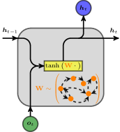
We consider machine learning algorithms for time-series forecasting. The models are trained on time-series of an observable sampled at a fixed rate , , where we eliminate from the notation for simplicity. The models possess an internal high-dimensional hidden state denoted by that enables the encoding of temporal dependencies on past state history. Given the current observable , the output of each model is a forecast for the observable at the next time instant . This forecast is a function of the hidden state. As a consequence, the general functional form of the models is given by
| (1) |
where is the hidden-to-hidden mapping and is the hidden-to-output mapping. All recurrent models analyzed in this work share this common architecture. They differ in the realizations of and and in the way the parameters or weights of these functions are learned from data, i.e., trained, to forecast the dynamics.
2.1 Long Short-Term Memory
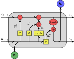
In Elman RNNs (Elman, 1990), the vanishing or exploding gradients problem stems from the fact that the gradient is multiplied repeatedly during back-propagation through time (Werbos, 1988) with a recurrent weight matrix. As a consequence, when the spectral radius of the weight matrix is positive (negative), the gradients are prone to explode (shrink). The LSTM (Hochreiter and Schmidhuber, 1997) was introduced in order to alleviate the vanishing gradient problem of Elman RNNs (Hochreiter, 1998) by leveraging gating mechanisms that allow information to be forgotten. The equations that implicitly define the recurrent mapping of the LSTM are given by
| (2) | ||||||
where , are the gate vector signals (forget, input and output gates), is the observable input at time , is the hidden state, is the cell state, while , , , are weight matrices and biases. The symbol denotes the element-wise product. The activation functions , and are sigmoids. For a more detailed explanation of the LSTM cell architecture refer to (Hochreiter and Schmidhuber, 1997). The dimension of the hidden state (number of hidden units) controls the capacity of the cell to encode history information. The hidden-to-output functional form is given by a linear layer
| (3) |
where . The forget gate bias is initialized to one according to (Jozefowicz et al., 2015) to accelerate training. An illustration of the information flow in a LSTM cell is given in Figure 1(c).
2.2 Gated Recurrent Unit
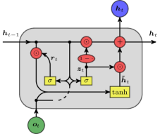
The Gated Recurrent Unit (GRU) (Cho et al., 2014) was proposed as a variation of LSTM utilizing a similar gating mechanism. Even though GRU lacks an output gate and thus has fewer parameters, it achieves comparable performance with LSTM in polyphonic music and speech signal datasets (Chung et al., 2014). The GRU equations are given by
| (4) | ||||
where is the observable at the input at time , is the update gate vector, is the reset gate vector, , is the hidden state, , , are weight matrices and biases. The gating activation is a sigmoid. The output is given by the linear layer:
| (5) |
where . An illustration of the information flow in a GRU cell is given in Figure 1(d).
2.3 Unitary Evolution
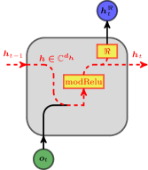
Unitary RNNs (Arjovsky et al., 2016; Jing et al., 2017), similar to LSTMs and GRUs, aim to alleviate the vanishing gradients problem of plain RNNs. Here, instead of employing sophisticated gating mechanisms, the effort is focused on the identification of a re-parametrization of the recurrent weight matrix, such that its spectral radius is a-priori set to one. This is achieved by optimizing the weights on the subspace of complex unitary matrices. The architecture of the Unitary RNN is given by
| (6) | ||||
where is the complex unitary recurrent weight matrix, is the complex input weight matrix, is the complex state vector, denotes the real part of a complex number, is the real output matrix, and the modified ReLU non-linearity is given by
| (7) |
where is the norm of the complex number . The complex unitary matrix is parametrized as a product of a diagonal matrix and multiple rotational matrices. The reparametrization used in this work is the one proposed in (Jing et al., 2017). The complex input weight matrix is initialized with , with real matrices , whose values are drawn from a random uniform distribution according to (Jing et al., 2017). An illustration of the information flow in a Unitary RNN cell is given in Figure 1(b).
In the original paper of (Jing et al., 2017) the architecture was evaluated on a speech spectrum prediction task, a copying memory task and a pixel permuted MNIST task demonstrating superior performance to LSTM either in terms of final testing accuracy or wall-clock training speed.
2.4 Back-Propagation Through Time
Backpropagation dates back to the works of (Dreyfus, 1962; Linnainmaa, 1976; Rumelhart et al., 1986), while its extension to RNNs termed Backpropagation through time (BPTT) was presented in (Werbos, 1988, 1990). A forward pass of the network is required to compute its output and compare it against the label (or target) from the training data based on an error metric (e.g. mean squared loss). Backpropagation amounts to the computation of the partial derivatives of this loss with respect to the network parameters by iteratively applying the chain rule, transversing backwards the network. These derivatives are computed analytically with automatic differentiation. Based on these partial derivatives the network parameters are updated using a first-order optimization method, e.g. stochastic gradient descent.
The power of BBTT lies in the fact that it can be deployed to learn the partial derivatives of the weights of any network architecture with differentiable activation functions, utilizing state-of-the-art automatic differentiation software, while (as the data are processed in small fragments called batches) it scales to large datasets and networks, and can be accelerated by employing Graphics Processing Units (GPUs). These factors made backpropagation the workhorse of state-of-the-art deep learning methods (Goodfellow et al., 2016).
In our study, we utilize BBTT to train the LSTM (Section 2.1), GRU (Section 2.2) and Unitary (Section 2.3) RNNs. There are three key parameters of this training method that can be tuned. The first hyperparameter is the number of forward-pass timesteps performed to accumulate the error for back-propagation. The second parameter is the number of previous time steps for the back-propagation of the gradient . This is also denoted as truncation length, or sequence length. This parameter has to be large enough to capture the temporal dependencies in the data. However, as becomes larger, training becomes much slower, and may lead to vanishing gradients. In the following, we characterize as stateless, models whose hidden state before is hard-coded to zero, i.e., . Stateless models cannot learn dependencies that expand in a time horizon larger that . However, in many practical cases stateless models are widely employed assuming that only short-term temporal dependencies exist. In contrast, stateful models propagate the hidden state between temporally consecutive batches. In our study, we consider only stateful networks.
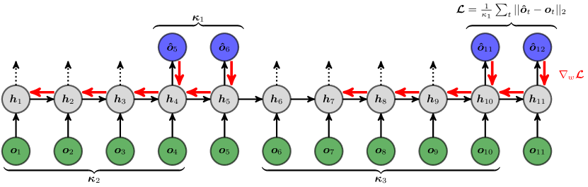
Training stateful networks is challenging because the hidden state has to be available from a previous batch and the network has to be trained to learn temporal dependencies that may span many time-steps in the past. In order to avoid overlap between two subsequent data fragments and compute for the next batch update, the network is teacher-forced for time-steps between two consecutive weight updates. That implies providing ground-truth values at the input and performing forward passing without any back-propagation. This parameter, has an influence on the training speed, as it determines how often the weights are updated. We pick as illustrated in Figure 2, and optimize as a hyperparameter.
The weights of the networks are initialized using the method of Xavier proposed in (Glorot and Bengio, 2010). We utilize a stochastic optimization method with adaptive learning rate called Adam (Kingma and Ba, 2015) to update the weights and biases. We add Zoneout (Krueger et al., 2017) regularization in the recurrent weights and variational dropout (Gal and Ghahramani, 2016) regularization at the output weights (with the same keep probability) to both GRU and LSTM networks to alleviate over-fitting. Furthermore, following (Vlachas et al., 2018) we add Gaussian noise sampled from to the training data, where is the standard deviation of the data. The noise level is tuned. Moreover, we also vary the number of RNN layers by stacking residual layers (He et al., 2016) on top of each other. These deeper architectures may improve forecasting efficiency by learning more informative embedding at the cost of higher computational times.
In order to train the network on a data sequence of time-steps, we pass the whole dataset in pieces (batches) for many iterations (epochs). An epoch is finished when the network has been trained on the whole dataset once. At the beginning of every epoch we sample uniformly integers from the set , and remove them from it. Starting from these indexes we iteratively pass the data through the network till we reach the last (maximum) index in , training it with BBTT. Next, we remove all the intermediate indexes we trained on from . We repeat this process, until , proclaiming the end of the epoch. The batch-size is thus . We experimented with other batch-sizes without significant improvement in performance of the methods used in this work.
As an additional over-fitting counter-measure we use validation-based early stopping, where of the data is used for training and the rest for validation. When the validation error stops decreasing for consecutive epochs, the training round is over. We train the network for rounds decreasing the learning rate geometrically by dividing with a factor of ten at each round to avoid tuning the learning rate of Adam. When all rounds are finished, we pick the model with the lowest validation error among all epochs and rounds.
Preliminary work on tuning the hyperparameters of Adam optimizer apart from the learning rate ( and in the original paper (Kingma and Ba, 2015)), did not lead to important differences on the results. For this reason and due to our limited computational budget, we use the default values proposed in the paper (Kingma and Ba, 2015) ( and ).
Due to the way we train the models (in multiple rounds by decreasing the learning rate when the validation loss saturates and by resetting Adam), we did not notice any important difference on the results. The results were sensitive only when we had one single round and used the learning rate as an additional hyperparameter. Nevertheless, we agree that the hyperparameters of Adam could be included in our studies but in our case this would have exceeded our computing time allocations. We have added a remark on this issue on Section 2.4.
2.5 Reservoir Computing
Reservoir Computing (RC) aims to alleviate the difficulty in learning the recurrent connections of RNNs and reduce their training time (Lukoševičius and Jaeger, 2009; Lukoševičius, 2012). RC relies on randomly selecting the recurrent weights such that the hidden state captures the history of the evolution of the observable and train the hidden-to-output weights. The evolution of the hidden state depends on the random initialization of the recurrent matrix and is driven by the input signal. The hidden state is termed reservoir state to denote the fact that it captures temporal features of the observed state history. This technique has been proposed in the context of Echo-State-Networks (ESNs) (Jaeger and Haas, 2004) and Liquid State Machines with spiking neurons (LSM) (Maass et al., 2002).
In this work, we consider reservoir computers with given by the functional form
| (8) |
where , and . Other choices of RC architectures are possible, including (Larger et al., 2012, 2017; Haynes et al., 2015; Antonik et al., 2017) Following (Jaeger and Haas, 2004), the entries of are uniformly sampled from , where is a hyperparameter. The reservoir matrix has to be selected in a way such that the network satisfies the \sayecho state property. This property requires all of the conditional Lyapunov exponents of the evolution of conditioned on the input (observations ) to be negative so that, for large , the reservoir state does not depend on initial conditions. For this purpose, is set to a large low-degree matrix, scaled appropriately to possess a spectral radius (absolute value of the largest eigenvalue) whose value is a hyperparameter adjusted so that the echo state property holds111Because of the nonlinearity of the tanh function, is not necessarily required for the echo state property to hold true.. The effect of the spectral radius on the predictive performance of RC is analyzed in (Jiang and Lai, 2019). Following (Pathak et al., 2018a) the output coupling is set to
| (9) |
where the augmented hidden state is a dimensional vector such that the th component of is for half of the reservoir nodes and for the other half, enriching the dynamics with the square of the hidden state in half of the nodes. This was empirically shown to improve forecasting efficiency of RCs in the context of dynamical systems (Pathak et al., 2018a). The matrix is trained with regularized least-squares regression with Tikhonov regularization to alleviate overfitting (Tikhonov and Arsenin, 1977; Yan and Su, 2009) following the same recipe as in (Pathak et al., 2018a). The Tikhonov regularization is optimized as a hyperparameter. Moreover, we further regularize the training procedure of RC by adding Gaussian noise in the training data. This was shown to be beneficial for both short-term performance and stabilizing the RC in long-term forecasting. For this reason, we add noise sampled from to the training data, where is the standard deviation of the data and the noise level a tuned hyperparameter.
3 Comparison Metrics
The predictive performance of the models depends on the selection of model hyperparameters. For each model we perform an extensive grid search of optimal hyperparameters, reported in the Appendix. All model evaluations are mapped to a single Nvidia Tesla P100 GPU and are executed on the XC50 compute nodes of the Piz Daint supercomputer at the Swiss national supercomputing centre (CSCS). In the following we quantify the prediction accuracy of the methods in terms of the normalized root mean square error, given by
| (10) |
where is the forecast at a single time-step, is the target value, and is the standard deviation in time of each state component. In Equation 10, the notation denotes the state space average (average of all elements of a vector). To alleviate the dependency on the initial condition, we report the evolution of the NRMSE over time averaged over initial conditions randomly sampled from the attractor.
Perhaps the most basic characterization of chaotic motion is through the concept of Lyapunov exponents (Ott, 2002): Considering two infinitesimally close initial conditions and , their separation on average diverges exponentially in time, , as . Note that the dimensionality of the vector displacement is that of the state space. In general, the Lyapunov exponent depends on the orientation () of the vector displacement . In the limit, the number of possible values of is typically equal to the state space dimensionality. We denote these values and collectively call them the Lyapunov exponent spectrum (LS) of the particular chaotic system. The Lyapunov exponent spectrum will be evaluated in Section 6.
However, we note that a special role is played by , and only , the largest Lyapunov exponent. We refer to the largest Lyapunov exponent as the Maximal Lyapunov exponent (MLE). Chaotic motion of a bounded trajectory is defined by the condition . Importantly, if the orientation of is chosen randomly, the exponential rate at which the orbits separate is with probability one. This is because in order for any of the other exponents () to be realized, must be chosen to lie on a subspace of lower dimensionality than that of the state space; i.e., the orientation of must be chosen in an absolutely precise way never realized by random choice. Hence, the rate at which typical pairs of nearby orbits separate is , and , the \sayLyapunov time, provides a characteristic time scale for judging the quality of predictions based on the observed prediction error growth.
In order to obtain a single metric of the predictive performance of the models we compute the valid prediction time (VPT) in terms of the MLE of the system as
| (11) |
which is the largest time the model forecasts the dynamics with a NRMSE error smaller than normalized with respect to . In the following, we set .
In order to evaluate the efficiency of the methods in capturing the long-term statistics of the dynamical system, we evaluate the mean power spectral density (power spectrum) of the state evolution over all elements of the state (since the state is a vector). The power spectrum of the evolution of is given by dB, where is the complex Fourier spectrum of the state evolution.
4 Forecasting Reduced Order Observable Dynamics in the Lorenz-96
The accurate long-term forecasting of the state of a deterministic chaotic dynamical system is challenging as even a minor initial error can be propagated exponentially in time due to the system dynamics even if the model predictions are perfect. A characteristic time-scale of this propagation is the Maximal Lyapunov Exponent (MLE) of the system as elaborated in Section 3. In practice, we are often interested in forecasting the evolution of an observable (that we can measure and obtain data from), which does not contain the full state information of the system. The observable dynamics are more irregular and challenging to model and forecast because of the additional loss of information.
Classical approaches to forecast the observable dynamics based on Takens seminal work (Takens, 1981), rely on reconstructing the full dynamics in a high-dimensional phase space. The state of the phase space is constructed by stacking delayed versions of the observed state. Assume that the state of the dynamical system is , but we only have access to the less informative observable . The phase space state, i.e., the embedding state, is given by , where the time-lag and the embedding dimension are the embedding parameters. For large enough, and in the case of deterministic nonlinear dynamical chaotic systems, there is generally a one-to-one mapping between a point in the phase space and the full state of the system and vice versa. This implies that the dynamics of the system are deterministically reconstructed in the phase space (Kantz and Schreiber, 1997) and that there exists a phase space forecasting rule , and thus an observable forecasting rule .
The recurrent architectures presented in Section 2 fit to this framework, as the embedding state information can be captured in the high-dimensional hidden state of the networks by processing the observable time series , without having to tune the embedding parameters and .
In the following, we introduce a high-dimensional dynamical system, the Lorenz-96 model and evaluate the efficiency of the methods to forecast the evolution of a reduced order observable of the state of this system. Here the observable is not the full state of the system, and the networks need to capture temporal dependencies to efficiently forecast the dynamics.
4.1 Lorenz-96 Model
The Lorenz-96 model was introduced by Edward Lorenz (Lorenz, 1995) to model the large-scale behavior of the mid-latitude atmosphere. The model describes the time evolution of an atmospheric variable that is discretized spatially over a single latitude circle modelled in the high-dimensional state , and is defined by the equations
| (12) |
for , where we assume periodic boundary conditions , . In the following we consider a grid-size and two different forcing regimes, and .
We solve Equation 12 starting from a random initial condition with a Fourth Order Runge-Kutta scheme and a time-step of . We run the solver up to after ensuring that transient effects are discarded (). The first half samples are used for training and the rest for testing. For the forecasting test in the reduced order space, we construct observables of dimension by performing Singular Value Decomposition (SVD) and keeping the most energetic components. The complete procedure is described in the Appendix. The most energetic modes taken into account in the reduced order observable, explain approximately of the total energy of the system in both .
As a reference timescale that characterizes the chaoticity of the system we use the Lyapunov time, which is the inverse of the MLE, i.e., . The Lyapunov spectrum of the Lorenz-96 system is calculated using a standard technique based on QR decomposition (Abarbanel, 2012). This leads to for and for .
4.2 Results on the Lorenz-96 Model
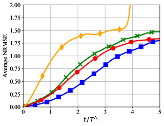
The evolution of the NRMSE of the model with the largest VPT of each architecture for is plotted in Figure 3 for two values of the dimension of the observable , where corresponds to full state information. Note that the observable is given by first transforming the state to its SVD modes and then keeping the most energetic ones. As indicated by the slopes of the curves, models predicting the observable containing full state information () exhibit a slightly slower NRMSE increase compared to models predicting in the reduced order state, as expected.
When the full state of the system is observed, the predictive performance of RC is superior to that of all other models. Unitary networks diverge from the attractor in both reduced order and full space in both forcing regimes . This divergence (inability to reproduce the long-term climate of the dynamics) stems from the iterative propagation of the forecasting error. The issue has been also demonstrated in previous studies in both RC (Pathak et al., 2018b; Lu et al., 2018) and RNNs (Vlachas et al., 2018). This is because the accuracy of the network for long-term climate modeling, depends not only on how well it approximates the dynamics on the attractor locally, but also on how it behaves near the attractor, where we do not have data. As noted in Ref. (Lu et al., 2018), assuming that the network has a full Lyapunov spectrum near the attractor, if any of the Lyapunov exponents that correspond to infinitesimal perturbations transverse to the attractor phase space is positive, then the predictions of the network will eventually diverge from the attractor. Empirically, the divergence effect can also be attributed to insufficient network size (model expressiveness) and training, or attractor regions in the state space that are underrepresented in the training data (poor sampling). Even with a densely sampled attractor, during iterative forecasting in the test data, the model is propagating its own predictions, which might lead to a region near (but not on) the attractor where any positive Lyapunov exponent corresponding to infinitesimal perturbations transverse to the attractor will cause divergence.
In this work, we use samples to densely capture the attractor. Still, RC suffers from the iterative propagation of errors leading to divergence especially in the reduced order forecasting scenario. In order to alleviate the problem, a parallel scheme for RC is proposed in (Pathak et al., 2018b) that enables training of many reservoirs locally forecasting the state. However, this method is limited to systems with local interactions in their state space. In the case we discuss here the observable obtained by singular value decomposition does not fulfill this assumption. In many systems the assumption of local interaction may not hold. GRU and LSTM show superior forecasting performance in the reduced order scenario setting in Lorenz-96 as depicted in Figure 3(a)-Figure 3(c). Especially in the case of , the LSTM and GRU models are able to predict up to Lyapunov times ahead before reaching an NRMSE of , compared to RC and Unitary RNNs that reach this error threshold in Lyapunov time. However, it should be noted that the predictive utility of all models (considering an error threshold of ) is limited to one Lyapunov time when applied to reduced order data and up to two Lyapunov times in the full state.
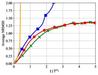
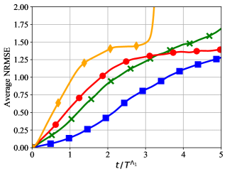
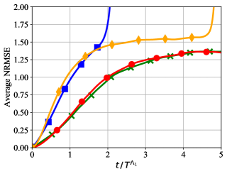
RC ; GRU ; LSTM ; Unit ;
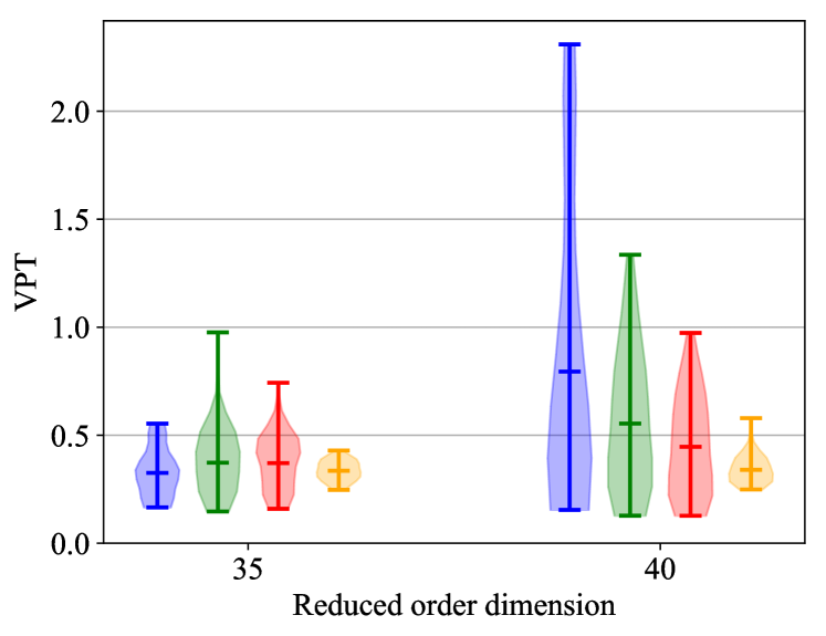
In order to analyze the sensitivity of the VPT to the hyperparameter selection, we present violin plots in Figure 4, showing a smoothed kernel density estimate of the VPT values of all tested hyperparameter sets for and and and . The horizontal markers denote the maximum, average and minimum value. Quantitative results for both are provided on Table 1.
In the full state scenario () and forcing regime , RC shows a remarkable performance with a maximum VPT , while GRU exhibits a max VPT of . The LSTM has a max VPT of , while Unitary RNNs show the lowest forecasting ability with a max VPT of . From the violin plots in Figure 4 we notice that densities are wider at the lower part, corresponding to many models (hyperparameter sets) having much lower VPT than the maximum, emphasizing the importance of tuning the hyperparameters. Similar results are obtained for the forcing regime . One noticeable difference is that the LSTM exhibits a max VPT of which is higher than that of GRU which is . Still, the VPT of RC in the full state scenario is which is the highest among all models.
![[Uncaptioned image]](/html/1910.05266/assets/x10.png)
RC ; GRU ; LSTM ; Unit ;
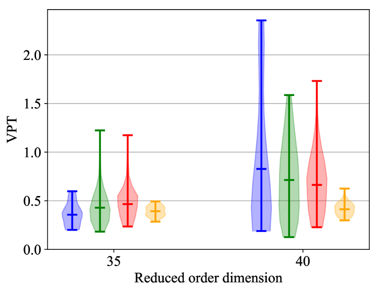
In contrast, in the case of where the models are forecasting on the reduced order space in the forcing regime , GRU is superior to all other models with a maximum VPT compared to LSTM showing a max VPT . LSTM shows inferior performance to GRU which we speculate may be due to insufficient hyperparameter optimization. Observing the results on justifies our claim, as indeed both the GRU and the LSTM show the highest VPT values of and respectively. In both scenarios and , when forecasting the reduced order space , RC shows inferior performance compared to both GRU and LSTM networks with max VPT for and for . Last but not least, we observe that Unitary RNNs show the lowest forecasting ability among all models. This may not be attributed to the expressiveness of Unitary networks, but rather to the difficulty on identifying the right hyperparameters (Greff et al., 2016). Note from the violin plots in Figure 4 that the violin plots in the reduced order state are much thinner at the top compared to the ones in the full state. These results show that hyperparameter sets that achieve a high VPT in the reduced order space are more rare compared to the full state space. This emphasizes that forecasting on the reduced order state is a more difficult task compared to the full state scenario and thus, identification of hyperparameters is more challenging.
In the following, we evaluate the ability of the trained networks to forecast the long-term statistics of the dynamical system. In almost all scenarios and all cases considered in this work, forecasts of Unitary RNN networks fail to remain close to the attractor and diverge. For this reason, we omit the results on these networks.
We quantify the long-term behavior in terms of the power spectrum of the predicted dynamics and its difference with the true spectrum of the testing data. In Figure 5, we plot the power spectrum of the predicted dynamics from the model (hyperparameter set) with the lowest power spectrum error for each architecture for and against the ground-truth spectrum computed from the testing data (dashed black line). In the full state scenario in both forcing regimes (Figure 5(b), Figure 5(d)), all models match the true statistics in the test dataset, as the predicted power spectra match the ground-truth. These results imply that RC is a powerful predictive tool in the full order state scenario, as RC models both capture the long-term statistics and have the highest VPT among all other models analyzed in this work. However, in the case of a reduced order observable, the RC cannot match the statistics. In contrast, GRU and LSTM networks achieve superior forecasting performance while matching the long-term statistics, even at this challenging setting of a chaotic system with reduced order information.
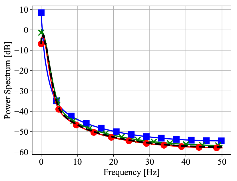
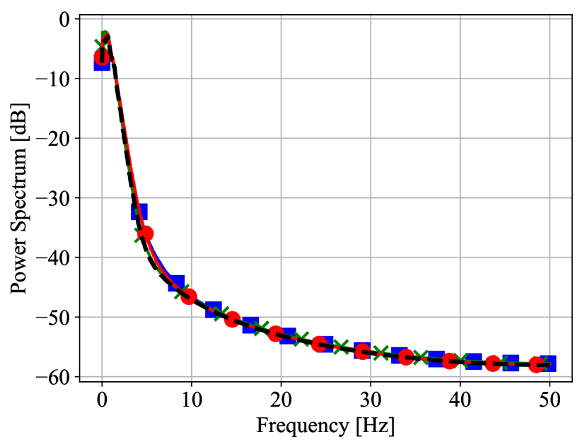
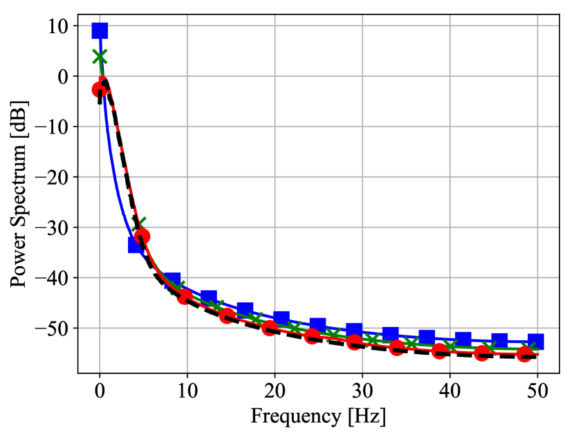
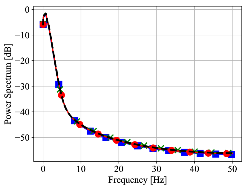
RC ; GRU ; LSTM ; Groundtruth ;
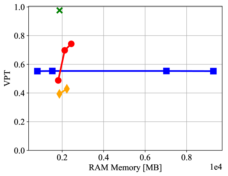
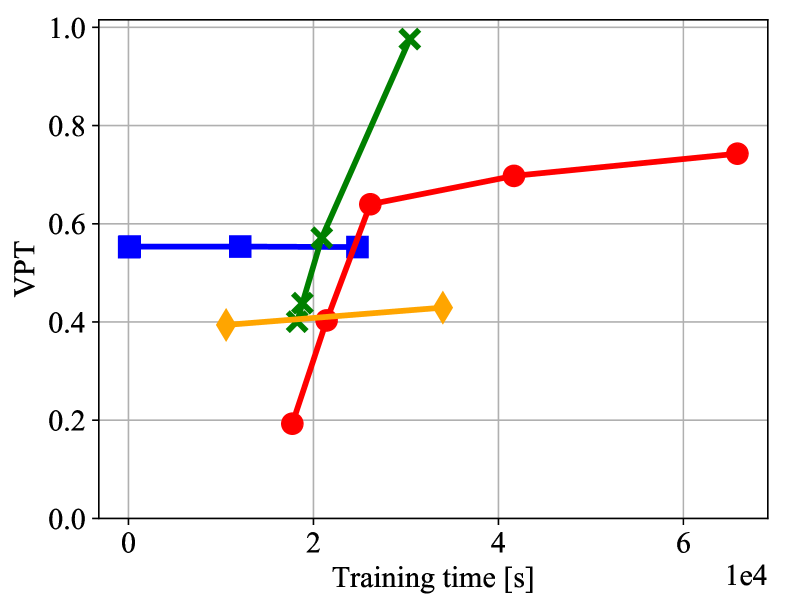
An important aspect of machine learning models is their scalability to high-dimensional systems and their requirements in terms of training time and memory utilization. Large memory requirements and/or high training times might hinder the application of the models in challenging scenarios, like high-performance applications in climate forecasting (Kurth et al., 2018). In Figure 6(a) and Figure 6(d), we present a Pareto front of the VPT with respect to the CPU RAM memory utilized to train the models with the highest VPT for each architecture for an input dimensions of (reduced order) and (full dimension) respectively. Figure 6(b) and Figure 6(e), show the corresponding Pareto fronts of the VPT with respect to the training time. In case of the full state space (), the RC is able to achieve superior VPT with smaller memory usage and vastly smaller training time than the other methods. However, in the case of reduced order information (), the BPTT algorithms (GRU and LSTM) are superior to the RC even when the latter is provided with one order of magnitude more memory.
Due to the fact that the RNN models are learning the recurrent connections, they are able to reach higher VPT when forecasting in the reduced order space without the need for large models. In contrast, in RC the maximum reservoir size (imposed by computer memory limitations) may not be sufficient to capture the dynamics of high-dimensional systems with reduced order information and non-local interactions. We argue that this is the reason why the RC models do not reach the performance of GRU/LSTM trained with Back-propagation (see Figure 6(a)).
At the same time, letting memory limitations aside, training of RC models requires the solution of a linear system of equations , with , and (see Appendix A). The Moore-Penrose method of solving this system, scales cubically with the reservoir size as it requires the inversion of a matrix with dimensions . We also tried an approximate iterative method termed LSQR based on diagonalization, without any significant influence on the training time. In contrast, the training time of an RNN is very difficult to estimate a priori, as convergence of the training method depends on initialization and various other hyperparameters and are not necessarily dependent on the size. That is why we observe a greater variation of the training time of RNN models. Similar results are obtained for , the interested reader is referred to the appendix.
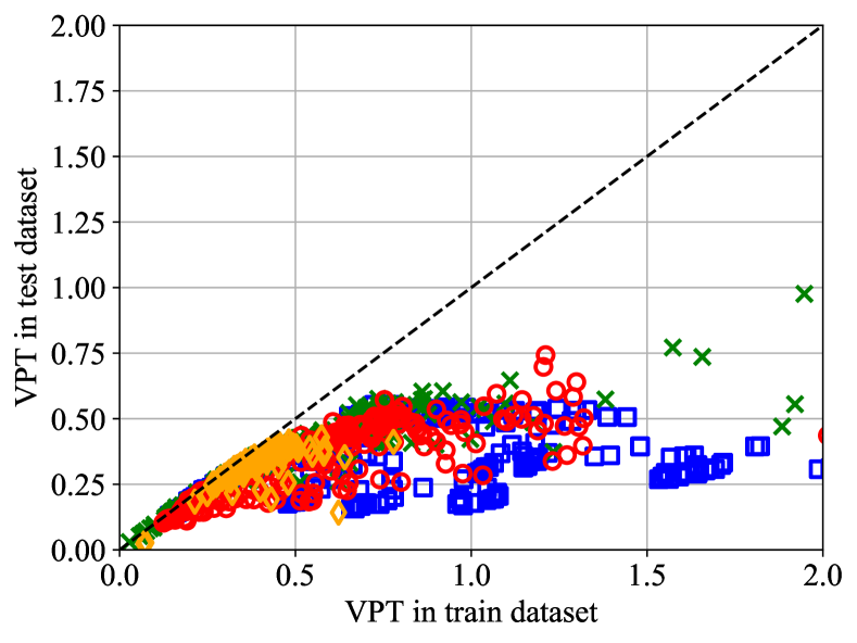
In the following, we evaluate to which extend the trained models overfit to the training data. For this reason, we measure the VPT in the training dataset and plot it against the VPT in the test dataset for every model we trained. This plot provides insight on the generalization error of the models. The results are shown in Figure 6(c), and Figure 6(f) for and . Ideally a model architecture that guards effectively against overfitting, exhibits a low generalization error, and should be represented by a point in this plot that is close to the identity line (zero generalization error). As the expressive power of a model increases, the model may fit better to the training data, but bigger models are more prone to memorizing the training dataset and overfitting (high generalization error). Such models would be represented by points on the right side of the plot. In the reduced order scenario, GRU and LSTM models lie closer to the identity line than RC models, exhibiting lower generalization errors. This is due to the validation-based early stopping routine utilized in the RNNs that guards effectively against overfitting.
We may alleviate the overfitting in RC by tuning the Tikhonov regularization parameter (). However, this requires to rerun the training for every other combination of hyperparameters. For the four tested values of the Tikhonov regularization parameter the RC models tend to exhibit higher generalization error compared to the RNNs trained with BBTT. We also tested more values , while keeping fixed the other hyperparameters, without any observable differences in the results.
However, in the full-order scenario, the RC models achieve superior forecasting accuracy and generalization ability as clearly depicted in Figure 6(f). Especially the additional regularization of the training procedure introduced by adding Gaussian noise in the data was decisive to achieve this result.
An example of an iterative forecast in the test dataset, is illustrated in Figure 7 for and .
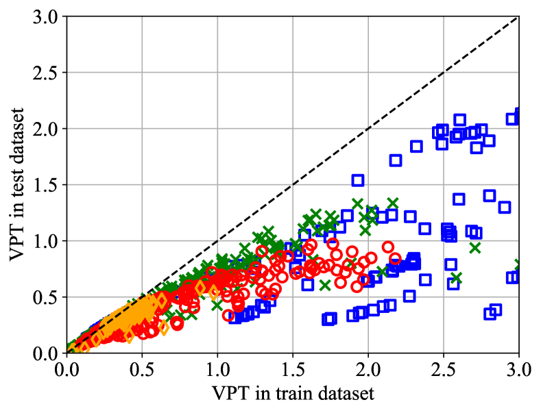
RC (or ) ; GRU (or ) ; LSTM (or ) ; Unit (or ) ; Ideal ;
GRU ; LSTM ; RC-6000 ; RC-9000 ; Unit ;
5 Parallel Forecasting Leveraging Local Interactions
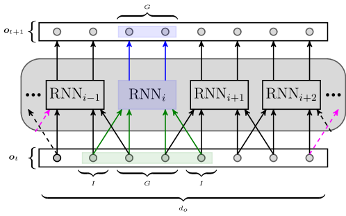
In spatially extended dynamical systems the state space (e.g., vorticity, velocity field, etc.) is high-dimensional (or even infinite dimensional), since an adequately fine grid is needed to resolve the relevant spatio-temporal scales of the dynamics. Even though RC and RNNs can be utilized for modeling and forecasting of these systems in the short-term, the RC and RNN methods described in Section 2 do not scale efficiently with the input dimension, i.e., as the dimensionality of the observable increases. Two limiting factor are the required time and RAM memory to train the model. As increases, the size of the reservoir network required to predict the system using only a single reservoir rises. This implies higher training times and more computational resources (RAM memory), which render the problem intractable for large values of . The same applies for RNNs. More limiting factors arise by taking the process of identification of optimal model hyperparameters into account, since loading, storing and processing a very large number of large models can be computationally infeasible. However, these scaling problems for large systems can be alleviated in case the system is characterized by local state interactions or translationally invariant dynamics. In the first case, as shown in Figure 8 the modeling and forecasting task can be parallelized by employing multiple individually trained networks forecasting locally in parallel exploiting the local interactions, while, if translation invariance also applies, the individual parallel networks can be identical and training of only one will be sufficient. This parallelization concept is utilized in RC in (Pathak et al., 2018a; Parlitz and Merkwirth, 2000). The idea dates back to local delay coordinates (Parlitz and Merkwirth, 2000). The model shares ideas from convolutional RNN architectures (Sainath et al., 2015; Shi et al., 2015) designed to capture local features that are translationally invariant in image and video processing tasks. In this section, we extend this parallelization scheme to RNNs and compare the efficiency of parallel RNNs and RCs in forecasting the state dynamics of the Lorenz-96 model and Kuramoto-Sivashinsky equation discretized in a fine grid.
5.1 Parallel Architecture
Assume that the observable is and each element of the observable is denoted by . In case of local interactions, the evolution of each element is affected by its spatially neighboring grid points. The elements are split into groups, each of which consisting of spatially neighboring elements such that . The parallel model employs RNNs, each of which is utilized to predict a spatially local region of the system observable indicated by the group elements . Each of the RNNs receives inputs from the elements it forecasts in addition to inputs from neighboring elements on the left and on the right, where is the interaction length. An example with and is illustrated in Figure 8.
During the training process, the networks can be trained independently. However, for long-term forecasting, a communication protocol has to be utilized as each network requires the predictions of neighboring networks to infer. In the case of a homogeneous system, where the dynamics are translation invariant, the training process can be drastically reduced by utilizing one single RNN and training it on data from all groups. The weights of this RNN are then copied to all other members of the network. In the following we assume that we have no knowledge of the underlying data generating mechanism and its properties, so we assume the data is not homogeneous.
5.2 Results on the Lorenz-96
In this section, we employ the parallel architecture to forecast the state dynamics of the Lorenz-96 system explained in Section 4.1 with a state dimension of . Note that in contrast to Section 4.2, we do not construct an observable and then forecast the reduced order dynamics. Instead, we leverage the local interactions in the state space and employ an ensemble of networks forecasting the local dynamics.
Instead of a single RNN model forecasting the dimensional global state (composed of the values of the state in the grid nodes), we consider separate RNN models, each forecasting the evolution of a dimensional local state (composed of the values of the state in grid nodes). In order to forecast the evolution of the local state, we take into account its interaction with grid nodes on its left and on its right. The group size of the parallel models is thus , while the interaction length is . As a consequence, each model receives at its input an dimensional state and forecasts the evolution of a local state composed from grid nodes. The size of the hidden state in RC is . Smaller networks of size are selected for GRU and LSTM. The rest of the hyperparameters are given in the appendix. Results for Unitary networks are omitted, as the identification of hyperparameters leading to stable iterative forecasting was computationally heavy and all trained models led to unstable systems that diverged after a few iterations.
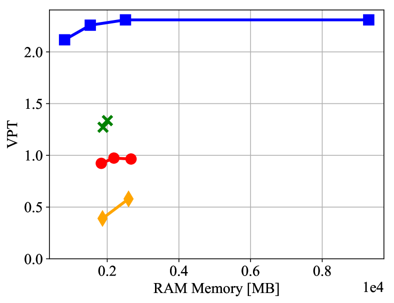
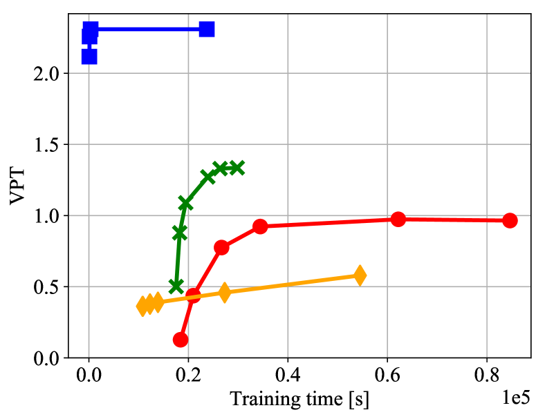
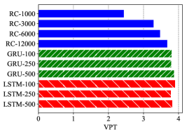
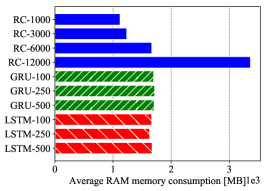
In Figure 9(a), we plot the VPT time of the RC and the BPTT networks. We find that RNN trained by BPTT achieve comparable predictions with RC, albeit using much smaller number hidden nodes (between 100 and 500 for BPTT vs 6000 to 12000 for RC). We remark that RC with 3000 and 6000 nodes have slightly lower VPT than GRU and LSTM but require significantly lower training times as shown in Figure 9(c). At the same time, using 12000 nodes for RC implies high RAM requirements, more than 3 GB per rank, as depicted in Figure 9(b).
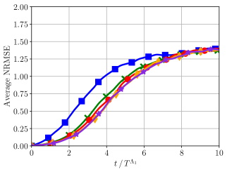
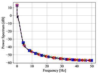
As elaborated in Section 4.2 and depicted in Figure 3(a), the VPT reached by large nonparallelized models that are forecasting the SVD modes of the system is approximately . We also verified that the nonparallelized models of Section 4.1 when forecasting the dimensional state containing local interactions instead of the modes of SVD, reach the same predictive performance. Consequently, as expected the VPT remains the same whether we are forecasting the state or the SVD modes as the system is deterministic. By exploiting the local interactions and employing the parallel networks, the VPT is increased from to as shown in Figure 9(a). The NRMSE error of the best performing hyperparameters is given in Figure 10(a). All models are able to reproduce the climate as the reconstructed power spectrum plotted in Figure 10(b) matches the true one. An example of an iterative prediction with LSTM, GRU and RC models starting from an initial condition in the test dataset is provided in Figure 11.
RC-1000 ; RC-6000 ; RC-12000 ; GRU-500 ; LSTM-100 ; Groundtruth ;
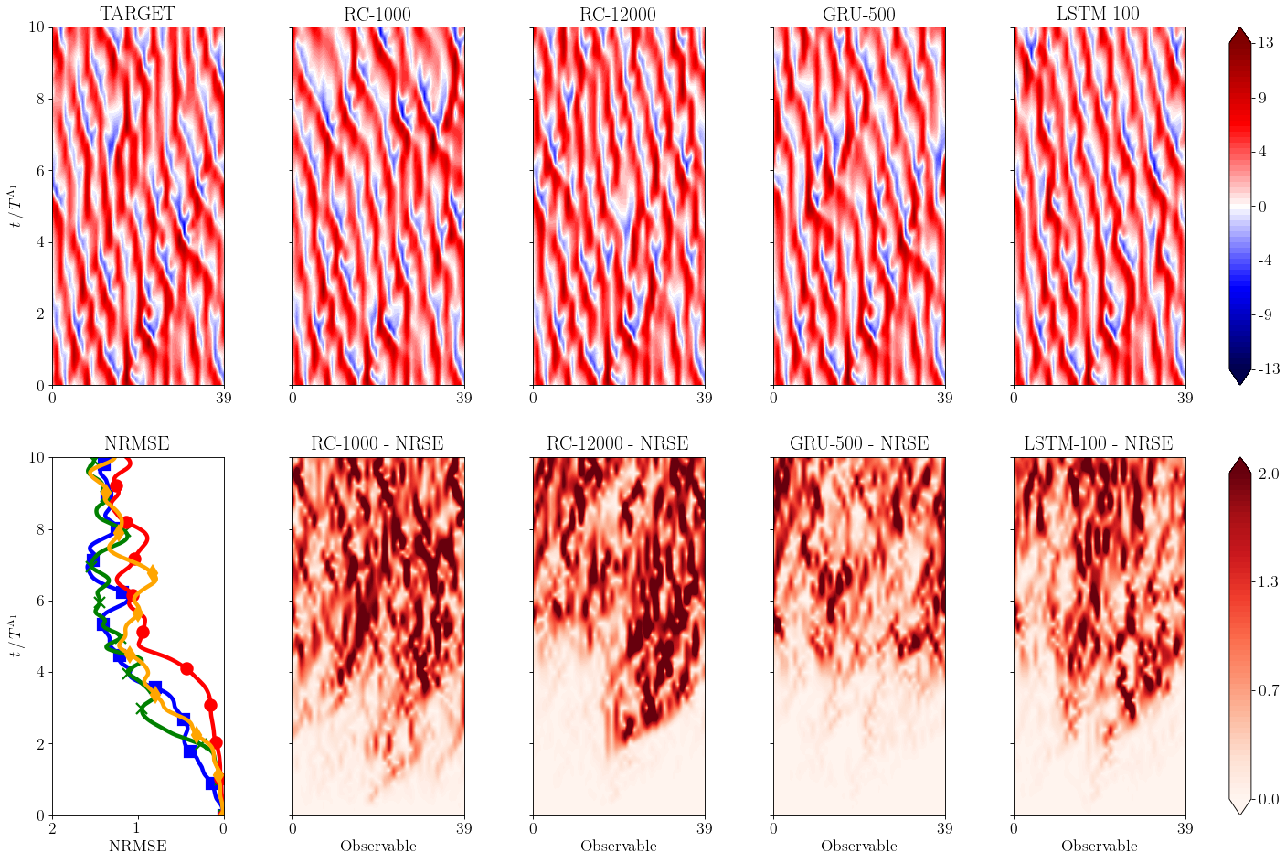
RC-1000 ; RC-12000 ; GRU-500 ; LSTM-100 ;
5.3 Kuramoto-Sivashinsky
The Kuramoto-Sivashinsky (KS) equation is a nonlinear partial differential equation of fourth order that is used as a turbulence model for various phenomena. It was derived by Kuramoto in (Kuramoto, 1978) to model the chaotic behavior of the phase gradient of a slowly varying amplitude in a reaction-diffusion type medium with negative viscosity coefficient. Moreover, Sivashinsky (Sivashinsky, 1977) derived the same equations when studying the instantaneous instabilities in a laminar flame front. For our study, we restrict ourselves to the one dimensional K-S equation
| (13) |
on the domain with periodic boundary conditions . The dimensionless boundary size directly affects the dimensionality of the attractor. For large values of , the attractor dimension scales linearly with (Manneville, 1984).
In order to spatially discretize Equation 13 we select a grid size with the number of nodes. Further, we denote with the value of at node . In the following, we select , and a grid of nodes. We discretize Equation 13 and solve it using the fourth-order method for stiff PDEs introduced in (Kassam and Trefethen, 2005) up to . This corresponds to samples. The first samples are truncated to avoid initial transients. The remaining data are divided to a training and a testing dataset of samples each. The observable is considered to be the dimensional state. The Lyapunov time of the system (see Section 3) is utilized as a reference timescale. We approximate it with the method of Pathak (Pathak et al., 2018a) for and it is found to be .
5.4 Results on the Kuramoto-Sivashinsky Equation
In this section, we present the results of the parallel models in the Kuramoto-Sivashinsky equation. The full system state is used as an observable, i.e., . The group-size of the parallel models is set to , while the interaction length is . The total number of groups is . Each member forecasts the evolution of state components, receiving at the input components in total. The size of the reservoir in RC is . For GRU and LSTM networks we vary . The rest of the hyperparameters are given in the appendix. Results on Unitary networks are omitted, as the configurations tried in this work led to unstable models diverging after a few time-steps in the iterative forecasting procedure.
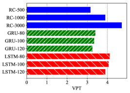
The results are summed up in the bar-plots in Figure 12. In Figure 12(a), we plot the VPT time of the models. LSTM models reach VPTs of , while GRU show an inferior predictive performance with VPTs of . An RC with reaches a VPT of , and an RC with modes reaches the VPT of LSTM models with a VPT of . Increasing the reservoir capacity of the RC to leads to a model exhibiting a VPT of . In this case, the large RC model shows slightly superior performance to GRU/LSTM. The low performance of GRU models can be attributed to the fact that in the parallel setting the probability that any RNN may converge to bad local minima rises, with a detrimental effect on the total predictive performance of the parallel ensemble. In case of spatially translational invariant systems, we could alleviate this problem by using one single network. Still, training the single network to data from all spatial locations would be expensive.
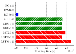
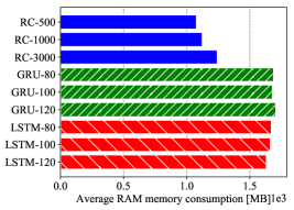
As depicted in Figure 12, the reservoir size of is enough for RC to reach and surpass the predictive performance of RNNs utilizing a similar amount of RAM memory and a much lower amount of training time as illustrated in Figure 12(b).
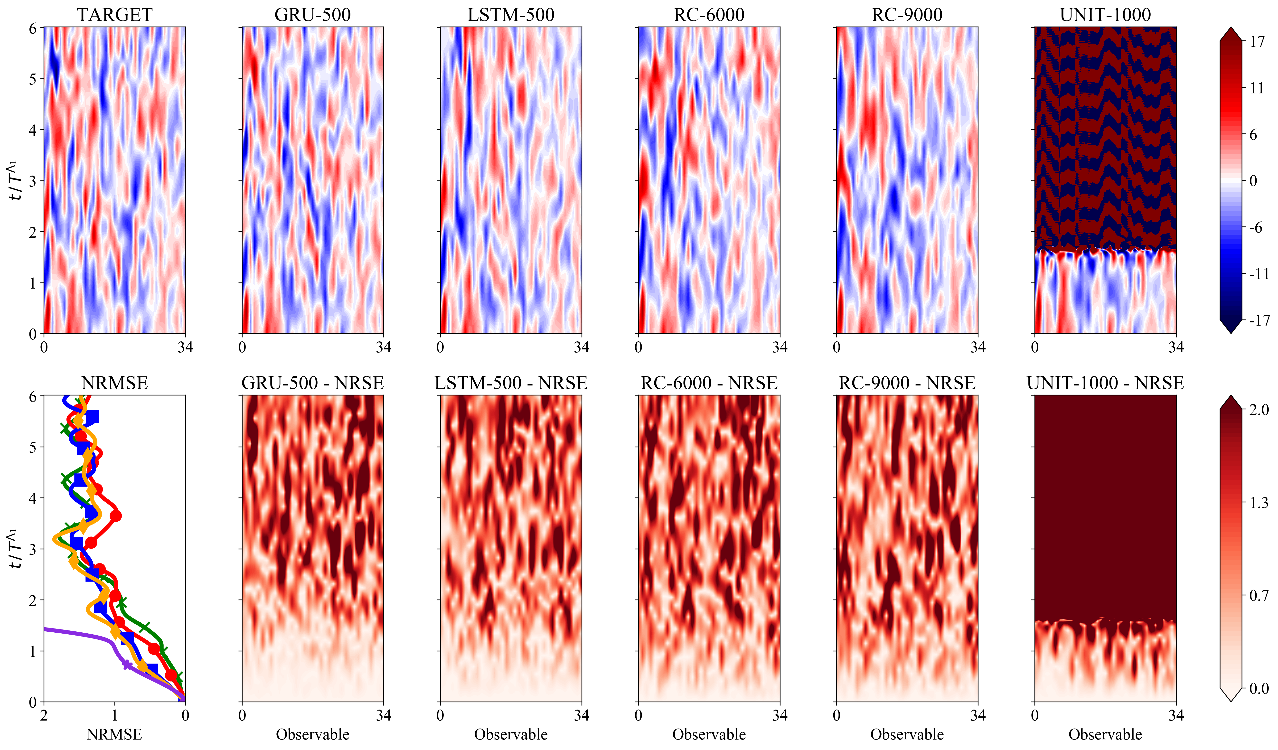
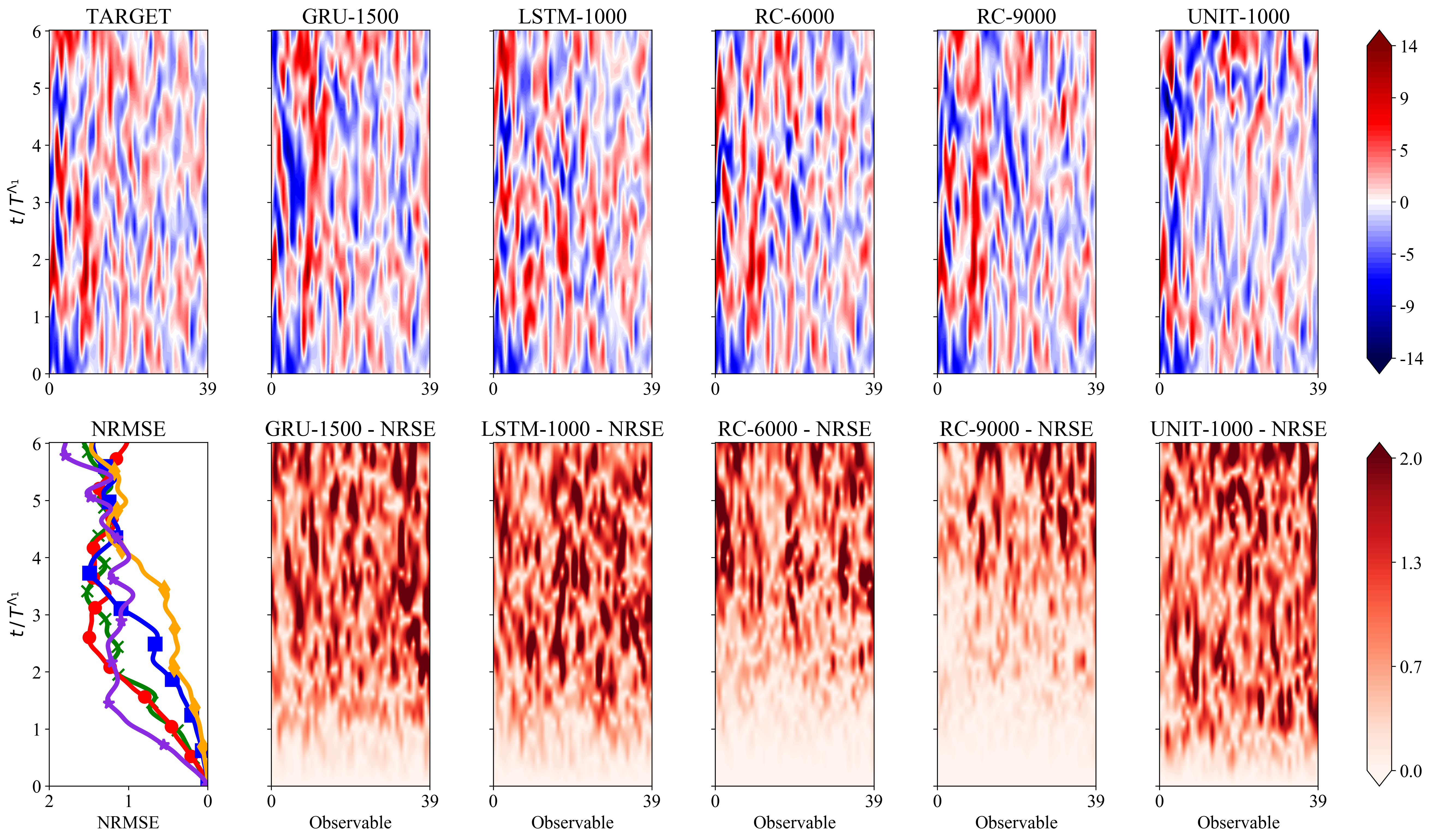
The evolution of the NRMSE is given in Figure 13(a). The predictive performance of a small LSTM network with hidden units, matches that of a large RC with hidden units. In Figure 13(b), the power spectrum of the predicted state dynamics of each model is plotted along with the true spectrum of the equations. The three models captured successfully the statistics of the system, as we observe a very good match. An example of an iterative prediction with LSTM, GRU and RC models starting from an initial condition in the test dataset is provided in Figure 14.
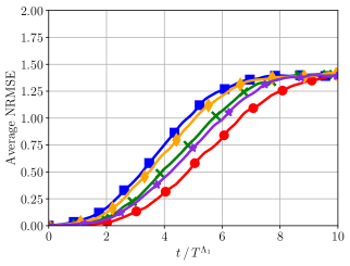
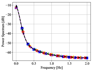
RC-500 ; RC-1000 ; RC-3000 ; GRU-80 ; LSTM-80 ; Groundtruth ;
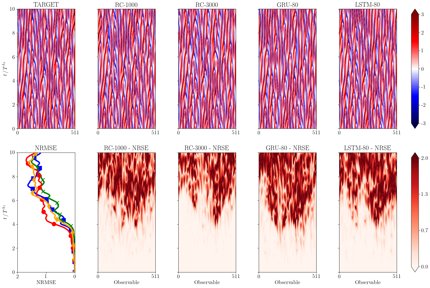
RC-1000 ; RC-3000 ; GRU-80 ; LSTM-80 ; Groundtruth ;
6 Calculation of Lyapunov Exponents in the Kuramoto-Sivashinsky Equation
The recurrent models utilized in this study can be used as surrogate models to calculate the Lyapunov exponents (LEs) of a dynamical system relying only on experimental time-series data. The LEs characterize the rate of separation if positive (or convergence if negative) of trajectories that are initialized infinitesimally close in the phase space. They can provide an estimate of the attractor dimension according to the Kaplan-Yorke formula (Kaplan and Yorke, 1979). Early efforts to solve the challenging problem of data-driven LE identification led to local approaches (Wolf et al., 1985; Sano and Sawada, 1985) that are computationally inexpensive at the cost of requiring a large amount of data. Other approaches fit a global model to the data (Maus and Sprott, 2013) and calculate the LE spectrum using the Jacobian algorithm. These approaches were applied to low-order systems.
A recent machine learning approach utilizes deep convolutional neural networks for LE and chaos identification, without estimation of the dynamics (Makarenko, 2018). An RC-RNN approach capable of uncovering the whole LE spetrum in high-dimensional dynamical systems is proposed in (Pathak et al., 2018a). The method is based on the training of a surrogate RC model to forecast the evolution of the state dynamics, and the calculation of the Lyapunov spectrum of the hidden state of this surrogate model. The RC method demonstrates excellent agreement for all positive Lyapunov exponents and many of the negative exponents for the KS equation with (Pathak et al., 2018a), alleviating the problem of spurious Lyapunov exponents of delay coordinate embeddings (Dechert and Gençay, 1996). We build on top of this work and demonstrate that a GRU trained with BPTT can reconstruct the Lyapunov spectrum accurately with lower error for all positive Lyapunov exponents at the cost of higher training times.
The Lyapunov spectrum of the KS equation is computed by solving the KS equations in the Fourier space with a fourth order time-stepping method called ETDRK4 (Kassam and Trefethen, 2005) and utilizing a QR decomposition approach as in (Pathak et al., 2018a). The Lyapunov spectrum of the RNN and RC surrogate models is computed based on the Jacobian of the hidden state dynamics along a reference trajectory, while Gram-Schmidt orthonormalization is utilized to alleviate numerical divergence. We employ a GRU-RNN over LSTM-RNN, due to the fact that the latter has two coupled hidden states, rendering the computation of the Lyapunov spectrum mathematically more involved and computationally more expensive. The interested reader can refer to the Appendix for the details of the method. The identified maximum LE is . In this work, a large RC with nodes is employed for LS calculation in the Kuramoto-Sivashinsky equation with parameter and grid points as in (Pathak et al., 2018a). The largest LE identified in this case is leading to a relative error of . In order to evaluate the efficiency of RNNs, we utilize a large GRU with hidden units. An iterative RNN roll-out of total time-steps was needed to achieve convergence of the spectrum. The largest Lyapunov exponent identified by the GRU is reducing the error to . Both surrogate models identify the correct Kaplan-Yorke dimension , which is the largest LE such that .
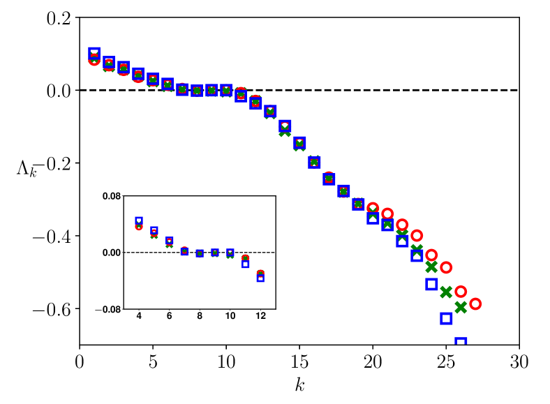
The first Lyapunov exponents computed the GRU, RC as well as using the true equations of the Kuramoto-Sivashinsky are plotted in Figure 15. We observe a good match between the positive Lyapunov exponents by both GRU and RC surrogates. The positive Lyapunov exponents are characteristic of chaotic behavior. However, the zero Lyapunov exponents and cannot be captured neither with RC nor with RNN surrogates. This is also observed in RC in (Pathak et al., 2018a), and apparently the GRU surrogate employed in this work do not alleviate the problem. In Figure 15(b), we augment the RC and the GRU spectrum with these two additional exponents to illustrate that there is an excellent agreement between the true LE and the augmented LS identified by the surrogate models.
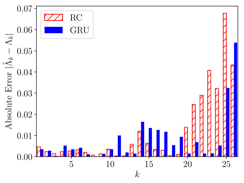
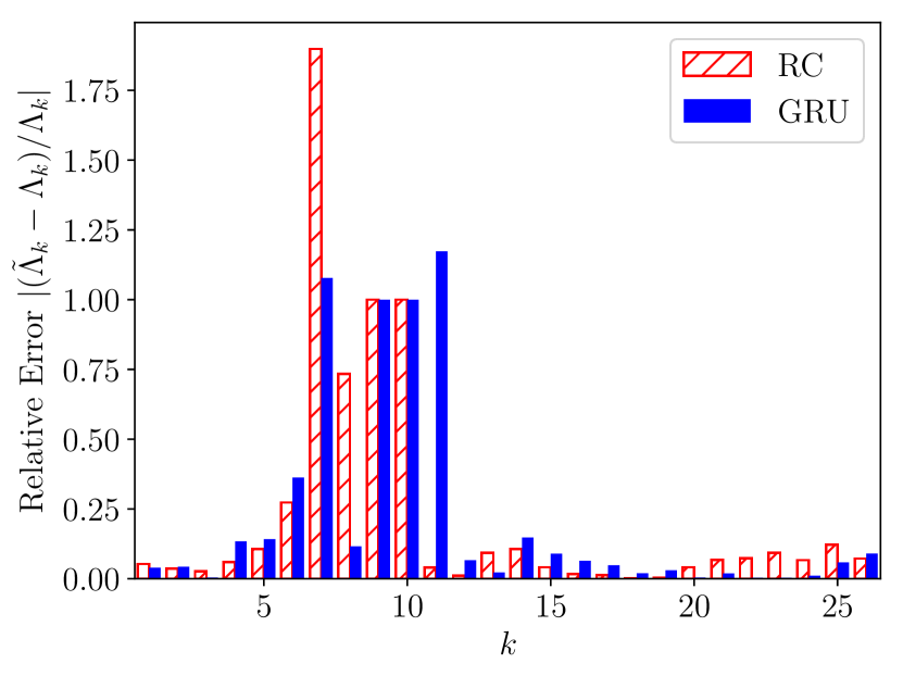
The relative and absolute errors in the spectrum calculation is illustrated in Figure 16. After augmenting with these zero LE, we get a mean absolute error of for RC and for GRU. The mean relative error is for RC, and for GRU. As a conclusion, GRU in par with RC networks can be used to replicate the chaotic behavior of a reference system and calculate the Lyapunov spectrum accurately.
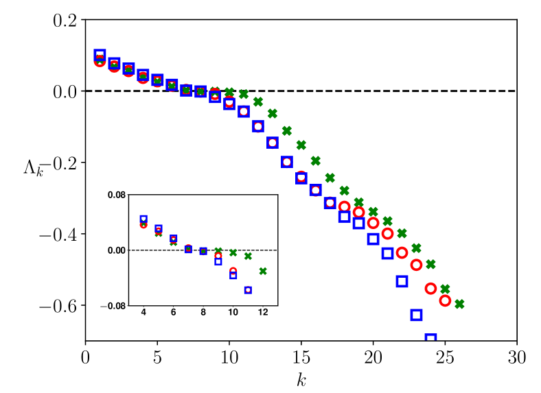
True ; RC ; GRU ;
7 Conclusions
In this work, we employed several variants of recurrent neural networks and reservoir computing to forecast the dynamics of chaotic systems. We present a comparative study based on their efficiency in capturing temporal dependencies, evaluate how they scale to systems with high-dimensional state space, and how to guard against overfitting. We highlight the advantages and limitations of these methods and elucidate their applicability to forecasting spatiotemporal dynamics.
We considered three different types of RNN cells that alleviate the well-known vanishing and exploding gradient problem in Back-propagation through time training (BPTT), namely LSTM, GRU and Unitary cells. We benchmarked these networks against reservoir computers with random hidden to hidden connection weights, whose training procedure amounts to least square regression on the output weights.
The efficiency of the models in capturing temporal dependencies in the reduced order state space is evaluated on the Lorenz-96 system in two different forcing regimes , by constructing a reduced order observable using Singular Value Decomposition (SVD) and keeping the most energetic modes. Even though this forecasting task is challenging due to (1) chaotic dynamics and (2) reduced order information, LSTM and GRU show superior forecasting ability to RC utilizing similar amounts of memory at the cost of higher training times. GRU and LSTM models demonstrate stable behavior in the iterative forecasting procedure in the sense that the forecasting error usually does not diverge, in stark contrast to RC and Unitary forecasts. Large RC models tend to overfit easier than LSTM/GRU models, as the latter are utilizing validation-based early stopping and regularization techniques (e.g., Zoneout, Dropout) that guard against overfitting which are not directly applicable to RC. Validation in RC amounts to tuning an additional hyperparameter, the Tikhonov regularization. However, RC shows excellent forecasting efficiency when the full state of the system is observed, outperforming all other models by a wide margin, while also reproducing the frequency spectrum of the underlying dynamics.
RNNs and RC both suffer from scalability problems in high-dimensional systems, as the required hidden state size to capture the high-dimensional dynamics can become prohibitively large especially with respect to the computational expense of training. In order to scale the models to high-dimensional systems we employ a parallelization scheme that exploits the local interactions in the state of a dynamical system. As a reference, we consider the Lorenz-96 system and the Kuramoto-Sivashinsky equation, and we train parallel RC, GRU, and LSTM models of various sizes. Iterative forecasting with parallel Unitary models diverged after a few timesteps in both systems. Parallel GRU, LSTM and RC networks reproduced the long-term attractor climate, as well as the power spectrum of the state of the Lorenz-96 and the Kuramoto-Sivashinsky equation matched with the predicted ones.
In the Lorenz-96 and the Kuramoto-Sivashinsky equation, the parallel LSTM and GRU models exhibited similar predictive performance compared to the parallel RC. The memory requirements of the models are comparable. RC networks require large reservoirs with nodes per member to reach the predictive performance of parallel GRU/LSTM with a few hundred nodes, but their training time is significantly lower.
Last but not least, we evaluated and compared the efficiency of GRU and RC networks in capturing the Lyapunov spectrum of the KS equation. The positive Lyapunov exponents are captured accurately by both RC and GRU. Both networks cannot reproduce two zero LEs and . When these two are discarded from the spectrum, GRU and RC networks show comparable accuracy in terms of relative and absolute error of the Lyapunov spectrum.
Further investigation on the underlying reasons why the RNNs and RC cannot capture the zero Lyapunov exponents is a matter of ongoing work. Another interesting direction could include studying the memory capacity of the networks. This could offer more insight into which architecture and training method is appropriate for tasks with long-term dependencies. Moreover, we plan to investigate a coupling of the two training approaches to further improve their predictive performance, for example a network can utilize both RC and LSTM computers to identify the input to output mapping. While the weights of the RC are initialized randomly to satisfy the echo state property, the output weights alongside with the LSTM weights can be optimized by back-propagation. This approach, although more costly, might achieve higher efficiency, as the LSTM is used as a residual model correcting the error that a plain RC would have.
Although we considered a batched version of RC training to reduce the memory requirements, further research is needed to alleviate the memory burden associated with the matrix inversion (see Appendix A,Equation 15) and the numerical problems associated with the eigenvalue decomposition of the sparse weight matrix.
Further directions could be the initialization of RNN weights with RC based heuristics based on the echo state property and fine-tuning with BPTT. Another promising direction is to evaluate the models in terms of the amount of data needed to learn the system dynamics. This is possible for the plain cell RNN, where the heuristics are directly applicable. However, in more complex architectures like the LSTM or the GRU, more sophisticated initialization schemes that ensure some form of echo state property have to be investigated. The computational cost of training networks of the size of RC with back-propagation is also challenging. This hybrid training method is an interesting future direction.
One topic not covered in this work, is invertibility of the models, when forecasting the full state dynamics. Non-invertible models like the RNNs trained in this work, may suffer from spurious dynamics not present the training data and the underlying governing equations (Gicquel et al., 1998; Frouzakis et al., 1997). Invertible RNNs may constitute a promising alternative to further improve accurate short-term prediction and capturing of the long-term dynamics.
In conclusion, recurrent neural networks for data-driven surrogate modeling and forecasting of chaotic systems can efficiently be used to model high-dimensional dynamical systems, can be parallelized alleviating scaling problems and constitute a promising research subject that requires further analysis.
8 Data and Code
The code and data will be available upon publication in the following link https://github.com/pvlachas/RNN to assist reproducibility of the results. The software was written in Python utilizing Tensorflow (Abadi et al., 2016) and Pytorch (Paszke et al., 2017) for automatic differentiation and the design of the neural network architectures.
9 Acknowledgments
We thank Guido Novati for helpful discussions and valuable feedback on this manuscript. Moreover, we would like to acknowledge the time and effort of Prof. Herbert Jaeger along with two anonymous reviewers whose insightful and thorough feedback led to substantial improvements of the manuscript. TPS has been supported through the ARO-MURI grant W911NF-17-1-0306. This work has been supported at UMD by DARPA under grant number DMS51813027. We are also thankful to the Swiss National Supercomputing Centre (CSCS) providing the necessary computational resources under Projects s929.
References
- Abadi et al. (2016) Abadi, M., Barham, P., Chen, J., Chen, Z., Davis, A., Dean, J., Devin, M., Ghemawat, S., Irving, G., Isard, M., Kudlur, M., Levenberg, J., Monga, R., Moore, S., Murray, D.G., Steiner, B., Tucker, P., Vasudevan, V., Warden, P., Wicke, M., Yu, Y., Zheng, X., 2016. Tensorflow: A system for large-scale machine learning, in: 12th USENIX Symposium on Operating Systems Design and Implementation (OSDI 16), pp. 265–283. URL: https://www.usenix.org/system/files/conference/osdi16/osdi16-abadi.pdf.
- Abarbanel (2012) Abarbanel, H., 2012. Analysis of observed chaotic data. Springer Science & Business Media.
- Aksamit et al. (2019) Aksamit, N.O., Sapsis, T.P., Haller, G., 2019. Machine-learning ocean dynamics from lagrangian drifter trajectories. arXiv preprint arXiv:1909.12895 .
- Antonik et al. (2017) Antonik, P., Haelterman, M., Massar, S., 2017. Brain-inspired photonic signal processor for generating periodic patterns and emulating chaotic systems. Phys. Rev. Applied 7, 054014. URL: https://link.aps.org/doi/10.1103/PhysRevApplied.7.054014, doi:10.1103/PhysRevApplied.7.054014.
- Arjovsky et al. (2016) Arjovsky, M., Shah, A., Bengio, Y., 2016. Unitary evolution recurrent neural networks, in: Proceedings of the 33rd International Conference on International Conference on Machine Learning - Volume 48, JMLR.org. pp. 1120–1128. URL: http://dl.acm.org/citation.cfm?id=3045390.3045509.
- Bengio et al. (1994) Bengio, Y., Simard, P., Frasconi, P., 1994. Learning long-term dependencies with gradient descent is difficult. Trans. Neur. Netw. 5, 157–166. URL: http://dx.doi.org/10.1109/72.279181, doi:10.1109/72.279181.
- Bianchi et al. (2017) Bianchi, F.M., Maiorino, E., Kampffmeyer, M.C., Rizzi, A., Jenssen, R., 2017. An overview and comparative analysis of recurrent neural networks for short term load forecasting. CoRR abs/1705.04378. URL: http://arxiv.org/abs/1705.04378, arXiv:1705.04378.
- Bradley and Kantz (2015) Bradley, E., Kantz, H., 2015. Nonlinear time-series analysis revisited. Chaos: An Interdisciplinary Journal of Nonlinear Science 25, 097610. doi:10.1063/1.4917289.
- Brockman et al. (2016) Brockman, G., Cheung, V., Pettersson, L., Schneider, J., Schulman, J., Tang, J., Zaremba, W., 2016. Openai gym. arXiv preprint arXiv:1606.01540 .
- Brunton et al. (2020) Brunton, S.L., Noack, B.R., Koumoutsakos, P., 2020. Machine learning for fluid mechanics. Annual Review of Fluid Mechanics 52, 477--508.
- Cao et al. (1995) Cao, L., Hong, Y., Fang, H., He, G., 1995. Predicting chaotic time series with wavelet networks. Physica D: Nonlinear Phenomena 85, 225 -- 238. URL: http://www.sciencedirect.com/science/article/pii/016727899500119O, doi:https://doi.org/10.1016/0167-2789(95)00119-O.
- Cho et al. (2014) Cho, K., van Merrienboer, B., Gulcehre, C., Bahdanau, D., Bougares, F., Schwenk, H., Bengio, Y., 2014. Learning phrase representations using rnn encoder--decoder for statistical machine translation, in: Proceedings of the 2014 Conference on Empirical Methods in Natural Language Processing (EMNLP), Association for Computational Linguistics. pp. 1724--1734. URL: http://aclweb.org/anthology/D14-1179, doi:10.3115/v1/D14-1179.
- Chung et al. (2014) Chung, J., Gulcehre, C., Cho, K., Bengio, Y., 2014. Empirical evaluation of gated recurrent neural networks on sequence modeling, in: NIPS 2014 Workshop on Deep Learning, December 2014.
- Dalcín et al. (2008) Dalcín, L., Paz, R., Storti, M., D’Elía, J., 2008. Mpi for python: Performance improvements and mpi-2 extensions. Journal of Parallel and Distributed Computing 68, 655--662.
- Dalcin et al. (2011) Dalcin, L.D., Paz, R.R., Kler, P.A., Cosimo, A., 2011. Parallel distributed computing using python. Advances in Water Resources 34, 1124--1139.
- Dechert and Gençay (1996) Dechert, W.D., Gençay, R., 1996. The topological invariance of Lyapunov exponents in embedded dynamics. Physica D Nonlinear Phenomena 90, 40--55. doi:10.1016/0167-2789(95)00225-1.
- Dong et al. (2015) Dong, D., Wu, H., He, W., Yu, D., Wang, H., 2015. Multi-task learning for multiple language translation, in: Proceedings of the 53rd Annual Meeting of the Association for Computational Linguistics and the 7th International Joint Conference on Natural Language Processing (Volume 1: Long Papers), pp. 1723--1732.
- Dreyfus (1962) Dreyfus, S., 1962. The numerical solution of variational problems. Journal of Mathematical Analysis and Applications 5, 30 -- 45.
- Elman (1990) Elman, J.L., 1990. Finding structure in time. COGNITIVE SCIENCE 14, 179--211.
- Esteva et al. (2017) Esteva, A., Kuprel, B., Novoa, R.A., Ko, J., Swetter, S.M., Blau, H.M., Thrun, S., 2017. Dermatologist-level classification of skin cancer with deep neural networks. Nature 542, 115.
- Faller and Schreck (1997) Faller, W.E., Schreck, S.J., 1997. Unsteady fluid mechanics applications of neural networks. Journal of Aircraft 34, 48--55. doi:10.2514/2.2134.
- Frouzakis et al. (1997) Frouzakis, C.E., Gardini, L., Kevrekidis, I.G., Millerioux, G., Mira, C., 1997. On some properties of invariant sets of two-dimensional noninvertible maps. International Journal of Bifurcation and Chaos 7, 1167--1194.
- Gal and Ghahramani (2016) Gal, Y., Ghahramani, Z., 2016. A theoretically grounded application of dropout in recurrent neural networks, in: Lee, D.D., Sugiyama, M., Luxburg, U.V., Guyon, I., Garnett, R. (Eds.), Advances in Neural Information Processing Systems 29. Curran Associates, Inc., pp. 1019--1027. URL: http://papers.nips.cc/paper/6241-a-theoretically-grounded-application-of-dropout-in-recurrent-neural-networks.pdf.
- Gicquel et al. (1998) Gicquel, N., Anderson, J., Kevrekidis, I., 1998. Noninvertibility and resonance in discrete-time neural networks for time-series processing. Physics Letters A 238, 8--18.
- Glorot and Bengio (2010) Glorot, X., Bengio, Y., 2010. Understanding the difficulty of training deep feedforward neural networks, in: Proceedings of the thirteenth international conference on artificial intelligence and statistics, pp. 249--256.
- Gneiting and Raftery (2005) Gneiting, T., Raftery, A.E., 2005. Weather forecasting with ensemble methods. Science 310, 248--249.
- Gonon and Ortega (2019) Gonon, L., Ortega, J.P., 2019. Reservoir computing universality with stochastic inputs. IEEE transactions on neural networks and learning systems .
- Goodfellow et al. (2016) Goodfellow, I., Bengio, Y., Courville, A., 2016. Deep Learning. MIT Press.
- Graves and Jaitly (2014) Graves, A., Jaitly, N., 2014. Towards end-to-end speech recognition with recurrent neural networks, in: International conference on machine learning, pp. 1764--1772.
- Greff et al. (2016) Greff, K., Srivastava, R.K., Koutník, J., Steunebrink, B.R., Schmidhuber, J., 2016. Lstm: A search space odyssey. IEEE transactions on neural networks and learning systems 28, 2222--2232.
- Grigoryeva and Ortega (2018) Grigoryeva, L., Ortega, J.P., 2018. Echo state networks are universal. Neural Networks 108, 495--508.
- Ha and Schmidhuber (2018) Ha, D., Schmidhuber, J., 2018. World models. arXiv preprint arXiv:1803.10122 .
- Hassabis et al. (2017) Hassabis, D., Kumaran, D., Summerfield, C., Botvinick, M., 2017. Neuroscience-inspired artificial intelligence. Neuron 95, 245--258.
- Haynes et al. (2015) Haynes, N.D., Soriano, M.C., Rosin, D.P., Fischer, I., Gauthier, D.J., 2015. Reservoir computing with a single time-delay autonomous boolean node. Phys. Rev. E 91, 020801. URL: https://link.aps.org/doi/10.1103/PhysRevE.91.020801, doi:10.1103/PhysRevE.91.020801.
- He et al. (2016) He, K., Zhang, X., Ren, S., Sun, J., 2016. Deep residual learning for image recognition. 2016 IEEE Conference on Computer Vision and Pattern Recognition (CVPR) , 770--778.
- Hochreiter (1998) Hochreiter, S., 1998. The vanishing gradient problem during learning recurrent neural nets and problem solutions. International Journal of Uncertainty, Fuzziness and Knowledge-Based Systems 6, 107--116. doi:10.1142/S0218488598000094.
- Hochreiter and Schmidhuber (1997) Hochreiter, S., Schmidhuber, J., 1997. Long short-term memory. Neural Comput. 9, 1735--1780. URL: http://dx.doi.org/10.1162/neco.1997.9.8.1735, doi:10.1162/neco.1997.9.8.1735.
- Jaeger and Haas (2004) Jaeger, H., Haas, H., 2004. Harnessing nonlinearity: Predicting chaotic systems and saving energy in wireless communication. Science 304, 78--80. URL: http://science.sciencemag.org/content/304/5667/78, doi:10.1126/science.1091277, arXiv:http://science.sciencemag.org/content/304/5667/78.full.pdf.
- Jiang and Lai (2019) Jiang, J., Lai, Y.C., 2019. Model-free prediction of spatiotemporal dynamical systems with recurrent neural networks: Role of network spectral radius. Phys. Rev. Research 1, 033056. URL: https://link.aps.org/doi/10.1103/PhysRevResearch.1.033056, doi:10.1103/PhysRevResearch.1.033056.
- Jing et al. (2017) Jing, L., Shen, Y., Dubcek, T., Peurifoy, J., Skirlo, S.A., LeCun, Y., Tegmark, M., Soljacic, M., 2017. Tunable efficient unitary neural networks (EUNN) and their application to rnns, in: ICML, PMLR. pp. 1733--1741.
- Jozefowicz et al. (2015) Jozefowicz, R., Zaremba, W., Sutskever, I., 2015. An empirical exploration of recurrent network architectures, in: Proceedings of the 32Nd International Conference on International Conference on Machine Learning - Volume 37, JMLR.org. pp. 2342--2350. URL: http://dl.acm.org/citation.cfm?id=3045118.3045367.
- Kantz and Schreiber (1997) Kantz, H., Schreiber, T., 1997. Nonlinear Time Series Analysis. Cambridge University Press, New York, NY, USA.
- Kaplan and Yorke (1979) Kaplan, J.L., Yorke, J.A., 1979. Chaotic behavior of multidimensional difference equations, in: Peitgen, H.O., Walther, H.O. (Eds.), Functional Differential Equations and Approximation of Fixed Points, Springer Berlin Heidelberg, Berlin, Heidelberg. pp. 204--227.
- Kassam and Trefethen (2005) Kassam, A., Trefethen, L., 2005. Fourth-order time-stepping for stiff pdes. SIAM Journal on Scientific Computing 26, 1214--1233. doi:10.1137/S1064827502410633.
- Kingma and Ba (2015) Kingma, D.P., Ba, J., 2015. Adam: A method for stochastic optimization, in: 3rd International Conference on Learning Representations, ICLR 2015, San Diego, CA, USA, May 7-9, 2015, Conference Track Proceedings.
- Koopman (1931) Koopman, B.O., 1931. Hamiltonian systems and transformation in hilbert space. Proceedings of the National Academy of Sciences of the United States of America 17, 315.
- Krueger et al. (2017) Krueger, D., Maharaj, T., Kramár, J., Pezeshki, M., Ballas, N., Ke, N.R., Goyal, A., Bengio, Y., Courville, A.C., Pal, C.J., 2017. Zoneout: Regularizing rnns by randomly preserving hidden activations, in: 5th International Conference on Learning Representations, ICLR 2017, Toulon, France, April 24-26, 2017, Conference Track Proceedings. URL: https://openreview.net/forum?id=rJqBEPcxe.
- Kuramoto (1978) Kuramoto, Y., 1978. Diffusion-Induced Chaos in Reaction Systems. Progress of Theoretical Physics Supplement 64, 346--367. URL: https://dx.doi.org/10.1143/PTPS.64.346, doi:10.1143/PTPS.64.346, arXiv:http://oup.prod.sis.lan/ptps/article-pdf/doi/10.1143/PTPS.64.346/5293041/64-346.pdf.
- Kurth et al. (2018) Kurth, T., Treichler, S., Romero, J., Mudigonda, M., Luehr, N., Phillips, E., Mahesh, A., Matheson, M., Deslippe, J., Fatica, M., et al., 2018. Exascale deep learning for climate analytics, in: SC18: International Conference for High Performance Computing, Networking, Storage and Analysis, IEEE. pp. 649--660.
- Lapedes and Farber (1987) Lapedes, A., Farber, R., 1987. Nonlinear signal processing using neural networks: Prediction and system modelling. Technical Report.
- Laptev et al. (2017) Laptev, N., Yosinski, J., Li, L.E., Smyl, S., 2017. Time-series extreme event forecasting with neural networks at uber.
- Larger et al. (2017) Larger, L., Baylón-Fuentes, A., Martinenghi, R., Udaltsov, V.S., Chembo, Y.K., Jacquot, M., 2017. High-speed photonic reservoir computing using a time-delay-based architecture: Million words per second classification. Phys. Rev. X 7, 011015. URL: https://link.aps.org/doi/10.1103/PhysRevX.7.011015, doi:10.1103/PhysRevX.7.011015.
- Larger et al. (2012) Larger, L., Soriano, M.C., Brunner, D., Appeltant, L., Gutierrez, J.M., Pesquera, L., Mirasso, C.R., Fischer, I., 2012. Photonic information processing beyond turing: an optoelectronic implementation of reservoir computing. Opt. Express 20, 3241--3249. URL: http://www.opticsexpress.org/abstract.cfm?URI=oe-20-3-3241, doi:10.1364/OE.20.003241.
- Linnainmaa (1976) Linnainmaa, S., 1976. Taylor expansion of the accumulated rounding error. BIT Numerical Mathematics 16, 146--160. doi:10.1007/BF01931367.
- Lorenz (1995) Lorenz, E., 1995. Predictability: a problem partly solved, in: Seminar on Predictability, 4-8 September 1995, ECMWF. ECMWF, Shinfield Park, Reading. pp. 1--18. URL: https://www.ecmwf.int/node/10829.
- Lu et al. (2018) Lu, Z., Hunt, B.R., Ott, E., 2018. Attractor reconstruction by machine learning. Chaos: An Interdisciplinary Journal of Nonlinear Science 28, 061104.
- Lukoševičius (2012) Lukoševičius, M., 2012. A practical guide to applying echo state networks, in: Neural Networks: Tricks of the Trade.
- Lukoševičius and Jaeger (2009) Lukoševičius, M., Jaeger, H., 2009. Reservoir computing approaches to recurrent neural network training. Computer Science Review 3, 127 -- 149. doi:https://doi.org/10.1016/j.cosrev.2009.03.005.
- Lusch et al. (2018) Lusch, B., Kutz, J.N., Brunton, S.L., 2018. Deep learning for universal linear embeddings of nonlinear dynamics. Nature communications 9, 4950.
- Maass et al. (2002) Maass, W., Natschläger, T., Markram, H., 2002. Real-time computing without stable states: A new framework for neural computation based on perturbations. Neural Comput. 14, 2531--2560. URL: http://dx.doi.org/10.1162/089976602760407955, doi:10.1162/089976602760407955.
- Makarenko (2018) Makarenko, A.V., 2018. Deep convolutional neural networks for chaos identification in signal processing, in: 2018 26th European Signal Processing Conference (EUSIPCO), IEEE. pp. 1467--1471.
- Manneville (1984) Manneville, P., 1984. Macroscopic modelling of turbulent flows, proceedings of a workshop held at inria, sophia-antipolis, france, 1984. Lecture Notes in Physics 230, 319--326.
- Maus and Sprott (2013) Maus, A., Sprott, J.C., 2013. Evaluating lyapunov exponent spectra with neural networks. Chaos, Solitons and Fractals 51, 13--21. doi:10.1016/j.chaos.2013.03.001.
- Mnih et al. (2015) Mnih, V., Kavukcuoglu, K., Silver, D., Rusu, A.A., Veness, J., Bellemare, M.G., Graves, A., Riedmiller, M., Fidjeland, A.K., Ostrovski, G., et al., 2015. Human-level control through deep reinforcement learning. Nature 518, 529.
- Neofotistos et al. (2019) Neofotistos, G., Mattheakis, M., Barmparis, G.D., Hizanidis, J., Tsironis, G.P., Kaxiras, E., 2019. Machine learning with observers predicts complex spatiotemporal behavior. Frontiers in Physics 7, 24. URL: https://www.frontiersin.org/article/10.3389/fphy.2019.00024, doi:10.3389/fphy.2019.00024.
- Ott (2002) Ott, E., 2002. Chaos in Dynamical Systems. 2 ed., Cambridge University Press. doi:10.1017/CBO9780511803260.
- Parlitz and Merkwirth (2000) Parlitz, U., Merkwirth, C., 2000. Prediction of spatiotemporal time series based on reconstructed local states. Phys. Rev. Lett. 84, 1890--1893. URL: https://link.aps.org/doi/10.1103/PhysRevLett.84.1890, doi:10.1103/PhysRevLett.84.1890.
- Pascanu et al. (2013) Pascanu, R., Mikolov, T., Bengio, Y., 2013. On the difficulty of training recurrent neural networks, in: Proceedings of the 30th International Conference on International Conference on Machine Learning - Volume 28, JMLR.org. pp. III--1310--III--1318. URL: http://dl.acm.org/citation.cfm?id=3042817.3043083.
- Paszke et al. (2017) Paszke, A., Gross, S., Chintala, S., Chanan, G., Yang, E., DeVito, Z., Lin, Z., Desmaison, A., Antiga, L., Lerer, A., 2017. Automatic differentiation in pytorch .
- Pathak et al. (2018a) Pathak, J., Hunt, B., Girvan, M., Lu, Z., Ott, E., 2018a. Model-free prediction of large spatiotemporally chaotic systems from data: A reservoir computing approach. Phys. Rev. Lett. 120, 024102. URL: https://link.aps.org/doi/10.1103/PhysRevLett.120.024102, doi:10.1103/PhysRevLett.120.024102.
- Pathak et al. (2017) Pathak, J., Lu, Z., Hunt, B.R., Girvan, M., Ott, E., 2017. Using machine learning to replicate chaotic attractors and calculate lyapunov exponents from data. Chaos: An Interdisciplinary Journal of Nonlinear Science 27, 121102. doi:10.1063/1.5010300.
- Pathak et al. (2018b) Pathak, J., Wikner, A., Fussell, R., Chandra, S., Hunt, B.R., Girvan, M., Ott, E., 2018b. Hybrid forecasting of chaotic processes: Using machine learning in conjunction with a knowledge-based model. Chaos: An Interdisciplinary Journal of Nonlinear Science 28, 041101. URL: https://app.dimensions.ai/details/publication/pub.1103541484andhttp://arxiv.org/pdf/1803.04779, doi:10.1063/1.5028373. exported from https://app.dimensions.ai on 2019/02/13.
- Rumelhart et al. (1986) Rumelhart, D.E., Hinton, G.E., Williams, R.J., 1986. Learning Representations by Back-propagating Errors. Nature 323, 533--536. URL: http://www.nature.com/articles/323533a0, doi:10.1038/323533a0.
- Sainath et al. (2015) Sainath, T.N., Vinyals, O., Senior, A., Sak, H., 2015. Convolutional, long short-term memory, fully connected deep neural networks, in: 2015 IEEE International Conference on Acoustics, Speech and Signal Processing (ICASSP), IEEE. pp. 4580--4584.
- Sano and Sawada (1985) Sano, M., Sawada, Y., 1985. Measurement of lyapunov spectrum from a chaotic time series. Physical review letters 55, 1082--1085. doi:10.1103/PhysRevLett.55.1082.
- Sauer et al. (1991) Sauer, T., Yorke, J.A., Casdagli, M., 1991. Embedology. Journal of Statistical Physics 65, 579--616. URL: https://doi.org/10.1007/BF01053745, doi:10.1007/BF01053745.
- Schäfer and Zimmermann (2006) Schäfer, A.M., Zimmermann, H.G., 2006. Recurrent neural networks are universal approximators, in: Proceedings of the 16th International Conference on Artificial Neural Networks - Volume Part I, Springer-Verlag, Berlin, Heidelberg. pp. 632--640. URL: http://dx.doi.org/10.1007/11840817_66, doi:10.1007/11840817_66.
- Schrittwieser et al. (2019) Schrittwieser, J., Antonoglou, I., Hubert, T., Simonyan, K., Sifre, L., Schmitt, S., Guez, A., Lockhart, E., Hassabis, D., Graepel, T., et al., 2019. Mastering atari, go, chess and shogi by planning with a learned model. arXiv preprint arXiv:1911.08265 .
- Shi et al. (2015) Shi, X., Chen, Z., Wang, H., Yeung, D.Y., Wong, W.K., chun Woo, W., 2015. Convolutional lstm network: A machine learning approach for precipitation nowcasting, in: NIPS.
- Siegelmann and Sontag (1995) Siegelmann, H., Sontag, E., 1995. On the computational power of neural nets. J. Comput. Syst. Sci. 50, 132--150. URL: http://dx.doi.org/10.1006/jcss.1995.1013, doi:10.1006/jcss.1995.1013.
- Silver et al. (2016) Silver, D., Huang, A., Maddison, C.J., Guez, A., Sifre, L., Van Den Driessche, G., Schrittwieser, J., Antonoglou, I., Panneershelvam, V., Lanctot, M., et al., 2016. Mastering the game of go with deep neural networks and tree search. nature 529, 484.
- Sivashinsky (1977) Sivashinsky, G.I., 1977. Nonlinear analysis of hydrodynamic instability in laminar flames --- I. Derivation of basic equations. Acta Astronautica 4, 1177--1206. doi:10.1016/0094-5765(77)90096-0.
- Sünderhauf et al. (2018) Sünderhauf, N., Brock, O., Scheirer, W., Hadsell, R., Fox, D., Leitner, J., Upcroft, B., Abbeel, P., Burgard, W., Milford, M., et al., 2018. The limits and potentials of deep learning for robotics. The International Journal of Robotics Research 37, 405--420.
- Takens (1981) Takens, F., 1981. Detecting strange attractors in turbulence, in: Rand, D., Young, L.S. (Eds.), Dynamical Systems and Turbulence, Warwick 1980, Springer Berlin Heidelberg, Berlin, Heidelberg. pp. 366--381.
- Tikhonov and Arsenin (1977) Tikhonov, A.N., Arsenin, V.Y., 1977. Solutions of Ill-posed problems. W.H. Winston.
- Vlachas et al. (2018) Vlachas, P.R., Byeon, W., Wan, Z.Y., Sapsis, T.P., Koumoutsakos, P., 2018. Data-driven forecasting of high-dimensional chaotic systems with long short-term memory networks. Proceedings of the Royal Society A: Mathematical, Physical and Engineering Sciences 474, 20170844. URL: https://royalsocietypublishing.org/doi/abs/10.1098/rspa.2017.0844, doi:10.1098/rspa.2017.0844, arXiv:https://royalsocietypublishing.org/doi/pdf/10.1098/rspa.2017.0844.
- Walker and Dongarra (1996) Walker, D.W., Dongarra, J.J., 1996. Mpi: a standard message passing interface. Supercomputer 12, 56--68.
- Wan and Sapsis (2018) Wan, Z.Y., Sapsis, T.P., 2018. Machine learning the kinematics of spherical particles in fluid flows. Journal of Fluid Mechanics 857. doi:10.1017/jfm.2018.797.
- Wan et al. (2018) Wan, Z.Y., Vlachas, P., Koumoutsakos, P., Sapsis, T., 2018. Data-assisted reduced-order modeling of extreme events in complex dynamical systems. PLOS ONE 13, 1--22. URL: https://doi.org/10.1371/journal.pone.0197704, doi:10.1371/journal.pone.0197704.
- Werbos (1988) Werbos, P.J., 1988. Generalization of backpropagation with application to a recurrent gas market model. Neural Networks 1, 339 -- 356. URL: http://www.sciencedirect.com/science/article/pii/089360808890007X, doi:https://doi.org/10.1016/0893-6080(88)90007-X.
- Werbos (1990) Werbos, P.J., 1990. Backpropagation through time: what it does and how to do it. Proceedings of the IEEE 78, 1550--1560. doi:10.1109/5.58337.
- Weyn et al. (2019) Weyn, J.A., Durran, D.R., Caruana, R., 2019. Can machines learn to predict weather? using deep learning to predict gridded 500-hpa geopotential height from historical weather data. Journal of Advances in Modeling Earth Systems 11, 2680--2693.
- Wolf et al. (1985) Wolf, A., B. Swift, J., Swinney, H., A. Vastano, J., 1985. Determining lyapunov exponents from a time series. Physica D: Nonlinear Phenomena 16, 285--317. doi:10.1016/0167-2789(85)90011-9.
- Yan and Su (2009) Yan, X., Su, X.G., 2009. Linear Regression Analysis. WORLD SCIENTIFIC. URL: https://www.worldscientific.com/doi/abs/10.1142/6986, doi:10.1142/6986, arXiv:https://www.worldscientific.com/doi/pdf/10.1142/6986.
Appendix A Memory Efficient Implementation of RC Training
In order to alleviate the RAM requirement for the computation of the RC weights we resort to a batched approach. Assuming the hidden reservoir size is given by , by teacher forcing the RC network with true data from the system for time-steps and stacking the evolution of the hidden state in a single matrix we end up with matrix . Moreover, by stacking the target values, which are the input data shifted by one time-step, we end up in the target matrix , where is the dimension of the observable we are predicting. In order to identify the output weights , we need to solve the linear system of equations
| (14) |
A classical way to solve this system of equations is based on the Moore-Penrose inverse (pseudo-inverse) computed using
| (15) |
where is the Tikhonov regularization parameter and the unit matrix. In our case is of the order of and . To reduce the memory requirements of the training method, we compute the matrices and in a time-batched schedule.
Specifically, we initialize and . Then every time-steps with , we compute the batch matrix , where is formed by the stacking the hidden state only for the last time-steps. In the same way, we compute , where is formed by the stacking of the target data for the last time-steps. After every batch computation we update our beliefs with and .
In addition, we also experimented with two alternative solvers for the linear system Equation 14 in the Lorenz-96.
We tried a dedicated regularized least-squares routine utilizing an iterative procedure (scipy.sparse.linalg.lsqr) and a method based on stochastic gradient descent.
We considered the solver as an additional hyperparameter of the RC models.
After testing the solvers in Lorenz-96 systems, we found out that the method of pseudo-inverse provides the most accurate results.
For this reason, and to spare computational resources, we used this method for the Kuramoto-Sivashinsky system.
Appendix B Regularizing Training with Noise
In our study, we investigate the effect of noise to the training data. In Figure 17, we plot the Valid Prediction Time (VPT) in the testing data with respect to the VPT that each model achieves in the training data. We find out that RC models trained with additional noise of ‰not only achieve better generalization, but their forecasting efficiency improves in both training and testing dataset. Moreover, the effect of divergent predictions by iterative forecasts is alleviated significantly. In contrast, adding noise does not seem to have an important impact on the performance of GRU models.
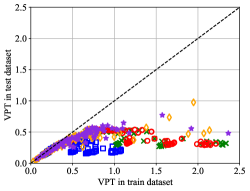
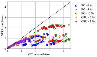
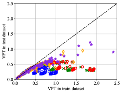
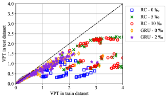
Appendix C Dimensionality Reduction with Singular Value Decomposition
Singular Value Decomposition (SVD) can be utilized to perform dimensionality reduction in a dataset by identifying the modes that capture the highest variance in the data and then performing a projection on these modes. Assuming that a data matrix is given by stacking the time-evolution of a state as , where the index is the number of data samples. By subtracting the temporal mean and stacking the data, we end up with the data matrix . Performing SVD on leads to
| (16) |
with diagonal, with descending diagonal elements. The columns of matrix are considered the modes of the SVD, while the square singular values of correspond to the data variance explained by these modes. This variance is also referred to as energy. In order to calculate the percentage of the total energy the square of the singular value of each mode has to be divided by the sum of squares of the singular values of all modes. In order to reduce the dimensionality of the dataset, we first have to decide on the reduced order dimension . Then we identify the eigenvectors corresponding to the most high-energetic eigenmodes. These are given by the first columns of , i.e., . We discard the low-energetic modes . The dimension of the truncated eigenvector matrix is . In order to reduce the dimensionality of the dataset, each vector is projected to by
| (17) |
In the Lorenz-96 system, we construct a reduced order observable with modes of the system. The cumulative energy distribution along with a contour plot of the state and the mode evolution is illustrated in Figure 18.
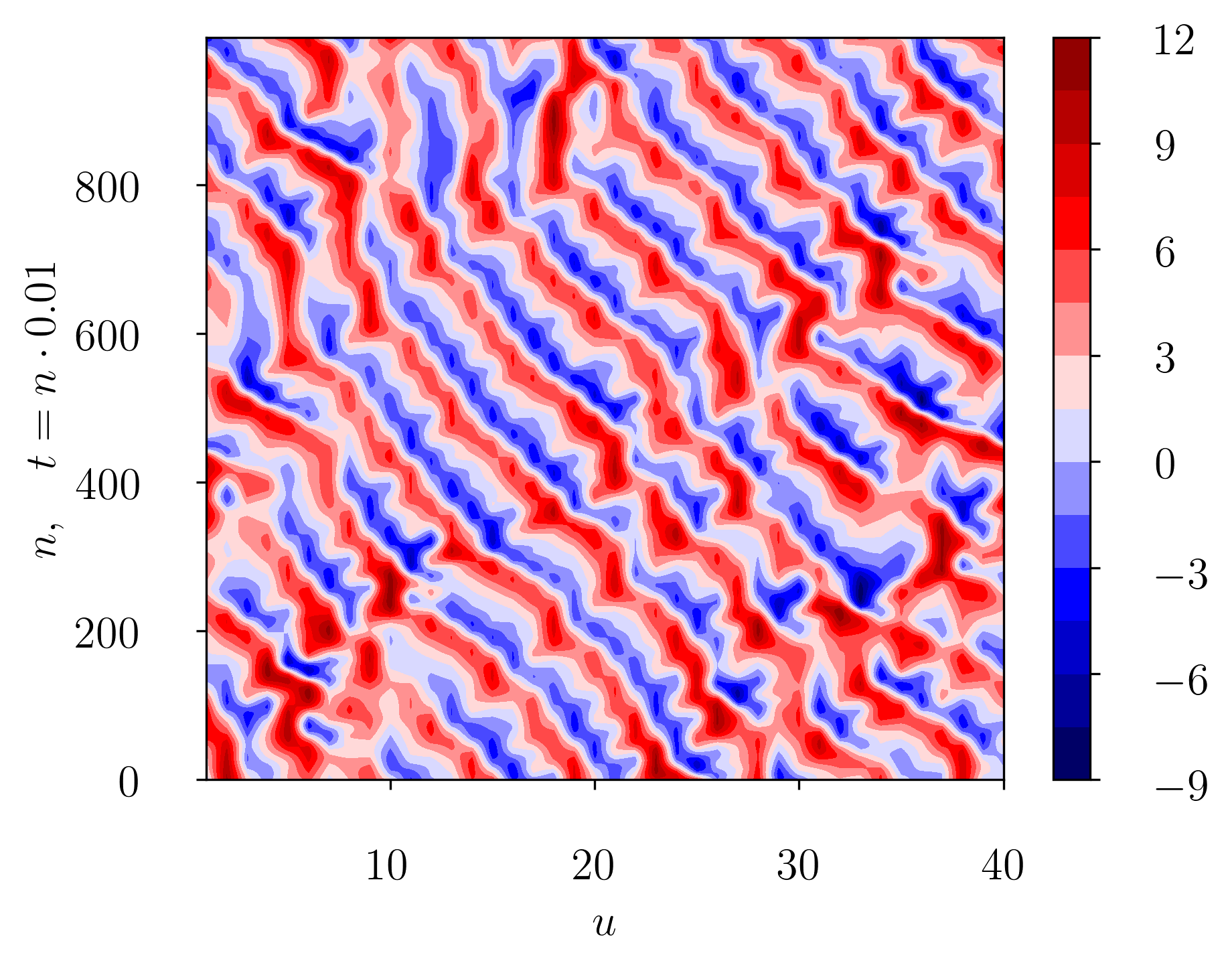
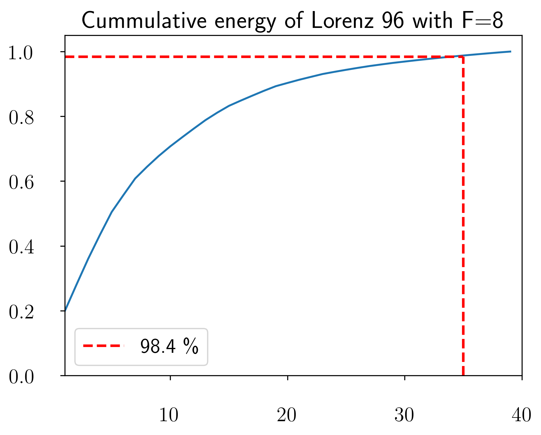
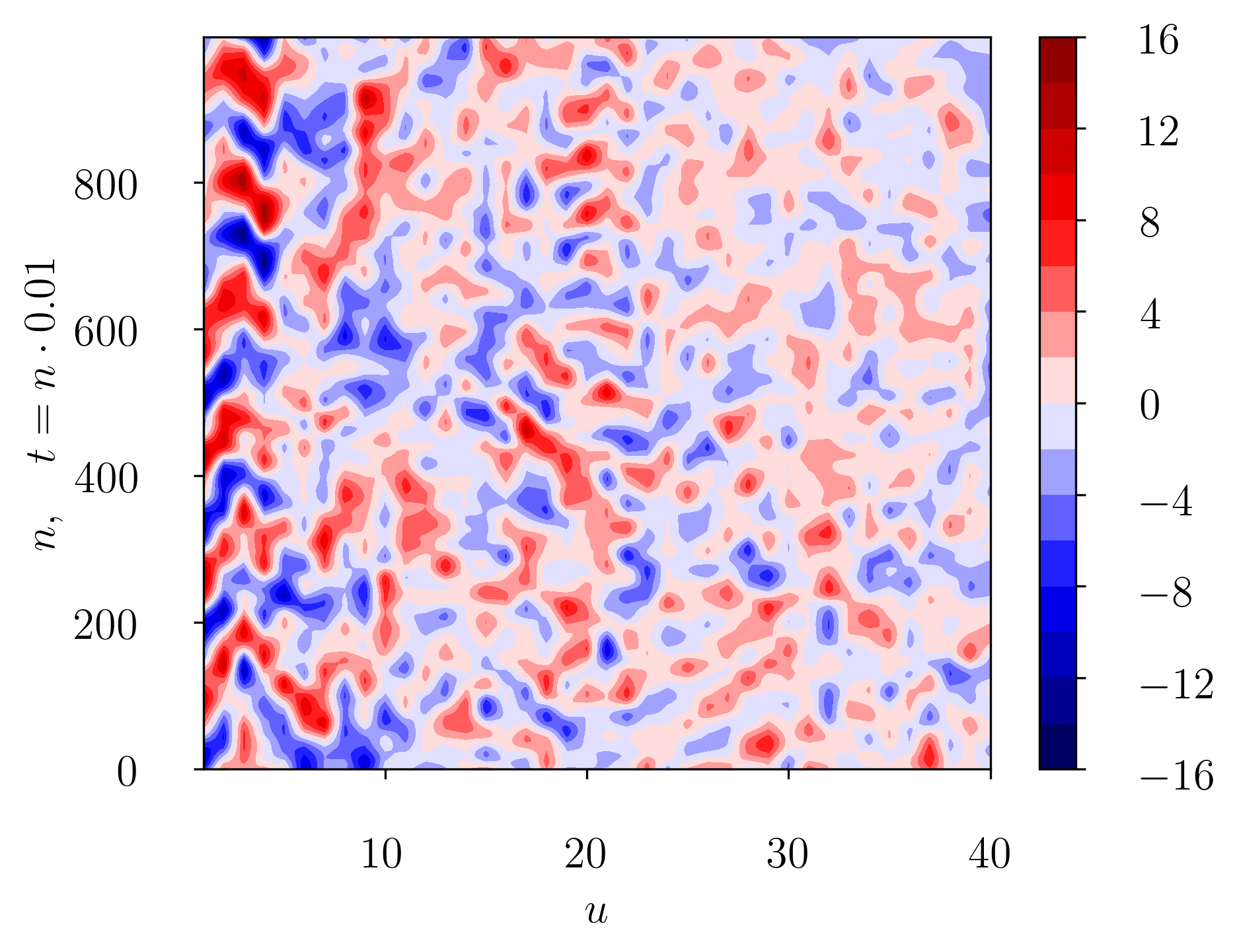
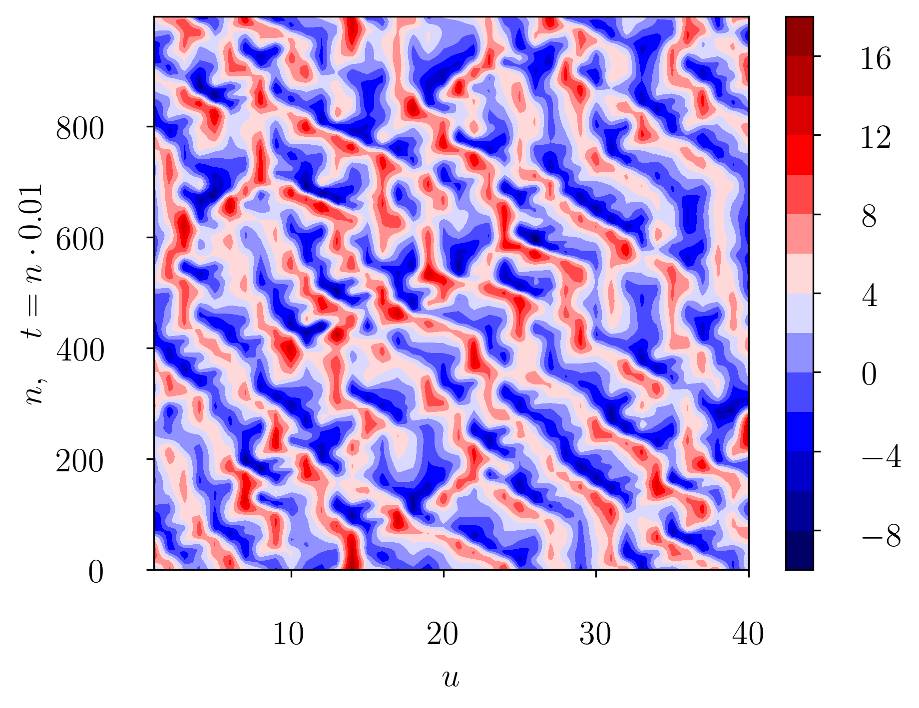
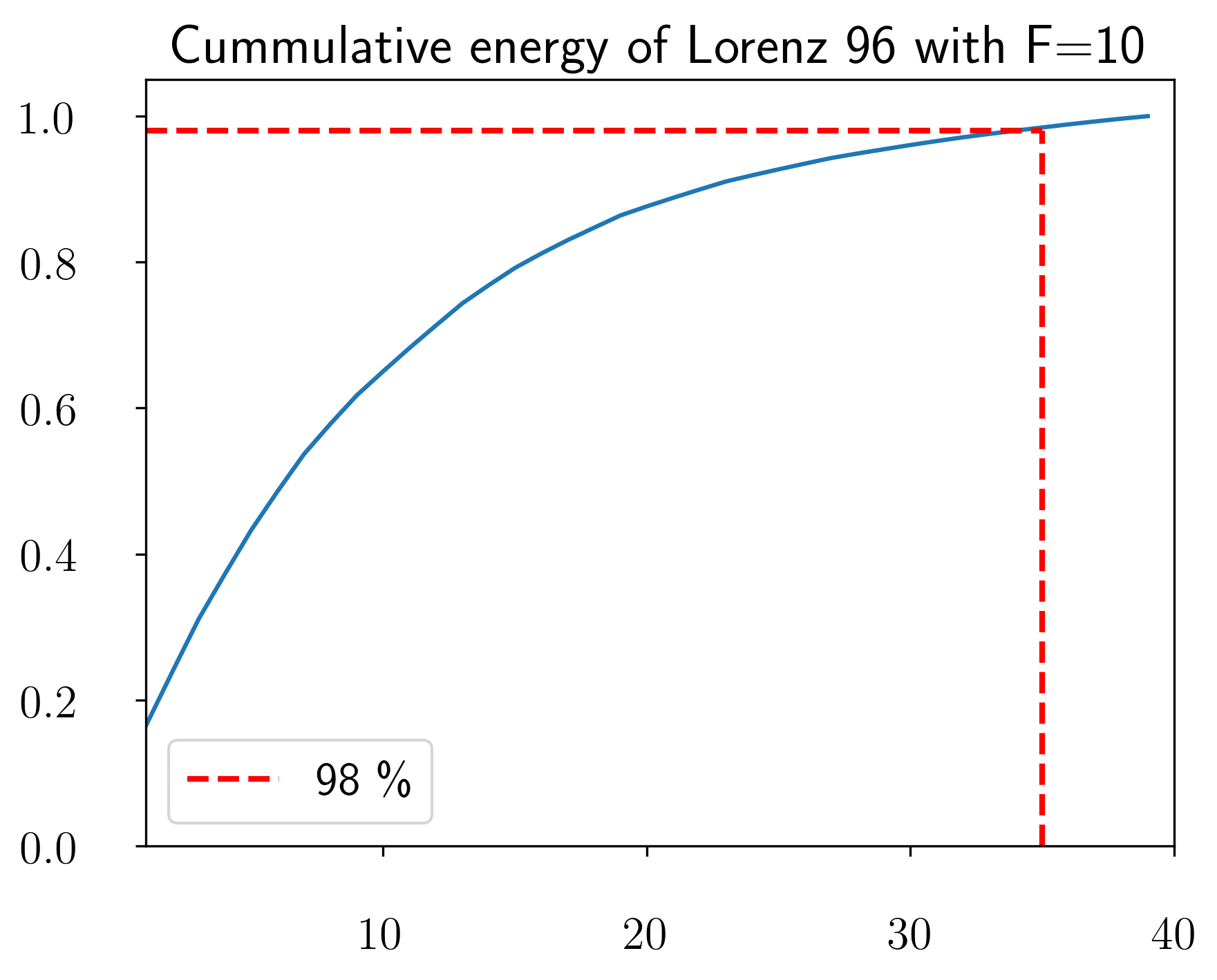
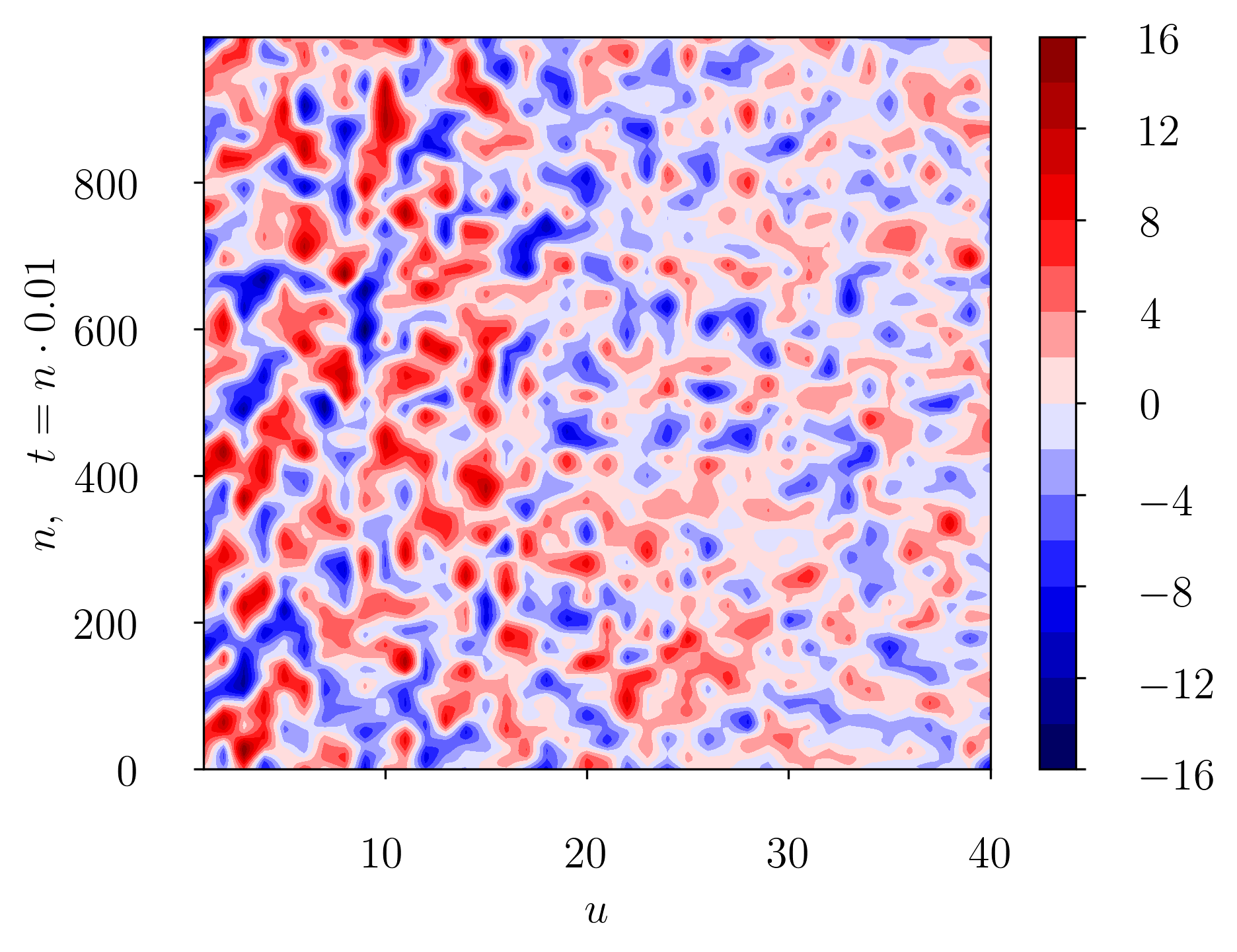
Appendix D Calculation of Lyapunov Spectrum
The true Lyapunov exponents of the KS equation are computed as in (Pathak et al., 2018a) by solving the KS equations in the Fourier space with a fourth order time-stepping method called ETDRK4 (Kassam and Trefethen, 2005) and utilizing a QR decomposition approach. The trained RNN model with GRU cell is used as a surrogate to compute the full Lyapunov spectrum of the Kuramoto-Sivashinsky system. Recall that the RNN dynamics are given by
| (18) | ||||
where is the hidden-to-hidden and is the hidden-to-output mapping, is an observable of the state, and is the hidden state of the RNN. All models utilized in this work share this common architecture. They only differ in the forms of and . More importantly, the output mapping is linear, i.e.,
| (19) |
The LEs are calculated based on the Jacobian of the hidden state dynamics along the trajectory. In the following we compute the Jacobian using Equation 18. By writing down the equations for two consecutive time-steps, we get
| Timestep : | (20) | |||
| (21) | ||||
| Timestep : | (22) |
The partial Jacobians needed to compute the total Jacobian are:
| (23) | |||
| (24) | |||
| (25) |
In total we can write:
| (26) | |||
| (27) | |||
| (28) |
A product of this Jacobian along the orbit is developed and iteratively orthonormalized every steps using the Gram-Schmidt method to avoid numerical divergence and keep the columns of the matrix independent. We check the convergence criterion by tracking the estimated LE values every time-steps. The input provided to the algorithm is a short time-series of length to initialize the RNN and warm-up the hidden state (where the tilde denotes experimental or simulation data), the length of this warm-up time-series , the number of the LE to calculate , the maximum time to unroll the RNN , a normalization time and an additional threshold used as an additional termination criterion. The function computes the sum of each column of a matrix, i.e., . This method can be applied directly to RNNs with one hidden state like RC or GRUs. An adaptation to the LSTM is left for future research. The pseudocode of the algorithm to calculate the Lyapunov exponents of the RNN is given in Algorithm 1.
Appendix E Model Hyperparameters
For the Lorenz-96 system space with (in the PCA mode), we used the hyperparameters reported on Table 2 for RC and Table 3 for GRU/LSTM models. For the parallel architectures in the state space of Lorenz-96 the hyperparameters are reported on Table 5 and Table 6 for the parallel RC and GRU/LSTM models respectively. For the parallel architectures in the state space of the Kuramoto-Sivashinsky architecture the hyperparameters are reported on Table 7 and Table 8 for the parallel RC and GRU/LSTM models respectively. We note here that in all RNN methods, the optimizer used to update the network can also be optimized. To alleviate the computational burden we stick to Adam.
| Hyperparameter | Explanation | Values |
| reservoir size | ||
| training data samples | ||
| Solver | Pseudoinverse/LSQR/Gradient descent | |
| degree of | ||
| radius of | ||
| input scaling | ||
| regularization | ||
| observed state dimension | ||
| warm-up steps (testing) | ||
| noise level in data |
| Hyperparameter | Explanation | Values |
| hidden state size | layers of | |
| training data samples | ||
| batch-size | ||
| BPTT forward time steps | ||
| BPTT truncated backprop. length | ||
| BPTT skip gradient parameter | ||
| initial learning rate | ||
| zoneout probability | ||
| observed state dimension | ||
| warm-up steps (testing) | ||
| noise level in data |
| Hyperparameter | Explanation | Values |
| reservoir size | ||
| number of groups | ||
| group size | ||
| interaction length | ||
| training data samples | ||
| Solver | Pseudoinverse/LSQR/Gradient descent | |
| degree of | ||
| radius of | ||
| input scaling | ||
| regularization | ||
| observed state dimension | ||
| warm-up steps (testing) |
| Hyperparameter | Explanation | Values |
| hidden state size | ||
| number of groups | ||
| group size | ||
| interaction length | ||
| training data samples | ||
| batch-size | ||
| BPTT forward time steps | ||
| BPTT truncated backprop. length | ||
| BPTT skip gradient parameter | ||
| initial learning rate | ||
| zoneout probability | ||
| observed state dimension | ||
| warm-up steps (testing) |
| Hyperparameter | Explanation | Values |
| reservoir size | ||
| number of groups | ||
| group size | ||
| interaction length | ||
| training data samples | ||
| Solver | Pseudoinverse | |
| degree of | ||
| radius of | ||
| input scaling | ||
| regularization | ||
| observed state dimension | ||
| warm-up steps (testing) |
| Hyperparameter | Explanation | Values |
| hidden state size | ||
| number of groups | ||
| group size | ||
| interaction length | ||
| training data samples | ||
| batch-size | ||
| BPTT forward time steps | ||
| BPTT truncated backprop. length | ||
| BPTT skip gradient parameter | ||
| initial learning rate | ||
| zoneout probability | ||
| observed state dimension | ||
| warm-up steps (testing) |
| Hyperparameter | Explanation | Values |
| hidden state size | ||
| number of groups | ||
| group size | ||
| interaction length | ||
| training data samples | ||
| batch-size | ||
| BPTT forward time steps | ||
| BPTT truncated backprop. length | ||
| BPTT skip gradient parameter | ||
| initial learning rate | ||
| zoneout probability | ||
| observed state dimension | ||
| warm-up steps (testing) |
Appendix F Additional Results - Lorenz-96 - Divergence of Unitary and RC RNNs
In this section, we try to quantify the divergence effect due to the accumulation of the forecasting error in the iterative prediction. In Figure 19 we present violin plots with fitted kernel density estimates for the number of divergent predictions of each hyperparameter set, computed based on all tested hyperparameter sets for forcing regimes and observable dimensions . The annotated lines denote the minimum, mean and maximum number of divergent predictions over the 100 initial conditions of all hyperparameter sets. In the fully observable systems , in both forcing regimes , there are many models (hyperparameter sets) with zero divergent predictions for RC, GRU and LSTM, as illustrated by the wide lower part of the violin plot. In contrast, most hyperparameter sets in Unitary networks lead to models whose iterative predictions diverge from the attractor, as illustrated by the wide upper part in the violin plot. In the reduced order scenario, this divergence effect seems to be more prominent in RC and Unitary networks, as indicated by the very thin lower part of their violin plots, for both forcing regimes. In contrast, many hyperparameter sets of GRU and LSTM models lead to stable iterative prediction. This indicates that hyperparameter tuning in RC and Unitary networks when the system state is not fully observed, is cumbersome compared to LSTM and GRU networks. One example of this divergence effect in an initial condition from the test dataset is illustrated in Figure 20. The RC and the Unitary networks diverge in the reduced order state predictions after approximately two Lyapunov times.
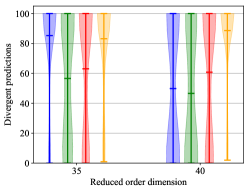
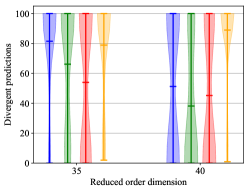
RC ; GRU ; LSTM ; Unit ;
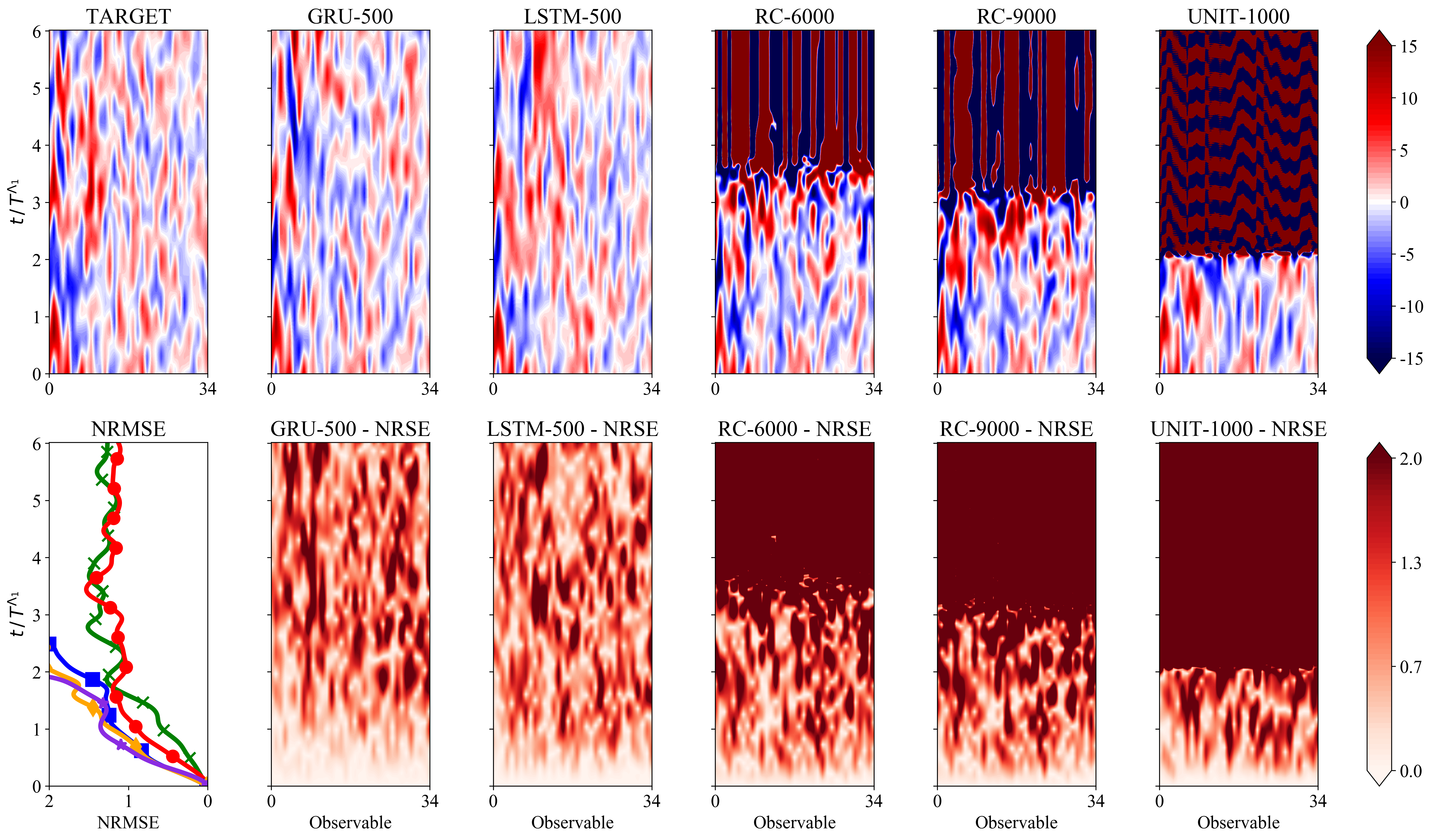
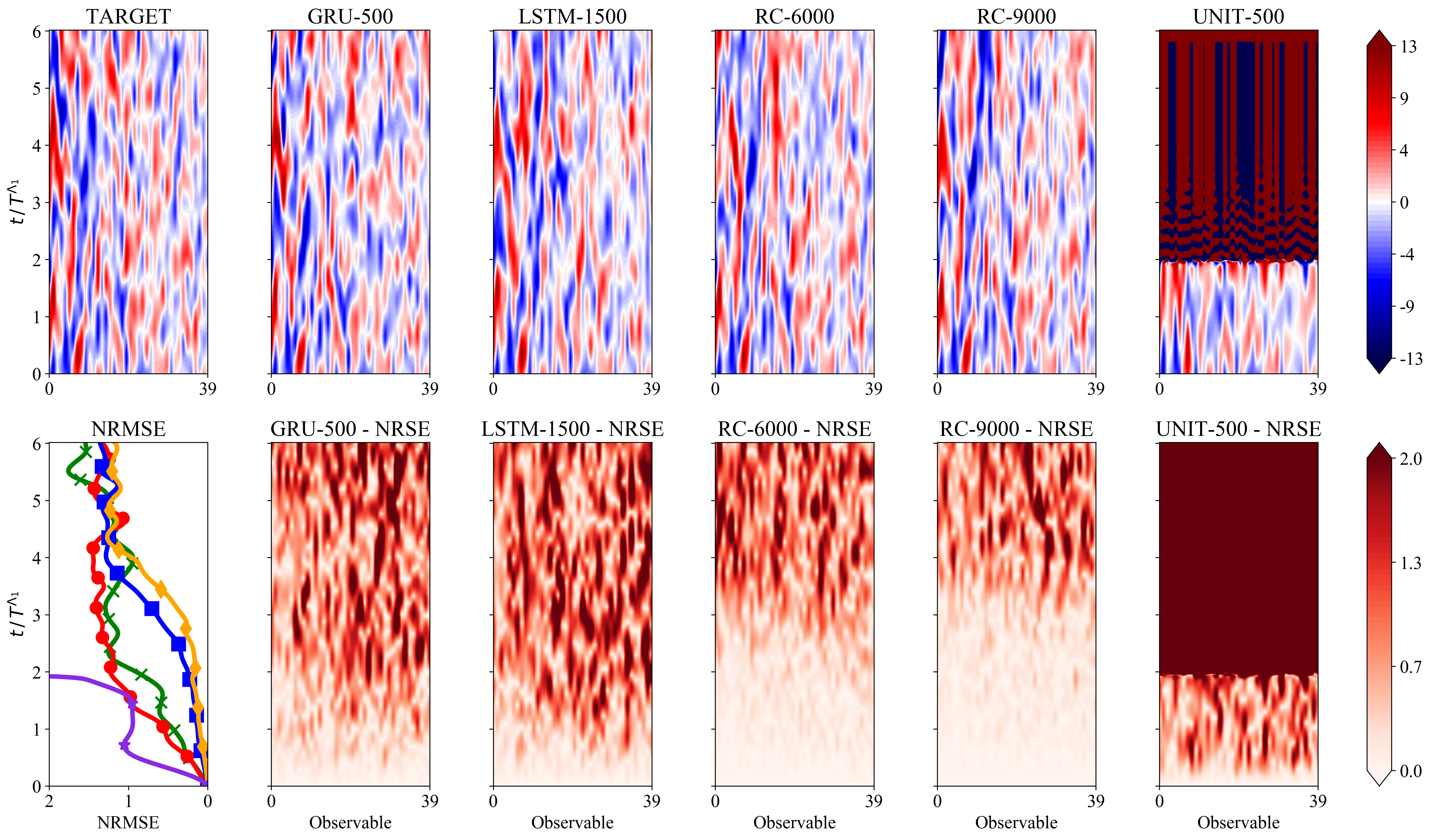
GRU ; LSTM ; RC-6000 ; RC-9000 ; Unit ;
Appendix G Additional Results - Lorenz-96 -
In Figure 21, we provide additional results for the forcing regime that are in agreement with the main conclusions drawn in the main manuscript for the forcing regime . An example of a single forecast of the models starting from an initial condition in the test dataset is given in Figure 22
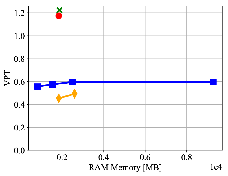
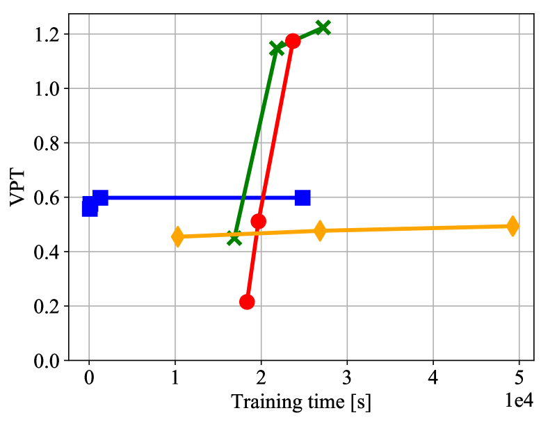
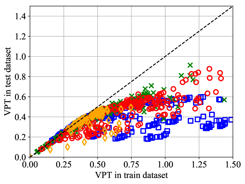
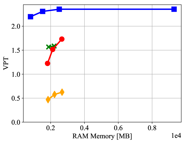
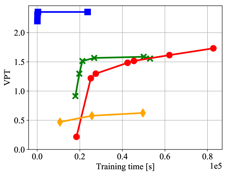
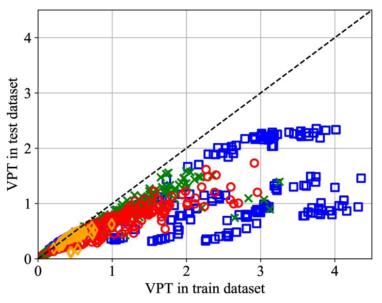
RC ; GRU ; LSTM ; Unit ; Ideal ;
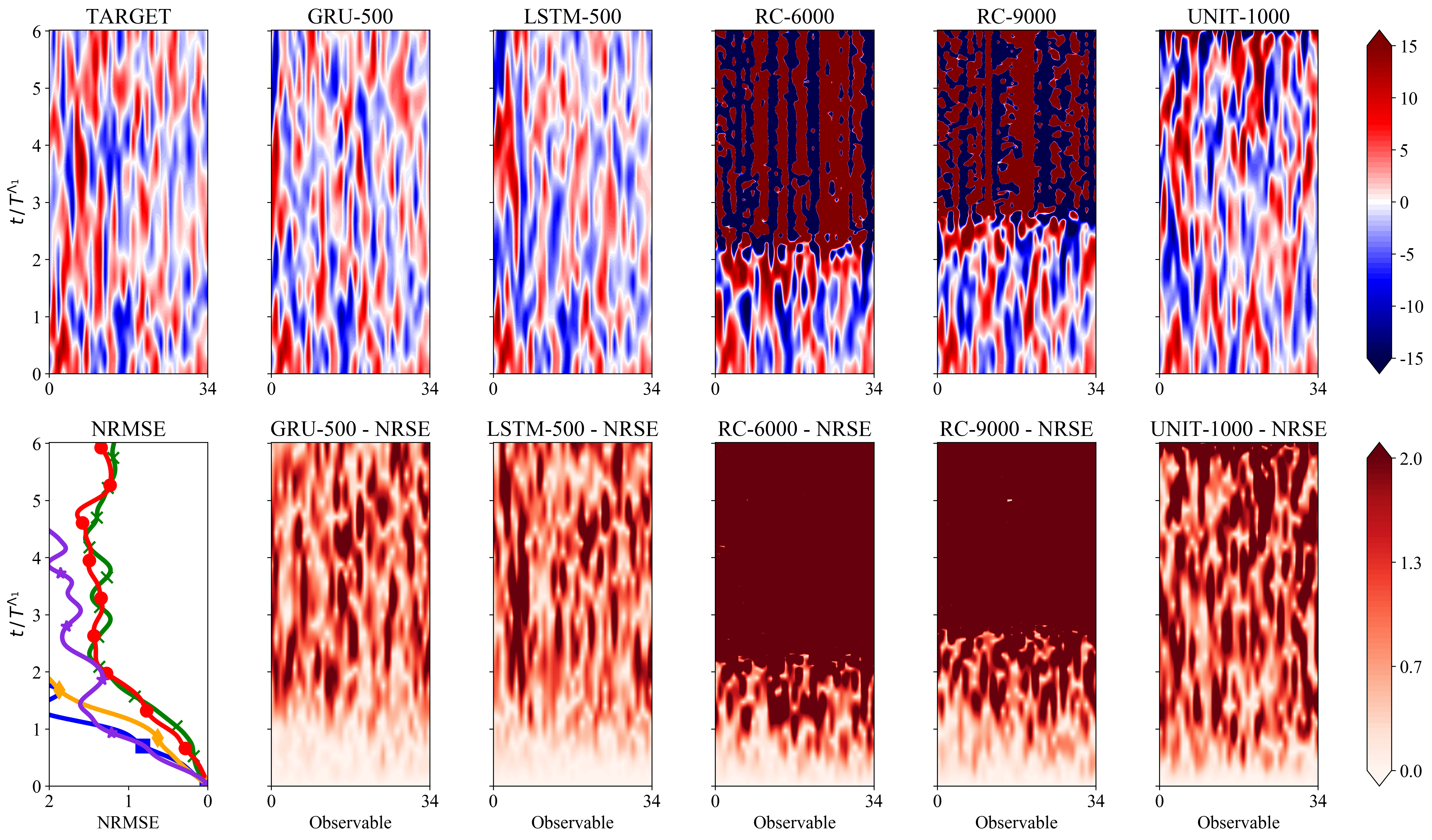
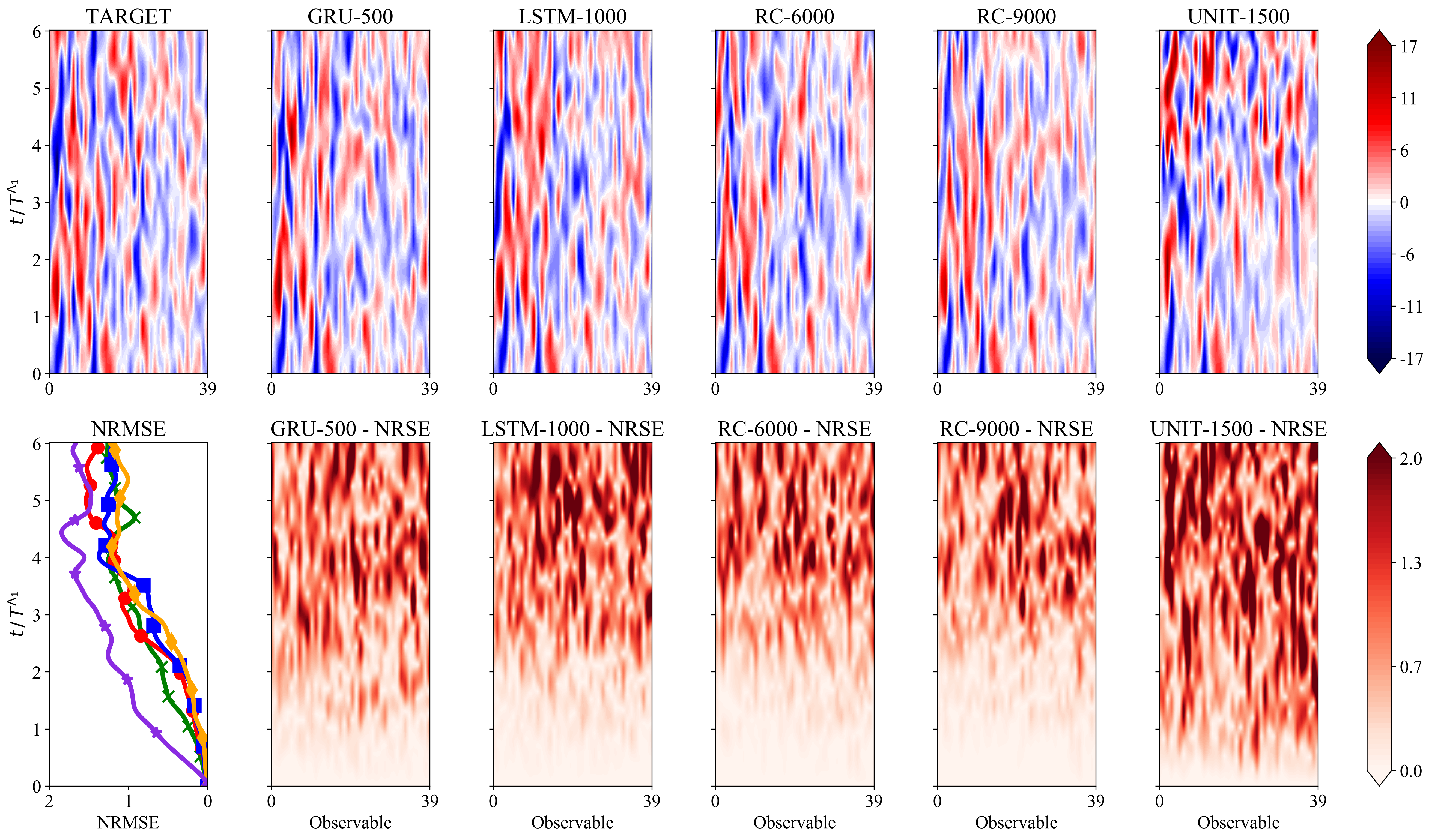
GRU ; LSTM ; RC-6000 ; RC-9000 ; Unit ;
Appendix H Temporal Dependencies and Backpropagation
In our study, in order to train the GRU and LSTM models with back-propagation through time (BPTT), we need to tune the parameters and . The first one denotes the truncated back-propagation length (also referred to as sequence length) and the second the number of future time-steps used to compute the loss and backpropagate the gradient during training at each batch. In the hyperparameter study considered in this work, we varied and .
In Figure 23 we plot the forecasting efficiency of LSTM and GRU models trained with different parameters in terms of the Valid Prediction Time (VPT) in the test dataset (averaged over 100 initial conditions) on the Lorenz-96 system for . In the reduced order scenario case, we observe that models with a large sequence length and a large prediction length are pivotal in order to achieve a high forecasting efficiency. This implies that there are temporal correlations in the data that cannot be easily captured by other models with smaller horizons. In contrast, in the full order scenario, models with smaller perform reasonably well, demonstrating that the need of capturing temporal correlations in the data in order to forecast the evolution is less prominent, since the full information of the state of the system is available.
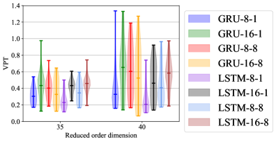
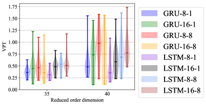
Appendix I Over-fitting of Parallel Models
In this section, we provide results on the overfitting of the models in the parallel setting in the Lorenz-96 model in Figure 24(a) and the Kuramoto-Sivashinsky equation in Figure 24(b). In both cases we do not observe overfitting issues as the predictive performance in terms of the VPT of the models in the test dataset is very close to that in the training dataset, emphasizing that the generalization ability of the models is good.
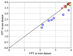
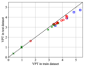
RC ; GRU ; LSTM ;