Improving Gradient Estimation in Evolutionary Strategies With Past Descent Directions
Abstract
Evolutionary Strategies (ES) are known to be an effective black-box optimization technique for deep neural networks when the true gradients cannot be computed, such as in Reinforcement Learning. We continue a recent line of research that uses surrogate gradients to improve the gradient estimation of ES. We propose a novel method to optimally incorporate surrogate gradient information. Our approach, unlike previous work, needs no information about the quality of the surrogate gradients and is always guaranteed to find a descent direction that is better than the surrogate gradient. This allows to iteratively use the previous gradient estimate as surrogate gradient for the current search point. We theoretically prove that this yields fast convergence to the true gradient for linear functions and show under simplifying assumptions that it significantly improves gradient estimates for general functions. Finally, we evaluate our approach empirically on MNIST and reinforcement learning tasks and show that it considerably improves the gradient estimation of ES at no extra computational cost.
1 Introduction
Evolutionary Strategies (ES) [1, 2, 3] are a black-box optimization technique, that estimate the gradient of some objective function with respect to the parameters by evaluating parameter perturbations in random directions. The benefits of using ES in Reinforcement Learning (RL) were exhibited in [4]. ES approaches are highly parallelizable and account for robust learning, while having decent data-efficiency. Moreover, black-box optimization techniques like ES do not require propagation of gradients, are tolerant to long time horizons, and do not suffer from sparse reward distributions [4]. This lead to a successful application of ES in variety of different RL settings [5, 6, 7, 8]. Applications of ES outside RL include for example meta learning [9].
In many scenarios, the true gradient is impossible to compute, however surrogate gradients are available. Here, we use the term surrogate gradients for directions that are correlated but usually not equal to the true gradient, e.g. they might be biased or unbiased approximations of the gradient. Such scenarios include models with discrete stochastic variables [10], learned models in RL like Q-learning [11], truncated backpropagation through time [12] and feedback alignment [13], see [14] for a detailed exhibition. If surrogate gradients are available, it is beneficial to preferentially sample parameter perturbations from the subspace defined by these directions [14]. The proposed algorithm [14] requires knowing in advance the quality of the surrogate gradient, does not always provide a descent direction that is better than the surrogate gradient, and it remains open how to obtain such surrogate gradients in general settings.
In deep learning in general, experimental evidence has established that higher order derivatives are usually "well behaved", in which case gradients of consecutive parameter updates correlate and applying momentum speeds up convergence [15, 16, 17]. These observations suggest that past update directions are promising candidates for surrogate gradients.
In this work, we extend the line of research of [14]. Our contribution is threefold:
-
•
First, we show theoretically how to optimally combine the surrogate gradient directions with random search directions. More precisely, our approach computes the direction of the subspace spanned by the evaluated search directions that is most aligned with the true gradient. Our gradient estimator does not need to know the quality of the surrogate gradients and always provides a descent direction that is more aligned with the true gradient than the surrogate gradient.
-
•
Second, above properties of our gradient estimator allow us to iteratively use the last update direction as a surrogate gradient for our gradient estimator. Repeatedly using the last update direction as a surrogate gradient will aggregate information about the gradient over time and results in improved gradient estimates. In order to demonstrate how the gradient estimate improves over time, we prove fast convergence to the true gradient for linear functions and show, that under simplifying assumptions, it offers an improvement over ES that depends on the Hessian for general functions.
-
•
Third, we validate experimentally that these results transfer to practice, that is, the proposed approach computes more accurate gradients than standard ES. We observe that our algorithm considerably improveŝ gradient estimation on the MNIST task compared to standard ES and that it improves convergence speed and performance on the tested Roboschool reinforcement learning environments.
2 Related Work
Evolutionary strategies [1, 2, 3] are black box optimization techniques that approximate the gradient by sampling finite differences in random directions in parameter space. Promising potential of ES for the optimization of neural networks used for RL was demonstrated in [4]. They showed that ES gives rise to efficient training despite the noisy gradient estimates that are generated from a much smaller number of samples than the dimensionality of parameter space. This placed ES on a prominent spot in the RL tool kit [5, 6, 7, 8].
The history of descent directions was previously used to adapt the search distribution in covariance matrix adaptation ES (CMA-ES) [18]. CMA-ES constructs a second-order model of the underlying objective function and samples search directions and adapts step size according to it. However, maintaining the full covariance matrix makes the algorithm quadratic in the number of parameters, and thus impractical for high-dimensional spaces. Linear time approximations of CMA-ES like diagonal approximations of the covariance matrix [19] often do not work well. E.g. even for linear functions the gradient estimates will not converge to the true gradient, instead the step-size of the descent direction is arbitrarily increased. Our approach differs as we simply improve the gradient estimation and then feed the gradient estimate to a first-order optimization algorithm.
Our work is inspired by the line of research of [14], where surrogate gradient directions are used to improve gradient estimations by ’elongating’ the search space along these directions. That approach has two shortcomings. First, the bias of the surrogate gradients needs to be known to adapt the covariance matrix. Second, once the bias of the surrogate gradient is too small, the algorithm will not find a better descent direction than the surrogate gradient.
Another related area of research investigates how to use momentum for the optimization of deep neural networks. Applying different kinds of momentum has become one of the standard tools in current deep learning and it has been shown to speed-up learning in a very wide range of tasks [20, 16, 17]. This hints, that for many problems the higher-order terms in deep learning models are "well-behaved" and thus, the gradients do not change too drastically after parameter updates. While these approaches use momentum for parameter updates, our approach can be seen as a form of momentum when sampling directions from the search space of ES.
3 Gradient Estimation
We aim at minimizing a function by steepest descent. In scenarios where the gradient does not exist or is inefficient to compute, we are interested in obtaining some estimate of the (smoothed) gradient of that provides a good parameter update direction.
3.1 The ES Gradient Estimator
ES considers the function that is obtained by Gaussian smoothing
where is a parameter modulating the size of the smoothing area and is the -dimensional Gaussian distribution with being the all vector and being the -dimensional identity matrix. The gradient of with respect to parameters is given by
which can be sampled by a Monte Carlo estimator, see [5]. Often antithetic sampling is used, as it reduces variance [5]. The antithetic ES gradient estimator using samples is given by
| (1) |
where are independently sampled from for . This gradient estimator has been shown to be effective in RL settings [4].
3.2 Our One Step Gradient Estimator
We first give some intuition before presenting our gradient estimator formally. Given one surrogate gradient direction , our one step gradient estimator applies the following sampling strategy. First, it estimates how much the gradient points into the direction of by antithetically evaluating in the direction of . Second, it estimates the part of that is orthogonal to by evaluating random, pairwise orthogonal search directions that are orthogonal to . In this way, our estimator detects the optimal lengths of the parameter update step into the both surrogate direction and the evaluated orthogonal directions (e.g. if and are parallel, the update step is parallel to , and if they are orthogonal the step into direction has length ). Additionally, if the surrogate direction and the gradient are not perfectly aligned, then the gradient estimate almost surely improves over the surrogate direction due to the contribution from the evaluated directions orthogonal to . In the following we define our estimator formally and prove that the estimated direction possesses best possible alignment with the gradient that can be achieved with our sampling scheme.
We assume that pairwise orthogonal surrogate gradient directions are given to our estimator. Denote by the subspace of that is spanned by the , and by the subspace that is orthogonal to . Further, for vectors and , we denote by and the normalized vector and , respectively. Let be random orthogonal unit vectors from . Then, our estimator is defined as
| (2) |
We write , where and are the projections of on and , respectively. In essence, the first sum in (2) computes by assessing the quality of each surrogate gradient direction, and the second sum estimates similar to an orthogonalized antithetic ES gradient estimator, that samples directions from , see [5]. We remark that we require pairwise orthogonal unit directions for the optimality proof. Due to the orthogonality of the directions, no normalization factor like the factor in (1) is required in (2). In practice, the dimensionality is often much larger than . Then, sampling pairwise orthogonal unit vecotrs is nearly identical to sampling the s from a distribution, because in high-dimensional space the norm of is highly concentrated around and the cosine of two such random vectors is highly concentrated around .
For the sake of analysis, we assume that is differentiable and we assume equality for the following first order approximation
In the following, we will omit the in . Our first proposition states that computes the direction in the subspace spanned by that is most aligned with .
Proposition 1 (Optimality of ).
Let be pairwise orthogonal vectors in . Then, computes the projection of on the subspace spanned by . Especially, is the vector of that subspace that maximizes the cosine between and . Moreover, the squared cosine between and is given by
| (3) |
We remark that when evaluating for arbitrary directions , no information about search directions orthogonal to the subspace spanned by the s is obtained. Therefore, one can only hope for finding the best approximation of lying within the subspace spanned by the s, which is accomplished by . The proof of Proposition 1 follows easily from the Cauchy-Schwarz inequality and is given in the appendix.
3.3 Iterative Gradient Estimation Using Past Descent Directions
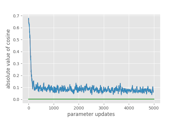
Our gradient estimation algorithm iteratively applies the one step gradient estimator by using the gradient estimate of the last time step as surrogate direction for the current time step. At any time step, our one step gradient estimator provides a better gradient estimate than the surrogate direction. Therefore, the algorithm accumulates information about the gradient, and the gradient estimate becomes more aligned with the true gradient over time. Our algorithm relies on the assumption that gradients are correlated from one time step to the next. This assumption is justified since it is one of the reasons momentum-based optimizers [15, 16, 17] are successful in deep learning. We also explicitly test this assumption experimentally, see Figure 1(a). In the following, we first analyse how fast our algorithm accumulates information about the gradient over time if the gradient is constant, i.e. if a linear function is optimized. In this setting, we show that our algorithm is close to optimal, i.e. the convergence rate is only by a small constant factor smaller than the one of optimal orthogonal sampling, see Theorem 1. Second, we analyse the quality of our gradient estimates for general, non-linear functions, where the gradient changes over time. We show under some simplifying assumptions that, also in the general case, our algorithm builds up an improved gradient estimate over time, see Theorem 2.
We first need some notation. Denote by the search point, by the gradient and by the parameter update step at time , that is, . The iterative gradient estimation algorithm obtains the gradient estimate by computing with the last update direction as surrogate gradient and new random directions . Formally, let be pairwise orthogonal unit directions chosen uniformly from the unit sphere, that is, they are conditioned to be pairwise orthogonal and are marginally uniformly distributed. By defining , and setting , we obtain
| (4) |
Then, Equation 3 of Proposition 1 turns into
| (5) |
The next theorem quantifies how fast the cosine between and converges to , if does not change over time.
Theorem 1 (Convergence rate for linear functions).
Let be iteratively computed using the past update direction and pairwise orthogonal random directions, see Equation (4), and let be the random variable that denotes the cosine between and at time . Then, the expected drift of is . Moreover, let and define to be the first point in time with . It holds
The first bound is tight for close to and follows by an additive drift theorem, while the second bound is tight for close to and follows by a variable drift theorem, see appendix. We remark that an optimal orthogonal gradient estimator requires samples in order to reach a cosine squared of . Since our algorithm evaluates directions per time step, it requires approximately times more samples to reach the same alignment.
Naturally, the linear case is not the most interesting one. However, it is hard to rigorously analyse the case of general , because it is unpredictable how the gradient differs from . Note that , where is the Hessian matrix of at . We define and write where is orthogonal to and has squared norm . Then, the first term of (5) is equal to
In the following, we assume that is a direction orthogonal to chosen uniformly at random. Though, this assumption is not entirely true, it allows to get a grasp on the approximate cosine that our estimator is going to converge to.
Theorem 2.
Let be iteratively computed using the past update direction and pairwise orthogonal random directions, see Equation (4), and let be the random variable that denotes the cosine between and at time . Further, let and assume that , where is a random vector orthogonal to with norm . Choose according to Equation (4) and define to be the cosine between and . Then,
The last theorem implies that the evolution of the cosine depends heavily on the cosine between consecutive gradients. Let . Then, the theorem implies that the drift is positive if and negative otherwise. Thus, if would not change over time, we would expect to converge to .
4 Experiments
In this section, we will empirically evaluate the performance of our gradient estimation scheme when combined with deep neural networks. In Section 4.1, we show that it significantly improves gradient estimation for digit classifiers on MNIST. In Section 4.2, we suggest how to overcome issues that arise from function evaluation noise. Finally, in Section 4.3, we evaluate our gradient estimation scheme on RL environments and investigate further issues arising in this setting.
4.1 Gradient Estimation and Performance on MNIST
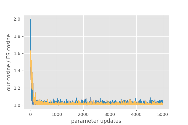
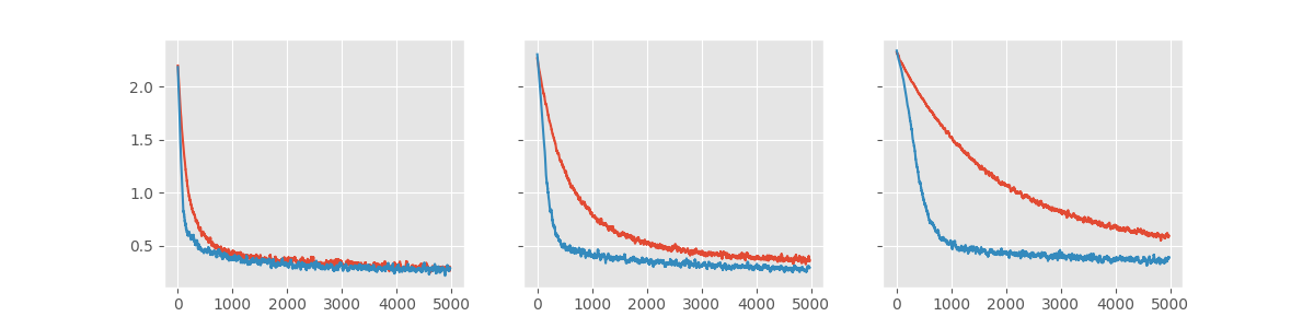
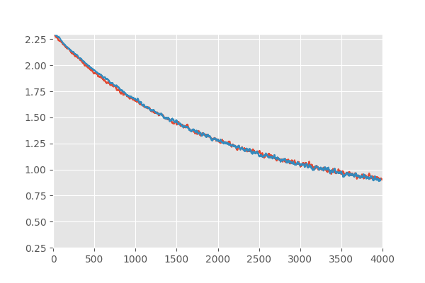
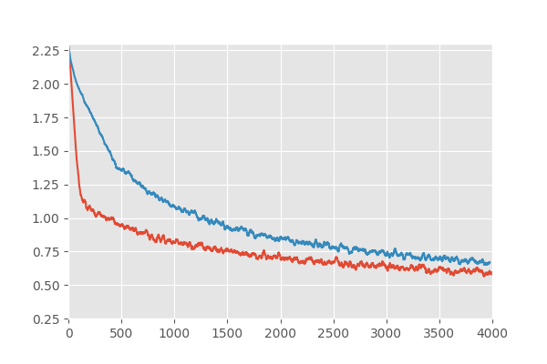
We observe that our approach significantly improves gradient estimation compared to standard ES. Figure 1(a) shows that the key requisite of our iterative gradient estimation scheme is satisfied during training on MNIST, that is, that gradients between consecutive parameter update steps are correlated. Figure 1(b) shows that our approach improves gradient estimation compared to ES during the whole training process and strongly improves it in the beginning of training, where consecutive gradients are most correlated, see Figure 1(a). We observe that our approach strongly outperforms ES in convergence speed and reaches better final performance for all hyperparameters we tested, see Figure 2 and Table 1.
Implementation details: For these experiments, we used a fully connected neural network with two hidden layers with a non-linearity and units each, to have a high dimensional model ( million parameters) . For standard ES random search directions are evaluated at each step. For our algorithm the previous gradient estimate and random search directions are evaluated. We evaluated all directions on the same batch of images in order eliminate function evaluation noise and we resampled after every update step. We used small parameter perturbations (). This is possible because no function evaluation noise is present and because the objective function is already differentiable and therefore no smoothing is required. We test both SGD and Adam optimizers with learning rates in the range .
| Optimizer | Steps until loss | Best loss |
|---|---|---|
| ES + Adam | 433 | 0.242 |
| Ours + Adam | 182 | 0.216 |
| ES + SGD | 727 | 0.305 |
| Ours + SGD | 295 | 0.278 |
4.2 Robustness to Function Evaluation Noise
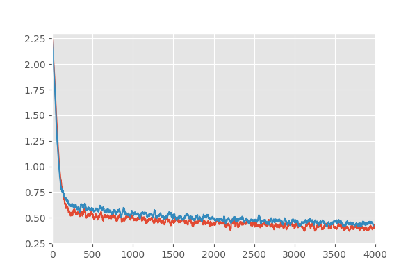
In practice, our iterative gradient estimation scheme may suffer from function evaluation noise because it builds up good gradient estimates over several parameter update steps. Suppose that the past update direction is a good descent direction but it performs poorly on the current batch used for evaluation due to randomness in the batch selection or network evaluation process. Then, this direction is weighted lightly when computing the new update direction, see Equation 4, and therefore the information about this direction will be discarded. We empirically show, that our approach suffers heavily from this issue when artificially injecting noise in the function evaluation process, see Figure 3(b) . Figure 3(c) shows, that this issue can be resolved by using the last update directions for our gradient estimator (see Equation 2). In this case, a good direction is only discarded, when it performs poorly in consecutive evaluation steps, which is very unlikely. We remark that the magnitude of the parameter updates naturally limits , because the -th last update direction is only useful if it is still correlated with the current gradient. Concretely, we found that using the last parameters updates was extremely helpful for smaller learning rates, even in the absence of noise (see Figure 3(c)). However, it did not offer an advantage for larger learning rates.
4.3 Robotic RL environments
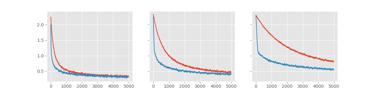
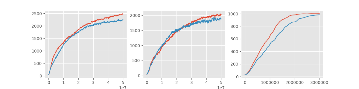
For the next set of experiments, we evaluate our algorithm on three robotics tasks of the Roboschool environment: RoboschoolInvertedPendulum-v1, RoboschoolHalfCheetah-v1 and RoboschoolAnt-v1. Our approach outperforms ES in the pendulum task, and offers a small improvement over ES in the other two tasks, see Figure 4. The improvement of our approach over standard ES is smaller on RL tasks than on the MNIST task. Therefore, we first empirically confirmed that past updated direction are also in RL correlated with the gradient. To test this, we kept track of the average difference between random perturbations and the direction given by our algorithm, after normalizing the rewards. We found that, the direction of our algorithm had an average weight of versus the of a random direction.
RL robotics tasks bring two additional major challenges compared to the MNIST task. First, exploration is crucial to escape local optima and find new solutions, and second, the function evaluation noise is huge due to each perturbation being tested only on a single trajectory. Our proposed solution of robustness against function evaluation noise intertwines with the exploration issue. A rather small step size is necessary in order to use more past directions as surrogate gradients. However, exploration in ES is driven by large perturbation sizes and noisy optimization trajectories. We did not observe improvements when combining the approach of using several past directions with standard hyperparameter settings. We believe that an exhaustive empirical study can shed light onto the effect of our approach on exploration and may further improve the performance on RL tasks. However, running extensive experiments for complex RL environment is computationally expensive.
Implementation details: We use most of the hyper-parameters from the OpenAI implementation 111https://github.com/openai/evolution-strategies-starter . That is, two hidden layers of units each and with a non-linearity. Further, we use a learning rate of , a perturbation standard deviation of and the Adam optimizer, and we also apply fitness shaping [19]. For standard ES random perturbations are evaluated at each step. For our algorithm the previous gradient estimate and random perturbations are evaluated. For the Ant and Cheetah environments, we observed with this setup, that agents often get stuck in a local optima where they stay completely still, instead of running forward. As this happens for both, ES and our algorithm, we tweaked the environments in order to ensure that a true solution to the task is learned and not some some degenerate optima, we tweaked the environments in the following way. We remove the penalty for using electricity and finish the episode if the agent does not make any progress in a given amount of time. In this way, agents consistently escape the local minima. We use a non-linearity on the output of the network, which increased stability of training, as otherwise the output of the network would become very large without an electricity penalty.
5 Conclusion
We proposed a gradient estimator that optimally incorporates surrogate gradient directions and random search directions, in the sense that it determines the direction with maximal cosine to the true gradient from the subspace of evaluated directions. Such a method has many applications as elucidated in [14]. Importantly, our estimator does not require information about the quality of surrogate directions, which allows us to iteratively use past update directions as surrogate directions for our gradient estimator. We theoretically quantified the benefits of the proposed iterative gradient estimation scheme. Finally, we showed that our approach in combination with deep neural networks considerably improves the gradient estimation capabilities of ES, at no extra computational cost. The results on MNIST indicate that the speed of the Evolutionary Strategies themselves, a key part in the current Reinforcement Learning toolbox, is greatly improved. Within Reinforcement Learning an out of the box application of our algorithm yields some improvements. The smaller improvement in RL compared to MNIST is likely due to the interaction of our approach and exploration that is essential in RL. We leave it to future work to explicitly add and study appropriate exploration strategies which might unlock the true potential of our approach in RL.
References
- [1] Ingo Rechenberg. Evolution strategy: Optimization of technical systems by means of biological evolution. Fromman-Holzboog, Stuttgart, 104:15–16, 1973.
- [2] Hans-Paul Schwefel. Evolutionsstrategien für die numerische optimierung. In Numerische Optimierung von Computer-Modellen mittels der Evolutionsstrategie, pages 123–176. Springer, 1977.
- [3] Yurii Nesterov and Vladimir Spokoiny. Random gradient-free minimization of convex functions. Foundations of Computational Mathematics, 17(2):527–566, 2017.
- [4] Tim Salimans, Jonathan Ho, Xi Chen, Szymon Sidor, and Ilya Sutskever. Evolution strategies as a scalable alternative to reinforcement learning. arXiv preprint arXiv:1703.03864, 2017.
- [5] Krzysztof Choromanski, Mark Rowland, Vikas Sindhwani, Richard E Turner, and Adrian Weller. Structured evolution with compact architectures for scalable policy optimization. arXiv preprint arXiv:1804.02395, 2018.
- [6] Xiaodong Cui, Wei Zhang, Zoltán Tüske, and Michael Picheny. Evolutionary stochastic gradient descent for optimization of deep neural networks. In Advances in neural information processing systems, pages 6048–6058, 2018.
- [7] Rein Houthooft, Yuhua Chen, Phillip Isola, Bradly Stadie, Filip Wolski, OpenAI Jonathan Ho, and Pieter Abbeel. Evolved policy gradients. In Advances in Neural Information Processing Systems, pages 5400–5409, 2018.
- [8] David Ha and Jürgen Schmidhuber. Recurrent world models facilitate policy evolution. In Advances in Neural Information Processing Systems, pages 2450–2462, 2018.
- [9] Luke Metz, Niru Maheswaranathan, Jeremy Nixon, Daniel Freeman, and Jascha Sohl-dickstein. Learned optimizers that outperform on wall-clock and validation loss. 2018.
- [10] Yoshua Bengio, Nicholas Léonard, and Aaron Courville. Estimating or propagating gradients through stochastic neurons for conditional computation. arXiv preprint arXiv:1308.3432, 2013.
- [11] Christopher JCH Watkins and Peter Dayan. Q-learning. Machine learning, 8(3-4):279–292, 1992.
- [12] David E Rumelhart, Geoffrey E Hinton, and Ronald J Williams. Learning internal representations by error propagation. Technical report, California Univ San Diego La Jolla Inst for Cognitive Science, 1985.
- [13] Timothy P Lillicrap, Daniel Cownden, Douglas B Tweed, and Colin J Akerman. Random feedback weights support learning in deep neural networks. arXiv preprint arXiv:1411.0247, 2014.
- [14] Niru Maheswaranathan, Luke Metz, George Tucker, Dami Choi, and Jascha Sohl-Dickstein. Guided evolutionary strategies: augmenting random search with surrogate gradients. In International Conference on Machine Learning, pages 4264–4273, 2019.
- [15] Timothy Dozat. Incorporating nesterov momentum into adam. 2016.
- [16] Ilya Sutskever, James Martens, George Dahl, and Geoffrey Hinton. On the importance of initialization and momentum in deep learning. In International conference on machine learning, pages 1139–1147, 2013.
- [17] Sebastian Ruder. An overview of gradient descent optimization algorithms. arXiv preprint arXiv:1609.04747, 2016.
- [18] Nikolaus Hansen. The cma evolution strategy: A tutorial. arXiv preprint arXiv:1604.00772, 2016.
- [19] Daan Wierstra, Tom Schaul, Tobias Glasmachers, Yi Sun, Jan Peters, and Jürgen Schmidhuber. Natural evolution strategies. The Journal of Machine Learning Research, 15(1):949–980, 2014.
- [20] Diederik P Kingma and Jimmy Ba. Adam: A method for stochastic optimization. arXiv preprint arXiv:1412.6980, 2014.
- [21] Johannes Lengler and Angelika Steger. Drift analysis and evolutionary algorithms revisited. Combinatorics, Probability and Computing, 27(4):643–666, 2018.
Appendix A Proof of Theorems
In this Section we prove the theorems from the main paper rigorously.
A.1 Proof of Proposition 1
Note that for this theorem there is no distinction between the directions and . For ease of notation, we denote by . The theorem is a simple application of the Cauchy-Schwarz inequality. Denote by the projection of on the subspace spanned by the s, and let be a vector in that subspace. Then, the Cauchy-Schwarz inequality implies
| (6) |
Equality holds if and only if and have the same direction, which is equivalent to for some . In particular, in this case the cosine squared between and is
| (7) |
∎
A.2 Expectation of Cosine Squared of Random Vectors from the Unit Sphere
Proposition 2.
Let be an -dimensional unit vector, and let be pairwise orthogonal vectors sampled uniformly from the -dimensional unit sphere, that is, they are marginally uniformly distributed and conditioned to be pairwise orthogonal. Then, the expected cosine squared of and is
Proof.
Note that
Denote by the -dimensional unit sphere. Linearity of expectation implies that
By rotational invariance of the unit sphere, we can replace by and obtain
∎
A.3 Proof of Theorem 1
In order to prove Theorem 2, use Equation 5 to compute how depends on . Then, we apply a variable transformation to in order to be able to apply the additive and variable drift theorems from [21], which are stated in Section B.
We can split the normalized gradient into an orthogonal to part and a parallel to part. It holds and since is a unit vector orthogonal to . Recall that , then
| (8) |
and therefore by Equation 5
| (9) |
Define the random process . It holds
| (10) | |||
| (11) |
where we used Proposition 2 in the dimensional subspace that is orthogonal to .
In order to derive the first bound on , we bound the drift of for .
A.4 Proof of Theorem 2
In order to prove the theorem, we need to understand how depends on the value of . It holds . As in Equation 11, we can write , and note that because is a random direction orthogonal to . This implies that
| (13) |
To understand how the evolves we need to analyze how relates to . To that end, we set and write where is orthogonal to and has norm . Then,
Appendix B Drift Theorems
Theorem 3 (Additive Drift, Theorem from [21]).
Let be a Markov chain with state space and assume . Let be the earliest point in time such that . If there exists such that for all , and for all we have
Then,
Theorem 4.
Variable Drift, Theorem from [21]] Let be a Markov chain with state space and with . Let be the earliest point in time such that . Suppose furthermore that there is a positive, increasing function such that for all , we have for all
Then,