Finite element approximation of Lyapunov equations related to parabolic stochastic PDEs

Abstract.

A numerical analysis for the fully discrete approximation of an operator Lyapunov equation related to linear SPDEs (stochastic partial differential equations) driven by multiplicative noise is considered. The discretization of the Lyapunov equation in space is given by finite elements and in time by a semiimplicit Euler scheme. The main result is the derivation of the rate of convergence in operator norm. Moreover, it is shown that the solution of the equation provides a representation of a quadratic and path dependent functional of the SPDE solution. This fact yields a deterministic numerical method to compute such functionals. As a secondary result, weak error rates are established for a fully discrete finite element approximation of the SPDE with respect to this functional. This is obtained as a consequence of the approximation analysis of the Lyapunov equation. It is the first weak convergence analysis for fully discrete finite element approximations of SPDEs driven by multiplicative noise that obtains double the strong rate of convergence, especially for path dependent functionals and smooth spatial noise. Numerical experiments illustrate the results empirically and it is demonstrated that the deterministic method has advantages over Monte Carlo sampling in a stability context.

1. Introduction

Lyapunov and Riccati equations have been studied for linear quadratic control and filtering of stochastic partial differential equations (SPDEs for short) since the late 1970s (see references below). Riccati equations are operator equations containing a nonlinear quadratic term. Their solutions provide optimal feedback controls for stochastic control problems and the covariance operators of the filtering distribution in optimal filtering with the Kalman–Bucy filter (see, e.g., [18] for a Hilbert-space-valued setting with bounded generators and trace-class noise). Removing the quadratic term, linear operator equations called Lyapunov equations are obtained. They are crucial for stability analysis and connected to quadratic functionals of SPDEs driven by multiplicative noise.

In this work we establish a complete error analysis for numerical discretizations of Lyapunov equations by the semiimplicit Euler method in time and a finite element method in space. We connect these approximations to approximations of path dependent quadratic functionals of SPDEs. This connection allows us to show weak convergence rates of the SPDE approximation which are twice the strong rates. Our analysis can be used as a stepping stone for approximation results on Riccati equations in future work.

The two main equations that we connect are the linear parabolic SPDE

(1) $$\mathrm{d}X(t)+AX(t)\,\mathrm{d}t=B(X(t))\,\mathrm{d}W(t)$$

with initial condition $X(0)=X_{0}$ in a Hilbert space $H$ and the operator valued Lyapunov equation, written in variational form,

(2) $$\frac{\mathrm{d}}{\mathrm{d}t}\langle L(t)\phi,\psi\rangle+a(L(t)\phi,\psi)+a(L(t)\psi,\phi)=\langle R\phi,R\psi\rangle+\langle L(t)B(\phi),B(\psi)\rangle_{{\mathcal{L}}_{2}^{0}}$$

with $L(0)=G^{\ast}G$, where ${\mathcal{L}}_{2}^{0}$ refers to a class of Hilbert–Schmidt operators. We show in Section 3 that these are connected via

(3) $$\langle L(T)x,x\rangle=\Phi(x)$$

with respect to the quadratic functional

(4) $$\Phi(x)={\mathbb{E}}\Big{[}\int_{0}^{T}\|RX(t)\|^{2}\,\mathrm{d}t+\|GX(T)\|^{2}\Big{|}X(0)=x\Big{]}.$$

Here $a(\cdot,\cdot)$ denotes the bilinear form corresponding to the operator $-A$ that generates an analytic semigroup and $W$ is a cylindrical Wiener process. This includes the classical case of a $Q$-Wiener process with trace-class covariance. For the complete details on the setting, the reader is referred to Section 2.

We study Lyapunov equations in a new generality suitable for numerical analysis with an emphasis on regularity. It was surprising to us that the literature does not cover the setting of cylindrical noise (cf. [15, 19, 20, 21, 23, 26, 27, 34]). We therefore develop the solution theory for the Lyapunov equation and prove existence and uniqueness by the Banach fixed point theorem and the Gronwall lemma.

To show (3), we use tools from numerical analysis. We approximate both equations (2) and (1) on a finite-dimensional subspace $V_{h}$ such as a finite element space and show that (3) holds in the semidiscrete setting. Convergence establishes equality in the limit and gives as a byproduct convergence to the Lyapunov equation and weak convergence of the SPDE approximation.

For the fully discrete approximation of the Lyapunov equation (2), we discretize the above semidiscrete approximation by a semiimplicit Euler method in time. Results on numerical methods for Lyapunov and Riccati equations for stochastic problems are rare. The results of this paper are most closely related to those of [31], which only considers one-dimensional noise in an abstract approximation framework for Riccati equations. Connected to our problem are also [30], in which a time-independent Lyapunov equation related to an approximation of (1) is employed as part of a bigger problem, and [6], which assumes convergence of an approximation of a Riccati equation to derive strong convergence of a finite element approximation of a controlled version of (1). To the best of our knowledge, this work is the first to provide rigorous a priori convergence rates for a fully discrete numerical approximation of the Lyapunov equation (2) in the infinite-dimensional noise setting and the first to connect such approximations to weak convergence for the related SPDE (1).

Weak convergence of numerical approximations of SPDEs with additive noise is a well understood topic, see, e.g., for implicit Euler in time [36] and for finite element and spectral Galerkin methods in space [3, 8, 14]. For multiplicative noise the literature is still restricted to special cases. Weak rates of convergence have been obtained for discretization in time with implicit [9, 16] and exponential [24] Euler schemes and in space with a spectral Galerkin method [12]. For the finite element method, proofs are restricted to the spatially semidiscrete setting with (essentially) linear multiplicative space-time white noise [3]. The fully discrete setting and more regular noise are still open. One reason for this is the appearance of an extra term [3] which is not present in the spectral Galerkin method [12].

Based on the convergence analysis of the fully discrete approximation of the Lyapunov equation and the connection (3), we are able to extend the existing weak convergence analysis for finite element approximations. In the fully discrete setting of (2) and (1), we establish (3) up to a small error and are thus the first to show convergence for path dependent quadratic functionals with multiplicative white or colored noise in the finite element setting. The rate is twice that of strong convergence and coincides with that for additive noise.

Our numerical schemes for (1) and (2) and their convergence open up for two methods to approximate (4): either deterministically for all initial conditions $x$ with (2) or combining (1) with a Monte Carlo method. Depending on the application one or the other method might be more suitable. If the problem at hand is the computation of (4) with respect to all initial conditions in parallel, our Lyapunov method is preferable. This method also has an advantage

1. if the operator $R$ is non-local, since then multiplication with a dense matrix needs to be repeated for each time step and each sample in a Monte Carlo simulation. In a Lyapunov method, a similar dense matrix operation only needs to be repeated once for each time step.

2. under multiplicative noise of large magnitude, since this causes stability problems [1]. More precisely, the zero solution $X=0$ can be asymptotically stable in the almost sure sense but asymptotically mean square unstable, simultaneously. In this setting, the Monte Carlo method fails to approximate $\Phi$ while our deterministic Lyapunov method faces no problem. We demonstrate this phenomenon in an example in Section 6.

The manuscript is organized as follows. In Section 2 the abstract setting and notation of the paper are introduced along with assumptions on the family of approximation spaces $(V_{h})_{h\in(0,1]}$. Existence and uniqueness of a mild solution to (2) and its spatial and temporal regularity are established in Section 3. Furthermore, (3) is shown via an analogous equality in the semidiscrete setting, i.e., (1) and (2) are solved on $V_{h}$. Section 4 and Section 5 are devoted to convergence analyses of fully discrete semiimplicit approximation schemes for (2) and (1), respectively. In Section 6, numerical experiments conclude the manuscript that illustrate the theoretical results and compare the deterministic approach via (2) with a Monte Carlo simulation of (1) with respect to the stability issues named in (ii) above. For completeness we include proofs based on standard arguments in the appendix.

2. Notation and abstract setting

We start by introducing the necessary notation. For separable Hilbert spaces $(U,\langle\cdot,\cdot\rangle_{U})$ and $(V,\langle\cdot,\cdot\rangle_{V})$ with corresponding norms, we denote by ${\mathcal{L}}(U,V)$ the Banach space of all bounded linear operators $U\to V$ equipped with the operator norm, where we abbreviate ${\mathcal{L}}(U)={\mathcal{L}}(U,U)$. The space $\Sigma(U)\subset{\mathcal{L}}(U)$ is the closed subspace of all self-adjoint operators and $\Sigma^{+}(U)\subset\Sigma(U)$ is the restriction to all operators that are additionally non-negative definite. By ${\mathcal{L}}_{2}(U,V)\subset{\mathcal{L}}(U,V)$ we denote the space of Hilbert–Schmidt operators $U\to V$. This is a Hilbert space with norm and inner product given by

$$\|T\|_{{\mathcal{L}}_{2}(U,V)}^{2}=\sum_{i\in{\mathbb{N}}}\|Te_{i}\|_{V}^{2},\qquad\langle T,S\rangle_{{\mathcal{L}}_{2}(U,V)}=\sum_{i\in{\mathbb{N}}}\langle Te_{i},Se_{i}\rangle,$$

where $(e_{i})_{i=1}^{\infty}$ is an orthonormal basis of $U$. The definition is independent of the choice of basis. For an interval $I\subset{\mathbb{R}}$, we denote by $\mathcal{C}(I,{\mathcal{L}}(U))$ and $\mathcal{C}_{\mathrm{s}}(I,{\mathcal{L}}(U))$ the spaces of continuous and strongly continuous functions from $I$ to ${\mathcal{L}}(U)$, respectively.

The beta function ${\mathbf{B}}\colon(0,\infty)\times(0,\infty)\to{\mathbb{R}}$ is given by ${\mathbf{B}}(x,y)=\int_{0}^{1}t^{x-1}(1-t)^{y-1}\,\mathrm{d}t$. By a change of variable the following very useful identity is obtained: For all $t_{1}\leq t_{2}$, $x,y\in(0,\infty)$,

(5) $$\int_{t_{1}}^{t_{2}}(s-t_{1})^{x-1}(t_{2}-s)^{y-1}\,\mathrm{d}s={\mathbf{B}}(x,y)\,|t_{2}-t_{1}|^{x+y-1}.$$

We next introduce the setting that we consider throughout the article. Here $U$ and $H$ are fixed separable Hilbert spaces and by $\langle\cdot,\cdot\rangle$ and $\|\cdot\|$ we denote the inner product of $H$ and its induced norm, respectively.

Assumption 2.1.

Equations (1) and (4) satisfy the following conditions:

1. The linear operator $A:\mathcal{D}(A)\subset H\rightarrow H$ is densely defined, self-adjoint and positive definite with compact inverse.

2. The process $W=(W(t))_{t\in\mathbb{T}}$ is an adapted cylindrical $I_{U}$-Wiener process on a filtered probability space $(\Omega,\mathcal{F},(\mathcal{F}_{t})_{t\in\mathbb{T}},{\mathbf{P}})$.

3. For a fixed regularity parameter $\beta\in(0,1]$, the linear operator $B$ satisfies $\|A^{(\beta-1)/2}B\|_{{\mathcal{L}}(H,{\mathcal{L}}_{2}(U,H))}<\infty$.

4. The linear operators $R$ and $G$ satisfy $\|R\|_{{\mathcal{L}}(H)}<\infty$ and $\|G\|_{{\mathcal{L}}(H)}<\infty$.

Fractional powers $(A^{r/2})_{r\in{\mathbb{R}}}$ of $A$, such as $A^{(\beta-1)/2}$ in the assumption above, are well-defined and enable us to define the spaces $(\dot{H}^{r})_{r\in{\mathbb{R}}}$, which are used to measure spatial regularity. More specifically, for $r\geq 0$

$$\dot{H}^{r}=\{\phi\in H,\|\phi\|_{\dot{H}^{r}}=\|A^{\frac{r}{2}}\phi\|<\infty\}$$

and for $r<0$ the space $\dot{H}^{r}$ is the closure of $H$ under the $\|A^{r/2}\cdot\|$-norm and $\dot{H}^{r}=(\dot{H}^{-r})^{\prime}$, the dual space of $\dot{H}^{-r}$ with respect to $\langle\cdot,\cdot\rangle$. In that way we obtain a family $(\dot{H}^{r})_{r\in{\mathbb{R}}}$ of separable Hilbert spaces with the property that $\dot{H}^{r}\subset\dot{H}^{s}$ whenever $r\geq s\in{\mathbb{R}}$, where the embedding is dense and continuous. Moreover, by [7, Lemma 2.1], for every $s\in{\mathbb{R}}$, $A^{r/2}$ can be uniquely extended to an operator in ${\mathcal{L}}(\dot{H}^{s},\dot{H}^{s-r})$. We make no notational distinction between $A^{r/2}$ and its extension and define the corresponding bilinear form $a:\dot{H}^{1}\times\dot{H}^{1}\rightarrow{\mathbb{R}}$ for $\phi,\psi\in\dot{H}^{1}$ by

(6) $$a(\phi,\psi)=\langle A^{\frac{1}{2}}\phi,A^{\frac{1}{2}}\psi\rangle.$$

The operator $-A$ is the generator of an analytic semigroup $S=(S(t))_{t\geq 0}$ of bounded linear operators on $H$ that extends to $\dot{H}^{r}$, $r<0$. As for $A$, we do not differentiate between the semigroup $S$ and its extension. The analyticity of the semigroup implies the existence of constants $(C_{\theta})_{\theta\geq 0}$ such that for all $\theta\in[0,\infty)$

(7) $$\sup_{t>0}t^{\frac{\theta}{2}}\big{\|}A^{\frac{\theta}{2}}S(t)\big{\|}_{{\mathcal{L}}(H)}\leq C_{\theta}$$

and for all $\theta\in[0,2]$

(8) $$\sup_{t>0}t^{-\frac{\theta}{2}}\big{\|}A^{-\frac{\theta}{2}}\big{(}S(t)-\mathrm{id}_{H}\big{)}\big{\|}_{{\mathcal{L}}(H)}\leq C_{\theta}.$$

These regularity estimates play an essential role in our proofs. We refer to [29, Appendix B] for a detailed introduction to this setting.

Assumption 2.1(ii) on $W$ includes white noise in $H$ (by letting $U=H$) as well as $H$-valued trace-class $Q$-Wiener processes (by letting $U=Q^{1/2}(H)$, cf. [32, Theorem 7.13]). We introduce the notation ${\mathcal{L}}_{2}^{0}={\mathcal{L}}_{2}(U,H)$ and set $\mathbb{T}=[0,T]$ for $T>0$. Note that for predictable stochastic processes $\Psi\in L^{2}(\mathbb{T}\times\Omega;{\mathcal{L}}_{2}^{0})$ the stochastic integral $\int_{0}^{T}\Psi(t)\,\mathrm{d}W(t)\in L^{2}(\Omega;H)$ is well-defined.

We are now in place to introduce the setting for the SPDE (1). By [4, Theorem 2.9] (1) admits an up to modification unique mild solution, i.e., a predictable process $X\colon\mathbb{T}\times\Omega\to H$ that satisfies for all $t\in\mathbb{T}$, ${\mathbf{P}}$-a.s.

(9) $$X(t)=S(t)X_{0}+\int_{0}^{t}S(t-s)B(X(s))\,\mathrm{d}W(s)$$

and

(10) $$\sup_{t\in\mathbb{T}}\|X(t)\|_{L^{2}(\Omega;H)}\lesssim\|X_{0}\|<\infty,$$

where we denote $a\lesssim b$ if there exists a generic constant $C$ such that $a\leq Cb$ and the size of the constant is of minor relevance.

Next, we introduce spatial approximation spaces. Let $(V_{h})_{h\in(0,1]}$ be a family of finite-dimensional subspaces of $\dot{H}^{1}$, where $h$ denotes the refinement parameter. We equip $V_{h}$ with the same inner product as $H$ so that for an operator $T\in{\mathcal{L}}(V_{h})$,

$$\big{\|}T\big{\|}_{{\mathcal{L}}(V_{h})}=\big{\|}TP_{h}\big{\|}_{{\mathcal{L}}(H)}.$$

Here $P_{h}:\dot{H}^{-1}\to V_{h}$ is the generalized orthogonal projector (see, e.g., [29, Section 3.2]) which coincides with the standard orthogonal projector when restricted to $H$. Let $A_{h}:V_{h}\to V_{h}$ be the unique operator defined for $\phi_{h},\psi_{h}\in V_{h}$ by

$$\langle A_{h}\phi_{h},\psi_{h}\rangle=a(\phi_{h},\psi_{h}).$$

This implies that $A_{h}$ is self-adjoint and positive definite on $V_{h}$. Therefore, $-A_{h}$ generates an analytic semigroup $S_{h}:[0,\infty)\to{\mathcal{L}}(V_{h})$ on $V_{h}$ and fractional powers of $A_{h}$ are defined in the same way as for $A$. For brevity we write $A^{\theta/2}_{h}$ for $A^{\theta/2}_{h}P_{h}$ and $S_{h}(t)$ for $S_{h}(t)P_{h}$, $\theta\in{\mathbb{R}}$, $t\in[0,T]$. By [29, (3.12)] and [29, Lemma B.9(ii)] there exist constants $(D_{\theta})_{\theta\geq 0}$ so that for all $\theta\geq 0$

(11) $$\sup_{h\in(0,1],t>0}t^{\frac{\theta}{2}}\|A_{h}^{\frac{\theta}{2}}S_{h}(t)\|_{{\mathcal{L}}(H)}\leq D_{\theta}$$

and for all $\theta\in[0,2]$ that

(12) $$\sup_{h\in(0,1],t>0}t^{-\frac{\theta}{2}}\|A_{h}^{-\frac{\theta}{2}}(S_{h}(t)-P_{h})\|_{{\mathcal{L}}(H)}\leq D_{\theta}.$$

Here and below we use the notation $D_{\theta}$ for a constant depending on the choice of discretization but not the specific value of $h\in(0,1]$. The optimal value may differ from line to line.

To guarantee that $(V_{h})_{h\in(0,1]}$ has appropriate approximation properties and includes finite element approximations, we make the following assumptions.

Assumption 2.2.

There exist constants $(D_{\theta})_{\theta\geq-1}$ such that

1. for $\theta\in\{1,2\}$, $h\in(0,1]$: $\big{\|}(A_{h}^{-1}P_{h}A-\mathrm{id}_{H})A^{-\theta/2}\big{\|}_{{\mathcal{L}}(H)}\leq D_{\theta}h^{\theta}$,

2. for $\theta\in[0,2]$, $h\in(0,1]$: $\|A^{-\theta/2}(P_{h}-\mathrm{id}_{H})\|_{{\mathcal{L}}(H)}\,\leq D_{\theta}h^{\theta}$,

3. for $\theta\in[0,2]$, $h\in(0,1]$: $\big{\|}A_{h}^{\theta/2}\big{\|}_{{\mathcal{L}}(H)}\leq D_{\theta}h^{-\theta}$ and

4. for $\theta\in[-1,1]$, $\phi\in\dot{H}^{\theta}$: $\sup_{h\in(0,1]}\big{\|}A_{h}^{\theta/2}\phi\big{\|}\leq D_{\theta}\big{\|}A^{\theta/2}\phi\big{\|}$ .

Example 2.3.

Assumption 2.2 holds in the following finite element setting. Let $H=L^{2}(D)$ for some bounded, convex polygonal domain $D\subset{\mathbb{R}}^{d}$, $d\in\{1,2,3\}$ and $A=-\Delta$ denote the Laplace operator with zero Dirichlet boundary conditions. Let $(\mathcal{T}_{h})_{h\in(0,1]}$ be a regular family of triangulations of $D$ and let $V_{h}$ be the space of all continuous functions that are piecewise polynomials of some fixed degree on $\mathcal{T}_{h}$. Then (i) and (ii) hold true, see, e.g., [35, Chapters 1-3]. If we assume in addition to this that the family $(\mathcal{T}_{h})_{h\in(0,1]}$ is quasi-uniform, then we also have (iii) and (iv), see, e.g., [35, (3.28)] and [13].

A consequence of (iv) and the definition of $A_{h}$ (see [3, page 1341]) is the existence of constants $(D_{\theta})_{\theta\geq-1}$ such that for all $\theta\in[-1,1]$

(13) $$\sup_{h\in(0,1)}\big{\|}A^{\frac{\theta}{2}}A_{h}^{{}^{-\frac{\theta}{2}}}\big{\|}_{{\mathcal{L}}(H)}\leq D_{\theta}\sup_{h\in(0,1)}\big{\|}A_{h}^{\frac{\theta}{2}}A_{h}^{{}^{-\frac{\theta}{2}}}\big{\|}_{{\mathcal{L}}(H)}=D_{\theta}.$$

Using also (i) and (iii) one can show (cf. the proof of [28, Theorem 4.4]) the existence of constants $(D_{\theta})_{\theta\geq-1}$ such that for all $\theta\in[-1,2]$

(14) $$\sup_{h\in(0,1)}\big{\|}A_{h}^{\frac{\theta}{2}}A^{-\frac{\theta}{2}}\big{\|}_{{\mathcal{L}}(H)}\leq D_{\theta}\big{\|}A^{\frac{\theta}{2}}A^{{}^{-\frac{\theta}{2}}}\big{\|}_{{\mathcal{L}}(H)}=D_{\theta}.$$

Let $E_{h}:(0,1]\to{\mathcal{L}}(H)$ denote the error operator $E_{h}=S-S_{h}$. As another consequence of (i) we obtain that there exist constants $(D_{\theta})_{\theta\geq 0}$ such that for all $h\in(0,1]$, $\mu\in[0,2)$ and $\theta\in[0,1]$ with $\mu+\theta<2$,

(15) $$\sup_{t>0}t^{\frac{\mu+\theta}{2}}\|E_{h}(t)A^{\frac{\theta}{2}}\|_{{\mathcal{L}}(H)}=\sup_{t>0}t^{\frac{\mu+\theta}{2}}\|A^{\frac{\theta}{2}}E_{h}(t)\|_{{\mathcal{L}}(H)}\leq D_{\theta}h^{\mu}.$$

This is proven analogously to [2, Lemma 5.1], replacing the use of [29, Lemma 3.12] with [29, Lemma 3.8], using also (14) and the fact that $E_{h}(t)$ is self-adjoint for all $t\in\mathbb{T}$. In the next sections, we frequently use this bound with $\mu=2\rho$.

We next introduce the setting for the full discretization in space and time. Recall that $\mathbb{T}=[0,T]$ and set $\mathbb{T}_{0}=(0,T]$ for $T>0$. For $\tau\in(0,1]$, let $(t_{n})_{n\in{\mathbb{N}}_{0}}\subset{\mathbb{R}}$ be the uniform discretization of $\mathbb{T}$ given by $t_{n}=\tau n$ and $N_{\tau}=\inf\{n\in{\mathbb{N}}:t_{n+1}\notin\mathbb{T}\}$. Let us denote by $S_{h,\tau}$ the implicit Euler approximation of the semigroup at time $\tau$, i.e., $S_{h,\tau}=(P_{h}+\tau A_{h})^{-1}$. The discrete family $(S_{h,\tau}^{n})_{n\in\{0,\dots,N_{\tau}\}}$ of powers of $S_{h,\tau}$ acts as a fully discrete approximation of the semigroup $S$. We again write, for brevity, $S_{h,\tau}^{n}$ for $S_{h,\tau}^{n}P_{h}$.

Let us now collect three properties of the discrete approximation $S_{h,\tau}$ of the semigroup and the error operator $E_{h,\tau}^{n}=S_{h,\tau}^{n}-S_{h}({t_{n}})$. There exist constants $(D_{\theta})_{\theta\geq 0}$ such that for all $\theta\in[0,2]$ and $\tau\in(0,1]$

(16) $$\sup_{h\in(0,1],n\in\{1,\dots,N_{\tau}\}}t_{n}^{\frac{\theta}{2}}\|A_{h}^{\frac{\theta}{2}}S_{h,\tau}^{n}\|_{{\mathcal{L}}(H)}\leq D_{\theta}$$

for all $\theta\in[0,1]$, $\rho\in[0,2]$ and $\tau\in(0,1]$

(17) $$\sup_{h\in(0,1],n\in\{1,\dots,N_{\tau}\}}t_{n}^{\frac{\rho+\theta}{2}}\|A_{h}^{\frac{\theta}{2}}E_{h,\tau}^{n}\|_{{\mathcal{L}}(H)}\leq D_{\theta}\tau^{\rho/2}$$

and for all $\theta\in[0,1]$ and $\tau\in(0,1]$

(18) $$\sup_{h\in(0,1]}\|A_{h}^{-\theta}(S_{h,\tau}-P_{h})\|_{{\mathcal{L}}(H)}\leq D_{\theta}\tau^{\theta}.$$

For a proof of (16), see, e.g., [35, Lemma 7.3]. We show (17) in Proposition B.1 and the well-known result (18) can be shown in a similar way, see, e.g., [29, Lemma B.9].

We use the abbreviations $b=\|A^{(\beta-1)/{2}}B\|_{{\mathcal{L}}(H,{\mathcal{L}}_{2}^{0})}=\|B\|_{{\mathcal{L}}(H,{\mathcal{L}}_{2}(U,\dot{H}^{\beta-1}))}$, $r=\|R\|_{{\mathcal{L}}(H)}$ and $g=\|G\|_{{\mathcal{L}}(H)}$.

3. Theory of the Lyapunov equation and the SPDE

The goal of this section is threefold. We start with existence, uniqueness and regularity of the solution to the Lyapunov equation (2) in Section 3.1. Second, we present in Section 3.2 an error analysis for semidiscrete space approximations of the Lyapunov equation (2) and the SPDE (1). This is used in Section 3.3 to show (3). As an immediate consequence we obtain weak convergence rates for the semidiscrete SPDE approximation to (1)

3.1. Existence, uniqueness and regularity

While the variational form (2) of the Lyapunov equation is natural for numerics, it is more natural to work in the semigroup framework for the regularity analysis. The mild form of the Lyapunov equation reads: Find $L\colon\mathbb{T}\to{\mathcal{L}}(H)$ such that for all $t\in\mathbb{T}$ and $\phi\in H$

(19) $$L(t)\phi=S(t)G^{*}GS(t)\phi+\int_{0}^{t}S(t-s)\big{(}R^{*}R+B^{*}L(s)B\big{)}S(t-s)\phi\,\,\mathrm{d}s.$$

We note that the mapping $[0,t]\ni s\mapsto S(t-s)\big{(}R^{*}R+B^{*}L(s)B\big{)}S(t-s)\in{\mathcal{L}}(H)$ is not necessarily Bochner integrable due to the semigroup being only strongly measurable, which requires $\phi$ to be inside the integral.

With some abuse of notation, we write $B^{*}$ for the operator in ${\mathcal{L}}({\mathcal{L}}_{2}(U,\dot{H}^{1-\beta}),H)$ that for all $K\in{\mathcal{L}}_{2}(U,\dot{H}^{1-\beta})$ and $v\in H$ satisfies

$$\langle B^{*}K,v\rangle=\langle K,Bv\rangle_{{\mathcal{L}}_{2}^{0}}=\langle A^{\frac{1-\beta}{2}}K,A^{\frac{\beta-1}{2}}Bv\rangle_{{\mathcal{L}}_{2}^{0}}.$$

It satisfies $\|B^{*}A^{(\beta-1)/2}\|_{{\mathcal{L}}({\mathcal{L}}_{2}^{0},H)}=\|A^{(\beta-1)/2}B\|_{{\mathcal{L}}(H,{\mathcal{L}}_{2}^{0})}=b$.

Let ${\mathcal{V}}$ be the space of all operator-valued functions $\Upsilon\colon\mathbb{T}\to{\mathcal{L}}(H)$ satisfying

$$\Upsilon\in\mathcal{C}_{\mathrm{s}}(\mathbb{T},{\mathcal{L}}(H))\cap\mathcal{C}(\mathbb{T}_{0},{\mathcal{L}}(\dot{H}^{\beta-1},\dot{H}^{1-\beta}))$$

for $\beta\in(0,1]$ as fixed in Assumption 2.1(iii) and

$$\sup_{t\in\mathbb{T}}\big{\|}\Upsilon(t)\big{\|}_{{\mathcal{L}}(H)}+\sup_{t\in\mathbb{T}_{0}}t^{1-\beta}\big{\|}A^{\frac{1-\beta}{2}}\Upsilon(t)A^{\frac{1-\beta}{2}}\big{\|}_{{\mathcal{L}}(H)}<\infty.$$

On this space we introduce the family $({|\kern-1.07639pt|\kern-1.07639pt|}\cdot{|\kern-1.07639pt|\kern-1.07639pt|}_{\sigma})_{\sigma\in{\mathbb{R}}}$ of equivalent norms given by

$${|\kern-1.07639pt|\kern-1.07639pt|}\Upsilon{|\kern-1.07639pt|\kern-1.07639pt|}_{\sigma}=\sup_{t\in\mathbb{T}}e^{-\sigma t}\big{\|}\Upsilon(t)\big{\|}_{{\mathcal{L}}(H)}+\sup_{t\in\mathbb{T}_{0}}t^{1-\beta}e^{-\sigma t}\big{\|}A^{\frac{1-\beta}{2}}\Upsilon(t)A^{\frac{1-\beta}{2}}\big{\|}_{{\mathcal{L}}(H)}.$$

The space $({\mathcal{V}},{|\kern-1.07639pt|\kern-1.07639pt|}\cdot{|\kern-1.07639pt|\kern-1.07639pt|}_{\sigma})$ is a Banach space since the norm is the sum of two proper Banach norms.

An operator-valued function $L\in{\mathcal{V}}$ is called a mild solution to (2) if it satisfies (19) for all $t\in\mathbb{T}$ and $\phi\in H$. Existence, uniqueness and regularity of a mild solution to (19) are stated in Theorem 3.1 below and the equivalence of solutions to (2) and (19) in Theorem 3.2. Surprisingly, the results seem to be new in our context. Since the proofs are based on standard techniques such as the Banach fixed point theorem and the Gronwall lemma, we omit them here but include them for completeness in Appendix A.1 and A.2.

Theorem 3.1.

There exists a unique mild solution $L\in{\mathcal{V}}$ to (19) that satisfies $L(\mathbb{T})\subset\Sigma^{+}(H)$. Moreover, the solution satisfies the following regularity estimates:

1. For all $\theta_{1},\theta_{2}\in[0,2)$ with $\theta_{1}+\theta_{2}<2$, $L(\mathbb{T}_{0})\subset{\mathcal{L}}(\dot{H}^{-\theta_{2}},\dot{H}^{\theta_{1}})$ and there exists a constant $C>0$ such that for all $t\in\mathbb{T}_{0}$

   $$\|L(t)\|_{{\mathcal{L}}(\dot{H}^{-\theta_{2}},\dot{H}^{\theta_{1}})}=\big{\|}A^{\frac{\theta_{1}}{2}}L(t)A^{\frac{\theta_{2}}{2}}\big{\|}_{{\mathcal{L}}(H)}\leq Ct^{-\frac{\theta_{1}+\theta_{2}}{2}}.$$

2. For all $\theta_{1},\theta_{2}\in[0,2)$, $\xi\in[0,1)$ with $\theta_{1}+\theta_{2}+2\xi<2$, there exists a constant $C>0$ such that for all $0<t_{1}\leq t_{2}$

   $$\|L(t_{2})-L(t_{1})\|_{{\mathcal{L}}(\dot{H}^{-\theta_{2}},\dot{H}^{\theta_{1}})} =\big{\|}A^{\frac{\theta_{1}}{2}}(L(t_{2})-L(t_{1}))A^{\frac{\theta_{2}}{2}}\big{\|}_{{\mathcal{L}}(H)}$$

   $$\leq Ct_{1}^{-\frac{\theta_{1}+\theta_{2}+2\xi}{2}}|t_{2}-t_{1}|^{\xi}.$$

Theorem 3.2.

Let $L\in{\mathcal{V}}$ satisfy $L_{0}=G^{*}G$. Then, $L$ satisfies (19) if and only if it satisfies the variational form (2) of the Lyapunov equation for all test functions $\phi,\psi\in\dot{H}^{2}$ and in that case (2) is valid for all $\phi,\psi\in\dot{H}^{\varepsilon}$, $\varepsilon>0$.

3.2. Semidiscrete approximations in space

Let us consider semidiscrete approximations of the Lyapunov equation (2) and the SPDE (1) in this subsection. For this purpose we use the approximation spaces $(V_{h})_{h\in(0,1]}$ introduced in Section 2 with related operators. Let ${\mathcal{V}}_{h}$ be the space ${\mathcal{V}}_{h}=\mathcal{C}(\mathbb{T},{\mathcal{L}}(V_{h}))$ endowed with the norm

$$\sup_{t\in\mathbb{T}}\big{\|}\Upsilon_{h}(t)\big{\|}_{{\mathcal{L}}(V_{h})}+\sup_{t\in\mathbb{T}_{0}}t^{1-\beta}\big{\|}A_{h}^{\frac{1-\beta}{2}}\Upsilon_{h}(t)A_{h}^{\frac{1-\beta}{2}}\big{\|}_{{\mathcal{L}}(V_{h})}.$$

The semidiscrete Lyapunov equation reads in variational form: Given $L_{h}(0)=P_{h}G^{\ast}GP_{h}$, find $L_{h}\in{\mathcal{V}}_{h}$ such that for all $\phi_{h},\psi_{h}\in V_{h}$

(20) $$\begin{split}&\frac{\mathrm{d}}{\mathrm{d}t}\langle L_{h}(t)\phi_{h},\psi_{h}\rangle+a(L_{h}(t)\phi_{h},\psi_{h})+a(L_{h}(t)\psi_{h},\phi_{h})\\ &\qquad=\langle R\phi_{h},R\psi_{h}\rangle+\langle L_{h}(t)P_{h}B\phi_{h},B\psi_{h}\rangle_{{\mathcal{L}}_{2}^{0}}.\end{split}$$

The mild formulation related to (20) is given for all $t\in\mathbb{T}$ and $\phi_{h}\in V_{h}$ by

(21) $$\begin{split}L_{h}(t)\phi&=S_{h}(t)G^{*}GS_{h}(t)\phi_{h}\\ &\quad+\int_{0}^{t}S_{h}(t-s)\big{(}R^{*}R+B^{*}L_{h}(s)P_{h}B\big{)}S_{h}(t-s)\phi_{h}\,\mathrm{d}s.\end{split}$$

Existence and uniqueness of a solution to both equations follow from Theorem 3.1 and Theorem 3.2 applied to ${\mathcal{V}}_{h}$. In the next proposition, we show that the regularity bounds in Section 3.1 are uniform in $h$ and convergence of the approximation (21).

Proposition 3.3.

Let $(L_{h})_{h\in(0,1]}\subset{\mathcal{V}}_{h}$ be the family of unique mild solutions to (21).

1. For all $\theta_{1},\theta_{2}\in[0,2)$ with $\theta_{1}+\theta_{2}<2$, there exists a constant $C>0$ such that for all $h\in(0,1)$

   $$\|A_{h}^{\frac{\theta_{1}}{2}}L_{h}(t)A_{h}^{\frac{\theta_{2}}{2}}\|_{{\mathcal{L}}(H)}\leq Ct^{-\frac{\theta_{1}+\theta_{2}}{2}}.$$

2. For all $\theta_{1},\theta_{2}\in[0,2)$, $\xi\in[0,1)$ with $\theta_{1}+\theta_{2}+2\xi<2$, there exists a constant $C>0$ such that for all $h\in(0,1)$ and $0<t_{1}\leq t_{2}$

   $$\big{\|}A_{h}^{\frac{\theta_{1}}{2}}(L_{h}(t_{2})-L_{h}(t_{1}))A_{h}^{\frac{\theta_{2}}{2}}\big{\|}_{{\mathcal{L}}(H)}\leq Ct_{1}^{-\frac{\theta_{1}+\theta_{2}+2\xi}{2}}|t_{2}-t_{1}|^{\xi}.$$

3. For all $\theta_{1},\theta_{2}\in[0,1]$, $\rho\in(0,\beta)$ with $\theta_{1}+\theta_{2}+2\rho<2$, there exists a constant $C>0$ such that for $h\in(0,1]$, $t\in\mathbb{T}_{0}$

   $$\big{\|}L_{h}(t)P_{h}-L(t)\big{\|}_{{\mathcal{L}}(\dot{H}^{-\theta_{2}},\dot{H}^{\theta_{1}})} =\big{\|}A^{\frac{\theta_{1}}{2}}\big{(}L_{h}(t)P_{h}-L(t)\big{)}A^{\frac{\theta_{2}}{2}}\big{\|}_{{\mathcal{L}}(H)}$$

   $$\leq Ct^{-\frac{\theta_{1}+\theta_{2}+2\rho}{2}}h^{2\rho}.$$

Proof.

For every $h\in(0,1]$, Theorem 3.1 guarantees the existence of a constant $C=C_{h}>0$ such that (i) and (ii) hold.

Uniformity in $h$ follows from the uniformity in (11) and (12). More precisely, every constant $C_{\theta}$ in the proof of Theorem 3.1 can be replaced by a corresponding constant $D_{\theta}$ in the semidiscrete setting. The only place where some extra care is needed is the estimate corresponding to (52). For this we observe that for arbitrary $K\in{\mathcal{L}}^{0}_{2}$

$$\big{\|}B^{*}A_{h}^{\frac{\beta-1}{2}}K\big{\|}_{H} =\sup_{\phi\in H,\|\phi\|=1}\big{|}\big{\langle}B^{*}A_{h}^{\frac{\beta-1}{2}}K,\phi\big{\rangle}\big{|}=\sup_{\phi\in H,\|\phi\|=1}\big{|}\big{\langle}K,A_{h}^{\frac{\beta-1}{2}}B\phi\big{\rangle}\big{|}_{{\mathcal{L}}_{2}^{0}}$$

$$\leq\big{\|}A_{h}^{\frac{\beta-1}{2}}B\big{\|}_{{\mathcal{L}}(H,{\mathcal{L}}_{2}^{0})}\|K\|_{{\mathcal{L}}_{2}^{0}}$$

and similarly that $\|A_{h}^{(\beta-1)/{2}}B\|_{{\mathcal{L}}(H,{\mathcal{L}}_{2}^{0})}\leq\|B^{*}A_{h}^{(\beta-1)/{2}}\|_{{\mathcal{L}}({\mathcal{L}}_{2}^{0},H)}$. Therefore, we obtain $\|A_{h}^{(\beta-1)/{2}}B\|_{{\mathcal{L}}(H,{\mathcal{L}}_{2}^{0})}=\|B^{*}A_{h}^{(\beta-1)/{2}}\|_{{\mathcal{L}}({\mathcal{L}}_{2}^{0},H)}$ and for any $Y\in{\mathcal{L}}(V_{h})$ by (13)

(22) $$\begin{split}\big{\|}B^{*}YP_{h}B\big{\|}_{{\mathcal{L}}(H)}&=\big{\|}B^{*}A_{h}^{\frac{\beta-1}{2}}A_{h}^{\frac{1-\beta}{2}}YA_{h}^{\frac{1-\beta}{2}}A_{h}^{\frac{\beta-1}{2}}B\big{\|}_{{\mathcal{L}}(H)}\\ &\leq\big{\|}B^{*}A_{h}^{\frac{\beta-1}{2}}\big{\|}_{{\mathcal{L}}({\mathcal{L}}_{2}^{0},H)}^{2}\big{\|}A_{h}^{\frac{1-\beta}{2}}YA_{h}^{\frac{1-\beta}{2}}\big{\|}_{{\mathcal{L}}(H)}\\ &\leq\big{\|}B^{*}A^{\frac{\beta-1}{2}}\big{\|}_{{\mathcal{L}}({\mathcal{L}}_{2}^{0},H)}^{2}\big{\|}A^{\frac{1-\beta}{2}}A_{h}^{\frac{\beta-1}{2}}\big{\|}_{{\mathcal{L}}(H)}^{2}\big{\|}A_{h}^{\frac{1-\beta}{2}}YA_{h}^{\frac{1-\beta}{2}}\big{\|}_{{\mathcal{L}}(H)}\\ &\leq b^{2}D_{1-\beta}^{2}\big{\|}A_{h}^{\frac{1-\beta}{2}}YA_{h}^{\frac{1-\beta}{2}}\big{\|}_{{\mathcal{L}}(H)}.\end{split}$$

This implies the uniform bound corresponding to (52).

Having shown the first two claims of the proof, we are ready to prove (iii). First we rewrite $L_{h}P_{h}-L$ using (19) and (21) to obtain for $\phi\in H$

$$L_{h}(t)P_{h}\phi-L(t)\phi$$

$$\qquad=S_{h}(t)G^{*}GS_{h}(t)\phi-S(t)G^{*}GS(t)\phi$$

$$\quad\qquad+\int^{t}_{0}\big{(}S_{h}(t-s)R^{*}RS_{h}(t-s)-S(t-s)R^{*}RS(t-s)\big{)}\phi\,\mathrm{d}s$$

$$\quad\qquad+\int^{t}_{0}\big{(}S_{h}(t-s)B^{*}L_{h}(s)P_{h}BS_{h}(t-s)-S(t-s)B^{*}L(s)BS(t-s)\big{)}\phi\,\mathrm{d}s,$$

which yields

$$\big{\|}A^{\frac{\theta_{1}}{2}}\big{(}L_{h}(t)P_{h}-L(t)\big{)}A^{\frac{\theta_{2}}{2}}\big{\|}_{{\mathcal{L}}(H)}$$

$$\qquad\leq\big{\|}A^{\frac{\theta_{1}}{2}}\big{(}S_{h}(t)G^{*}GS_{h}(t)-S(t)G^{*}GS(t)\big{)}A^{\frac{\theta_{2}}{2}}\big{\|}_{{\mathcal{L}}(H)}$$

$$\qquad\quad+\int^{t}_{0}\big{\|}A^{\frac{\theta_{1}}{2}}\big{(}S_{h}(t-s)R^{*}RS_{h}(t-s)-S(t-s)R^{*}RS(t-s)\big{)}A^{\frac{\theta_{2}}{2}}\big{\|}_{{\mathcal{L}}(H)}\,\mathrm{d}s$$

$$\qquad\quad+\int^{t}_{0}\big{\|}A^{\frac{\theta_{1}}{2}}\big{(}S_{h}(t-s)B^{*}L_{h}(s)P_{h}BS_{h}(t-s)$$

$$\hskip 71.13188pt-S(t-s)B^{*}L(s)BS(t-s)\big{)}A^{\frac{\theta_{2}}{2}}\big{\|}_{{\mathcal{L}}(H)}\,\mathrm{d}s$$

$$\qquad=:I+J+K.$$

We treat the three error terms separately. Using (7), (11) and (15) the term $I$ can be bounded by

$$I \leq\big{\|}A^{\frac{\theta_{1}}{2}}\big{(}S_{h}(t)G^{*}GE_{h}(t)\big{)}A^{\frac{\theta_{2}}{2}}\big{\|}_{{\mathcal{L}}(H)}+\big{\|}A^{\frac{\theta_{1}}{2}}\big{(}E_{h}(t)G^{*}GS(t)\big{)}A^{\frac{\theta_{2}}{2}}\big{\|}_{{\mathcal{L}}(H)}$$

$$\leq g^{2}D_{\theta_{1}}t^{-\frac{\theta_{1}}{2}}\big{\|}E_{h}(t)A^{\frac{\theta_{2}}{2}}\big{\|}_{{\mathcal{L}}(H)}+g^{2}C_{\theta_{2}}t^{-\frac{\theta_{2}}{2}}\big{\|}A^{\frac{\theta_{1}}{2}}E_{h}(t)\big{\|}_{{\mathcal{L}}(H)}$$

$$\leq g^{2}D_{\theta_{1}}\big{(}D_{\theta_{2}}+C_{\theta_{2}}\big{)}h^{2\rho}t^{-\frac{\theta_{1}+\theta_{2}+2\rho}{2}}$$

and similarly the second term satisfies

$$J\leq D_{\theta_{1}}(D_{\theta_{2}}+C_{\theta_{2}})r^{2}h^{2\rho}\int^{t}_{0}(t-s)^{-\frac{\theta_{1}+\theta_{2}+2\rho}{2}}\,\mathrm{d}s\lesssim h^{2\rho}t^{1-\frac{\theta_{1}+\theta_{2}+2\rho}{2}}.$$

Adding, subtracting and applying the triangle inequality, we split $K$ into

$$K \leq\int^{t}_{0}\big{\|}A^{\frac{\theta_{1}}{2}}\big{(}S_{h}(t-s)B^{*}L_{h}(s)P_{h}BE_{h}(t-s)\big{)}A^{\frac{\theta_{2}}{2}}\big{\|}_{{\mathcal{L}}(H)}\,\mathrm{d}s$$

$$\quad+\int^{t}_{0}\big{\|}A^{\frac{\theta_{1}}{2}}\big{(}E_{h}(t-s)P_{h}B^{*}L_{h}(s)P_{h}BS(t-s)\big{)}A^{\frac{\theta_{2}}{2}}\big{\|}_{{\mathcal{L}}(H)}\,\mathrm{d}s$$

$$\quad+\int^{t}_{0}\big{\|}A^{\frac{\theta_{1}}{2}}S(t-s)\big{(}P_{h}B^{*}L_{h}(s)P_{h}B-B^{*}L(s)B\big{)}S(t-s)A^{\frac{\theta_{2}}{2}}\big{\|}_{{\mathcal{L}}(H)}\,\mathrm{d}s.$$

By Assumption 2.2, its consequences and (22), we bound the three terms by

$$K \lesssim(2+D_{L})h^{2\rho}\,t^{\beta-\frac{\theta_{1}+\theta_{2}+2\rho}{2}}$$

$$\qquad+\int^{t}_{0}(t-s)^{-\frac{\theta_{1}+\theta_{2}}{2}}\big{\|}A^{\frac{1-\beta}{2}}(L_{h}(s)P_{h}-L(s))A^{\frac{1-\beta}{2}}\big{\|}_{{\mathcal{L}}(H)}\,\mathrm{d}s,$$

where we set

(23) $$D_{L}=\sup_{s\in\mathbb{T}_{0},h\in(0,1]}s^{1-\beta}\|A_{h}^{(1-\beta)/2}L_{h}(s)A_{h}^{(1-\beta)/2}\|_{{\mathcal{L}}(H)}.$$

Collecting all estimates we obtain

(24) $$\begin{split}&\big{\|}A^{\frac{\theta_{1}}{2}}(L_{h}(t)P_{h}-L(t))A^{\frac{\theta_{2}}{2}}\big{\|}_{{\mathcal{L}}(H)}\\ &\,\lesssim t^{-\frac{\theta_{1}+\theta_{2}+2\rho}{2}}h^{2\rho}+\int^{t}_{0}(t-s)^{-\frac{\theta_{1}+\theta_{2}}{2}}\big{\|}A^{\frac{1-\beta}{2}}(L_{h}(s)P_{h}-L(s))A^{\frac{1-\beta}{2}}\big{\|}_{{\mathcal{L}}(H)}\,\mathrm{d}s,\end{split}$$

where we bound all terms in $t$ by the strongest singularity from $I$. Choosing $\theta_{1}=\theta_{2}=1-\beta$ and $\rho<\beta$ ensures that the exponent is bigger than $-1$, so that Gronwall’s lemma (see, e.g., [25]) yields

(25) $$\big{\|}A^{\frac{1-\beta}{2}}(L_{h}(t)P_{h}-L(t))A^{\frac{1-\beta}{2}}\big{\|}_{{\mathcal{L}}(H)}\lesssim t^{\beta-\rho-1}h^{2\rho}.$$

The general claim follows by a bootstrap argument using (25) in (24) and (5), which completes the proof. ∎

Having analyzed the convergence of the semidiscrete Lyapunov equation, let us continue with the semidiscrete SPDE. Let $(X_{h})_{h\in(0,1)}\subset\mathcal{C}(\mathbb{T};L^{2}(\Omega;V_{h}))$ be the family of mild solutions on the finite-dimensional spaces $V_{h}$ satisfying

(26) $$\sup_{h\in(0,1]}\sup_{t\in\mathbb{T}}\|X_{h}(t)\|_{L^{2}(\Omega;H)}\lesssim\|X_{0}\|.$$

and for all $h\in(0,1]$, $t\in\mathbb{T}$, ${\mathbf{P}}$-a.s.

(27) $$X_{h}(t)=S_{h}(t)X_{0}+\int_{0}^{t}S_{h}(t-s)BX_{h}(s)\,\mathrm{d}W(s).$$

Existence follows from [4, Theorem 2.9(ii)], where uniformity of (26) in $h$ is deduced from (11). The proof of strong convergence is standard, cf., e.g., [29, Theorem 3.10]. Therefore we state the following proposition without proof.

Proposition 3.4.

Let $X$ be the mild solution to (9) and $(X_{h})_{h\in(0,1)}$ be the family of unique mild solutions to (27). For all $\rho\in(0,\beta)$, there exists a constant $C>0$ such that for all $h\in(0,1]$ and $t\in\mathbb{T}_{0}$

$$\big{\|}X(t)-X_{h}(t)\big{\|}_{L^{2}(\Omega;H)}\leq Ct^{-\frac{\rho}{2}}h^{\rho}\|X_{0}\|.$$

3.3. Connection between the Lyapunov equation and the SPDE

We are now in place to prove (3) in Theorem 3.6 below. As a first step we show the equality in the semidiscrete setting of Section 3.2. We therefore define for $h\in(0,1]$, $x\in V_{h}$ and $t\in\mathbb{T}$

$$\Phi_{h}(x,t):={\mathbb{E}}\Big{[}\int_{0}^{t}\|RX_{h}(s)\|^{2}\,\mathrm{d}s+\|GX_{h}(t)\|^{2}\,\big{|}\,X_{0}=x\Big{]}$$

used in the following lemma.

Lemma 3.5.

Let $(L_{h})_{h\in(0,1)}$ be the family of unique mild solutions to (21). For all $h\in(0,1)$, $t\in\mathbb{T}$, $x\in V_{h}$

$$\langle L_{h}(t)x,x\rangle=\Phi_{h}(x,t).$$

Proof.

Fix $t\in\mathbb{T}_{0}$ and let $v_{h}\colon\mathbb{T}\times V_{h}\to{\mathbb{R}}$ satisfy for $x\in V_{h}$ that

$$v_{h}(t,x)=\langle L_{h}(t)x,x\rangle.$$

In a first step, we observe that by (21) and the definition of $v_{h}$

$$v_{h}(0,X_{h}(t))-v_{h}(t,X_{h}(0))=\|GX_{h}(t)\|^{2}-\langle L_{h}(t)X_{h}(0),X_{h}(0)\rangle.$$

The main part of the proof is based on applying the Itô formula to deduce that

(28) $$\begin{split}&v_{h}(0,X_{h}(t))-v_{h}(t,X_{h}(0))\\ &\qquad=-\int_{0}^{t}\|RX_{h}(s)\|^{2}\,\mathrm{d}s+2\int_{0}^{t}\langle L_{h}(s)X_{h}(s),P_{h}B(X_{h}(s))\,\mathrm{d}W(s)\rangle.\end{split}$$

Once this has been established, taking expectations on both sides completes the proof since the stochastic integral vanishes.

We now prove (28). In the following application of the Itô formula, we use explicit expressions for the derivatives $\partial v_{h}/\partial t$, $\partial v_{h}/\partial x$, $\partial^{2}v_{h}/\partial x^{2}$. From (20), for $x,\phi,\psi\in V_{h}$ the time derivative $\partial v_{h}/\partial t$ satisfies

(29) $$-\frac{\partial v_{h}}{\partial t}(t,x)=2\langle L_{h}(t)x,A_{h}x\rangle-\|Rx\|^{2}-\sum_{n\in{\mathbb{N}}}\langle L_{h}(t)P_{h}B(x)e_{n},P_{h}B(x)e_{n}\rangle,$$

where $(e_{n})_{n=1}^{\infty}\subset U$ denotes an arbitrary orthonormal basis. By direct calculations the space derivatives $\partial v_{h}/\partial x$ and $\partial^{2}v_{h}/\partial x^{2}$ are for $x,\phi,\psi\in V_{h}$ given by

(30) $$\frac{\partial v_{h}}{\partial x}(t,x)(\phi)=2\langle L_{h}(t)x,\phi\rangle,\quad\frac{\partial^{2}v_{h}}{\partial x^{2}}(t,x)(\phi,\psi)=2\langle L_{h}(t)\phi,\psi\rangle.$$

Since $A_{h}\in{\mathcal{L}}(V_{h})$, the semidiscrete solution $X_{h}$ is a strong solution, meaning that ${\mathbf{P}}$-a.s.

$$X_{h}(t)=X_{h}(0)-\int_{0}^{t}A_{h}X_{h}(s)\,\mathrm{d}s+\int_{0}^{t}P_{h}B(X_{h}(s))\,\mathrm{d}W(s).$$

Therefore we can apply the Itô formula [11, Theorem 2.4] to the function $[0,t]\times V_{h}\ni(s,x)\mapsto v_{h}(t-s,x)$ to obtain

$$v_{h}(0,X_{h}(t))-v_{h}(t,X_{h}(0))$$

$$\qquad=-\int_{0}^{t}\frac{\partial v_{h}}{\partial s}(t-s,X_{h}(s))\,\mathrm{d}s-\int_{0}^{t}\frac{\partial v_{h}}{\partial x}(t-s,X_{h}(s))(A_{h}X_{h}(s))\,\mathrm{d}s$$

$$\qquad\quad+\int_{0}^{t}\frac{\partial v_{h}}{\partial x}(t-s,X_{h}(s))(P_{h}B(X_{h}(s))\,\mathrm{d}W(s))$$

$$\qquad\quad+\tfrac{1}{2}\sum_{n\in{\mathbb{N}}}\int_{0}^{t}\frac{\partial^{2}v_{h}}{\partial x^{2}}(t-s,X_{h}(s))((P_{h}BX_{h}(s))e_{n},(P_{h}BX_{h}(s))e_{n})\,\mathrm{d}s.$$

Inserting the expressions from (29) and (30) proves (28) by cancellations. ∎

We are finally in place to show (3) even in the time dependent setting. Therefore we set with a slight abuse of notation

$$\Phi(x,t)={\mathbb{E}}\Big{[}\int_{0}^{t}\|RX(s)\|^{2}\,\mathrm{d}s+\|GX(t)\|^{2}\,\big{|}\,X_{0}=x\Big{]}.$$

The proof of the following theorem is based on the convergence of the semidiscrete approximations in Section 3.2 and the equality in $V_{h}$.

Theorem 3.6.

Let $X,L$ be the mild solutions to (9) and (19), respectively. Then for all $t\in\mathbb{T}_{0}$ and $x\in H$

$$\langle L(t)x,x\rangle=\Phi(x,t)$$

and more specifically (3) is satisfied setting $t=T$.

Proof.

By the triangle inequality we have that

$$\left|\langle L(t)x,x\rangle-\Phi(x,t)\right| \leq\left|\langle(L(t)-L_{h}(t)P_{h})x,x\rangle\right|+\left|\langle L_{h}(t)P_{h}x,x\rangle-\Phi_{h}(P_{h}x,t)\right|$$

$$\qquad+\left|\Phi_{h}(P_{h}x,t)-\Phi(x,t)\right|.$$

We prove that the right hand side converges to zero as $h$ goes to $0$. Proposition 3.3 with $\theta_{1}=\theta_{2}=0$ guarantees that

$$\lim_{h\downarrow 0}\left|\langle(L(t)-L_{h}(t)P_{h})x,x\rangle\right|\leq\lim_{h\downarrow 0}\|L(t)-L_{h}(t)P_{h}\|_{{\mathcal{L}}(H)}\|x\|^{2}=0.$$

The second term vanishes by Lemma 3.5 since $\langle L_{h}(t)P_{h}x,x\rangle=\langle L_{h}(t)P_{h}x,P_{h}x\rangle$. The strong convergence in Proposition 3.4 and the uniform moment bounds (10) and (26) imply in particular convergence of the quadratic functional and thus

$$\lim_{h\downarrow 0}\left|\Phi_{h}(P_{h}x,t)-\Phi(x,t)\right| \leq\lim_{h\downarrow 0}\Bigg{|}{\mathbb{E}}\left[\int_{0}^{t}\big{(}\|RX_{h}(s)\|^{2}-\|RX(s)\|^{2}\big{)}\,\mathrm{d}s\right]\Bigg{|}$$

$$\qquad+\lim_{h\downarrow 0}\Big{|}{\mathbb{E}}\big{[}\|GX_{h}(t)\|^{2}-\|GX(t)\|^{2}\big{]}\Big{|}=0,$$

i.e., the convergence of the last term. ∎

Using the polarization identity one can extend the result to bilinear forms. More specifically, let $Y$ be the mild solution to (9) with initial condition $Y_{0}$, then for all $t\in\mathbb{T}_{0}$ and $x,y\in H$

$$\langle L(t)x,y\rangle={\mathbb{E}}\Big{[}\int_{0}^{t}\langle RX(s),RY(s)\rangle\,\mathrm{d}s+\langle GX(t),GY(t)\rangle\,\big{|}\,X_{0}=x,Y_{0}=y\Big{]}.$$

Given the connection between the Lyapunov equation and $\Phi$, Theorem 3.6 implies weak convergence with twice the strong rate of the semidiscrete scheme (27) in a non-standard way. This extends the weak convergence result (in the multiplicative noise setting) of [3] to smooth noise with $\beta\in[1/2,1]$, albeit for a different class of test functions.

Corollary 3.7.

Let $\Phi$ and $\Phi_{h}$ be the quadratic functionals in Theorem 3.6 and Lemma 3.5, respectively. Then, for all $\rho\in(0,\beta)$, there exists a constant $C>0$ such that for all $h\in(0,1)$ and $t\in\mathbb{T}_{0}$

$$\big{|}\Phi(X_{0},t)-\Phi_{h}(P_{h}X_{0},t)\big{|}\leq Ct^{-\rho}h^{2\rho}\|X_{0}\|^{2}.$$

Proof.

Lemma 3.5 and Theorem 3.6 imply that

$$\big{|}\Phi_{h}(P_{h}X_{0},t)-\Phi(X_{0},t)\big{|}=\big{|}\big{\langle}(L_{h}(t)P_{h}-L(t))X_{0},X_{0}\big{\rangle}\big{|}.$$

The claim follows by Proposition 3.3(iii). ∎

4. Fully discrete approximation of the Lyapunov equation

This section is devoted to the stability and convergence analysis of a fully discrete scheme for the Lyapunov equation (2). It is based on the ${\mathcal{L}}(V_{h})$-valued implicit Euler approximation $(S_{h,\tau}^{n})_{n\in\{0,\dots,N_{\tau}\}}$ of the semigroup $S$, introduced in Section 2. Inspired by the mild solution (19), we define the fully discrete approximation $L^{n}_{h,\tau}$ of $L(t_{n})$, $n\in\{1,\dots,N_{\tau}\}$, by the discrete variation of constants formula

(31) $$L^{n}_{h,\tau}=S^{n}_{h,\tau}G^{*}GS^{n}_{h,\tau}+\tau\sum_{j=0}^{n-1}S^{n-j}_{h,\tau}\big{(}R^{*}R+B^{*}L^{j}_{h,\tau}P_{h}B\big{)}S^{n-j}_{h,\tau}$$

with $L_{h,\tau}^{0}=P_{h}G^{*}GP_{h}$. As recursion it reads

(32) $$L_{h,\tau}^{n}=S_{h,\tau}L_{h,\tau}^{n-1}S_{h,\tau}+S_{h,\tau}\big{(}\tau R^{*}R+\tau B^{*}L_{h,\tau}^{n-1}P_{h}B\big{)}S_{h,\tau},$$

or equivalently

(33) $$(P_{h}+\tau A_{h})L_{h,\tau}^{n}(P_{h}+\tau A_{h})=L_{h,\tau}^{n-1}+\tau P_{h}R^{*}RP_{h}+\tau P_{h}B^{*}L_{h,\tau}^{n-1}P_{h}BP_{h}.$$

Note that $L^{n}_{h,\tau}\in\Sigma(V_{h})$ for all $n\in\{1,\ldots,N_{\tau}\}$.

Before proving convergence, let us first show regularity of the fully discrete approximation, which is the analog result to Theorem 3.1 and Proposition 3.3.

Theorem 4.1.

For all $c>0$ and $\theta_{1},\theta_{2}\in[0,2)$ with $\theta_{1}+\theta_{2}<2$, there exists a constant $C>0$ such that for $h\in(0,1]$, $\tau\leq ch^{2(1-\beta)}$ and $n\in\{1,\dots,N_{\tau}\}$

$$\|A_{h}^{\frac{\theta_{1}}{2}}L_{h,\tau}^{n}A_{h}^{\frac{\theta_{2}}{2}}\|_{{\mathcal{L}}(H)}\leq Ct_{n}^{-\frac{\theta_{1}+\theta_{2}}{2}}.$$

Proof.

We fix $n\in\{1,\ldots,N_{\tau}\}$. By multiplying (31) with $A_{h}^{\theta_{1}/2}$ from the left and $A_{h}^{\theta_{2}/2}$ from the right we obtain

$$\big{\|}A_{h}^{\frac{\theta_{1}}{2}}L^{n}_{h,\tau}A_{h}^{\frac{\theta_{2}}{2}}\big{\|}_{{\mathcal{L}}(H)}$$

$$\quad\leq\big{\|}A_{h}^{\frac{\theta_{1}}{2}}S^{n}_{h,\tau}G^{*}GS^{n}_{h,\tau}A_{h}^{\frac{\theta_{2}}{2}}\big{\|}_{{\mathcal{L}}(H)}+\tau\sum_{j=0}^{n-1}\big{\|}A_{h}^{\frac{\theta_{1}}{2}}S^{n-j}_{h,\tau}R^{*}RS^{n-j}_{h,\tau}A_{h}^{\frac{\theta_{2}}{2}}\big{\|}_{{\mathcal{L}}(H)}$$

$$\quad\quad+\tau\sum_{j=0}^{n-1}\big{\|}A_{h}^{\frac{\theta_{1}}{2}}S^{n-j}_{h,\tau}B^{*}L^{j}_{h,\tau}P_{h}BS^{n-j}_{h,\tau}A_{h}^{\frac{\theta_{2}}{2}}\big{\|}_{{\mathcal{L}}(H)}$$

$$\quad\leq g^{2}\big{\|}A_{h}^{\frac{\theta_{1}}{2}}S^{n}_{h,\tau}\big{\|}_{{\mathcal{L}}(H)}\big{\|}S^{n}_{h,\tau}A_{h}^{\frac{\theta_{2}}{2}}\big{\|}_{{\mathcal{L}}(H)}+r^{2}\tau\sum_{j=0}^{n-1}\big{\|}A_{h}^{\frac{\theta_{1}}{2}}S^{n-j}_{h,\tau}\big{\|}_{{\mathcal{L}}(H)}\big{\|}S^{n-j}_{h,\tau}A_{h}^{\frac{\theta_{2}}{2}}\big{\|}_{{\mathcal{L}}(H)}$$

$$\quad\quad+\tau\sum_{j=0}^{n-1}\big{\|}A_{h}^{\frac{\theta_{1}}{2}}S^{n-j}_{h,\tau}\big{\|}_{{\mathcal{L}}(H)}\big{\|}B^{*}L^{j}_{h,\tau}P_{h}B\big{\|}_{{\mathcal{L}}(H)}\big{\|}S^{n-j}_{h,\tau}A_{h}^{\frac{\theta_{2}}{2}}\big{\|}_{{\mathcal{L}}(H)}.$$

For the term containing $B$, we have by (22) that

$$\|B^{*}L_{h,\tau}^{j}P_{h}B\|_{{\mathcal{L}}(H)}\leq b^{2}D_{1-\beta}^{2}\|A_{h}^{\frac{1-\beta}{2}}L_{h,\tau}^{j}A_{h}^{\frac{1-\beta}{2}}\|_{{\mathcal{L}}(H)}.$$

For the other terms we use the fact that by (16), with $i=1,2$ and $j=1,\ldots,n$

$$\big{\|}A_{h}^{\frac{\theta_{i}}{2}}S^{j}_{h,\tau}\big{\|}_{{\mathcal{L}}(H)}=\big{\|}S^{j}_{h,\tau}A_{h}^{\frac{\theta_{i}}{2}}\big{\|}_{{\mathcal{L}}(H)}\leq D_{\theta_{i}}t_{j}^{-\frac{\theta_{i}}{2}}.$$

This then yields

$$\big{\|}A_{h}^{\frac{\theta_{1}}{2}}L^{n}_{h,\tau}A_{h}^{\frac{\theta_{2}}{2}}\big{\|}_{{\mathcal{L}}(H)}$$

$$\quad\quad\lesssim t_{n}^{-\frac{\theta_{1}+\theta_{2}}{2}}+\tau\sum_{j=0}^{n-1}t_{n-j}^{-\frac{\theta_{1}+\theta_{2}}{2}}+\tau\sum_{j=0}^{n-1}t_{n-j}^{-\frac{\theta_{1}+\theta_{2}}{2}}\big{\|}A_{h}^{\frac{1-\beta}{2}}L^{j}_{h,\tau}A_{h}^{\frac{1-\beta}{2}}\big{\|}_{{\mathcal{L}}(H)}.$$

For the first sum we have $\tau\sum_{j=0}^{n-1}t_{n-j}^{-(\theta_{1}+\theta_{2})/2}\lesssim\int_{0}^{t_{n}}t^{-(\theta_{1}+\theta_{2})/2}\,\mathrm{d}t\lesssim t_{n}^{1-(\theta_{1}+\theta_{2})/2}$, so taking $\theta_{1}=\theta_{2}=1-\beta$ and using the discrete Gronwall lemma (cf. [17]) proves the claim for this special case and implies for $\theta_{1},\theta_{2}\in[0,1)$, $(\theta_{1}+\theta_{2})/2<1$, in the above estimate that

$$\big{\|}A_{h}^{\frac{\theta_{1}}{2}}L^{n}_{h,\tau}A_{h}^{\frac{\theta_{2}}{2}}\big{\|}_{{\mathcal{L}}(H)}\lesssim t_{n}^{-\frac{\theta_{1}+\theta_{2}}{2}}\Big{(}2+\tau\big{\|}A_{h}^{\frac{1-\beta}{2}}L_{h,\tau}^{0}A_{h}^{\frac{1-\beta}{2}}\big{\|}_{{\mathcal{L}}(H)}\Big{)}+\tau\sum_{j=1}^{n-1}t_{n-j}^{-\frac{\theta_{1}+\theta_{2}}{2}}t_{j}^{\beta-1}.$$

The proof is completed by observing that

$$\tau\sum_{j=1}^{n-1}t_{n-j}^{-\frac{\theta_{1}+\theta_{2}}{2}}t_{j}^{\beta-1}\lesssim\int_{0}^{t_{n}}t^{\beta-1}(t_{n}-t)^{-\frac{\theta_{1}+\theta_{2}}{2}}\,\mathrm{d}t\lesssim t_{n}^{\beta-\frac{\theta_{1}+\theta_{2}}{2}}$$

and that, by Assumption 2.2(iii) and the bound $\tau\leq ch^{2(1-\beta)}$,

$$\tau\big{\|}A_{h}^{\frac{1-\beta}{2}}L_{h,\tau}^{0}A_{h}^{\frac{1-\beta}{2}}\big{\|}_{{\mathcal{L}}(H)}\leq\tau c_{0}^{2}g^{2}h^{2\beta-2}\leq cc_{0}^{2}g^{2}\lesssim 1.\qed$$

We are now in place to prove convergence of the fully discrete approximation of (19) with the same convergence rate $2\rho$ in space as in the semidiscrete setting in Proposition 3.3 and rate $\rho$ in time.

Theorem 4.2.

For all $c>0$, $\rho\in(0,\beta)$ and $\theta\in[0,1)$ with $\rho+\theta<1$, there exists a constant $C>0$ satisfying for $h\in(0,1)$, $\tau\leq ch^{2(1-\beta)/(1-\rho)}$ and $n\in\{1,\dots,N_{\tau}\}$

$$\|L_{h,\tau}^{n}P_{h}-L(t_{n})\|_{{\mathcal{L}}(\dot{H}^{-\theta},\dot{H}^{\theta})}=\big{\|}A^{\frac{\theta}{2}}\big{(}L_{h,\tau}^{n}P_{h}-L(t_{n})\big{)}A^{\frac{\theta}{2}}\big{\|}_{{\mathcal{L}}(H)}\leq Ct_{n}^{-\rho-\theta}(h^{2\rho}+\tau^{\rho}).$$

Proof.

With Proposition 3.3, the triangle inequality, (13) and (14) it suffices to prove that under the conditions of this theorem, there exists $C>0$ such that for $h\in(0,1)$, $\tau\leq ch^{2(1-\beta)/(1-\rho)}$ and $n\in\{1,\dots,N_{\tau}\}$

$$\big{\|}A_{h}^{\frac{\theta}{2}}\big{(}L_{h,\tau}^{n}P_{h}-L_{h}(t_{n})P_{h}\big{)}A_{h}^{\frac{\theta}{2}}\big{\|}_{{\mathcal{L}}(H)}\leq Ct_{n}^{-\rho-\theta}\tau^{\rho}.$$

We introduce the right-continuous interpolation $\tilde{S}=(\tilde{S}(t))_{t\in[0,T)}$ of $S_{h,\tau}$ given by

$$\tilde{S}(t)=\sum_{n=1}^{N_{\tau}}\mathbf{1}_{[t_{n-1},t_{n})}(t)S^{n}_{h,\tau},$$

for which we by (13) and (16) have for $r\in[0,1]$ the existence of a constant $D_{r}$ such that for all $t\in\mathbb{T}_{0}$

(34) $$\|\tilde{S}(t)A_{h}^{\frac{r}{2}}\|_{{\mathcal{L}}(H)}=\|A_{h}^{\frac{r}{2}}\tilde{S}(t)\|_{{\mathcal{L}}(H)}\leq D_{r}t^{-\frac{r}{2}}.$$

We also introduce the corresponding error operator $\tilde{E}=\tilde{S}-S_{h}$ and extend the fully discrete solution to continuous time by $\tilde{L}(t)=L_{h,\tau}^{n}P_{h}$, for $t\in[t_{n},t_{n+1})$. From (11), (12) and (17) we obtain the existence of a constant $D_{\theta}$ such that for all $t>0$

(35) $$\|A_{h}^{\frac{\theta}{2}}\tilde{E}(t)\|_{{\mathcal{L}}(H)}\leq D_{\theta}t^{-\frac{\theta}{2}-\rho}\tau^{\rho}.$$

Using this notation it follows from (31) that for all $n\in\{1,\dots,N_{\tau}\}$ and $\phi\in H$

$$\tilde{L}(t_{n})\phi=S^{n}_{h,\tau}G^{*}GS^{n}_{h,\tau}\phi+\int_{0}^{t_{n}}\tilde{S}(t_{n}-s)\big{(}R^{*}R+B^{*}\tilde{L}(s)P_{h}B\big{)}\tilde{S}(t_{n}-s)\phi\,\mathrm{d}s.$$

Since $A_{h}^{\theta/2},S_{h},\tilde{S},L_{h,\tau},L_{h}$ and $\tilde{E}$ are self-adjoint at all times, this equality and (21) along with

$$\big{\|}A_{h}^{\frac{\theta}{2}}\big{(}L_{h,\tau}^{n}-L_{h}(t_{n})\big{)}A_{h}^{\frac{\theta}{2}}\big{\|}_{{\mathcal{L}}(H)}=\sup_{\phi\in H,\|\phi\|=1}\big{|}\big{\langle}A_{h}^{\frac{\theta}{2}}\big{(}L_{h,\tau}^{n}-L_{h}(t_{n})\big{)}A_{h}^{\frac{\theta}{2}}\phi,\phi\big{\rangle}\big{|},$$

yield

$$\big{\|} A_{h}^{\frac{\theta}{2}}\big{(}L_{h,\tau}^{n}-L_{h}(t_{n})\big{)}A_{h}^{\frac{\theta}{2}}\big{\|}_{{\mathcal{L}}(H)}$$

$$\leq g^{2}\big{\|}A_{h}^{\frac{\theta}{2}}\big{(}S^{n}_{h,\tau}+S_{h}(t_{n})\big{)}\big{\|}_{{\mathcal{L}}(H)}\big{\|}E^{n}_{h,\tau}A_{h}^{\frac{\theta}{2}}\big{\|}_{{\mathcal{L}}(H)}$$

$$\quad+r^{2}\int_{0}^{t_{n}}\big{\|}A_{h}^{\frac{\theta}{2}}\big{(}\tilde{S}(t_{n}-s)+S_{h}(t_{n}-s)\big{)}\big{\|}_{{\mathcal{L}}(H)}\big{\|}\tilde{E}(t_{n}-s)A_{h}^{\frac{\theta}{2}}\big{\|}_{{\mathcal{L}}(H)}\,\mathrm{d}s$$

$$\quad+\int_{0}^{t_{n}}\big{\|}A_{h}^{\frac{\theta}{2}}\big{(}\tilde{S}(t_{n}-s)+S_{h}(t_{n}-s)\big{)}\big{\|}_{{\mathcal{L}}(H)}\big{\|}B^{*}L_{h}(s)P_{h}B\tilde{E}(t_{n}-s)A_{h}^{\frac{\theta}{2}}\big{\|}_{{\mathcal{L}}(H)}\,\mathrm{d}s$$

$$\quad+\int_{0}^{t_{n}}\big{\|}A_{h}^{\frac{\theta}{2}}\tilde{S}(t_{n}-s)B^{*}(\tilde{L}(s)-L_{h}(s))P_{h}B\tilde{S}(t_{n}-s)A_{h}^{\frac{\theta}{2}}\big{\|}_{{\mathcal{L}}(H)}\,\mathrm{d}s=:\sum_{i=1}^{4}I_{i}^{n}.$$

For the first term we obtain with (17), (16) and (11) that

$$I_{1}^{n}\leq g^{2}\big{\|}A_{h}^{\frac{\theta}{2}}E^{n}_{h,\tau}\big{\|}_{{\mathcal{L}}(H)}\Big{(}\big{\|}S^{n}_{h,\tau}A_{h}^{\frac{\theta}{2}}\big{\|}_{{\mathcal{L}}(H)}+\big{\|}A_{h}^{\frac{\theta}{2}}S_{h}(t_{n})\big{\|}_{{\mathcal{L}}(H)}\Big{)}\leq 2g^{2}D_{\theta}^{2}t_{n}^{-\rho-\theta}\tau^{\rho}.$$

Similarly we use (34), (16) and (35) for the next term to see that

$$I_{2}^{n} \leq 2r^{2}D_{\theta}^{2}\Bigg{(}\int_{0}^{t_{n}}(t_{n}-s)^{-\theta-\rho}\,\mathrm{d}s\Bigg{)}\tau^{\rho}\lesssim\tau^{\rho}.$$

Using (34), (11), (22), (23), (35) and (5) yields

$$I_{3}^{n} \leq 2b^{2}D_{1-\beta}^{2}D_{L}D_{\theta}^{2}\Bigg{(}\int_{0}^{t_{n}}s^{\beta-1}(t_{n}-s)^{-\rho-\theta}\,\mathrm{d}s\Bigg{)}\tau^{\rho}\lesssim t_{n}^{\beta-\rho-\theta}\tau^{\rho}.$$

For the last term we add and subtract a piecewise constant approximation of $L_{h}$, $\tilde{L}_{h}(t)=L_{h}(t_{n})$ for $t\in[t_{n},t_{n+1})$. With (22) we obtain

$$I_{4}^{n} \leq b^{2}D_{1-\beta}^{2}\int_{0}^{t_{n}}\big{\|}A_{h}^{\frac{\theta}{2}}\tilde{S}(t_{n}-s)\big{\|}_{{\mathcal{L}}(H)}^{2}\Big{(}\big{\|}A_{h}^{\frac{1-\beta}{2}}\big{(}\tilde{L}_{h}(s)-L_{h}(s)\big{)}A_{h}^{\frac{1-\beta}{2}}\big{\|}_{{\mathcal{L}}(H)}$$

$$\hskip 170.71652pt+\big{\|}A_{h}^{\frac{1-\beta}{2}}\big{(}\tilde{L}(s)-\tilde{L}_{h}(s)\big{)}A_{h}^{\frac{1-\beta}{2}}\big{\|}_{{\mathcal{L}}(H)}\Big{)}\,\mathrm{d}s.$$

Proposition 3.3(ii) yields the existence of a constant $D_{\beta,\rho}$ so that for all $s\in[t_{j},t_{j+1})$ and $j\in\{1,\ldots,n-1\}$ the first of the two terms in the sum is bounded by

$$\big{\|}A_{h}^{\frac{1-\beta}{2}}\big{(}L_{h}(t_{j})-L_{h}(s)\big{)}A_{h}^{\frac{1-\beta}{2}}\big{\|}_{{\mathcal{L}}(H)}\leq D_{\beta,\rho}t_{j}^{\beta-\rho-1}|t_{j}-s|^{\rho}\leq D_{\beta,\rho}t_{j}^{\beta-\rho-1}\tau^{\rho}.$$

For $s\in[0,\tau)$, however, we use (23) and Assumption 2.2(iii) to bound it by

$$\big{\|}A_{h}^{\frac{1-\beta}{2}}G^{*}GA_{h}^{\frac{1-\beta}{2}}\big{\|}_{{\mathcal{L}}(H)}+\big{\|}A_{h}^{\frac{1-\beta}{2}}L_{h}(s)A_{h}^{\frac{1-\beta}{2}}\big{\|}_{{\mathcal{L}}(H)}\leq g^{2}D_{\beta-1}^{2}h^{2\beta-2}+D_{L}s^{\beta-1}.$$

Noting also that by (16), $\|A_{h}^{\theta/2}\tilde{S}(t_{n}-s)\|_{{\mathcal{L}}(H)}\leq D_{\theta}t_{n-j}^{-\theta/2}$ for $s\in[t_{j},t_{j+1})$ and $j\in\{0,\ldots,n-1\}$ and that $\tilde{L}_{h}(s)-\tilde{L}(s)=0$ for $s\in[0,\tau_{1})$, we find that

$$I^{n}_{4} \lesssim t_{n}^{-\theta}\Big{(}\int^{\tau}_{0}s^{\beta-1}\,\mathrm{d}s+\tau h^{2\beta-2}\Big{)}+\tau^{1+\rho}\sum_{j=1}^{n-1}t_{n-j}^{-\theta}t_{j}^{\beta-\rho-1}$$

$$\quad\quad+\tau\sum_{j=1}^{n-1}t_{n-j}^{-\theta}\big{\|}A_{h}^{\frac{1-\beta}{2}}\big{(}L_{h,\tau}^{j}-L_{h}(t_{j})\big{)}A_{h}^{\frac{1-\beta}{2}}\big{\|}_{{\mathcal{L}}(H)}$$

$$\lesssim t_{n}^{-\theta}\big{(}\tau^{\beta}+\tau^{\rho}\big{)}+t_{n}^{\beta-\rho-\theta}\tau^{\rho}+\tau\sum_{j=1}^{n-1}t_{n-j}^{-\theta}\big{\|}A_{h}^{\frac{1-\beta}{2}}\big{(}L_{h,\tau}^{j}-L_{h}(t_{j})\big{)}A_{h}^{\frac{1-\beta}{2}}\big{\|}_{{\mathcal{L}}(H)},$$

where the last inequality follows by $\tau\sum_{j=1}^{n-1}t_{n-j}^{-\theta}t_{j}^{\beta-1-\rho}\lesssim\int_{0}^{t_{n}}(t_{n}-s)^{-\theta}s^{\beta-1-\rho}\,\mathrm{d}s\lesssim t_{n}^{\beta-\rho-\theta}$ and the fact that the coupling $\tau\leq ch^{2(1-\beta)/(1-\rho)}$ yields $\tau^{\rho}\tau^{1-\rho}h^{2\beta-2}\leq c\tau^{\rho}$.

Collecting the estimates, the sum of all four terms is bounded by

$$\sum_{i=1}^{4}I_{i}^{n}\lesssim t_{n}^{-\theta-\rho}\tau^{\rho}+\tau\sum_{j=1}^{n-1}t_{n-j}^{-\theta}\big{\|}A_{h}^{\frac{1-\beta}{2}}\big{(}L_{h,\tau}^{j}-L_{h}(t_{j})\big{)}A_{h}^{\frac{1-\beta}{2}}\big{\|}_{{\mathcal{L}}(H)}.$$

The choice $\theta=1-\beta$ implies with the discrete Gronwall lemma that

$$\big{\|}A_{h}^{\frac{1-\beta}{2}}\big{(}L_{h,\tau}^{n}-L_{h}(t_{n})\big{)}A_{h}^{\frac{1-\beta}{2}}\big{\|}_{{\mathcal{L}}(H)}\lesssim t_{n}^{\beta-\rho-1}\tau^{\rho},$$

which shows the claim for this special case. Similarly to Proposition 3.3, the proof is completed by a bootstrap argument. ∎

As a consequence, we obtain convergence of the approximation of the quadratic functional (4) by the Lyapunov equation of up to rate $\beta$ in time and double this rate in space.

Corollary 4.3.

For all $c>0$ and $\rho\in(0,\beta)$, there exists a constant $C>0$ satisfying for $h\in(0,1)$, $\tau\leq ch^{2(1-\beta)/(1-\rho)}$ and $x\in H$

$$\big{|}\Phi(x)-\Phi_{h,\tau}^{\mathrm{L}}(x)\big{|}\leq CT^{-\rho}(h^{2\rho}+\tau^{\rho})\|x\|^{2},$$

where $\Phi_{h,\tau}^{\mathrm{L}}(x)=\langle L_{h,\tau}^{N}P_{h}x,P_{h}x\rangle$.

Proof.

Using Theorems 3.6 and 4.2 with $x\in\dot{H}^{0}$ we directly obtain

$$\big{|}\Phi(x)-\Phi_{h,\tau}^{\mathrm{L}}(x)\big{|} =|\langle(L(T)-L_{h,\tau}^{N_{\tau}}P_{h})x,x\rangle|$$

$$\leq\big{\|}L_{h,\tau}^{N_{\tau}}P_{h}-L(T)\big{\|}_{{\mathcal{L}}(H)}\|x\|^{2}\lesssim T^{-\rho}(h^{2\rho}+\tau^{\rho})\|x\|^{2}.\qed$$

5. Fully discrete SPDE approximation

In Section 3 we have shown the connection (3) between the Lyapunov equation and the SPDE by the analogous equality of the space approximations of the equations. In this section we prove that a similar relation holds in the fully discrete setting up to a sufficiently fast converging error. This connection implies weak convergence of a fully discrete approximation of the SPDE (1).

The fully discrete approximation of (1) is obtained by a semiimplicit Euler–Maruyama scheme. Let $(X_{h,\tau})_{h,\tau\in(0,1)}$ be the family of discrete stochastic processes satisfying $X_{h,\tau}^{0}=P_{h}X_{0}$ and for all $n\in\{1,\dots,N_{\tau}\}$ ${\mathbf{P}}$-a.s

(36) $$X_{h,\tau}^{n}+\tau A_{h}X_{h,\tau}^{n}=X_{h,\tau}^{n-1}+B(X_{h,\tau}^{n-1})\Delta W^{n-1},$$

where $\Delta W^{n}=W(t_{n+1})-W(t_{n})$ denotes the increment of the Wiener process. Using the fact that $S_{h,\tau}=(P_{h}+\tau A_{h})^{-1}$ the recursion can be rewritten as

(37) $$X_{h,\tau}^{n}=S_{h,\tau}X_{h,\tau}^{n-1}+S_{h,\tau}B(X_{h,\tau}^{n-1})\Delta W^{n-1},$$

which leads to the discrete variation of constants formula

(38) $$X_{h,\tau}^{n}=S_{h,\tau}^{n}X_{0}+\sum_{j=0}^{n-1}S_{h,\tau}^{n-j}B(X_{h,\tau}^{j})\Delta W^{j}.$$

An induction shows that $X_{h,\tau}^{n}\in L^{p}(\Omega;H)$ for all $h,\tau\in(0,1)$, $n\in\{1,\dots,N_{\tau}\}$, $p\in[2,\infty)$ and by a classical Gronwall argument one obtains for all $p\geq 2$ and $0\leq r<\beta$ the existence of a constant $D_{p,r}$ such that

(39) $$\sup_{h,\tau\in(0,1)}\sup_{n\in\{1,\dots,N_{\tau}\}}t_{n}^{\frac{r}{2}}\|A_{h}^{\frac{r}{2}}X_{h,\tau}^{n}\|_{L^{p}(\Omega;H)}\leq D_{p,r}\|X_{0}\|.$$

We omit the details and refer to [2, Proposition 3.16] for a proof of a similar stability result. Apart from this, we use the following lemma in our weak convergence proof.

Lemma 5.1.

Let $K\in{\mathcal{L}}(H)$. For all $\theta<\beta$, there exists a constant $C>0$ such that for all $n\in\{1,\ldots,N_{\tau}\}$ and $h\in(0,1]$

$$\big{|}{\mathbb{E}}\big{[}\langle(S_{h,\tau}-P_{h})KX_{h,\tau}^{n},X_{h,\tau}^{n}\rangle\big{]}\big{|}\leq Ct_{n}^{-\theta}\tau^{\theta}\|K\|_{{\mathcal{L}}(H)}\|X_{0}\|^{2}.$$

Proof.

We use the Itô isometry and the fact that the centered increment $\Delta W^{j}$ is independent of $X_{h,\tau}^{j}$ in (38) to find that

$${\mathbb{E}}\big{[}\langle(S_{h,\tau}-P_{h})KX_{h,\tau}^{n},X_{h,\tau}^{n}\rangle\big{]}$$

$$\qquad={\mathbb{E}}\big{[}\langle(S_{h,\tau}-P_{h})KS_{h,\tau}^{n}X_{0},S_{h,\tau}^{n}X_{0}\rangle\big{]}$$

$$\qquad\quad+\tau\sum_{j=0}^{n-1}{\mathbb{E}}\big{[}\langle(S_{h,\tau}-P_{h})KS_{h,\tau}^{n-j}B(X_{h,\tau}^{j}),S_{h,\tau}^{n-j}B(X_{h,\tau}^{j})\rangle_{{\mathcal{L}}^{0}_{2}}\big{]}.$$

In a first step, this gives that

$$\big{|}{\mathbb{E}}\big{[}\langle(S_{h,\tau}-P_{h})KX_{h,\tau}^{n},X_{h,\tau}^{n}\rangle\big{]}\big{|}$$

$$\quad\leq\big{|}\langle A_{h}^{-\theta}(S_{h,\tau}-P_{h})KS_{h,\tau}^{n}X_{0},A_{h}^{\theta}S_{h,\tau}^{n}X_{0}\rangle\big{|}$$

$$\quad\quad+\tau\sum_{j=0}^{n-1}\big{|}{\mathbb{E}}\big{[}\langle A_{h}^{-\theta}(S_{h,\tau}-P_{h})KA_{h}^{\frac{1-\beta}{2}}S_{h,\tau}^{n-j}A_{h}^{\frac{\beta-1}{2}}B(X_{h,\tau}^{j}),$$

$$\quad\hskip 64.01869ptA_{h}^{\frac{1-\beta+2\theta}{2}}S_{h,\tau}^{n-j}A_{h}^{\frac{\beta-1}{2}}B(X_{h,\tau}^{j})\rangle_{{\mathcal{L}}^{0}_{2}}\big{]}\big{|}$$

$$\quad\leq\|A_{h}^{-\theta}(S_{h,\tau}-P_{h})\|_{{\mathcal{L}}(H)}\|K\|_{{\mathcal{L}}(H)}$$

$$\quad\quad\times\Big{(}\|S_{h,\tau}^{n}\|_{{\mathcal{L}}(H)}\|A_{h}^{\theta}S_{h,\tau}^{n}\|_{{\mathcal{L}}(H)}\|X_{0}\|^{2}$$

$$\quad\quad\quad\quad+\tau\sum_{j=0}^{n-1}\|A_{h}^{\frac{1-\beta}{2}}S_{h,\tau}^{n-j}\|_{{\mathcal{L}}(H)}\|A_{h}^{\frac{\beta-1}{2}}B\|_{{\mathcal{L}}_{2}^{0}}^{2}\|A_{h}^{\frac{1-\beta+2\theta}{2}}S_{h,\tau}^{n-j}\|_{{\mathcal{L}}(H)}{\mathbb{E}}\big{[}\|X_{h,\tau}^{n}\|^{2}\big{]}\Big{)}.$$

Using (18), (16), (14) and (39) completes the proof. ∎

We are now in place to state the fully discrete version of (3), which implies weak convergence stated in Corollary 5.3 below. We set

(40) $$\Phi_{h,\tau}(x,n)={\mathbb{E}}\Bigg{[}\big{\|}GX_{h,\tau}^{n}\big{\|}^{2}+\tau\sum_{k=1}^{n}\big{\|}RX_{h,\tau}^{n-k}\big{\|}^{2}\,\Big{|}\,X_{h,\tau}^{0}=P_{h}x\Bigg{]}$$

for $n=0,\ldots,N_{\tau}$.

Theorem 5.2.

Let $\Phi_{h,\tau}$ be the functional given by (40) and let $L^{n}_{h,\tau}$ be given by (31). For all $c>0$ and $\rho\in(0,\beta)$, there exists a constant $C>0$ satisfying for $h\in(0,1)$, $\tau\leq ch^{2(1-\beta)/(1-\rho)}$, $n\in\{1,\dots,N_{\tau}\}$ and $x\in H$

$$\big{|}\big{\langle}L_{h,\tau}^{n}P_{h}x,P_{h}x\big{\rangle}-\Phi_{h,\tau}(x,n)\big{|}\leq C\tau^{\rho}\|x\|^{2}.$$

Proof.

By a telescoping sum argument and the fact that $L_{h,\tau}^{0}=P_{h}G^{*}GP_{h}$ we obtain

$$\big{\langle}L_{h,\tau}^{n}P_{h}x,P_{h}x\big{\rangle}$$

$$\qquad=\big{\langle}L_{h,\tau}^{0}X_{h,\tau}^{n},X_{h,\tau}^{n}\big{\rangle}+\sum_{k=1}^{n}\big{\langle}L_{h,\tau}^{k}X_{h,\tau}^{n-k},X_{h,\tau}^{n-k}\big{\rangle}-\big{\langle}L_{h,\tau}^{k-1}X_{h,\tau}^{n-k+1},X_{h,\tau}^{n-k+1}\big{\rangle}$$

$$\qquad={\mathbb{E}}\Bigg{[}\big{\|}GX_{h,\tau}^{n}\big{\|}^{2}+\sum_{k=1}^{n}\big{\langle}L_{h,\tau}^{k}X_{h,\tau}^{n-k},X_{h,\tau}^{n-k}\big{\rangle}-\big{\langle}L_{h,\tau}^{k-1}X_{h,\tau}^{n-k+1},X_{h,\tau}^{n-k+1}\big{\rangle}\Bigg{]}$$

so that

(41) $$\allowdisplaybreaks\begin{split}&\big{\langle}L_{h,\tau}^{n}P_{h}x,P_{h}x\big{\rangle}-\Phi_{h,\tau}(x,n)\\ &\quad=\sum_{k=1}^{n}{\mathbb{E}}\big{[}\big{\langle}L_{h,\tau}^{k}X_{h,\tau}^{n-k},X_{h,\tau}^{n-k}\big{\rangle}-\big{\langle}L_{h,\tau}^{k-1}X_{h,\tau}^{n-k+1},X_{h,\tau}^{n-k+1}\big{\rangle}-\tau\big{\|}RX_{h,\tau}^{n-k}\big{\|}^{2}\big{]}\\ &\quad=\sum_{k=1}^{n}\tau{\mathbb{E}}\big{[}\big{\langle}\big{(}S_{h,\tau}B^{*}L_{h,\tau}^{k-1}P_{h}BS_{h,\tau}-B^{*}S_{h,\tau}L_{h,\tau}^{k-1}S_{h,\tau}B\big{)}X_{h,\tau}^{n-k},X_{h,\tau}^{n-k}\big{\rangle}\big{]}\\ &\hskip 100.00015pt+\tau{\mathbb{E}}\big{[}\big{\langle}R(P_{h}+S_{h,\tau})X_{h,\tau}^{n-k},R(S_{h,\tau}-P_{h})X_{h,\tau}^{n-k}\big{\rangle}\big{]}\\ &\quad=:\sum_{k=1}^{n}I^{n,1}_{k}+I^{n,2}_{k}.\end{split}$$

The second equality follows from the identity

$${\mathbb{E}}\big{[}\big{\langle}L_{h,\tau}^{k-1}X_{h,\tau}^{n-k+1},X_{h,\tau}^{n-k+1}\big{\rangle}\big{]}$$

$$\quad={\mathbb{E}}\big{[}\big{\langle}S_{h,\tau}L_{h,\tau}^{k-1}S_{h,\tau}X_{h,\tau}^{n-k},X_{h,\tau}^{n-k}\big{\rangle}\big{]}+\tau{\mathbb{E}}\big{[}\big{\langle}B^{*}S_{h,\tau}L_{h,\tau}^{k-1}S_{h,\tau}BX_{h,\tau}^{n-k},X_{h,\tau}^{n-k}\big{\rangle}\big{]},$$

obtained by (36), the Itô isometry and the independence of $\Delta W^{n-k}$ and $X_{h,\tau}^{n-k}$, along with (32) and that $\|u\|^{2}-\|v\|^{2}=\langle u+v,u-v\rangle$.

For the first term $I^{n,1}_{k}$, since $L_{h,\tau}^{0}=P_{h}G^{*}GP_{h}$, by the triangle inequality, (16), (14), Assumption 2.2(iii) and (39) we obtain for $k=1$

$$|I^{n,1}_{1}| =\tau\big{|}{\mathbb{E}}\big{[}\big{\langle}\big{(}S_{h,\tau}B^{*}A_{h}^{\frac{\beta-1}{2}}A_{h}^{\frac{1-\beta}{2}}G^{*}GA_{h}^{\frac{1-\beta}{2}}A_{h}^{\frac{\beta-1}{2}}BS_{h,\tau}$$

$$\hskip 42.67912pt-B^{*}A_{h}^{\frac{\beta-1}{2}}A_{h}^{\frac{1-\beta}{2}}S_{h,\tau}G^{*}GS_{h,\tau}A_{h}^{\frac{1-\beta}{2}}A_{h}^{\frac{\beta-1}{2}}B\big{)}X_{h,\tau}^{n-1},X_{h,\tau}^{n-1}\big{\rangle}\big{]}\big{|}$$

$$\leq 2\tau g^{2}\|S_{h,\tau}\|^{2}\|A_{h}^{\frac{\beta-1}{2}}B\|^{2}\|A_{h}^{\frac{1-\beta}{2}}\|^{2}\|X_{h,\tau}^{n-1}\|^{2}$$

$$\leq 2\tau h^{2(\beta-1)}g^{2}D_{0}^{2}D_{\beta-1}^{2}b^{2}D_{1-\beta}^{2}D^{2}_{2,0}\|x\|^{2}\lesssim\tau h^{2(\beta-1)}\|x\|^{2}.$$

In the case that $k=2,\ldots,n$, we use the fact that $L_{h,\tau}^{k-1}\in\Sigma(V_{h})$ to obtain the split

$$I^{n,1}_{k} =\tau{\mathbb{E}}\big{[}\big{\langle}(S_{h,\tau}-P_{h})B^{*}L_{h,\tau}^{k-1}P_{h}B(S_{h,\tau}+P_{h})X_{h,\tau}^{n-k},X_{h,\tau}^{n-k}\big{\rangle}\big{]}$$

$$\quad-\tau{\mathbb{E}}\big{[}\big{\langle}B^{*}(S_{h,\tau}-P_{h})L_{h,\tau}^{k-1}(S_{h,\tau}+P_{h})BX_{h,\tau}^{n-k},X_{h,\tau}^{n-k}\big{\rangle}\big{]}=:J^{n,1}_{k}-J^{n,2}_{k}.$$

The term $|J^{n,1}_{k}|$ is for $k\neq n$ handled by Lemma 5.1 with

$$K=B^{*}L_{h,\tau}^{k-1}B(S_{h,\tau}+P_{h})$$

which is by (14), Theorem 4.1 and (16) bounded by

$$\|K\|_{{\mathcal{L}}(H)} \leq D_{\beta-1}^{2}b^{2}D^{L}_{1-\beta,1-\beta}t_{k-1}^{\beta-1}(1+D_{0}),$$

where $D^{L}_{\theta_{1},\theta_{2}}$, $\theta_{1},\theta_{2}\in[0,2)$, denotes the constant $C$ in Theorem 4.1. For $k=n$ we note that (18) implies

$$\big{|}\langle(S_{h,\tau}-P_{h})Kx,x\rangle\big{|}\leq\|S_{h,\tau}-P_{h}\|_{{\mathcal{L}}(H)}\|K\|_{{\mathcal{L}}(H)}\|x\|^{2}\leq D_{0}\|K\|_{{\mathcal{L}}(H)}\|x\|^{2}.$$

The term $|I^{n,2}_{k}|$ is treated similarly to $|J^{n,1}_{k}|$, using for $K=R^{*}R(P_{h}+S_{h,\tau})$ the bound $\|K\|_{{\mathcal{L}}(H)}\leq r^{2}(1+\|S_{h,\tau}\|_{{\mathcal{L}}(H)})\leq r^{2}(1+D_{0})$ in Lemma 5.1 and (5). We obtain that $|J^{n,1}_{k}|$ is bounded by a constant times $\tau^{1+\rho}t_{k-1}^{\beta-1}t_{n-k}^{-\rho}\|x\|^{2}$ in the case that $k\neq n$, and a constant times $\tau t_{n-1}^{\beta-1}\|x\|^{2}$ for $k=n$. Similarly, $|I^{n,2}_{k}|$ is bounded by a constant times $\tau^{1+\rho}t_{n-k}^{-\rho}\|x\|^{2}$ and $\tau\|x\|^{2}$ for $k\neq n$ and $k=n$, respectively.

For the term $|J^{n,2}_{k}|$, with $k\neq n$, we obtain from (14), (18), Theorem 4.1, (16) and (39) that

$$|J^{n,2}_{k}| \leq\tau^{1+\rho}t_{k-1}^{\beta-\rho-1}D_{\beta-1}^{2}b^{2}D_{\rho}D^{L}_{1-\beta+2\rho,1-\beta}(D_{0}+1)D^{2}_{2,0}\|x\|^{2}\lesssim\tau^{1+\rho}t_{k-1}^{\beta-\rho-1}\|x\|^{2}.$$

For $k=n$ one obtains the same bound without the term $D^{2}_{2,0}$ since (39) is not used. Collecting the estimates, we bound (41) for $n>1$ by

$$\big{|}\big{\langle}L_{h,\tau}^{n}P_{h}x,P_{h}x\big{\rangle}-\Phi_{h,\tau}(x,n)\big{|} \lesssim\Bigg{(}\tau h^{2(\beta-1)}+\tau^{1+\rho}t_{n-1}^{-\rho}+\tau t_{n-1}^{\beta-1}+\tau^{1+\rho}t_{n-1}^{\beta-\rho-1}+\tau$$

$$\hskip 28.45274pt+\tau^{1+\rho}\sum_{k=2}^{n-1}(t_{k-1}^{\beta-1}t_{n-k}^{-\rho}+t_{k-1}^{\beta-\rho-1}+t_{n-k}^{-\rho})\Bigg{)}\|x\|^{2}.$$

We note that $\tau\leq ch^{2(1-\beta)/(1-\rho)}$ yields $\tau h^{2(\beta-1)}=\tau^{\rho}\tau^{1-\rho}h^{2(\beta-1)}\leq c^{1-\rho}\tau^{\rho}$. Moreover, the identity (5) implies

$$\tau\sum_{k=2}^{n-1}(t_{k-1}^{\beta-1}t_{n-k}^{-\rho}+t_{k-1}^{\beta-\rho-1}+t_{n-k}^{-\rho})\lesssim t_{n}^{\beta-\rho}+t_{n}^{1-\rho}\lesssim T^{\beta-\rho}+T^{1-\rho}.$$

These facts, along with the bounds $\tau^{1+\rho}t_{n-1}^{-\rho}\leq\tau$, $\tau t_{n-1}^{\beta-1}=\tau^{\beta}\tau^{1-\beta}t_{n-1}^{\beta-1}\leq\tau^{\beta}$ and $\tau^{1+\rho}t_{n-1}^{\beta-\rho-1}=\tau^{\beta}\tau^{1+\rho-\beta}t_{n-1}^{\beta-\rho-1}\leq\tau^{\beta}$, yield

$$\big{|}\big{\langle}L_{h,\tau}^{n}P_{h}x,P_{h}x\big{\rangle}-\Phi_{h,\tau}(x,n)\big{|}\lesssim\tau^{\rho}\|x\|^{2}.$$

This shows the claim for $n>1$. The case $n=1$ is treated similarly. ∎

We now obtain our weak convergence result as a direct consequence of Theorem 5.2 and Corollary 4.3. We write $\Phi_{h,\tau}(x)=\Phi_{h,\tau}(x,N_{\tau})$ for $x\in H$.

Corollary 5.3.

Let $\Phi$ and $\Phi_{h,\tau}$ be the functionals given by (4) and (40), respectively. For all $c>0$ and $\rho\in(0,\beta)$, there exists a constant $C>0$ satisfying for $h\in(0,1)$, $\tau\leq ch^{2(1-\beta)/(1-\rho)}$ and $x\in H$

$$\big{|}\Phi(x)-\Phi_{h,\tau}(x)\big{|}\leq CT^{-\rho}(h^{2\rho}+\tau^{\rho})\|x\|^{2}.$$

We conclude this section by relating our approach to prove weak convergence to the most common in the literature. That approach is based a joint use of the Itô formula and the solution to a Kolmogorov equation, see references in the introduction. For additive noise the solution to the Kolmogorov equation is regular enough to show weak convergence rates. For multiplicative noise the solution is less regular and a straight forward generalization of the methodology for additive noise to multiplicative noise leads to suboptimal rates for $\beta\in[1/2,1]$ with finite element approximations, see [3]. This has been solved in [9, 24] but restricts to spectral methods. In our setting the Kolmogorov equation is solved by the quadratic form of the solution $L$ of the Lyapunov equation with $R=0$, see Theorem 3.2. By Theorem 3.1 it has the same regularity as for additive noise. Therefore, a weak convergence proof with desired convergence rates could be carried out by adapting the method of [16]. Our approach is advantageous since it has no regularity assumption on the initial condition as in [5] and can treat path-dependent functionals, where we are only aware of [5, 10] for SPDEs.

6. Numerical implementation and simulation

The goal of this section is to show how the numerical approximations of Sections 4 and 5 are implemented in practice. We demonstrate our theoretical results by numerical simulations in the specific setting of Example 2.3. Solving the Lyapunov equation is then compared to the Monte Carlo method, both by an empirical stability analysis as well as a theoretical computational complexity discussion.

6.1. Implementation and convergence analysis

6.1.1. Implementation of the fully discrete Lyapunov approximation

First, we describe how the fully discrete approximation $L^{N_{\tau}}_{h,\tau}$ from (33) of the solution $L(T)$ to the Lyapunov equation (2) is implemented numerically. Let $N_{h}$ denote the dimension of $V_{h}$ and let $(\phi_{h}^{i})_{i=1}^{N_{h}}$ be a basis of $V_{h}$. By ${\mathbf{M}}_{h},{\mathbf{A}}_{h},{\mathbf{G}}_{h}$ and ${\mathbf{R}}_{h}\in{\mathbb{R}}^{N_{h}\times N_{h}}$ we denote the matrices with entries given by $({\mathbf{M}}_{h})_{i,j}=\langle\phi_{h}^{i},\phi_{h}^{j}\rangle$, $({\mathbf{A}}_{h})_{i,j}=a(\phi_{h}^{i},\phi_{h}^{j})=\langle A_{h}^{1/2}\phi_{h}^{i},A_{h}^{1/2}\phi_{h}^{j}\rangle$, $({\mathbf{G}}_{h})_{i,j}=\langle G\phi_{h}^{i},G\phi_{h}^{j}\rangle$, and $({\mathbf{R}}_{h})_{i,j}=\langle R\phi_{h}^{i},R\phi_{h}^{j}\rangle$, $i,j\in\{1,2,\ldots,N_{h}\}$, respectively. For $n\in\{0,\ldots N_{\tau}\}$, let ${\mathbf{L}}^{n}_{h,\tau}$ be the matrix containing the coefficients in the expansion $L_{h,\tau}^{n}=\sum_{i,j=1}^{N_{h}}({\mathbf{L}}^{n}_{h,\tau})_{i,j}\phi_{h}^{i}\otimes\phi_{h}^{j}$ of the approximation given by (33). Here $\phi_{h}^{i}\otimes\phi_{h}^{j}$ is given by $(\phi_{h}^{i}\otimes\phi_{h}^{j})\psi_{h}=\langle\phi_{h}^{j},\psi_{h}\rangle\phi_{h}^{i}$ for all $\psi_{h}\in V_{h}$. By $({\mathbf{B}}_{h}({\mathbf{L}}_{h,\tau}^{n-1}))$ we denote the matrix with entries $({\mathbf{B}}_{h}({\mathbf{L}}_{h,\tau}^{n-1}))_{i,j}$ given by

$$\langle L_{h,\tau}^{n-1}P_{h}B(\phi_{h}^{i}),B(\phi_{h}^{j})\rangle_{{\mathcal{L}}_{2}^{0}}=\sum_{k,\ell=1}^{N_{h}}({\mathbf{L}}^{n-1}_{h,\tau})_{k,\ell}\langle B(\phi_{h}^{j})(B(\phi_{h}^{i}))^{*}\phi_{h}^{\ell},\phi_{h}^{k}\rangle,$$

where the adjoint of $B(\phi_{h}^{i})$ is taken with respect to ${\mathcal{L}}(U,H)$.

The matrix version of (33) is now given by

(42) $$({\mathbf{M}}_{h}+\tau{\mathbf{A}}_{h}){\mathbf{L}}_{h,\tau}^{n}({\mathbf{M}}_{h}+\tau{\mathbf{A}}_{h})={\mathbf{M}}_{h}{\mathbf{L}}_{h,\tau}^{n-1}{\mathbf{M}}_{h}+\tau{\mathbf{R}}_{h}+\tau{\mathbf{B}}_{h}({\mathbf{L}}_{h,\tau}^{n-1})$$

with initial value ${\mathbf{L}}_{h,\tau}^{0}={\mathbf{M}}_{h}^{-1}{\mathbf{G}}_{h}{\mathbf{M}}_{h}^{-1}$. With this in place, one approximates $\Phi(x)$, $x\in H$, by $\Phi_{h,\tau}^{\mathrm{L}}(x)={\mathbf{x}}_{h}^{\top}{\mathbf{M}}_{h}{\mathbf{L}}_{h,\tau}^{N_{\tau}}{\mathbf{M}}_{h}{\mathbf{x}}_{h}$. Here, ${\mathbf{x}}_{h}^{\top}$ denotes the transpose of the vector ${\mathbf{x}}_{h}$ of coefficients $x_{h}^{j}$ in the expansion $P_{h}x=\sum_{j=1}^{N_{h}}x_{h}^{j}\phi_{h}^{j}$.

6.1.2. Empirical convergence analysis

Next, we illustrate, by numerical simulations, our theoretical results (specifically Corollary 4.3 and Corollary 5.3). The same setting as in Example 2.3 is considered, where we recall that $A=-\Delta$. We choose $U=H$, so that the equation is driven by space-time white noise, and assume that $B$ is a linear Nemytskij operator (i.e., that $(B(u)v)(\chi)=u(\chi)v(\chi)$ for all $u,v\in H=L^{2}(D)$ and almost every $\chi\in D\subset{\mathbb{R}}^{d}$). Then $b=\|A^{(\beta-1)/2}B\|_{{\mathcal{L}}(H,{\mathcal{L}}(H,{\mathcal{L}}_{2}^{0}))}<\infty$ for all $\beta<1/2$ in $d=1$ and for no positive $\beta$ when $d>1$. We further specify $D=(0,1)$, $R=0$, $G=\mathrm{id}_{H}$, $T=1$ and rescale $A$ and $B$ by factors $\lambda=0.05$ and $\sigma=0.65$, respectively. We choose an initial value $X_{0}(\chi)=\chi\mathbf{1}_{[(0,1/2)}(\chi)+(1-\chi)\mathbf{1}_{[1/2,1)}(\chi)$ for $\chi\in D$ and compute $\Phi^{\mathrm{L}}_{h,\tau}(X_{0})$ and $\Phi_{h,\tau}(X_{0})$ for $\tau=h^{2}$ and $h=2^{-1},2^{-2},\ldots,2^{-8}$. The latter quantity is computed in a deterministic way by tensorizing the matrix equation system corresponding to (37) and applying the expectation on both sides. We refer to [33] for computational details on this tensor product approach. This approach was employed for a reference solution instead of a Monte Carlo method due to the stability problems of the latter, see Section 6.2.1. The errors $|\Phi^{\mathrm{L}}_{h,\tau}(X_{0})-\Phi(X_{0})|$ and $|\Phi_{h,\tau}(X_{0})-\Phi(X_{0})|$ are shown in Figure 1.

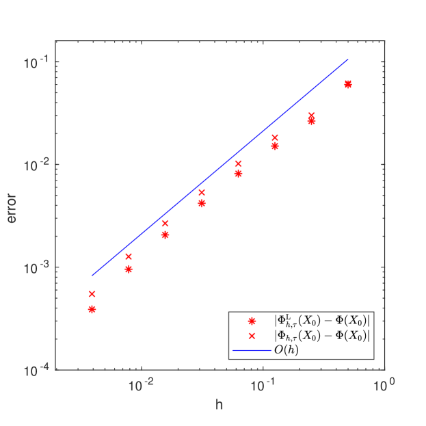
Figure 1. Estimates of the errors $|\Phi^{\mathrm{L}}(X_{0})-\Phi^{T}(X_{0})|$ and $|\Phi_{h,\tau}(X_{0})-\Phi(X_{0})|$ for a fixed $X_{0}\in H$.

Here we have replaced $\Phi(X_{0})$ with the reference solution $\Phi_{h,\tau}(X_{0})$ computed with $h=2^{-10}$ and $\tau=h^{2}$. All matrices and vectors are computed exactly, which is possible by our choice of $U$, except for the initial value, which is interpolated onto the finite element space. Since $b<\infty$ for all $\beta<1/2$, we expect from Corollary 4.3 and Corollary 5.3 a convergence rate of essentially $\mathcal{O}(h)$. The results of Figure 1 are consistent with this expectation.

6.2. Comparison to the Monte Carlo method

The most straightforward way of utilizing a finite element method for the approximation of $\Phi(x)$ in (4), with $x$ fixed, is by a Monte Carlo method, i.e., by computing

(43) $$\Phi_{h,\tau,M}^{\mathrm{MC}}(x)=M^{-1}\sum_{j=1}^{M}\left(\left\|GX_{h,\tau}^{N_{\tau},x,(j)}\right\|^{2}+\sum_{n=0}^{N_{\tau}-1}\tau\left\|RX_{h,\tau}^{n,x,(j)}\right\|^{2}\right).$$

Here $M$ is the number of iid samples $(X_{h,\tau}^{n,x,(j)})_{j=1}^{M}$ of $X_{h,\tau}^{n,x}$ computed by the recursion (37). The Monte Carlo method has a low memory requirement, is easy to parallelize and can be improved by multilevel methods (see, e.g., [22] as well as the comment at the end of the next section). There are, however, certain situations in which the Lyapunov method of computing $\Phi^{\mathrm{L}}_{h,\tau}(x)$ is preferable for the approximation of $\Phi(x)$, which we now outline.

6.2.1. Empirical stability analysis

The zero solution $X(t)=0$ to an SPDE with multiplicative noise such as (1) (or a discretization thereof) can be simultaneously asymptotically stable in a ${\mathbf{P}}$-a.s. sense and unstable in a mean square sense. In a Monte Carlo type method, this results in the number of samples needed for a satisfactory approximation in practice being prohibitively large. We discuss this challenge to such methods in detail, in the setting that $R=0$ and $G=\mathrm{id}_{H}$.

Consider the rescaled semidiscrete stochastic heat equation

(44) $$\mathrm{d}X_{h}(t)+\lambda A_{h}X_{h}(t)\,\mathrm{d}t=\sigma P_{h}B(X_{h}(t))\,\mathrm{d}W(t).$$

Here, $\lambda,\sigma\geq 0$ while all other parameters are as in Section 6.1.2. Following [1], the zero solution to (44) is said to be asymptotically stable ${\mathbf{P}}$-a.s. if, for any $\epsilon\in(0,1)$ and $\epsilon^{\prime}>0$, there exist

1. $\delta>0$ such that if $\|X_{h}(0)\|<\delta$, then ${\mathbf{P}}(\|X_{h}(t)\|>\epsilon^{\prime})<\epsilon$ for all $t\geq 0$ and

2. $\delta^{\prime}>0$ such that for any initial value $X_{h}(0)$ satisfying $\|X_{h}(0)\|<\delta^{\prime}$ ${\mathbf{P}}$-a.s., $\lim_{t\to\infty}\|X_{h}(t)\|=0$ ${\mathbf{P}}$-a.s.

It is said to be asymptotically mean square stable if for every $\epsilon>0$, there exist

1. $\delta>0$ such that if $\|X_{h}(0)\|<\delta$ then ${\mathbb{E}}[\|X_{h}(t)\|^{2}]<\epsilon$ for all $t\geq 0$ and

2. $\delta^{\prime}>0$ such that if $\|X_{h}(0)\|<\delta^{\prime}$ then $\lim_{t\to\infty}{\mathbb{E}}[\|X_{h}(t)\|^{2}]=0$.

In [1], the authors consider a discretized stochastic heat equation, similar to (44) but with finite differences instead of finite elements. They prove that as $\sigma$ increases, the zero solution becomes simultaneously asymptotically stable ${\mathbf{P}}$-a.s. and asymptotically mean square unstable. While their results do not directly translate to our setting, we also expect that for large $T$ and $\sigma$, ${\mathbb{E}}[\|X_{h}(T)\|^{2}]$ becomes very big while most sample paths of $X_{h}$ are very small, possibly zero within machine accuracy. If the time discretization of $X_{h}$ shares this property as assumed in [1], $\Phi_{h,\tau,M}^{\mathrm{MC}}(X_{0})$ approximates ${\mathbb{E}}[\|X_{h}(T)\|^{2}]$, and therefore also ${\mathbb{E}}[\|X(T)\|^{2}]$, poorly.

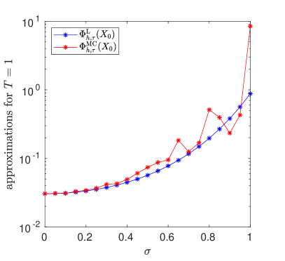
(a) $T=1$

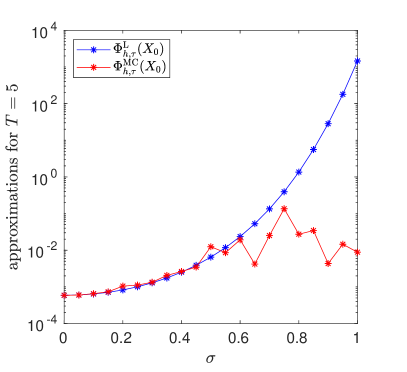
(b) $T=5$

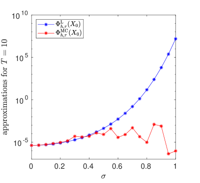
(c) $T=10$

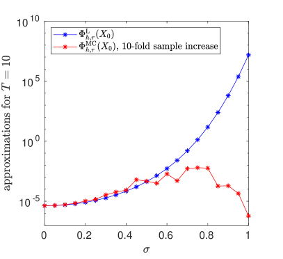
(d) $T=10$, 10-fold increase of sample size

Figure 2. Lyapunov and Monte Carlo approximations of $\mathbb{E}[\|X(T)\|^{2}]$ for $T=1,5$ and $10$ and $\sigma\in[0,1]$.

To investigate this in practice, we choose $X_{0}$ and $\lambda=0.05$ as in Section 6.1.2 and compute approximations of ${\mathbb{E}}[\|X(T)\|^{2}]$ for various values of $\sigma$ and $T$. The results from the Lyapunov method and the Monte Carlo method are compared. We choose $h=2^{-5}$ and $\tau=h^{2}$ for both methods, with $M=h^{-2}=1024$ samples in the Monte Carlo method. In Figure 2(a) we see the results of the two methods for $T=1$ and $\sigma\in[0,1]$. They seem to agree reasonably well for small values of $\sigma$, while the variance of $\Phi_{h,\tau,M}^{\mathrm{MC}}(X_{0})$ increases as $\sigma$ increases. For moderately larger values of $T$, we already see the consequences of the mean square instability and the ${\mathbf{P}}$-a.s. stability of the zero solution to (44). In Figure 2(b), with $T=5$, the difference between the two approximations is of several orders of magnitude. This behavior is even more pronounced for $T=10$ in Figure 2(c). Even if we increase the number of samples to $M=10h^{-2}$ (see Figure 2(d)), the results do not improve for $\sigma\approx 1$. In other words, even for moderately large values of $\sigma$ and $T$, the Monte Carlo method fails to give reliable results. As noted in [1], replacing this simple Monte Carlo estimator with a multilevel Monte Carlo method does not solve this issue. Indeed, if empirical variances are used to estimate the number of samples needed at each level this method can suffer even more from this stability problem.

6.2.2. Computational complexity comparison

Even under parameter choices for which the stability problems outlined in the previous section do not occur, there may be other reasons for why one would prefer to approximate ${\mathbb{E}}[\|X(T)\|^{2}]$ by means of the Lyapunov method rather than by Monte Carlo. First, the computation of $\Phi_{h,\tau,M}^{\mathrm{MC}}(x)$ can be expensive if $R$ is a non-local operator. Then the matrix ${\mathbf{R}}_{h}$ is typically dense. This matrix is applied for the computation of the term containing $R$ in (43) a total of $M\times N_{\tau}$ times. By the law of large numbers, $M$ should be chosen to be proportional to the inverse of the square root of the weak error in Corollary 5.3 in order for the Monte Carlo error not to asymptotically dominate the full mean squared error. Therefore, the computational cost can become prohibitively large.

Second, the Lyapunov method yields a way of approximating $\Phi(x)$ for all $x\in H$ simultaneously. The Monte Carlo method can be adapted to this setting by iterating (37) to obtain

$$X_{h,\tau}^{n,x}=\left(\prod_{j=0}^{n-1}S_{h,\tau}\left(P_{h}+BP_{h}(\cdot)\Delta W^{j}\right)\right)P_{h}x=:F^{n}_{h,\tau}P_{h}x$$

and then computing

$$\Phi_{h,\tau,M}^{\mathrm{MC}}(\cdot)$$

$$\qquad=\left\langle M^{-1}\sum_{j=1}^{M}\left((F^{N_{\tau},(j)}_{h,\tau})^{*}G^{*}GF^{N_{\tau},(j)}_{h,\tau}+\sum_{n=0}^{N_{\tau}-1}\tau(F^{n,(j)}_{h,\tau})^{*}R^{*}RF^{n,(j)}_{h,\tau}\right)P_{h}\cdot,\cdot\right\rangle.$$

However, forming the matrix corresponding to the sum of operators requires, again, the multiplication and addition of dense matrices, leading to great costs in terms of both computational power and memory. In fact, in the setting of the simulations of Section 6.1.2, it can be seen that the computational cost of $\Phi^{\mathrm{L}}_{h,\tau}$ is $\mathcal{O}(h^{-4})$. This can be compared to $\mathcal{O}(h^{-6})$ for $\Phi_{h,\tau,M}^{\mathrm{MC}}(\cdot)$, the cost of the iterated Monte Carlo method if one chooses $M\simeq h^{-2}$ so that the additional Monte Carlo error does not dominate.

In conclusion, we have demonstrated that there may be several situations in which the Lyapunov method of computing $\Phi^{\mathrm{L}}_{h,\tau}(X_{0})$ is preferable for the approximation of $\Phi(X_{0})$ compared to a Monte Carlo method. It should, however, be noted that it may be fruitful to combine these methods. For example, the Lyapunov method, computed at a coarse grid, may be used to indicate the presence of mean square instability combined with ${\mathbf{P}}$-a.s. stability in a system such as (44), suggesting that remedies such as the ones discussed in [1] should be taken.

Appendix A Proofs for Section 3.1

A.1. Proof of Theorem 3.1

As a first step we prove a result that is needed to ensure that the integrals in the proof of Theorem 3.1 are well-defined. The setting and notation is the same as in Sections 2 and 3 of the main text.

Lemma A.1.

For all $t\in\mathbb{T}_{0}$, $\theta_{1},\theta_{2}\geq 0$ and $\Upsilon\in{\mathcal{V}}$ the mappings

$$[0,t)\ni s\mapsto A^{\frac{\theta_{1}}{2}}S(t-s)R^{*}RS(t-s)A^{\frac{\theta_{2}}{2}}\in{\mathcal{L}}(H)$$

and

$$(0,t)\ni s\mapsto A^{\frac{\theta_{1}}{2}}S(t-s)B^{*}\Upsilon(s)BS(t-s)A^{\frac{\theta_{2}}{2}}\in{\mathcal{L}}(H)$$

are strongly continuous.

Proof.

We prove the strong continuity of the second mapping in detail. The proof of the first is done in the same way.

The second mapping is a composition of the mappings $(0,t)\ni s\mapsto A^{\theta_{1}/2}S(t-s)\in{\mathcal{L}}(H)$, $(0,t)\ni s\mapsto B^{*}\Upsilon(s)B\in{\mathcal{L}}(H)$ and $(0,t)\ni s\mapsto S(t-s)A^{\theta_{2}/2}\in{\mathcal{L}}(H)$. The first and third are strongly continuous as mappings $(0,t)\to{\mathcal{L}}(\dot{H}^{\theta_{1}},H)$ and $(0,t)\to{\mathcal{L}}(\dot{H}^{\theta_{2}},H)$, respectively. This property can be extended to $(0,t)\to{\mathcal{L}}(H)$ in both cases by considering an approximating sequence in $\dot{H}^{\theta_{1}}$ and $\dot{H}^{\theta_{2}}$, respectively. Using (7), the strong continuity of $S$ and uniform continuity of $\Upsilon$ we obtain for $s,\tilde{s}\in(0,t)$ and $\phi\in H$ that

$$\big{\|}\big{(}A^{\frac{\theta_{1}}{2}}S(t-s)B^{*}\Upsilon(s)BS(t-s)A^{\frac{\theta_{2}}{2}}-A^{\frac{\theta_{1}}{2}}S(t-\tilde{s})B^{*}\Upsilon(\tilde{s})BS(t-\tilde{s})A^{\frac{\theta_{2}}{2}}\big{)}\phi\big{\|}$$

$$\qquad\leq\big{\|}\big{(}A^{\frac{\theta_{1}}{2}}S(t-s)-A^{\theta_{1}}S(t-\tilde{s})\big{)}B^{*}\Upsilon(s)BS(t-s)A^{\frac{\theta_{2}}{2}}\phi\big{\|}$$

$$\qquad\quad+\big{\|}A^{\frac{\theta_{1}}{2}}S(t-\tilde{s})B^{*}(\Upsilon(s)-\Upsilon(\tilde{s}))BS(t-s)A^{\frac{\theta_{2}}{2}}\phi\big{\|}$$

$$\qquad\quad+\big{\|}A^{\frac{\theta_{1}}{2}}S(t-\tilde{s})B^{*}\Upsilon(\tilde{s})B\big{(}S(t-s)A^{\frac{\theta_{2}}{2}}-S(t-\tilde{s})A^{\frac{\theta_{2}}{2}}\big{)}\phi\big{\|}$$

$$\qquad\leq\big{\|}\big{(}A^{\frac{\theta_{1}}{2}}S(t-s)-A^{\frac{\theta_{1}}{2}}S(t-\tilde{s})\big{)}B^{*}\Upsilon(s)BS(t-s)A^{\frac{\theta_{2}}{2}}\phi\big{\|}$$

$$\qquad\quad+b^{2}C_{\theta_{1}}C_{\theta_{2}}(t-\tilde{s})^{-\frac{\theta_{1}}{2}}(t-s)^{-\frac{\theta_{2}}{2}}\big{\|}A^{\frac{1-\beta}{2}}(\Upsilon(s)-\Upsilon(\tilde{s}))A^{\frac{1-\beta}{2}}\big{\|}_{{\mathcal{L}}(H)}\|\phi\|$$

$$\qquad\quad+b^{2}C_{\theta_{1}}(t-\tilde{s})^{-\frac{\theta_{1}}{2}}\tilde{s}^{\beta-1}{|\kern-1.07639pt|\kern-1.07639pt|}\Upsilon{|\kern-1.07639pt|\kern-1.07639pt|}_{0}\big{\|}\big{(}S(t-s)A^{\frac{\theta_{2}}{2}}-S(t-\tilde{s})A^{\frac{\theta_{2}}{2}}\big{)}\phi\big{\|}$$

with the constant notation introduced in Section 2. Since $B^{*}\Upsilon(s)BS(t-s)A^{\theta_{2}/2}\phi\in H$ and $S$ is strongly continuous and since $\Upsilon\colon\mathbb{T}_{0}\to{\mathcal{L}}(\dot{H}^{\beta-1},\dot{H}^{1-\beta})$ is uniformly continuous, the right hand side converges to zero as $\tilde{s}$ tends to $s$. This completes the proof. ∎

The rest of the proof of Theorem 3.1 is based on a global fixed point argument in ${\mathcal{V}}$. Equation (19) is written in the form of a fixed point equation

$$L=\mathcal{H}(L)=\mathcal{I}+\mathcal{J}+\mathcal{K}(L),$$

with $\mathcal{I},\mathcal{J}\in{\mathcal{V}}$, $\mathcal{K}\colon{\mathcal{V}}\to{\mathcal{V}}$ acting on $\phi\in H$ by

$$\mathcal{I}(t)\phi =S(t)G^{*}GS(t)\phi,$$

$$\mathcal{J}(t)\phi =\int_{0}^{t}S(t-s)R^{*}RS(t-s)\phi\,\mathrm{d}s,$$

$$\mathcal{K}(\Upsilon)(t)\phi =\int_{0}^{t}S(t-s)B^{*}\Upsilon(s)BS(t-s)\phi\,\mathrm{d}s.$$

Existence of a unique solution in ${\mathcal{V}}$ follows by the Banach fixed point theorem by proving that $\mathcal{H}$ is well-defined and that for some $\sigma>0$ the fixed point map $\mathcal{H}$ is a contraction, i.e., that there exists $\eta\in(0,1)$ such that for all $\Upsilon_{1},\Upsilon_{2}\in{\mathcal{V}}$

(45) $${|\kern-1.07639pt|\kern-1.07639pt|}\mathcal{H}(\Upsilon_{1})-\mathcal{H}(\Upsilon_{2}){|\kern-1.07639pt|\kern-1.07639pt|}_{\sigma}={|\kern-1.07639pt|\kern-1.07639pt|}\mathcal{K}(\Upsilon_{1})-\mathcal{K}(\Upsilon_{2}){|\kern-1.07639pt|\kern-1.07639pt|}_{\sigma}={|\kern-1.07639pt|\kern-1.07639pt|}\mathcal{K}(\Upsilon_{1}-\Upsilon_{2}){|\kern-1.07639pt|\kern-1.07639pt|}_{\sigma}\leq\eta\,{|\kern-1.07639pt|\kern-1.07639pt|}\Upsilon_{1}-\Upsilon_{2}{|\kern-1.07639pt|\kern-1.07639pt|}_{\sigma}.$$

The proof is organized as follows: We start by proving that ${|\kern-1.07639pt|\kern-1.07639pt|}\mathcal{I}{|\kern-1.07639pt|\kern-1.07639pt|}_{0}+{|\kern-1.07639pt|\kern-1.07639pt|}\mathcal{J}{|\kern-1.07639pt|\kern-1.07639pt|}_{0}+{|\kern-1.07639pt|\kern-1.07639pt|}\mathcal{K}{|\kern-1.07639pt|\kern-1.07639pt|}_{0}<\infty$ and continue by showing that $\mathcal{I}$, $\mathcal{J}$ and $\mathcal{K}(\Upsilon)$ with $\Upsilon\in{\mathcal{V}}$ are strongly and uniformly continuous on $\mathbb{T}$ and $\mathbb{T}_{0}$, respectively. From this we conclude that $\mathcal{I}$, $\mathcal{J}$, $\mathcal{K}$ are well-defined and derive bounds to show the contraction property (45) of $\mathcal{H}$ and the claimed regularity estimates.

To prove that ${|\kern-1.07639pt|\kern-1.07639pt|}\mathcal{I}{|\kern-1.07639pt|\kern-1.07639pt|}_{0}<\infty$ we observe, using (7), that for all $\theta_{1},\theta_{2}\geq 0$ and $t\in\mathbb{T}_{0}$

(46) $$\big{\|}A^{\frac{\theta_{1}}{2}}\mathcal{I}(t)A^{\frac{\theta_{2}}{2}}\big{\|}_{{\mathcal{L}}(H)}\leq g^{2}\big{\|}A^{\frac{\theta_{1}}{2}}S(t)\big{\|}_{{\mathcal{L}}(H)}\big{\|}S(t)A^{\frac{\theta_{2}}{2}}\big{\|}_{{\mathcal{L}}(H)}\leq g^{2}C_{\theta_{1}}C_{\theta_{2}}t^{-\frac{\theta_{1}+\theta_{2}}{2}}.$$

Setting $\theta_{1}=\theta_{2}=1-\beta$ and $\theta_{1}=\theta_{2}=0$, respectively, shows the desired bound

(47) $${|\kern-1.07639pt|\kern-1.07639pt|}\mathcal{I}{|\kern-1.07639pt|\kern-1.07639pt|}_{0}\leq g^{2}(C_{0}^{2}+C_{1-\beta}^{2})<\infty.$$

For $\mathcal{J}$ we use (7) to obtain that for all $\theta_{1},\theta_{2}\geq 0$, $t\in\mathbb{T}_{0}$, $s\in[0,t)$ and $\phi\in H$

(48) $$\big{\|}A^{\frac{\theta_{1}}{2}}S(t-s)R^{*}RS(t-s)A^{\frac{\theta_{2}}{2}}\phi\big{\|}\leq r^{2}C_{\theta_{1}}C_{\theta_{2}}\|\phi\|(t-s)^{-\frac{\theta_{1}+\theta_{2}}{2}}.$$

Together with the strong continuity of the mapping shown in Lemma A.1, this bound implies that $A^{\theta_{1}/2}S(t-\cdot)R^{*}RS(t-\cdot)A^{\theta_{2}/2}\phi\in L^{1}([0,t],H)$ when $\theta_{1},\theta_{2}\in[0,2)$ with $\theta_{1}+\theta_{2}<2$, and in particular that the Bochner integral in $\mathcal{J}$ is well-defined. It also shows that $\mathcal{J}$ can be extended to a mapping $\mathbb{T}_{0}\to{\mathcal{L}}(\dot{H}^{-\theta_{2}},\dot{H}^{\theta_{1}})$. Next, for $t\in\mathbb{T}_{0}$

(49) $$\begin{split}\big{\|}A^{\frac{\theta_{1}}{2}}\mathcal{J}(t)A^{\frac{\theta_{2}}{2}}\big{\|}_{{\mathcal{L}}(H)}&=\sup_{\phi\in H,\|\phi\|=1}\Big{\|}\int_{0}^{t}A^{\frac{\theta_{1}}{2}}S(t-s)R^{*}RS(t-s)A^{\frac{\theta_{2}}{2}}\phi\,\mathrm{d}s\Big{\|}\\ &\leq\int_{0}^{t}\sup_{\phi\in H,\|\phi\|=1}\Big{\|}A^{\frac{\theta_{1}}{2}}S(t-s)R^{*}RS(t-s)A^{\frac{\theta_{2}}{2}}\phi\Big{\|}\,\mathrm{d}s\\ &=\int_{0}^{t}\Big{\|}A^{\frac{\theta_{1}}{2}}S(t-s)R^{*}RS(t-s)A^{\frac{\theta_{2}}{2}}\Big{\|}_{{\mathcal{L}}(H)}\,\mathrm{d}s.\end{split}$$

Using (48) we have for $t\in\mathbb{T}_{0}$

(50) $$\big{\|}A^{\frac{\theta_{1}}{2}}\mathcal{J}(t)A^{\frac{\theta_{2}}{2}}\big{\|}_{{\mathcal{L}}(H)}\leq\frac{2r^{2}C_{\theta_{1}}C_{\theta_{2}}}{2-\theta_{1}-\theta_{2}}\,t^{1-\frac{\theta_{1}-\theta_{2}}{2}}.$$

Setting $\theta_{1}=\theta_{2}=1-\beta$ and $\theta_{1}=\theta_{2}=0$, respectively, shows that

(51) $${|\kern-1.07639pt|\kern-1.07639pt|}\mathcal{J}{|\kern-1.07639pt|\kern-1.07639pt|}_{0}\leq r^{2}\left(C_{0}^{2}T+C_{1-\beta}^{2}\beta^{-1}T^{\beta}\right)<\infty.$$

We now turn our attention to $\mathcal{K}$. For all $\theta_{1},\theta_{2}\geq 0$, $t\in\mathbb{T}_{0}$, $s\in(0,t)$, $\Upsilon\in{\mathcal{V}}$, and $\phi\in H$, we have by using (7) that

(52) $$\begin{split}&\big{\|}A^{\frac{\theta_{1}}{2}}S(t-s)B^{*}\Upsilon(s)BS(t-s)A^{\frac{\theta_{2}}{2}}\phi\big{\|}\\ &\qquad\leq b^{2}C_{\theta_{1}}C_{\theta_{2}}{|\kern-1.07639pt|\kern-1.07639pt|}\Upsilon{|\kern-1.07639pt|\kern-1.07639pt|}_{\sigma}\|\phi\|e^{\sigma s}s^{\beta-1}(t-s)^{-\frac{\theta_{1}+\theta_{2}}{2}}.\end{split}$$

Combining this with Lemma A.1 implies that for $\theta_{1},\theta_{2}\in[0,2)$ with $\theta_{1}+\theta_{2}<2$, $A^{\theta_{1}/2}S(t-\cdot)B^{*}\Upsilon(\cdot)BS(t-\cdot)A^{\theta_{2}/2}\phi\in L^{1}([0,t],H)$ and in particular that the Bochner integral in $\mathcal{K}$ is well-defined. Similarly to $\mathcal{J}$, it also implies that $\mathcal{K}(\Upsilon)$ can be extended to $\mathbb{T}\to{\mathcal{L}}(\dot{H}^{-\theta_{2}},\dot{H}^{\theta_{1}})$. Using (52) we obtain, similarly to (49), the bound

(53) $$\big{\|}A^{\frac{\theta_{1}}{2}}\mathcal{K}(\Upsilon)(t)A^{\frac{\theta_{2}}{2}}\big{\|}_{{\mathcal{L}}(H)}\leq b^{2}C_{\theta_{1}}C_{\theta_{2}}\Bigg{(}\int_{0}^{t}e^{\sigma s}s^{\beta-1}(t-s)^{-\frac{\theta_{1}+\theta_{2}}{2}}\,\mathrm{d}s\Bigg{)}{|\kern-1.07639pt|\kern-1.07639pt|}\Upsilon{|\kern-1.07639pt|\kern-1.07639pt|}_{\sigma}.$$

For the case $\sigma=0$, we conclude from (5) that

(54) $$\big{\|}A^{\frac{\theta_{1}}{2}}\mathcal{K}(\Upsilon)(t)A^{\frac{\theta_{2}}{2}}\big{\|}_{{\mathcal{L}}(H)}\leq b^{2}C_{\theta_{1}}C_{\theta_{2}}t^{\beta-\frac{\theta_{1}+\theta_{2}}{2}}{\mathbf{B}}\Big{(}\beta,1-\frac{\theta_{1}+\theta_{2}}{2}\Big{)}{|\kern-1.07639pt|\kern-1.07639pt|}\Upsilon{|\kern-1.07639pt|\kern-1.07639pt|}_{0}.$$

Setting again $\theta_{1}=\theta_{2}=1-\beta$ and $\theta_{1}=\theta_{2}=0$, respectively, yields

(55) $${|\kern-1.07639pt|\kern-1.07639pt|}\mathcal{K}(\Upsilon){|\kern-1.07639pt|\kern-1.07639pt|}_{0}\leq b^{2}\Big{(}C_{0}^{2}{\mathbf{B}}(\beta,1)T+C_{1-\beta}^{2}{\mathbf{B}}(\beta,\beta)T^{\beta}\Big{)}{|\kern-1.07639pt|\kern-1.07639pt|}\Upsilon{|\kern-1.07639pt|\kern-1.07639pt|}_{0}<\infty$$

and combining (47), (51), (55) implies that ${|\kern-1.07639pt|\kern-1.07639pt|}\mathcal{H}(\Upsilon){|\kern-1.07639pt|\kern-1.07639pt|}_{0}<\infty$.

Next we show continuity of $\mathcal{I}$, $\mathcal{J}$ and $\mathcal{K}(\Upsilon)$ on $\mathbb{T}_{0}$ and $\mathbb{T}$. For this purpose we prove Hölder continuity in operator norms on $(0,T)$ and strong continuity at zero separately. The Hölder continuity also implies (ii) once existence and uniqueness have been established. For all $\theta_{1},\theta_{2}\geq 0$, $\xi\in[0,1]$ and $t_{1},t_{2}\in\mathbb{T}_{0}$ with $t_{1}<t_{2}$, we bound using (7), (8) and the semigroup property of $S$

(56) $$\begin{split}&\big{\|}A^{\frac{\theta_{1}}{2}}\big{(}\mathcal{I}(t_{2})-\mathcal{I}(t_{1})\big{)}A^{\frac{\theta_{2}}{2}}\big{\|}_{{\mathcal{L}}(H)}\\ &\quad\leq g^{2}\big{\|}A^{\frac{\theta_{1}}{2}}S(t_{1})A^{\xi}\big{\|}_{{\mathcal{L}}(H)}\big{\|}A^{-\xi}\big{(}S(t_{2}-t_{1})-\mathrm{id}_{H}\big{)}\big{\|}_{{\mathcal{L}}(H)}\big{\|}S(t_{2})A^{\frac{\theta_{2}}{2}}\big{\|}_{{\mathcal{L}}(H)}\\ &\qquad+g^{2}\big{\|}A^{\frac{\theta_{1}}{2}}S(t_{1})\big{\|}_{{\mathcal{L}}(H)}\big{\|}\big{(}S(t_{2}-t_{1})-\mathrm{id}_{H}\big{)}A^{-\xi}\big{\|}_{{\mathcal{L}}(H)}\big{\|}A^{\xi}S(t_{1})A^{\frac{\theta_{2}}{2}}\big{\|}_{{\mathcal{L}}(H)}\\ &\quad\leq g^{2}C_{2\xi}\big{(}C_{\theta_{1}+2\xi}C_{\theta_{2}}+C_{\theta_{1}}C_{\theta_{2}+2\xi}\big{)}t_{1}^{-\frac{\theta_{1}+\theta_{2}}{2}-\xi}|t_{2}-t_{1}|^{\xi}.\end{split}$$

This shows in particular strong continuity $\mathcal{I}\in\mathcal{C}_{\mathrm{s}}(\mathbb{T}_{0},{\mathcal{L}}(H))$ and uniform continuity $\mathcal{I}\in\mathcal{C}(\mathbb{T}_{0},{\mathcal{L}}(\dot{H}^{\beta-1},\dot{H}^{1-\beta}))$. To prove $\mathcal{I}\in{\mathcal{V}}$ it remains to prove strong continuity $\mathcal{I}\in\mathcal{C}_{\mathrm{s}}(\mathbb{T},{\mathcal{L}}(H))$ and for this we have by the strong continuity (8) of $S$ for $\phi\in H$

$$\lim_{t\to 0}\big{\|}(\mathcal{I}(t)-\mathcal{I}(0))\phi\big{\|} \leq\lim_{t\to 0}\big{\|}(S(t)-\mathrm{id}_{H})G^{*}GS(t)\phi\big{\|}$$

$$\quad+\lim_{t\to 0}\big{\|}G^{*}G(S(t)-\mathrm{id}_{H})\phi\big{\|}=0.$$

Let us continue with $\mathcal{K}$. We observe that for $\phi\in H$, $\Upsilon\in{\mathcal{V}}$ and $t_{1},t_{2}\in\mathbb{T}_{0}$ with $t_{1}<t_{2}$ that

$$\big{(}\mathcal{K}(\Upsilon)(t_{2})-\mathcal{K}(\Upsilon)(t_{1})\big{)}\phi$$

$$\qquad=\int_{0}^{t_{1}}(S(t_{2}-s)-S(t_{1}-s))B^{*}\Upsilon(s)BS(t_{2}-s)\phi\,\mathrm{d}s$$

$$\qquad\quad+\int_{0}^{t_{1}}S(t_{1}-s)B^{*}\Upsilon(s)B(S(t_{2}-s)-S(t_{1}-s))\phi\,\mathrm{d}s$$

$$\qquad\quad+\int_{t_{1}}^{t_{2}}S(t_{2}-s)B^{*}\Upsilon(s)BS(t_{2}-s)\phi\,\mathrm{d}s.$$

Similarly to (49), this yields by using the semigroup property of $S$ and (8) that

$$\big{\|}A^{\frac{\theta_{1}}{2}}\big{(}\mathcal{K}(\Upsilon)(t_{2})-\mathcal{K}(\Upsilon)(t_{1})\big{)}A^{\frac{\theta_{2}}{2}}\big{\|}_{{\mathcal{L}}(H)}$$

$$\qquad\leq b^{2}\int_{0}^{t_{1}}\big{\|}A^{\frac{\theta_{1}}{2}}S(t_{1}-s)A^{\xi}\big{\|}_{{\mathcal{L}}(H)}\big{\|}A^{-\xi}\big{(}S(t_{2}-t_{1})-\mathrm{id}_{H}\big{)}\big{\|}_{{\mathcal{L}}(H)}$$

$$\qquad\qquad\qquad\quad\times\big{\|}A^{\frac{1-\beta}{2}}\Upsilon(s)A^{\frac{1-\beta}{2}}\big{\|}_{{\mathcal{L}}(H)}\big{\|}S(t_{2}-s)A^{\frac{\theta_{2}}{2}}\big{\|}_{{\mathcal{L}}(H)}\,\mathrm{d}s$$

$$\qquad\quad+b^{2}\int_{0}^{t_{1}}\big{\|}A^{\frac{\theta_{1}}{2}}S(t_{1}-s)\big{\|}_{{\mathcal{L}}(H)}\big{\|}A^{\frac{1-\beta}{2}}\Upsilon(s)A^{\frac{1-\beta}{2}}\big{\|}_{{\mathcal{L}}(H)}$$

$$\qquad\qquad\qquad\quad\times\big{\|}S(t_{1}-s)A^{\xi+\frac{\theta_{2}}{2}}\big{\|}_{{\mathcal{L}}(H)}\big{\|}A^{-\xi}\big{(}S(t_{2}-t_{1})-\mathrm{id}_{H}\big{)}\big{\|}_{{\mathcal{L}}(H)}\,\mathrm{d}s$$

$$\qquad\quad+b^{2}\int_{t_{1}}^{t_{2}}\big{\|}A^{\frac{\theta_{1}}{2}}S(t_{2}-s)\big{\|}_{{\mathcal{L}}(H)}\big{\|}A^{\frac{1-\beta}{2}}\Upsilon(s)A^{\frac{1-\beta}{2}}\big{\|}_{{\mathcal{L}}(H)}$$

$$\qquad\qquad\qquad\quad\times\big{\|}S(t_{2}-s)A^{\frac{\theta_{2}}{2}}\big{\|}_{{\mathcal{L}}(H)}\,\mathrm{d}s$$

and thus using (7) and (8)

$$\big{\|}A^{\frac{\theta_{1}}{2}}\big{(}\mathcal{K}(\Upsilon)(t_{2})-\mathcal{K}(\Upsilon)(t_{1})\big{)}A^{\frac{\theta_{2}}{2}}\big{\|}_{{\mathcal{L}}(H)}$$

$$\qquad\leq b^{2}C_{\xi}C_{\theta_{1}+2\xi}C_{\theta_{2}}{|\kern-1.07639pt|\kern-1.07639pt|}\Upsilon{|\kern-1.07639pt|\kern-1.07639pt|}_{0}\Bigg{(}\int_{0}^{t_{1}}s^{\beta-1}(t_{1}-s)^{-\frac{\theta_{1}}{2}-\xi}(t_{2}-s)^{-\frac{\theta_{2}}{2}}\,\mathrm{d}s\Bigg{)}|t_{2}-t_{1}|^{\xi}$$

$$\qquad\quad+b^{2}C_{2\xi}C_{\theta_{1}}C_{\theta_{2}+2\xi}{|\kern-1.07639pt|\kern-1.07639pt|}\Upsilon{|\kern-1.07639pt|\kern-1.07639pt|}_{0}\Bigg{(}\int_{0}^{t_{1}}s^{\beta-1}(t_{1}-s)^{-\frac{\theta_{1}+\theta_{2}}{2}-\xi}\,\mathrm{d}s\Bigg{)}|t_{2}-t_{1}|^{\xi}$$

$$\qquad\quad+b^{2}C_{\theta_{1}}C_{\theta_{2}}{|\kern-1.07639pt|\kern-1.07639pt|}\Upsilon{|\kern-1.07639pt|\kern-1.07639pt|}_{0}\int_{t_{1}}^{t_{2}}s^{\beta-1}(t_{2}-s)^{-\frac{\theta_{1}+\theta_{2}}{2}}\,\mathrm{d}s.$$

Since for $s\in[0,t_{1})$, $(t_{2}-s)^{-\theta_{2}/2}\leq(t_{1}-s)^{-\theta_{2}/2}$ and for $s\in(t_{1},t_{2}]$, $s^{\beta-1}\leq T^{\beta}t_{1}^{-\xi-(\theta_{1}+\theta_{2})/2}s^{\xi+(\theta_{1}+\theta_{2})/2-1}\leq T^{\beta}t_{1}^{-\xi-(\theta_{1}+\theta_{2})/2}(s-t_{1})^{\xi+(\theta_{1}+\theta_{2})/2-1}$, we have

$$\big{\|}A^{\frac{\theta_{1}}{2}}\big{(}\mathcal{K}(\Upsilon)(t_{2})-\mathcal{K}(\Upsilon)(t_{1})\big{)}A^{\frac{\theta_{2}}{2}}\big{\|}_{{\mathcal{L}}(H)}$$

$$\,\leq b^{2}C_{2\xi}\big{(}C_{\theta_{1}+2\xi}C_{\theta_{2}}+C_{\theta_{1}}C_{\theta_{2}+2\xi}\big{)}{|\kern-1.07639pt|\kern-1.07639pt|}\Upsilon{|\kern-1.07639pt|\kern-1.07639pt|}_{0}\Bigg{(}\int_{0}^{t_{1}}s^{\beta-1}(t_{1}-s)^{-\frac{\theta_{1}+\theta_{2}}{2}-\xi}\,\mathrm{d}s\Bigg{)}|t_{2}-t_{1}|^{\xi}$$

$$\,\quad+b^{2}C_{\theta_{1}}C_{\theta_{2}}{|\kern-1.07639pt|\kern-1.07639pt|}\Upsilon{|\kern-1.07639pt|\kern-1.07639pt|}_{0}T^{\beta}t_{1}^{-\xi-\frac{\theta_{1}+\theta_{2}}{2}}\int_{t_{1}}^{t_{2}}(s-t_{1})^{\xi+\frac{\theta_{1}+\theta_{2}}{2}-1}(t_{2}-s)^{-\frac{\theta_{1}+\theta_{2}}{2}}\,\mathrm{d}s.$$

Using (5) we therefore obtain

(57) $$\big{\|}A^{\theta_{1}}\big{(}\mathcal{K}(\Upsilon)(t_{2})-\mathcal{K}(\Upsilon)(t_{1})\big{)}A^{\theta_{2}}\big{\|}_{{\mathcal{L}}(H)}\lesssim t_{1}^{-\frac{\theta_{1}+\theta_{2}}{2}-\xi}|t_{2}-t_{1}|^{\xi}.$$

This implies the desired continuity on $\mathbb{T}_{0}$. For the continuity at zero, we use (7) to see that

$$\big{\|}(\mathcal{K}(\Upsilon)(t)-\mathcal{K}(\Upsilon)(0))\phi\big{\|}=\Big{\|}\int_{0}^{t}S(t-s)B^{*}\Upsilon(s)BS(t-s)\phi\,\mathrm{d}s\Big{\|}\leq\frac{b^{2}C_{0}^{2}t^{\beta}{|\kern-1.07639pt|\kern-1.07639pt|}\Upsilon{|\kern-1.07639pt|\kern-1.07639pt|}_{0}}{\beta}$$

and as a consequence $\lim_{t\to 0}\|(\mathcal{K}(\Upsilon)(t)-\mathcal{K}(\Upsilon)(0))\phi\|=0$. We conclude that $\mathcal{K}(\Upsilon)\in{\mathcal{V}}$. The proof of $\mathcal{J}\in{\mathcal{V}}$ is similar and therefore omitted. In conclusion we have shown that the fixed point map $\mathcal{H}$ is well-defined.

It remains to prove the contraction property (45). For $\sigma\in{\mathbb{R}}$ the same arguments as in the proof of [4, Theorem 2.9] imply that for all $\lambda\in[0,1)$

$$\lim_{\sigma\uparrow\infty}\Bigg{(}\sup_{t\in\mathbb{T}_{0}}t^{1-\beta}\int_{0}^{t}e^{-\sigma(t-s)}s^{\beta-1}(t-s)^{-\lambda}\,\mathrm{d}s\Bigg{)}=0.$$

Combining this with (53) implies the existence of $\sigma>0$ and $\eta\in(0,1)$ such that

$${|\kern-1.07639pt|\kern-1.07639pt|}\mathcal{K}(\Upsilon){|\kern-1.07639pt|\kern-1.07639pt|}_{\sigma} \leq b^{2}\Bigg{(}C_{0}^{2}\sup_{t\in\mathbb{T}_{0}}\int_{0}^{t}e^{-\sigma(t-s)}s^{\beta-1}\,\mathrm{d}s$$

$$\qquad+C_{1-\beta}^{2}\sup_{t\in\mathbb{T}_{0}}t^{1-\beta}\int_{0}^{t}e^{-\sigma(t-s)}s^{\beta-1}(t-s)^{\beta-1}\,\mathrm{d}s\Bigg{)}{|\kern-1.07639pt|\kern-1.07639pt|}\Upsilon{|\kern-1.07639pt|\kern-1.07639pt|}_{\sigma}\leq\eta{|\kern-1.07639pt|\kern-1.07639pt|}\Upsilon{|\kern-1.07639pt|\kern-1.07639pt|}_{\sigma}.$$

We have therefore shown that $\mathcal{H}$ is a contraction with respect to the ${|\kern-1.07639pt|\kern-1.07639pt|}\cdot{|\kern-1.07639pt|\kern-1.07639pt|}_{\sigma}$-norm for sufficiently large $\sigma>0$. The Banach fixed point theorem guarantees the existence and uniqueness of a fixed point $L$ to the mapping $\mathcal{H}$. This is the unique mild solution to (19). To prove that $L(\mathbb{T})\subset\Sigma(H)$ we consider ${\mathcal{V}}^{\prime}=\mathcal{C}_{\mathrm{s}}(\mathbb{T},\Sigma(H))\cap\mathcal{C}(\mathbb{T}_{0},{\mathcal{L}}(\dot{H}^{\beta-1},\dot{H}^{1-\beta}))\subset{\mathcal{V}}$, which is a Banach subspace of ${\mathcal{V}}$ since $\Sigma(H)$ is a closed subspace of ${\mathcal{L}}(H)$, along with the restriction $\mathcal{H}^{\prime}\colon{\mathcal{V}}^{\prime}\to{\mathcal{V}}^{\prime}$ of the fixed point map $\mathcal{H}\colon{\mathcal{V}}\to{\mathcal{V}}$ to ${\mathcal{V}}^{\prime}$. It is a contraction with the same ${|\kern-1.07639pt|\kern-1.07639pt|}\cdot{|\kern-1.07639pt|\kern-1.07639pt|}_{\sigma}$-norm as $\mathcal{H}$. One easily checks that $\mathcal{H}^{\prime}(\Upsilon^{\prime})(t)$ is self-adjoint for self-adjoint $\Upsilon^{\prime}\in{\mathcal{V}}^{\prime}$ and thus $\mathcal{H}^{\prime}$ is well-defined. Therefore, a second application of the Banach fixed point theorem yields a unique $L^{\prime}\in{\mathcal{V}}^{\prime}$ such that $\mathcal{H}^{\prime}(L^{\prime})=L^{\prime}$. Since ${\mathcal{V}}^{\prime}\subset{\mathcal{V}}$ and $L\in{\mathcal{V}}$ is unique, $L=L^{\prime}$ and thus $L(\mathbb{T})\subset\Sigma(H)$. Moreover, Theorem 3.6 in the end of this section shows that $L(\mathbb{T})\subset\Sigma^{+}(H)$ and we stress that none of the proofs of Theorem 3.2, Propositions 3.3–3.4, Lemma 3.5 leading to Theorem 3.6 relies on the positivity of $L$. The bounds (46), (50) and (54) imply (i). The bounds (56), (57) imply the Hölder regularity stated in (ii).

A.2. Proof of Theorem 3.2

We write $F=R^{*}R+B^{*}LB$ and let $L$ be a mild solution, i.e., $L$ satisfies (19). Since for all $t\in\mathbb{T}$, $\phi\in H$,

$$L(t)\phi=S(t)G^{*}GS(t)\phi+\int_{0}^{t}S(t-s)F(s)S(t-s)\phi\,\mathrm{d}s,$$

we obtain for $t+h\leq T$ and $\phi\in H$

$$L(t+h)\phi =S(h)S(t)G^{*}GS(t)S(h)\phi+\int_{0}^{t+h}S(t+h-r)F(r)S(t+h-r)\phi\,\mathrm{d}r$$

$$=S(h)L(s)S(h)\phi+\int_{t}^{t+h}S(t+h-r)F(r)S(t+h-r)\phi\,\mathrm{d}r.$$

Therefore, for $\phi,\psi\in\dot{H}^{2}$

$$\langle L(t+h)\phi,\psi\rangle =\langle L(t)S(h)\phi,S(h)\psi\rangle$$

$$\quad+\int_{t}^{t+h}\langle S(t+h-r)F(r)\phi,S(t+h-r)\psi\rangle\,\mathrm{d}r$$

and subtracting $\langle L(t)\phi,\psi\rangle$ on both sides and dividing by $h>0$ gives

$$\Bigg{\langle}\frac{L(t+h)-L(t)}{h}\phi,\psi\Bigg{\rangle} =\Bigg{\langle}L(t)\frac{S(h)-\mathrm{id}_{H}}{h}\phi,S(h)\psi\Bigg{\rangle}+\Bigg{\langle}L(t)\phi,\frac{S(h)-\mathrm{id}_{H}}{h}\psi\Bigg{\rangle}$$

$$\quad+\frac{1}{h}\int_{t}^{t+h}\langle S(t+h-r)F(r)\phi,S(t+h-r)\psi\rangle\,\mathrm{d}r.$$

The semigroup $S$ is strongly differentiable, hence weakly differentiable with derivative $\tfrac{\mathrm{d}}{\mathrm{d}t}\langle S(t)\phi,\psi\rangle=-\langle AS(t)\phi,\psi\rangle$ for $\phi,\psi\in\dot{H}^{2}$. In the limit as $h\to 0$, we obtain, by the Lebesgue differentiation theorem, the weak form (2). This completes the first direction of the proof.

Assume next that the operator-valued function $L\in{\mathcal{V}}$ satisfies for $t\in\mathbb{T}_{0}$, $\phi,\psi\in\dot{H}^{2}$ the variational equation (2). Using (6) we bound

$$\Big{|}\frac{\mathrm{d}}{\mathrm{d}t}\langle L(t)\phi,\psi\rangle\Big{|} \leq|a(L(t)\phi,\psi)|+|a(L(t)\psi,\phi)|+|\langle R\phi,R\psi\rangle|+|\langle L(t)B\phi,B\psi\rangle_{{\mathcal{L}}_{2}^{0}}|$$

$$\leq\|L(t)\|_{{\mathcal{L}}(H)}\big{(}\|A\phi\|\|\psi\|+\|\phi\|\|A\psi\|\big{)}$$

$$\quad+\big{(}r^{2}+b^{2}\big{\|}A^{\frac{1-\beta}{2}}L(t)A^{\frac{1-\beta}{2}}\big{\|}_{{\mathcal{L}}(H)}\big{)}\|\phi\|\|\psi\|$$

with $t\in\mathbb{T}_{0}$, $\phi,\psi\in\dot{H}^{2}$. Since $\|\phi\|\lesssim\|A\phi\|=\|\phi\|_{\dot{H}^{2}}$ we conclude that

$$\Big{|}\frac{\mathrm{d}}{\mathrm{d}t}\langle L(t)\phi,\psi\rangle\Big{|}\lesssim(1+t^{\beta-1})\|\phi\|_{\dot{H}^{2}}\|\psi\|_{\dot{H}^{2}}\lesssim t^{\beta-1}\|\phi\|_{\dot{H}^{2}}\|\psi\|_{\dot{H}^{2}}.$$

By the Riesz representation theorem, there exists $\dot{L}\colon\mathbb{T}_{0}\to{\mathcal{L}}(\dot{H}^{2},\dot{H}^{-2})$ satisfying

$$\langle\dot{L}(t)\phi,\psi\rangle=\tfrac{\mathrm{d}}{\mathrm{d}t}\langle L(t)\phi,\psi\rangle$$

for $t\in\mathbb{T}_{0}$ and $\phi,\psi\in\dot{H}^{2}.$ Using now the specific test functions $S(t-s)\phi$ and $S(t-s)\psi$ in the variational formulation (2) yields

$$\langle(\dot{L}(s)+AL(s)+L(s)A)S(t-s)\phi,S(t-s)\psi\rangle=\langle F(L(s))S(t-s)\phi,S(t-s)\psi\rangle.$$

By the product rule,

$$\frac{\mathrm{d}}{\mathrm{d}s}\langle S(t-s)L(s)S(t-s)\phi,\psi\rangle =\langle(\dot{L}(s)+AL(s)+L(s)A)S(t-s)\phi,S(t-s)\psi\rangle$$

$$=\langle F(L(s))S(t-s)\phi,S(t-s)\psi\rangle$$

and therefore, integration from $0$ to $t$ yields

$$\langle L(t)\phi,\psi\rangle =\langle S(t)L(0)S(t)\phi,\psi\rangle+\int_{0}^{t}\langle S(t-s)F(L(s))S(t-s)\phi,\psi\rangle\,\mathrm{d}s$$

$$=\Big{\langle}S(t)L(0)S(t)\phi+\int_{0}^{t}S(t-s)F(L(s))S(t-s)\phi\,\mathrm{d}s,\psi\Big{\rangle}.$$

Since this identity holds for all $\psi\in\dot{H}^{2}$, the mild form of the Lyapunov equation (19) is satisfied for all $\phi\in\dot{H}^{2}$. Due to the density of $\dot{H}^{2}\subset H$, we can approximate any $\phi\in H$ by a sequence in $\dot{H}^{2}$ and obtain convergence of the above identity, i.e., it can be extended to elements in $H$.

It remains to prove that (2) is valid for $\phi,\psi\in\dot{H}^{\varepsilon}$, $\varepsilon>0$. For this we rely on the spatial regularity Theorem 3.1(i). Let $\varepsilon>0$ and $\phi,\psi\in\dot{H}^{2}$. Since $L$ satisfies (2),

$$\Big{|}\frac{\mathrm{d}}{\mathrm{d}t}\langle L(t)\phi,\psi\rangle\Big{|} \leq|a(L(t)\phi,\psi)|+|a(L(t)\psi,\phi)|+|\langle R\phi,R\psi\rangle|+|\langle L(t)B\phi,B\psi\rangle_{{\mathcal{L}}_{2}^{0}}|$$

$$\leq\|A^{1-\frac{\varepsilon}{2}}L(t)\|_{{\mathcal{L}}(H)}\big{(}\|A^{\frac{\varepsilon}{2}}\phi\|\|\psi\|+\|\phi\|\|A^{\frac{\varepsilon}{2}}\psi\|\big{)}$$

$$\quad+\big{(}r^{2}+b^{2}\big{\|}A^{\frac{1-\beta}{2}}L(t)A^{\frac{1-\beta}{2}}\big{\|}_{{\mathcal{L}}(H)}\big{)}\|\phi\|\|\psi\|.$$

The regularity estimate Theorem 3.1(i) allows us to bound further

$$\Big{|}\frac{\mathrm{d}}{\mathrm{d}t}\langle L(t)\phi,\psi\rangle\Big{|}\lesssim t^{\frac{\varepsilon}{2}-1}\|\phi\|_{\dot{H}^{\varepsilon}}\|\psi\|_{\dot{H}^{\varepsilon}}$$

for all $\phi,\psi\in\dot{H}^{\varepsilon}$. Therefore (2) can be extended to all $\phi,\psi\in\dot{H}^{\varepsilon}$, which concludes the proof.

Appendix B Rational approximation of semigroups

For completeness we include here a result on the error resulting from a rational approximation of a semigroup. This is (17) in the main part of the paper. To the best of our knowledge, it is not available in the literature, but the proof is similar to those of [35, Theorems 7.1-7.2].

Proposition B.1.

Let $A:\mathcal{D}(A)\subset H\to H$ be a densely defined, linear, self-adjoint and positive definite operator with a compact inverse on a separable Hilbert space $H$, let $S=(S(t),t\geq 0)$ be the analytic semigroup generated by $-A$, let the function $R:{\mathbb{R}}^{+}\to{\mathbb{R}}$ be given by $R(\lambda)=(1+\lambda)^{-1}$ and let $\tau>0$. With $t_{n}=\tau n$ and $S_{\tau}=R(\tau A)$, there exists for all $r\in[0,1]$ a constant $C_{r}>0$, not depending on $A$, such that for all $\rho\in[0,2]$

$$\|A^{\frac{r}{2}}(S(t_{n})-S_{\tau}^{n})\|_{{\mathcal{L}}(H)}\leq C_{r}t_{n}^{-\frac{\rho+r}{2}}\tau^{\rho/2}.$$

Proof.

First we introduce the notation $F_{n}(\lambda)=R(\lambda)^{n}-e^{-n\lambda}$ so that $S(t_{n})-S_{\tau}^{n}=F_{n}(\tau A)$. The bound of the theorem can then be written as

$$\|A^{\frac{r}{2}}F_{n}(\tau A)\|_{{\mathcal{L}}(H)}\leq C_{r}t_{n}^{-\frac{\rho+r}{2}}\tau^{\rho/2}=C_{r}n^{-\frac{\rho+r}{2}}\tau^{-\frac{r}{2}}$$

and since $(\tau A)^{r/2}F_{n}(\tau A)$ diagonalizes with respect to the eigenbasis of $A$, the claim of the theorem is equivalent to the existence of a constant $C_{r}>0$ such that

$$|\lambda^{\frac{r}{2}}F_{n}(\lambda)|\leq C_{r}n^{-\frac{\rho+r}{2}}$$

for all $\lambda\in\sigma(\tau A)\subseteq[0,\infty)$, where $\sigma(\tau A)$ denotes the spectrum of $\tau A$.

We next consider the case $\lambda\in[0,1]$. Due to the definition of $R$, there exist constants $c_{1}>0$ and $0<c_{2}<1$ such that, for $\lambda\in[0,1]$, $|R(\lambda)-e^{-\lambda}|\leq c_{1}\lambda^{2}$ and $|R(\lambda)|\leq e^{-c_{2}\lambda}$. Using these bounds we get for $\lambda\leq 1$

$$|\lambda^{\frac{r}{2}}F_{n}(\lambda)| =|\lambda^{\frac{r}{2}}\left(R(\lambda)-e^{-\lambda}\right)\sum^{n-1}_{j=0}R(\lambda)^{n-1-j}e^{-j\lambda}|$$

$$\leq c_{1}\lambda^{\frac{r}{2}+2}\sum^{n-1}_{j=0}e^{-c_{2}\lambda(n-1)+(c_{2}-1)j\lambda}\leq c_{1}e^{c_{2}}\lambda^{\frac{r}{2}+2}ne^{-c_{2}\lambda n}$$

$$=c_{1}e^{c_{2}}n^{-1-\frac{r}{2}}\left(\lambda n\right)^{\frac{r}{2}+2}e^{-c_{2}\lambda n}\leq C_{r}n^{-1-\frac{r}{2}}.$$

In the last step, we have used the fact that the mapping $x\mapsto x^{r/2+2}e^{-c_{2}x}$ is bounded on $[0,\infty)$.

Next, we assume that $\lambda\in(1,\infty)$ and note that then

$$|\lambda^{\frac{r}{2}}F_{n}(\lambda)|\leq\left(\lambda^{\frac{r}{2n}}R(\lambda)\right)^{n}+\left(\lambda^{\frac{r}{2n}}e^{-\lambda}\right)^{n}\leq\left(\lambda^{\frac{r}{2}}R(\lambda)\right)^{n}+\left(\lambda^{\frac{r}{2}}e^{-\lambda}\right)^{n}.$$

By inspecting the derivatives of the mappings $\lambda\mapsto\lambda^{r/2}R(\lambda)$ and $\lambda\mapsto\lambda^{r/2}e^{-\lambda}$ we see that as long as $r\in[0,1]$, they map into $(0,1/2)$ and $(0,1/e)$ respectively on $(1,\infty)$. Pick $c_{3}>0$ such that $1/2<e^{-c_{3}}$. Then

$$\left(\lambda^{\frac{r}{2}}R(\lambda)\right)^{n}+\left(\lambda^{\frac{r}{2}}e^{-\lambda}\right)^{n}<2e^{-c_{3}n}\leq C_{r}n^{-2}$$

for $\lambda\in(1,\infty)$ and the proof is finished. ∎

References

- [1] M. Ableidinger, E. Buckwar, and A. Thalhammer. An importance sampling technique in Monte Carlo methods for SDEs with a.s. stable and mean-square unstable equilibrium. J. Comput. Appl. Math., 316:3–14, 2017.
- [2] A. Andersson, R. Kruse, and S. Larsson. Duality in refined Sobolev-Malliavin spaces and weak approximation of SPDE. J. SPDE Anal. Comp., 4(1):113–149, 2016.
- [3] A. Andersson and S. Larsson. Weak convergence for a spatial approximation of the nonlinear stochastic heat equation. Math. Comp., 85(299):1335–1358, 2016.
- [4] A. Andersson, A. Jentzen, and R. Kurniawan. Existence, uniqueness, and regularity for stochastic evolution equations with irregular initial values. J. Math. Anal. Appl., 495(1):124558, 2021.
- [5] A. Andersson, M. Kovács, and S. Larsson. Weak error analysis for semilinear stochastic Volterra equations with additive noise. J. Math. Anal. Appl., 437(2):1283–1304, 2016.
- [6] P. Benner, T. Stillfjord, and C. Trautwein. A linear implicit Euler method for the finite element discretization of a controlled stochastic heat equation. IMA J. Numer. Anal., 2021.
- [7] D. Bolin, K. Kirchner, and M. Kovács. Numerical solution of fractional elliptic stochastic PDEs with spatial white noise. IMA J. Numer. Anal., 40(2):1051–1073, April 2020.
- [8] C.-E. Bréhier and M. Kopec. Approximation of the invariant law of SPDEs: error analysis using a Poisson equation for a full-discretization scheme. IMA J. Numer. Anal., 37(3):1375–1410, 2017.
- [9] C.-E. Bréhier and A. Debussche. Kolmogorov equations and weak order analysis for SPDEs with nonlinear diffusion coefficient. J. Math. Pures Appl. (9), 119:193–254, 2018.
- [10] C.-E. Bréhier, M. Hairer, and A. M. Stuart. Weak error estimates for trajectories of SPDEs under spectral Galerkin discretization. J. Comput. Math., 36(2):159–182, 2018.
- [11] Z. Brzeźniak, J. M. A. M. van Neerven, M. C. Veraar, and L. Weis. Itô’s formula in UMD Banach spaces and regularity of solutions of the Zakai equation. J. Differ. Equ., 245(1):30–58, 2008.
- [12] D. Conus, A. Jentzen, and R. Kurniawan. Weak convergence rates of spectral Galerkin approximations for SPDEs with nonlinear diffusion coefficients. Ann. Appl. Probab., 29(2):653–716, 2019.
- [13] M. Crouzeix and V. Thomée. The stability in and of the -projection onto finite element function spaces. Math. Comp., 48(178):521–532, 1987.
- [14] J. Cui and J. Hong. Strong and weak convergence rates of a spatial approximation for stochastic partial differential equation with one-sided Lipschitz coefficient. SIAM J. Numer. Anal., 57(4):1815–1841, 2019.
- [15] G. Da Prato. Direct solution of a Riccati equation arising in stochastic control theory. Appl. Math. Optim., 11(3):191–208, 1984.
- [16] A. Debussche. Weak approximation of stochastic partial differential equations: the nonlinear case. Math. Comp., 80(273):89–117, 2011.
- [17] C. M. Elliott and S. Larsson. Error estimates with smooth and nonsmooth data for a finite element method for the Cahn–Hilliard equation. Math. Comp., 58(198):603–630, S33–S36, 1992.
- [18] P. L. Falb. Infinite-dimensional filtering: The Kalman-Bucy filter in Hilbert space. Inf. Control., 11:102–137, 1967.
- [19] F. Flandoli. Riccati equation arising in a stochastic optimal control problem with boundary control. Boll. Un. Mat. Ital. C (6), 1(1):377–393, 1982.
- [20] F. Flandoli. Direct solution of a Riccati equation arising in a stochastic control problem with control and observation on the boundary. Appl. Math. Optim., 14(2):107–129, 1986.
- [21] F. Flandoli. Boundary control of a stochastic parabolic equation with nonsmooth final cost. In Analysis and optimization of systems (Antibes, 1990), volume 144 of Lecture Notes in Control and Inform. Sci., pages 694–703. Springer, Berlin, 1990.
- [22] M. B. Giles. Multilevel Monte Carlo methods. Acta Numer., 24:259–328, 2015.
- [23] G. Guatteri and G. Tessitore. On the backward stochastic Riccati equation in infinite dimensions. SIAM J. Control Optim., 44(1):159–194, 2005.
- [24] M. Hefter, A. Jentzen, and R. Kurniawan. Weak convergence rates for numerical approximations of stochastic partial differential equations with nonlinear diffusion coefficients in UMD Banach spaces. ArXiv Preprint, arXiv:1612.03209, 2016.
- [25] D. Henry. Geometric Theory of Semilinear Parabolic Equations, volume 840 of Lecture Notes in Mathematics. Springer, Berlin, 1981.
- [26] Y. Hu and S. Tang. Stochastic LQ control and associated Riccati equation of PDEs driven by state- and control-dependent white noise. SIAM J. Control. Optim., 60(1):435–457, 2022.
- [27] A. Ichikawa. Dynamic programming approach to stochastic evolution equations. SIAM J. Control Optim., 17(1):152–174, 1979.
- [28] M. Kovács, S. Larsson, and F. Lindgren. Weak convergence of finite element approximations of linear stochastic evolution equations with additive noise. BIT Numer. Math., 52(1):85–108, 2012.
- [29] R. Kruse. Strong and Weak Approximation of Stochastic Evolution Equations, volume 2093 of Lecture Notes in Mathematics. Springer, Cham, 2014.
- [30] C. Kuehn and P. Kürschner. Combined error estimates for local fluctuations of SPDEs. Adv. Comput. Math., 46(1):25, 2020. Id/No 11.
- [31] T. Levajković, H. Mena, and A. Tuffaha. A numerical approximation framework for the stochastic linear quadratic regulator on Hilbert spaces. Appl. Math. Optim., 75(3):499–523, 2017.
- [32] S. Peszat and J. Zabczyk. Stochastic Partial Differential Equations with Lévy Noise, volume 113 of Encyclopedia of Mathematics and its Applications. Cambridge University Press, Cambridge, 2007.
- [33] A. Petersson. Computational aspects of Lévy-driven SPDE approximations, December 2017. Licentiate Thesis, Chalmers University of Technology, Gothenburg, Sweden.
- [34] G. Tessitore. Some remarks on the Riccati equation arising in an optimal control problem with state- and control-dependent noise. SIAM J. Control Optim., 30(3):717–744, 1992.
- [35] V. Thomée. Galerkin Finite Element Methods for Parabolic Problems, volume 25 of Springer Series in Computational Mathematics. Springer, Berlin, second edition, 2006.
- [36] X. Wang and S. Gan. Weak convergence analysis of the linear implicit Euler method for semilinear stochastic partial differential equations with additive noise. J. Math. Anal. Appl., 398(1):151–169, 2013.