Hear “No Evil”, See “Kenansville”*: Efficient and Transferable Black-Box Attacks on Speech Recognition and Voice Identification Systems

Abstract

Automatic speech recognition and voice identification systems are being deployed in a wide array of applications, from providing control mechanisms to devices lacking traditional interfaces, to the automatic transcription of conversations and authentication of users. Many of these applications have significant security and privacy considerations. We develop attacks that force mistranscription and misidentification in state of the art systems, with minimal impact on human comprehension. Processing pipelines for modern systems are comprised of signal preprocessing and feature extraction steps, whose output is fed to a machine-learned model. Prior work has focused on the models, using white-box knowledge to tailor model-specific attacks. We focus on the pipeline stages before the models, which (unlike the models) are quite similar across systems. As such, our attacks are black-box and transferable, and demonstrably achieve mistranscription and misidentification rates as high as 100% by modifying only a few frames of audio. We perform a study via Amazon Mechanical Turk demonstrating that there is no statistically significant difference between human perception of regular and perturbed audio. Our findings suggest that models may learn aspects of speech that are generally not perceived by human subjects, but that are crucial for model accuracy. We also find that certain English language phonemes (in particular, vowels) are significantly more susceptible to our attack. We show that the attacks are effective when mounted over cellular networks, where signals are subject to degradation due to transcoding, jitter, and packet loss.

I Introduction

The telephony network is still the most widely used mode of audio communication on the planet, with billions of phone calls occurring every day within the USA alone [3]. Such a degree of activity makes the telephony network a prime target for mass surveillance by governments. However, hiring individual human listeners to monitor these conversations can not scale. To overcome this bottleneck, governments have used Machine Learning (ML) based Automatic Speech Recognition (ASR) systems and Automatic Voice Identification (AVI) systems to conduct mass surveillance of their populations. Governments accomplish this by employing ASR systems to flag anti-state phone conversations and AVI systems to identify the participants [6]. The ASR systems convert the phone call audio into text. Next, the government can use keywords searches on the audio transcripts to flag potentially dissenting audio conversations [8]. Similarly, AVI systems identify the participants of the phone call using voice signatures.

Currently, there does not exist any countermeasure for a dissident attempting to circumvent this mass surveillance infrastructure. There are several targeted attacks against ASR and AVI systems that exist in the current literature. However, none of these consider the limitations of the dissident (near-real-time, no access/knowledge of the state’s ASR and AVI systems, success over the telephony network, limited queries, transferable, high audio quality). Targeted attacks either require white-box knowledge [32, 83, 30, 71, 46] generate noisy audio [18, 28], are query intensive [19, 78], or not resistant to the churn of the telephone network. For a comprehensive overview of the state of the current attacks with respect to our own, we refer the reader to Table IV in the Appendix.

In this work, we propose the first near-real-time, black-box, model agnostic method to help evade the ASR and AVI systems employed as part of the mass telephony surveillance infrastructure. Using our method, a dissident can force any ASR system to mistranscribe their phone call audio and an AVI system to misidentify their voice. As a result, governments will lose trust in their surveillance models and invest greater resources to account for our attack. Additionally, by forcing mistranscriptions, our attack will prevent governments from successfully flagging the conversation. Our attack is untargeted i.e., it can not generate selected words or specific speakers. However, in the absence of any technique that can attain these goals in the severely constrained setting of the dissident, our method’s ability to achieve a limited set of goals (i.e., evasion) is still valuable. This can be used by dissident as the first line of defense.

Our attack is specifically designed to address the needs of the dissident attempting to evade the audio surveillance infrastructure. The following are the key contributions of our work:

• Our attack can circumvent any state of the art ASR and AVI system in near real-time, black-box, transferable manner: A dissident attempting to evade mass surveillance will not have access to the target ASR or AVI systems. A key contribution of this work is the ability to generate audio samples that will induce errors in a variety ASR and AVI systems in a black-box setting, where the adversary has no knowledge of the target model. Current black-box attacks against audio models [19] use genetic algorithms, which still require hundreds of thousands of queries and days of execution to generate a single attack sample. In contrast, our attack can generate a sample in fewer than 15 queries to the target model. Additionally, we show that if dissident can not query the target model, which is most likely the case, our adversarial audio samples will still be transferable i.e., evade unknown models.

• Attack does not significantly impact human-perceived quality or comprehension and works real audio environments: The dissident must be confident that the attack perturbations will maintain the quality of the phone call audio, survive the churn of the telephony network and still be able to evade the ASR and AVI systems. Therefore, we design our attack to introduce imperceptible changes, such that there is no significant degradation of the audio quality. We substantiate this claim by conducting an Amazon Turk user study. Similarly, we test our attacks over the cellular network, which introduces significant audio quality degradation due to transcoding, jitter and packet loss. We show that even after undergoing such serious degradation and loss, our attack audio sample is still effective in tricking the target ASR and AVI systems. To our knowledge, our work is the first to generate attack audio that is robust to the cellular network. Therefore, our attack ensures that the dissenter’s adversarial audio will not have any significant impact on quality and will evade the surveillance models after having being intercepted within telephony networks.

• Robust to existing adversarial detection and defense mechanisms: Finally, we evaluate our attack against existing techniques detecting or defending adversarial samples. For the former, we test the attack against the temporal based method, which has shown excellent results against traditional adversarial attacks [82]. We show that this method has limited effectiveness for our attack. It is not better than randomly choosing whether an attack is in progress or not. Regarding defenses, we test our attack against adversarial training, which has shown promise in the adversarial image space [53]. We observe that this method slightly improves model robustness, but at a cost of significant decrease in model accuracy.

The remainder of this paper is organized as follows: Section II provides background information on topics ranging from signal processing to phonemes; Section III details our methodology, including our assumptions and hypothesis; Section IV presents our experimental setup and parameterization; Section V shows our results; Section VI offers further discussion; Section VII discusses related work; and Section VIII provides concluding remarks.

II Background

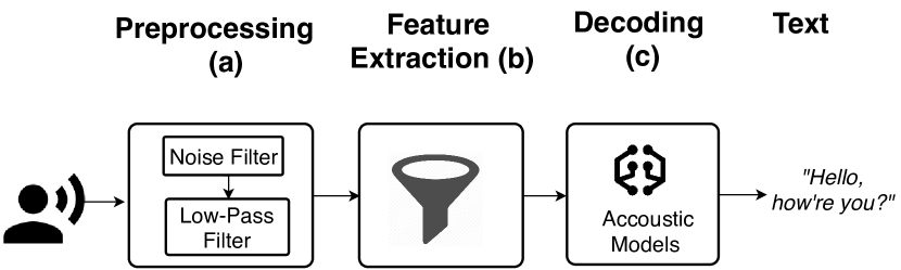
Figure 1: Modern ASR systems take several steps to convert speech into text. (a) Preprocessing removes high frequencies and noise from the audio waveform, (b) feature extraction extracts the most important features of the audio sample, and (c) decoding converts the features into text.

II-A Automatic Speech Recognition (ASR) Systems:

An ASR system converts a sample of speech into text using the steps seen in Figure 1.

(a) Preprocessing Preprocessing in ASR systems attempts to remove noise and interference, yielding a “clean” signal. Generally, this consists of noise filters and low pass filters. Noise filters remove unwanted frequency components from the signal that are not directly related to the speech. The exact process by which the noise is identified and removed varies among different ASR systems. Additionally, since the bulk of frequencies in human speech fall between 300 Hz and 3000Hz [36], discarding higher frequencies with a low pass filter helps remove unnecessary information from the audio.

(b) Feature Extraction Next, the signal is converted into overlapping segments, or frames, each of which is then passed through a feature extraction algorithm. This algorithm retains only the salient information about the frame. A variety of signal processing techniques are used for feature extraction, including Discrete Fourier Transforms (DFT), Mel Frequency Cepstral Coefficients (MFCC), Linear Predictive Coding, and the Perceptual Linear Prediction method [64]. The most common of these is the MFCC method, which is comprised of several steps. First, a magnitude DFT of an audio sample is taken to extract the frequency information. Next, the Mel filter is applied to the magnitude DFT, as it is designed to mimic the human ear. This is followed by taking the logarithm of powers, as the human ear perceives loudness on a logarithmic scale. Lastly, this output is given to the Discrete Cosine Transform (DCT) function that returns the MFCC coefficients.

Some modern ASR systems use data-driven learning techniques to establish which features to extract. Specifically, a machine learning layer (or a completely new model) is trained to learn which features to extract from an audio sample in order to properly transcribe the speech [81].

(c) Decoding During the last phase, the extracted features are passed to a decoding function, often implemented in the form of a machine learning model. This model has been trained to correctly decode a sequence of extracted features into a sequence of characters, phonemes, or words, to form the output transcription. ASR systems employ a variety of statistical models for the decoding step, including Convolutional Neural Networks (CNNs) [66, 17, 55], Recurrent Neural Networks (RNNs) [40, 67, 68, 69], Hidden Markov Models (HMMs) [39, 69], and Gaussian Mixture Models (GMMs) [50, 69]. Each model type provides a unique set of properties and therefore the type of model selected directly affects the ASR system quality. Depending on the model, the extracted features may be re-encoded into a different, learnable feature space before proceeding to the decoding stage. A recent innovation is the paradigm known as end-to-end learning, which combines the entire feature extraction and decoding phase into one model, and greatly simplifies the training process. The most sophisticated methods will leverage many machine learning models during the decoding process. For example, one may employ a dedicated language model, in addition to the decoding function, to improve the ASR’s performance on high-level grammar and rhetorical concepts [20]. Our attacks are agnostic to how the target ASR system is implemented, making our attack completely black-box. To our knowledge, we are the first paper to introduce black-box attacks in a limited query environment.

II-B Automatic Voice Identification (AVI) Systems:

AVI systems are trained to recognize the speaker of a voice sample. The modern AVI pipeline is mostly similar to the one used in the ASR systems, shown in Figure 1. While both systems use the preprocessing and feature extraction steps, the difference lies in the decoding step. Even though the underlying statistical model (i.e., CNNs, RNNs, HMMs or GMMs) at the decoding stage remains the same for both systems, what each model outputs is different. In the case of ASR systems, the decoding step converts the extracted features into a sequence of characters, phonemes, or words, to form the output transcription. In contrast, the decoding step for AVI models outputs a single label which corresponds to an individual. AVI systems are commonly used in security critical domains as an authentication mechanism to verify the identity of a user. In our paper, we present attacks to prevent the AVI models from correctly identifying speakers. To our knowledge, we are the first to do so in a limited query, black-box setting.

II-C Data-Transforms

In this paper, we use standard signal processing transformations to change the representation of audio samples. The transforms can be classified into two categories: data-independent and data-dependent.

II-C1 Data-Independent Transforms

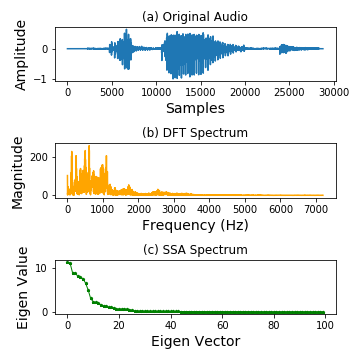
Figure 2: (a) Original audio “about” [1]; (b) the corresponding DFT and (c) SSA decompositions. In both, low magnitude components (frequencies or eigenvectors, respectively) contribute little to the original audio.

These represent input signals in terms of fixed basis functions (e.g., complex exponential functions, cosine functions, wavelets). Different basis functions extract different information about the signal being transformed. For our attack, we focus on the DFT, which exposes frequency information. We do so because the DFT is well understood and commonly used in speech processing, both as a stand-alone tool, and as part of the MFCC method, as discussed in Section II-A.

The DFT, shown in Figure 2(b), represents a discrete-time series $x_{0},x_{1},\ldots,x_{N-1}$ via its frequency spectrum — a sequence of complex values $f_{0},f_{1},\ldots,f_{N-1}$ that are computed as $f_{k}=\sum_{n=0}^{N-1}x_{n}\exp\left((-j2\pi)\frac{k}{N}n\right)$ where $j=\sqrt{-1}$, for $k=0,1,\ldots,N-1$. One can view $f_{k}$ as the projection of the time series onto the $k$-th basis function, a (discrete-time) complex sinusoid with frequency $k/N$ (i.e., a sinusoid that completes $k$ cycles over a sequence of $N$ evenly spaced samples). Intuitively, the complex-valued $f_{k}$ describes “how much” of the time series $x_{0},x_{1},\ldots,x_{N-1}$ is due to a sinusoidal waveform with frequency $k/N$. It compactly encodes both the magnitude of the $k$-th sinusoid’s contribution, as well as phase information, which determines how the $k$-th sinusoid needs to be shifted (in time). The DFT is invertible, meaning that a time-domain signal is uniquely determined by a given sequence of coefficients. Filtering operations (e.g. low-pass/high-pass filters) allow one to accentuate or downplay the contribution of specific frequency components; in the extreme, setting a non-zero $f_{k}$ to zero ensures that the resulting time-domain signal will not contain that frequency.

II-C2 Data-Dependent Transforms

Unlike the DFT, data-dependent transforms do not use predefined basis functions. Instead, the input signal itself determines the effective basis functions: a set of linearly independent vectors which can be used to reconstruct the original input. Abstractly, an input sequence $\mathbf{x}$ with $|\mathbf{x}|=n$ can be thought of as a vector in the space $\mathbb{R}^{n}$, and the data-driven transform finds the bases for the input $\mathbf{x}$. Singular Spectrum Analysis (SSA) is a spectral estimation method that decomposes an arbitrary time series into components called eigenvectors, shown in Figure 2(c). These eigenvectors represent the various trends and noise that make up the original series. Intuitively, eigenvectors corresponding to eigenvalues with smaller magnitudes convey relatively less information about the signal, while those with larger eigenvalues capture important structural information, as long-term “shape” trends, and dominant signal variation from these long-term trends. Similar to the DFT, the SSA is also linear and invertible. Inverting an SSA decomposition after discarding eigenvectors with small eigenvalues is a means to remove noise from the original series.

II-D Cosine Similarity

Cosine Similarity is a metric used to measure the similarity of two vectors. This metric is often used to measure how similar two samples of text are to one another (e.g., as part of the TF-IDF measure [45]). In order to calculate this, the sample texts are converted into a dictionary of vectors. Each index of the vector corresponds to a unique word, and the index value is the number of times the word occurs in the text. The cosine similarity is calculated using the equation $cos(x,y)=\frac{x\cdot y}{||x||\cdot||y||}$, where $x$ and $y$ are the sentence samples. Cosine values close to one mean that the two vectors, or in this case sentences, have high similarity.

II-E Phonemes

Human speech is made up of various component sounds known as phonemes. The set of possible phonemes is fixed due to the anatomy that is used to create them. The number of phonemes that make up a given language varies. English, for example, is made up of 44 phonemes. Phonemes can be divided into several categories depending on how the sound is created. These categories include vowels, fricatives, stops, affricates, nasal, and glides. In this paper, we mostly deal with fricatives and vowels; however, for completeness, will briefly discuss the other categories here.

Vowels are created by positioning the tongue and jaw such that two resonance chambers are created within the vocal tract. These resonance chambers create certain frequencies, known as formants, with much greater amplitudes than others. The relationship between the formants determines which vowel is heard. Examples of vowels include $iy$, $ey$, and $oy$ in the words beet, bait, and boy, respectively.

Fricatives are generated by creating a constriction in the airway that causes turbulent flow to occur. Acoustically, fricatives create a wide range of higher frequencies, generally above 1 kHz, that are all similar in intensity. Common fricatives include the $s$ and $th$ sounds found in words like sea and thin.

Stops are created by briefly halting air flow in the vocal tract before releasing it. Common stops in English include $b$, $g$, and $t$ found in the words bee, gap, and tea. Stops generally create a short section of silence in the waveform before a rapid increase in amplitude over a wide range of frequencies.

Affricates are created by concatenating a stop with a fricative. This results in a spectral signature that is similar to a fricative. English only contains two affricates, $jh$ and $ch$ which can be heard in the words joke and chase, respectively.

Nasal phonemes are created by forcing air through the nasal cavity. Generally, nasals have less amplitude than other phonemes and consist predominantly of lower frequencies. English nasals include $n$ and $m$ such as in the words noon and mom.

Glides are unlike other phonemes, since they are not grouped by their means of production, but instead by their roll in speech. Glides are acoustically similar to vowels but are instead used like consonants, acting as transitions between different phonemes. Examples of glides include the $l$ and $y$ sounds in lay and yes.

III Methodology

III-A Hypothesis and Threat Model

Hypothesis: Our central hypothesis is that ASR and AVI systems rely on components of speech that are non-essential for human comprehension. Removal of these components can dramatically reduce the accuracy of ASR system transcriptions and AVI system identifications without significant loss of audio clarity. Our methods and experiments are designed to test this hypothesis.

Threat Model and Assumptions: For the purposes of this paper, we define the attacker or adversary as a person who is aiming to trick an ASR or AVI system via audio perturbations. In contrast, we define the defender as the owner of the target system.

We assume the attacker has no knowledge of the type, weights, architecture, or layers of the target ASR or AVI system. Thus, we treat each system as a black-box to which we make requests and receive responses. We also assume the attacker can only make a limited number of queries to the target model, as a large number of queries will alert the defender of the attacker’s activities. Furthermore, the attacker has less computational resources than the defender.

We assume the defender has the ability to train an ASR or AVI system. Additionally, they may use any type of machine learning model, feature extraction, or preprocessing to create their ASR or AVI system. Finally, the defender is able to monitor incoming queries to their system and prevent attackers from performing large numbers of queries.

III-B Attack Steps

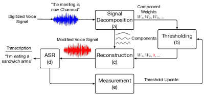
Figure 3: The figure shows the steps involved in generating an attack audio sample. First, the target audio sample is passed through a signal decomposition function (a) which breaks the input signal into components. Next, subject to some constraints, a subset of the components are discarded during thresholding (b). A perturbed audio sample is reconstructed (c) using the remaining weights from (a) and (b) . The audio sample is then passed to the ASR/AVI system (d) for transcription. The difference between the transcription of the perturbed audio and the original audio is measured (e). The thresholding constraints are updated accordingly (c) and the entire process is repeated.

Readers might incorrectly assume that certain trivial attacks might be able to achieve the goals of the dissident i.e., evade the model while maintaining high audio quality. One such trivial attack includes adding white-noise to the speech samples, expecting a mistranscription by the model. However, such a an attack will fail. We discuss in detail how we test this trivial attack and the corresponding results in Appendix A-A. Similarly we introduce a simple impulse perturbation technique that exposes the sensitivity of ASR systems, discussed in Appendix A-B1. Realizing the limitations of this approach, we leave its details to Appendix A-B1 to A-B4. We continue our study to develop a more robust attack algorithm in the following sections.

The attack should meet certain constraints: First, it should introduce artificial noise to the audio sample that exploits the ASR/AVI system and forces an incorrect model output. Second, the distortion should have little to no impact on the understandability of the perturbed audio file for the human listener.

The attack steps are outlined in Figure 3. During decomposition, shown in Figure 3(a), we pass the audio sample to the selected algorithm (DFT or SSA). The algorithm decomposes the audio into individual components and their corresponding intensities. Next, we threshold these components, as shown in Figure 3(b). During thresholding, we remove the components whose intensity falls below a certain threshold. The intuition for doing so is that the lower intensity components are less perceptible to the human ear and will likely not affect a user’s ability to understand the audio. We discuss how the algorithm calculates the correct threshold in the next paragraph. We then construct a new audio sample from the remaining components, using the appropriate inverse transform, shown in Figure 3(c). Next, the audio is passed on to the model for inference, Figure 3(d). If the system being attacked is an ASR, then the model outputs a transcription. On the other hand if the target system is an AVI, the model outputs a speaker label. The model output is compared with that of the original during the measurement step, Figure 3(e).

The goal of the algorithm is to calculate the optimum threshold, which discards the least number of components whilst still forcing the model to misinterpret the audio sample. Discarding components degrades the quality of the reconstructed audio sample. If the discard threshold is too high, neither the human listener nor the model will be able to correctly interpret the reconstructed audio. On the other hand, by setting it too low, both the human listener and the model will correctly understand the reconstructed audio.

To compensate for these competing tensions, the attack algorithm executes the following steps. If the model output matches the original label, during the measurement step, the algorithm will increase the threshold value. It will then pass the audio sample and the updated threshold back to the thresholding step for an additional round of optimization. However, if the model outputs an incorrect interpretation of the audio sample, the algorithm reduces the degradation by reducing the discard threshold, before returning the audio to the thresholding step. This loop will repeat until the algorithm has calculated the optimum discard threshold.

III-C Performance

In order to find the optimal threshold, we incrementally remove more components until the model fails to properly transcribe the audio file. This process takes $O(n)$ queries to the model, where $n$ is the number of decomposition components. We can reduce the time complexity from linear to logarithmic time such that an attack audio is produced in $O(\log~{}n)$ queries. To achieve this, we model the distortion search as a binary search (BS) problem where values represent the number of coefficients to use during reconstruction.

If the reconstruction is misclassified, we move to the left BS search-space and attempt to improve the audio quality by removing less coefficients. If the audio is correctly transcribed, we move to the right. This search continues until either an upper bound on the search depth is reached. This result was sufficient for the scope of this paper, and we leave a more rigorous analysis of distortion search complexity for future work.

III-D Transferability

One measure of an attack’s strength is the ability to generate adversarial examples that are transferable to other models (i.e., a single audio sample that is mistranscribed/misidentified by multiple models). An attacker will not know the precise model he is trying to fool. In such a scenario, the attacker will generate examples for a known model, and hope that the samples will work against a completely different model.

Attacks have been shown to generalize between models in the image domain [59]. In contrast, attack audio transferability has only has seen limited success. Additionally, audio generated with previous approaches ([28, 30]) are sensitive to naturally occurring external noise, which fails to exploit the target model in a real-world setting. This is in line with previous results of physical attacks in the image domain [52]. Instead we focus on the evasion style of attack, where the attack is considered successful if the ASR system transcribes the attack audio incorrectly or the AVI misidentifies the speaker of the attack audio. We propose a completely black-box approach that does not consider model specifics as a means of bypassing these limitations.

III-E Detection and Defense

We evaluate our attack against the adversarial audio detection mechanism which is based on temporal dependencies [82]. This is the only method designed specifically to detect adversarial audio samples. This method has demonstrated excellent results: it is light-weight, simple and highly effective at detecting tradition adversarial attacks. The mechanism takes as input an audio sample. This can either be adversarial or benign. Next, the audio sample is partitioned into two. Only the partition corresponding to the first half is retained. Next, the entire original audio sample and the first partition are passed to the model and the transcriptions are recorded. If the transcriptions are similar, then the audio sample is considered benign. However, if the transcriptions are differing, the audio sample is adversarial. This is because adversarial attack algorithms against audio samples distort the temporal dependence within the original sequences. The temporal dependency-based detection is designed to capture this information and use it for attack audio detection.

Additionally, we evaluate our attack against adversarial training based defense. However, we have placed the steps, the methodology, and the results in the Appendix A-C.

IV Setup

Our experimental setup involved two datasets, four attack scenarios, two test environments, seven target models, and a user study. We discuss the relevant details of our experiments here.

IV-A TIMIT Data Set

The TIMIT corpus is a standard dataset for speech processing systems. It consists of 10 English sentences that are phonetically diverse being spoken by 630 male and female speakers [35]. Additionally, there is metadata of each speaker that includes the speaker’s dialect. In our tests, we randomly sampled six speakers, three male and three female, from each of four regions (New England, Northern, North Midland, and South Midland). We then perturbed all 10 sentences spoken by our speakers using our technique, and also extracted phonemes for our phoneme-level experiments. In total, we attacked 240 recordings with 7600 phonemes.

IV-B Word Audio Data Set

Testing the word-level robustness of an ML model poses challenges in terms of experimental design. Although there exist well-researched datasets of spoken phrases for speech transcription [58, 11], partitioning the phrases into individual words based on noise threshold is not ideal. In this case, the only way to control the distribution of candidate phrases would be to pass them to a strong transcription model, while discarding audio samples which are mistranscribed. Doing so may bias the candidate attack samples towards clean, easy to understand samples. Instead, we build a word-level candidate dataset using a public repository of the 1,000 most common words in the English language [1]. We then download audio for each of the 1,000 words using the Shotooka spoken-word service [9].

IV-C Attack Scenarios

In order to test our technique in a variety of different ways, we performed four attacks: word level, phoneme level, ASR Poisoning, and AVI poisoning. We also tested the transferability of the attack audio samples across models.

IV-C1 Word Level Perturbations

Using the 1,000 most common words, we performed our attack as described in Section III-B. We optimized our threshold using the technique outlined in Section III-D, stopping either after the threshold value had converged or after a maximum of 15 queries.

IV-C2 Phoneme Level Perturbations

Next, we ran perturbations on individual phonemes rather than entire words. The goal of this attack was to cause mistranscription of an entire word by only perturbing a single phoneme. We tested this attack on audio files from the TIMIT corpus and replaced the regular phoneme with its perturbed version in the audio file. The audio sample was then passed to the ASR system for transcription. We repeated this process for every phoneme using the binary search technique outlined in Section III-D.

IV-C3 ASR Poisoning

ASR systems often use the previously transcribed words to infer the transcription of the next [31, 63, 21]. Perturbing a single word’s phonemes not only affects the model’s ability to transcribe that word, but also the words that come after it. We wished to measure the effect of perturbing a single phoneme on the transcription of the remaining words in a sentence. To do this, we generated adversarial audio sample by perturbing a single phoneme while keeping the remaining audio intact for the sentences of the TIMIT dataset. We repeated this for every phoneme in the dataset and passed the attack audio samples to the ASR system. The cosine similarity metric was used to measure the transcription similarity between the attack audio with the original audio.

When perturbing phonemes, we do not use the attack optimization described in Section III-D. Since the average length of a phoneme in our dataset was only 31ms, a single perturbed phoneme in a sentence does not significantly impact audio comprehension. Therefore, we simply discard half of all decomposition coefficients in a single 31 ms window during the thresholding step. This maintains the quality of the adversarial audio, while still forcing the model to mistranscribe.

IV-C4 AVI Poisoning

We also evaluate our attacks’ performance against AVI system. To do so, we first trained an Azure Speaker Identification model [2] to recognize 20 speakers. We selected 10 male and 10 female speakers from the TIMIT dataset to service as our subjects. For each speaker, seven sentences were used for training, while the remaining three sentences were used for attack evaluation. We only perturbed a single phoneme while the rest of the sentence is left unaltered. We passed both the benign and adversarial audio samples to the model. The attack was considered a success if the AVI model output different labels for each sample. This attack setup is similar to the one for ASR poisoning, except that here we target an AVI system.

IV-D Models

We choose a set of seven models that are representative of the state-of-the-art in ASR and AVI technology, given their high accuracy [15, 14, 5, 33]. These include a mixture of both proprietary and open-source models to expose the utility of our attack. However, all are treated as black-box.

Google (Normal): To demonstrate our attack in a truly black-box scenario, we target the speech transcription APIs provided by Google. The ‘Normal’ model is provided by Google for ‘clean’ use cases, such as in home assistants, where the speech is not expected to traverse a cellular network [4].

Google (Phone): To demonstrate our attack against model trained for noisy audio, we test the attack against the ‘Phone’ model. Google provides this model for cellular use cases and trained it on call audio that will be representative of cellular network compression [12]. We also assume that the Google ‘Phone’ model will be robust against the noise, jitter, loss and compression introduced to audio samples that have traveled through the telephony network.

Facebook Wit: To ensure better coverage across the space of proprietary speech transcription services, we also target Facebook Wit, which provides access to a ‘clean’ speech transcription model [16]. As before, no information is known about this model due to its proprietary nature.

Deep Speech-1: The goal of Deep Speech 1 was to eliminate hand-crafted feature pipelines by leveraging a paradigm known as end-to-end learning [39, 41]. This results in robust speech transcription despite noisy environments, if sufficient training data is provided. For our experiments, we use an open-source implementation and checkpoint provided by Mozilla with MFCC features [7].

Deep Speech-2: Deep Speech-2 introduced architecture optimizations for very large training sets. It is trained to map raw audio spectrograms to their correct transcriptions, and demonstrates the current state-of-the-art in noisy, end-to-end audio transcription [20]. We use an open-source implementation trained on LibriSpeech provided by GitHub user SeanNaren [58, 56]. The primary difference in our two tested versions is feature preprocessing: the tested version of Deep Speech-1 uses MFCC features, while the tested version of Deep Speech-2 uses raw audio spectrograms.

CMU Sphinx: The CMU Sphinx project is an open-source speech transcription repository representing over twenty years of research in this task [50]. Sphinx does not heavily rely on deep learning techniques, and instead implements a combination of statistical methods to model speech transcription and high-level language concepts. We use the PocketSphinx implementation and checkpoints provided by the CMU Sphinx repository [50].

Microsoft Azure: To demonstrate our attack against AVI systems in a black-box environment, we attack the Speaker Identification API provided by Microsoft Azure [2]. This system is proprietary, and hence, completely black-box. There is no publicly available information about the internals of the system.

Although the landscape of audio models is ever-changing, we believe our selection represents an accurate approximation of both traditional and state-of-the-art methods. Intuitively, future models will derive from the existing state-of-the-art in terms of data and implementation. We also compare against open-source and proprietary models, to show our approach generalizes to any model regardless of a lack in apriori knowledge.

IV-E Transferability

We measure the transferability of our proposed attack by finding the probability that the attack samples for one model will successfully exploit another. This is done by creating a set of successful word-level attack audio samples $X^{*}_{m}$ for a model $m$, then averaging their calculated Mean Squared Error (MSE) distortion, $\mkern 1.5mu\overline{\mkern-1.5muMSE_{m}\mkern-1.5mu}\mkern 1.5mu$. Intuitively, this average MSE will be higher for stronger models, and lower for weaker models. This acts as a ‘hardness score’ for a given model and is used to compare between attack audio sets of two models. Now consider a baseline model $f$, comparison model $g$, the successful attack transfer event $S_{f\rightarrow g}$, and the number of audio samples in each model’s attack audio set $n=|X^{*}_{f}|=|X^{*}_{g}|$. We can calculate attack transfer probability from $f$ to $g$ as the probability of sampling attack audio from $X^{*}_{f}$ whose distortion meets or surpasses the score $\mkern 1.5mu\overline{\mkern-1.5muMSE_{g}\mkern-1.5mu}\mkern 1.5mu$. We denote this probability $P(S_{f\rightarrow g})$ and the set of potentially transferable audio samples as $V_{f\rightarrow g}$. We calculate the probability using the equation $P(S_{f\rightarrow g})=\frac{|V_{f\rightarrow g}|}{n}$, where we build the set of transferable attack samples such that $V_{f\rightarrow g}=\{\textbf{x}^{*}_{f,i}\in X^{*}_{f}:MSE(\textbf{x}^{*}_{f,i})\geq\mkern 1.5mu\overline{\mkern-1.5mu{MSE}_{g}\mkern-1.5mu}\mkern 1.5mu\}$.

Thus, we approximate the probability of sampling a piece of audio which meets the ‘hardness’ of model $g$ from the set which was successful over model $f$. This value is calculated across each combination of models in our experiments for SSA and DFT transforms, with $n$ set to 1,000 as a result of using our Word Audio data set.

IV-F Detection

Our experimental method was designed to be as close to that of the authors [82]. We assume that the attacker is not aware of the existence of the defense mechanism or the size of the partition. Therefore, we perturbed the entire audio sample using our attack, to maximally distort the temporal dependencies. Next, we partitioned the audio sample into two halves. We passed both the entire audio sample and the first half to the Google Speech API for transcription. We conducted this experiment with 266 adversarial audio samples generated using the DFT perturbation method at a factor of 0.07. Our set of benign audio samples consisted of 534 benign audio samples. The audio samples for both the benign and adversarial sets were taken from the TIMIT dataset. Similar to the authors, we use Word Error Rate (WER) as a measure of transcription similarity. In line with the authors, we calculate and report the Area Under Curve (AUC) value. AUC values lie between 0.5 and 1. A perfect detector will return an AUC of 1, while a detector that randomly guesses returns an AUC of 0.5.

IV-G Over-Cellular

The Over-Cellular environment simulates a more realistic scenario where an adversary’s attack samples have to travel through a noisy and lossy channel before reaching the target system. Additionally, this environment accurately models one of the most common mediums used for transporting human voice – the telephony network. In our case, we did this by sending the audio through AT&T’s LTE network and the Internet via Twilio [13] to an iPhone 6. The attacker’s audio is likely to be distorted while passing through the cellular network due to jitter, packet loss, and the various codecs used within the network. The intuition for testing in this environment is to ensure that our attacks are robust against these kinds of distortions.

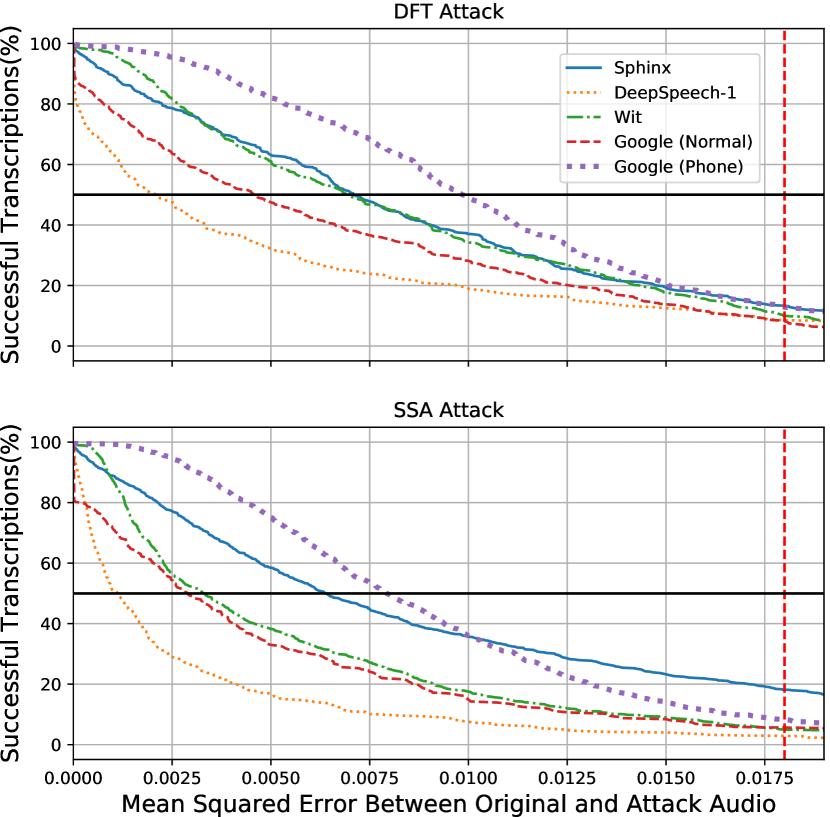
Figure 4: Success transcriptions against our word-level attack plotted against increasing distortion, calculated using Mean Square Error (MSE). The SSA-based word-level attack sees a faster, sharper decrease in the successful transcriptions than the DFT-based word-level attack, noted by its ability to reach 50% attack success (solid black line) across all models within a smaller span of distortion. This means 50% of the words in the dataset were mistrascribed by the target ASR. In every case, the test set accuracy falls considerably before reaching the GSM baseline distortion (dashed red line).

IV-H MTurk Study Design

In order to measure comprehension of perturbed phone call audio, we conducted an IRB approved online study. We ran our study using Amazon’s Mechanical Turk (MTurk) crowdsourcing platform. All participants were between the ages of $18$ and $55$ years old, located in the United States, and had an approval rating for task completion of more than $95\%$. During our study, each participant was asked to listen to audio samples over the phone. Parts of the audio sample had been perturbed, while others had been left unaltered. The audio samples were delivered via an automated phone call to each of our participants. The participants were asked to transcribe the audio of a pre-recorded conversation that was approximately one minute long. After the phone call was done, participants answered several demographic questions which concluded the study. We paid participants $2.00 for completing the task. Participants were not primed about the perturbation of the pre-recorded audio, which prevented introducing any bias during transcription. In order to make our study statistically sound, we ran a sample size calculation under the assumption of following parameter values: an effect size of 0.05, type-I error rate of 0.01, and statistical power of 0.8. Under these given values, our sample size was calculated to be 51 and we ended up recruiting 89 participants in MTurk. Among these 89, 23 participants started but did not complete the study and 5 participants had taken the study twice. After discarding duplicate and incomplete data, our final sample size consists of 61 participants.

V Results

As outlined previously in Section IV-C, we evaluated our attack in various different configurations in order to highlight certain properties of the attack. To begin, we will evaluate our attack against the speech to text capabilities of multiple ASR systems in several different setups.

V-A Attacks Against ASR systems

V-A1 Word Level Perturbations

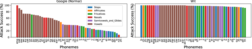
Figure 5: A comparison of attack success of our DFT-based phoneme-level attack against two ASR models. There is a clear relationship between the which phoneme is attacked and the attack’s success. It is clear across all models that we evaluated that vowels are more vulnerable to this attack than other phonemes.

We study the effect of our word-level attack against each model. We measure attack success against distortion and compare the DFT and the SSA attacks, shown in Figure 4. In this subsection, we discuss five target models: Google (Normal), Google (Phone), Wit, DeepSpeech-1 and Sphinx. Distortion is calculated using the MSE between every normal audio sample and its adversarial counterpart.

We use the GSM audio codec’s average MSE as a baseline for audio comprehension, as it is used by 2G cellular networks (the most common globally). We denote this baseline with the red, vertical dashed line in Figure 4. Thus, we consider any audio with higher MSE than the baseline to be totally incomprehensible to humans. It is important to note that this assumption is extremely conservative, since normal comprehensible phone call audio often has larger MSE than our baseline.

Figure 4 shows that as distortion is iteratively increased using the word-level attack, test set accuracy begins to diminish across all models and all transforms. Models which decrease slower, such as Google (Phone), indicate a higher robustness to our attack. In contrast, weaker models, such as Deep Speech-1, exhibit a sharper decline. For all transforms, the Google (Phone) model outperforms the Google (Normal) model. This indicates that training the Google (Phone) model on noisy audio data exhibits a rudimentary form of adversarial training. However, all attacks are eventually successful to at least 85% while retaining audio quality that is comprehensible to humans.

Despite implementing more traditional machine learning techniques, Sphinx exhibits more robustness than Deep Speech-1 across both attacks. This indicates that Deep Speech-1 may be overfitting across certain words or phrases, and its existing architecture is not appropriate for publicly available training data. Due to the black-box nature of Wit and the Google models, it is difficult to compare them directly to their white-box counterparts. Overall, Sphinx is able to match Wit’s performance, which is also more robust than the Google (Normal) model in the DFT attack.

Surprisingly, for the SSA attack Sphinx is able to outperform all models as distortion approaches the human perceptibility baseline. This may be a byproduct of the handcrafted features and models built into Sphinx. Overall, the SSA-based attack manages to induce less distortion, allowing all models to fail with 50% (represented by the horizontal black line) or less test set accuracy before 0.0100 calculated MSE. Manual listening tested showed that there was no perceivable drop in audio quality at this MSE.

V-A2 Phoneme Perturbations

Our evaluation of the phoneme level attacks exposed several trends, as shown in Figures 5 and  12. For brevity, only Google (Normal) and Wit are shown across each data transform, with complete charts available in Section A-D of the Appendix.

Figure 5 shows the relationship between phonemes and attack success. Lower bars correspond to a greater percentage of attack examples that were incorrectly transcribed by the model. According to the figure, vowels are more sensitive to perturbations than other phonemes. This pattern was consistently present across all the models we evaluated. There are a few possible explanations for this behavior. Vowels are the most common phonemes in the English language and their formant frequencies are highly structured. It is possible these two aspects in tandem force the ASR system to over-fit to the specific formant pattern during learning. This would explain why vowel perturbations cause the model to mistranscribe.

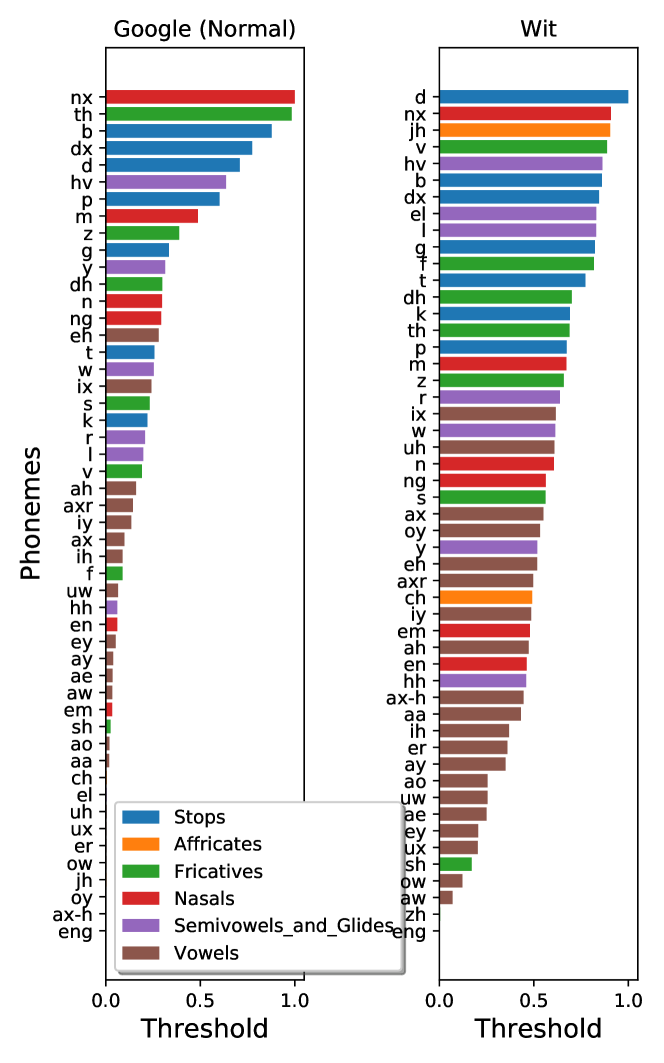
(a) t

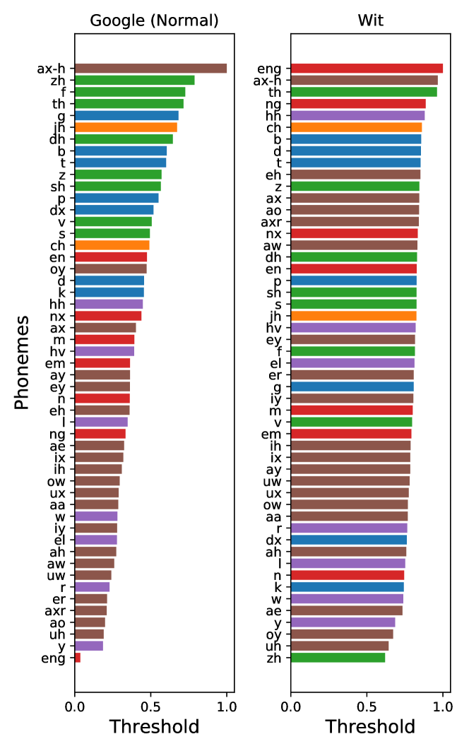
(b) t

Figure 12: Phoneme vulnerability for a selected models, Wit and Google (Normal), using our phoneme-level attacks. Lower threshold corresponds to lower distortion required for an attack success. The DFT attack exhibits a pattern of targeting the vowels (Brown) more effectively than other phonemes. In contrast, the SSA attack does not display any such consistent behavior.

Similarly, Figure 12 shows the distortion thresholds needed for each phoneme to cause mistranscription of a phrase. The longer the bar, the greater the required threshold. For the DFT-based attack experiment, shown in Figure 12(a), we observe that the vowels require a lower threshold compared to the other phonemes. This means that less distortion is required for a vowel to trick the ASR system. In contrast, the SSA-based attack experiments, as shown in Figure 12(b), reveal that all of the phonemes are equally vulnerable. In general, the SSA attacks required a higher threshold than our previous DFT attack. However, the MSE of the audio file after being perturbed when compared to the original audio is still small. The average MSE during these tests was $0.0067$, which is an order of magnitude less than the MSE of audio being sent over LTE ($0.0181$).

Our SSA attacks did not appear to expose any systemic vulnerability in our models as the DFTs did. There exist two likely causes for this: DFT’s use in ASR feature extraction and SSA’s data dependence. ASR systems often use DFTs as part of their feature extraction mechanisms, and thus the models are likely learning some characteristics that are dependent on the DFT. When our attack alters the DFT, we are directly altering acoustic characteristics that will affect which features the model is extracting and learning.

Additionally, when SSA is used in our attack, we are removing eigenvectors rather than specific frequencies like we do with a DFT. These eigenvectors are made up of multiple frequencies that are not unique to any one eigenvector. Thus, the removal of an eigenvector does not guarantee the complete removal of a given frequency from the original audio sample. We believe the combination of these two factors results in our SSA-based attack being equally effective against all phonemes.

Both Figures 5 and 12 provide information for an attacker to maximize their attack success probability. Perturbing vowels at a 0.5 threshold while using a DFT-based attack will provide the highest probability for success because vowels are vulnerable across all models. Even though the discard threshold applied to vowels might vary from one model to another, choosing a threshold value of 0.5 can guarantee both stealth and a high likelihood of a successful mistranscription.

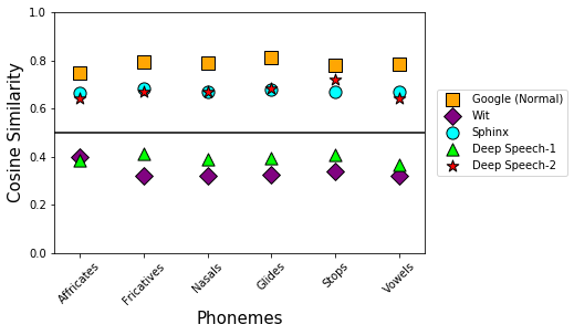
Figure 6: Cosine similarity between the transcriptions of the original and the perturbed audio file. At a value of 0.5 (horizontal line) half of the sentence is incorrect. Attack audio samples were generated by perturbing a single phoneme.

Model	Original Transcription	Attack Transcription
Google (Normal)	The emperor had a mean Temper	syempre Hanuman Temple
	then the chOreographer must arbitrate	Democrat ographer must arbitrate
Wit	she had your dark suit in Greasy wash water all year	nope
	masquerade parties tax one’S imagination	stop

By only perturbing a single phoneme (bold faced and underlined), our attack forces ASR systems to completely mistranscribe the resulting audio.

V-A3 ASR Poisoning

As described in Section IV-C2, perturbing a single phoneme not only causes a mistranscription of the given word but also of the following words as well. Results of this phenomena can be seen in Table V-A2. We further, characterize this numerically across each model for the DFT-based attack in Figure 6, where higher values of cosine similarity translate to lower attack mistranscription.

We observe a relationship between the model type and the cosine similarity score. Of all the models tested, Wit is the most vulnerable, given low average cosine similarity of 0.36. On the other hand, the Google (Normal) model seems to be least vulnerable with the highest cosine similarity of 0.78. To better characterize the phenomenon, we use the cosine similarity value to estimate the number of words that the attack effects. We do so by assuming a sentence comprised of 10 words each. Perturbing a single phoneme can force Wit to mistranscribe the next seven words. In contrast, only two of the next 10 words will be mistranscribed by the Google (Normal) model. This robustness for the Google (Normal) model might be due to its internal recurrent layers being less weighted towards the previously transcribed content. It is also interesting to note that, despite their common internal structure, Deep Speech-1 and Deep Speech-2 are significantly different in their vulnerability to this effect. Deep Speech-1 and Deep Speech-2 have a cosine similarity score of 0.4 and 0.7, respectively. This difference could potentially be attributed to different feature extraction mechanisms. While Deep Speech-1 uses MFCCs, its counterpart uses a CNN feature extraction. This is because feature extraction using MFCCs and CNNs produce varying results and might capture divergent information about the signal.

Observing the models individually, there is no observable relationship between the cosine similarity and the phoneme type. All phonemes seem to be approximately equally vulnerable to the attack. This means that models do not use knowledge of previously occurring phonemes when transcribing the current word. In fact, the results above show that the models use the current phonemes and previous words in combination to transcribe the current word, which intuitively is the intention behind modern ASR system design.

			To (g)
	$P(S_{f\rightarrow g})$	Google (Phone)	Google (Normal)	Wit	Sphinx	Deep-Speech 1
	Google (Phone)	100%	78%	83%	42%	87%
	Google (Normal)	13%	100%	65%	22%	70%
From (f)	Wit	6%	10%	100%	14%	52%
	Sphinx	21%	74%	81%	100%	80%
	Deep-Speech 1	3%	7%	31%	12%	100%

TABLE I: The probability of transferability $P(S_{f\rightarrow g})$ calculated for each combination of the tested models. Only ‘harder’ models tend to transfer well to weaker models. The elements in bold show the highest transferability successes. Model names in the columns have been arranged in descending order of their strength from harder to weaker.

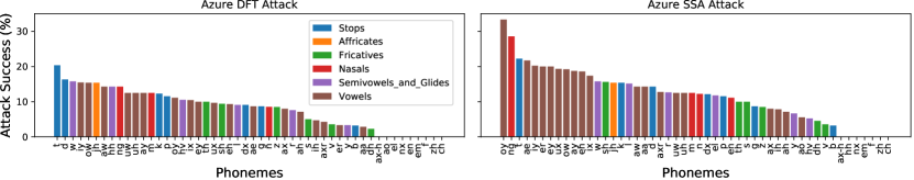
Figure 7: Success rate of our attack against a Automatic Voice Identification (AVI) system. When perturbing a single phoneme in the entire audio sample, an adversary has a greater chance of succeeding with an SSA attack rather than a DFT attack. Additionally, similar to the observation in Figure 5 vowels are more vulnerable than other phonemes.

V-B Attacks Against AVI systems

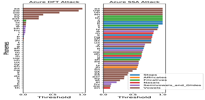
Figure 11: The graph above shows the attacks against a voice identification model. It shows the minimum threshold value required, when perturbing only a single phoneme, to successfully force the model to mis-classify the speaker. We can observe that in general, SSA attacks require much higher thresholds to successfully fool the model, in comparison to the DFT attack.

Next, we observe our attacks’ effectiveness inducing errors an AVI system. Figure 7 shows the attack success rate per vowel for both SSA and DFT attacks. Similar to our attack results against ASR models, attacks against the AVI system exhibited higher success rate when attacking phoneme. This means an adversary wishing to maximize attack success should focus on perturbing vowels. Figure 11 shows the relative amount of perturbation necessary in order to force an AVI misclassification. The SSA attack requires a relatively high perturbation for every phoneme. In contrast, the DFT attack requires a smaller degree of perturbation, all except some vowels. This implies that the DFT attack could be conducted more stealthily by intelligently selecting certain phonemes. The perturbation required, the more stealthy the attack. However, because the SSA attack requires larger degree of perturbations for most phonemes, the level of stealth the attack can achieve is relatively higher.

V-C Transferability

Table I shows results of the transferability experiments using the SSA-based attack. Overall, the attack has the highest transfer probability when a ‘harder’ model is used to generate attack audio samples. The Google (Phone) model had the highest average threshold across samples which, as discussed in Section IV-E, translated to the highest transfer probability. In contrast, a weaker model will have a lower threshold and thus be less likely to transfer. This can be seen when treating Sphinx as the baseline model in Table I. The table shows that in the worst case attack audio generated for the Google (Phone) the model will also be effective against any other model at least 42% of the time. This ensures a high probability of success even in the extreme case when the adversary does not know which model the victim will be employing. By generating attack samples on a stronger model, an adversary can expect an attack to transfer well as long as the victim model is weaker. Finding a weaker model is trivial. As long as the adversary has sufficient queries, they can compare transcription rates for a candidate audio sample between the two models.

V-D Detection

For the detection experiments, we created set of 266 adversarial samples, perturbed using the DFT technique, while the benign set consisted of 534 unperturbed audio samples. Of the adversarial samples provided to the Google Speech API, 20% did not produce any transcription. This was true both the entire audio samples and their corresponding partition. This means that the WER for these samples was 0, which introduced a bias to our results. Though this is perfect for the dissident, but it introduces bias in our results. Specifically, because there are two benign cases in which the WER will be zero, benign audio or very noisy audio. We discarded these audio samples from our adversarial set to remove this bias in our results. In the real world, an attacker can merely reduce the attack factor to prevent the model from producing no transcription. Next, we calculated the AUC scores for the samples. In our case, the AUC value was 0.527, which is far lower than the AUC value of 0.936 reported by the authors for the attacks they tested. This means even though the temporal based detection can do an excellent job of detecting other attacks, it is highly inaccurate for detecting our attack samples.

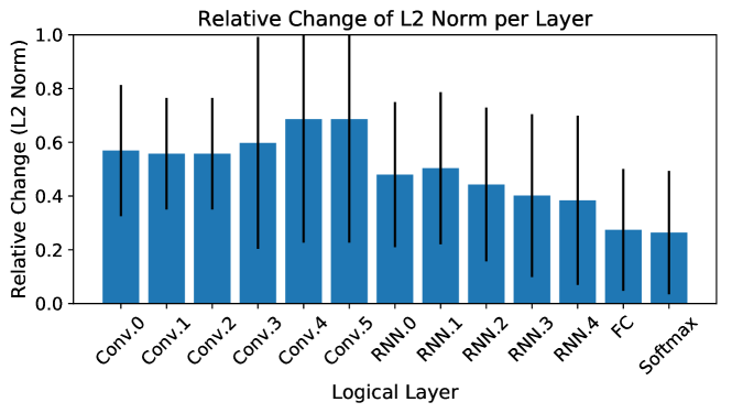
Figure 8: Calculated net change $\Delta h^{l}$ for each layer in the tested Deep Speech 2 model (Convolutional, Recurrent (RNN), fully connected (FC), and Softmax). Lower-level convolutional layers tend to have higher adversarial effect than upper-level recurrent and fully connected layers.

V-E Per-Layer Effects

We now probe more deeply into why the attacks succeed. In particular, we will explore the attacks’ effects at each layer of a typical deep learning-based speech transcription model. We begin by opening our local deployment of Deep Speech-2, which represents a state-of-the-art architecture in this task. The model was provided by an open-source community and was not trained on the same breadth of data as the original proposal [20]. However, examining such a deployment gives insight into the attack’s effects on a publicly available, open-source implementation. We begin by recording the activations at each layer of the Deep Speech-2 architecture for several pairs of original and word-level perturbed audio sample.

We treat the activation of the original audio as a baseline and subtract this from the activation of the perturbed audio to find the net effect. We quantify their distance using the $L_{2}$-norm, then divide this value by the $L_{2}$-norm of the original activation. In total, the tested implementation is comprised of thirteen logical layers, thus for every normal audio $x$, adversarial audio $x^{*}$, layer $h^{l}$, $l\in\{0,...,13\}$, and the $L_{2}$-norm written for brevity as $L_{2}$, we have the layer’s net change $\Delta h^{l}$ calculated using the equation $\Delta h^{l}=\frac{L_{2}[h^{l}(x)-h^{l}(x^{*})]}{L_{2}[h^{l}(x)]}$.

This process was repeated for every benign-perturbed audio pair in our corpus, which is the same corpus built for the word-level perturbation experiments in Section IV-C1. We average across every pair, then repeat this process for every logical layer $h^{l}$ in the Deep Speech-2 architecture to produce the results shown in Figure 8. We observe a higher rate of change for low-level convolutional layers, particularly the upper-level convolutional layers. These convolutional layers learn to mimic and surpass the MFCC preprocessing filter. The net change immediately diminishes as the sample passes through the recurrent layers, reflecting the intuition that changes at individual frames, phonemes, or words may be mitigated by temporal information. However, we also observe a non-zero net change in the fully connected and softmax layers, indicating that the shift was enough to force mistranscription. This points to the CNNs as the main source of the attack vulnerability.

V-F Over-Cellular

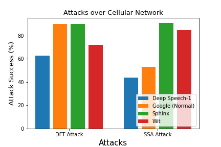
Figure 9: The attack audio was sent over the cellular network and recorded on a mobile end-point. The figure above shows the percentage of the attack audio that was still mistranscribed even after being passed over the cellular network.

Next, we test our attacks for use over a cellular network. We run previously successful attack audio samples over the cellular network before passing them again to the target models. The rate of success for this experiment is shown in Figure 9 plotted against the DFT and SSA-based attacks for each model. If our attack were to be used over a cellular connection, having near real-time performance is important. The largest source of potential delay caused by our attack is from calculating the DFT on the original audio sample. While we do not conduct our own time evaluation, Danielsson et al. showed that calculating a DFT on a commodity Android platform took approximately 0.5 ms for a block size of 4096  [33].

The DFT-based attack managed to be more successful across the mobile network than the SSA-based attack and was only consistently filtered by the Deep Speech and Wit models. Overall, the models react differently based on the transformation. Wit performs best under DFT transforms and worst under SSA transforms, while the opposite is true for Deep Speech 1 and Google (Normal) model. Sphinx is equally vulnerable to both transformation methods.

An intuition for these results can be formed by considering the task each transformation is performing. When transforming with the DFT, the attack audio sample forms around pieces of weighted cross-correlations from the original audio sample. In contrast, the SSA is built as a sum of interpretable principal components. Although SSA may be able to produce fine-grained perturbations to the signal, the granularity of perturbations is lost during the mobile network’s compression. This effect is expected to be amplified for higher amounts of compression, although such a scenario also limits the perceptibility of benign audio.

V-G Amazon Turk Listening Tests

In order to evaluate the transcription done by MTurk workers, we initially manually classified the transcriptions as either correct or incorrect. Table II shows a side by side comparison of original and attack transcription of the perturbed portion of the audio sample. Transcriptions which had either a missing word, a missing sentence, or an additional word not present in the audio were marked as incorrect. At the end of this classification task, the inter-rater agreement value, Cohen’s kappa was found to be $0.901$, which is generally considered to be ‘very good’ agreement among individual raters. Our manual evaluation found only $11\%$ of the transcriptions to be incorrect. More specifically, we found that incorrect transcriptions mostly had missing sentences from the beginning of the played audio sample, but the transcriptions did not contain any misinterpreted words. Our subjective evaluation did not consider wrong transcription of perturbed vs. non-perturbed portion of the audio, rather we only evaluated human comprehension of the audio sample.

In addition to subjective evaluation, we ran a phoneme-level edit distance test on transcriptions to compare the level of transcription accuracy between perturbed and non-perturbed audio samples. We used this formula for phoneme edit distance, $\phi$: $\phi=\frac{\delta}{L}$, where $\delta$ is the Levenshtein edit distance between phonemes of two transcriptions (original transcription and MTurk worker’s transcription) for a word and $L$ is the phoneme length of non-perturbed, normal audio for the word [28]. We defined accuracy as 1 when $\phi=0$, indicating exact match between two transcriptions. For any other value $\phi>0$, we defined it as ‘in-accuracy’ and assigned a value of 0. In Table III, we present transcription accuracy results between perturbed and non-perturbed audio across our final sample size of 61. We also ran a paired sample t-test, using the individual accuracy score for perturbed and benign audio transcriptions, with the null hypothesis that participants’ accuracy levels were similar for both cases of transcriptions. Our results showed participants had better accuracy transcribing non-perturbed audio samples ($mean=0.98,SD=0.13$) than for perturbed audio ($mean=0.90,SD=0.30$). At a significance level of $p<0.01$, our repeated-measures t-test found this difference not to be significant, $t(60)=-2.315,p=0.024$. Recall that our chosen significance level ($p<0.01$) was not arbitrary, rather it was chosen during our sample size calculation for this study. Together, this suggests that our word level audio perturbation create no obstacle for human comprehension in telecommunication tasks, thus supporting our null hypothesis.

Original Transcription	Attack Transcription
How are you? How’s work going?	How are you posmothdro?
I am really sorry to hear that.	I am relief for you to hear that.

TABLE II: Example of the attacked audio which was played to MTurk Workers and the corresponding transcriptions.

Accuracy (Perturbed)		Accuracy (Benign)
Male	Female	Male	Female
91.8% (56/61)	100% (61/61)	98.36% (60/61)	98.36% (60/61)

TABLE III: Transcription accuracy results of MTurk workers for benign and perturbed audios between Male and Female speakers.

VI Discussion

VI-A Phoneme vs. Word Level Perturbation

Our attack aims to force a mistranscription while still being indistinguishable from the original audio to a human listener. Our results indicate that at both the phoneme-level and the word-level, the attack is able to fool black-box models while keeping audio quality intact. However, the choice of performing word-level or phoneme-level attacks is dependent on factors such as attack success guarantee, audible distortion, and speed. The adversary can achieve guaranteed attack success for any word in the dictionary if word-level perturbations are used. However, this is not always true for a phoneme-level perturbation, particularly for phonemes which are phonetically silent. An ASR system may still properly transcribe the entire word even if the chosen phoneme is maximally perturbed. Phoneme-level perturbations may introduce less human-audible distortion to the entire word, as the human brain is well suited to interpolate speech and can compensate for a single perturbed phoneme. In terms of speed, creating word-level perturbations is significantly slower than creating phoneme-level perturbations. This is because a phoneme-level attack requires perturbing only a fraction of the audio samples needed when attacking an entire word.

VI-B Steps to Maximize Attack Success

An adversary wishing to launch an Over-Cellular evasion attack on an ASR system would be best off using the DFT-based phoneme-level attack on vowels, as it guarantees a high level of attack success. Our transferability results show that an attacker can generate samples for a known ‘hard’ model such as Google (Phone) and have reasonable confidence that the attack audio will transfer to an unknown ASR model. From our ASR poisoning results, we observe that an adversary does not have to perturb every word to earn 100% mistranscription of the utterance. Instead, the attacker can perturb a vowel of every other word in the worst case, and every fifth word in the best case. The ASR poisoning effect will ensure that the non-perturbed words are also mistranscribed. Finally, the attack audio samples have a high probability of surviving the compression of a cellular network, which will enable the success of our attack over lossy and noisy mediums.

Contrary to an ASR system attack, an adversary looking to execute an evasion attack on an AVI system would prefer to use the SSA-based phoneme-level attack. Similar to ASR poisoning, we observe that an adversary does not have to perturb the entire sentence to cause a misidentification, but rather just a single phoneme of a word in the sentence. Based on our results, the attacker would need to perturb on average one phoneme every 8 words (33 phoneme) to ensure a high likelihood of attack success. The attack audio samples are generated in an identical manner for both the ASR and AVI system attacks, thus the AVI attack audio should also be robust against lossy and noisy mediums (e.g., a cellular network).

VI-C Why the Attack Works

Our attacks exploit the fundamental difference in how the human brain and ASR/AVI systems process speech. Specifically, our attack discards low intensity components of an audio sample which the human brain is primed to ignore. The remaining components are enough for a human listener to correctly interpret the perturbed audio sample. On the other hand, the ASR or AVI systems have unintentionally learned to depend on these low intensity components for inference. This explains why removing such insignificant parts of speech confuses the model and causes a mistranscription or misidentification. Additionally, this may also explain some portion of the ASR and AVI error on regular testing data sets. Future work may use these revelations in order to build more robust models and be able to explain and reduce ASR and AVI system error.

VI-D Audio CAPTCHAs

In addition to helping dissidents overcome mass-surveillance, our attack has other applications as well. Specifically, in the domain of audio CAPTCHAs. These are often used by web services to validate the presence of a human. CAPTCHAs relies on humans being able to transcribe audio better than machines, an assumption that modern ASR systems call into question [26, 77, 70, 73, 24]. Our attack could potentially be used to intelligently distort audio CAPTCHAs as a countermeasure to modern ASR systems.

VII Related Work

Machine Learning (ML) models, and in particular deep learning models, have shown great performance advancements in previously complex tasks, such as image classification [47, 75, 42] and speech recognition [61, 20, 39]. However, previous work has shown that ML models are inherently vulnerable to a class of ML known as Adversarial Machine Learning (AML) [43].

Early AML techniques focused on visually imperceptible changes to an image that cause the model to incorrectly classify the image. Such attacks target either specific pixels [49, 76, 38, 22, 74, 54], or entire patches of pixels [25, 72, 60, 29]. In some cases, the attack generates entirely new images that the model would classify to an adversary’s chosen target [57, 51].

However, the success of these attacks are a result of two restrictive assumptions. First, the attacks assume that the underlying target model is a form of a neural network. Second, they assume the model can be influenced by changes at the pixel level [60, 57]. These assumptions prevent image attacks from being used against ASR models. ASR systems have found success across a variety of ML architectures, from Hidden Markov Models (HMMs) to Deep Neural Networks (DNNs). Further, since audio data is normally preprocessed for feature extraction before entering the statistical model, the models initially operate at a higher level than the ‘pixel level’ of their image counterparts.

To overcome these limitations, previous works have proposed several new attacks that exploit behaviors of particular models. These attacks can be categorized into three broad techniques that generate audio that include: a) inaudible to the human ear but will be detected by the speech recognition model [84], b) noisy such that it might sound like noise to the human, but will be correctly deciphered by the automatic speech recognition [80, 28, 18], and c) pristine audio such that the audio sounds normal to the human but will be deciphered to a different, chosen phrase [83, 27, 37, 44, 19, 46, 32, 71, 48]. Although they may seem the most useful, attacks in the third category are limited in their success, as they often require white-box access to the model.

Attacks against image recognition models are well studied, giving attackers the ability to execute targeted attacks even in black-box settings. This has not yet been possible against speech models [23], even for untargeted attacks in a query efficient manner. That is, both targeted and untargeted attacks require knowledge of the model internals (such as architecture and parameterization) and large number of queries to the model. In contrast, we propose a query efficient black-box attack that is able to generate an attack audio sample that will be reliably mistranscribed by the model, regardless of architecture or parameterization. Our attack can generate an attack audio sample in logarithmic time, while leaving the audio quality mostly unaffected.

VIII Conclusion

Automatic speech recognition systems are playing an increasingly important role in security decisions. As such, the robustness of these systems (and the foundations upon which they are built) must be rigorously evaluated. We perform such an evaluation in this paper, with particular focus on speech-transcription. By exhibiting black-box attacks against of multiple models, we demonstrate that such systems rely on audio features which are not critical to human comprehension and are therefore vulnerable to mistranscription attacks when such features are removed. We then show that such attacks can be efficiently conducted as perturbations to certain phonemes (e.g., vowels) that cause significantly greater misclassification to the words that follow them. Finally, we not only demonstrate that our attacks can work across models, but also show that the audio generated has no impact on understandability to users. This detail is critical, as attacks that simply obscure audio and make it useless to everyone are not particularly useful to the adversaries we consider. While adversarial training may help in partial mitigations, we believe that more substantial defenses are ultimately required to defend against these attacks.

Appendix A Appendix

We provide additional discussion and results considered insightful, yet tangential to the main contributions of the proposed attack.

Attack Name	Attack Goal	Knowledge	Queries	Telephony	Transferability		Time	Audio Type
					Method	Sample
This Work	Intentional Mistranscription	Black/No	15	✓	✓	✓	milliseconds	Clean
Commander Song [83]	Hiding Signal in Audio	White	?	✗	✓	✗	?	Clean
Qin et al [62]	Hiding Signal in Audio	White	?	✗	✗	✗	?	Clean
Carlini et al. [30]	Hiding Signal in Audio	White	1000	✗	✗	✗	?	Clean
M. Azalnot et al. [19]	Hiding Signal in Audio	Black	?	✗	✓	✗	?	Clean
Houdini [32]	Hiding Signal in Audio	White	?	✗	✗	✗	?	Clean
Schonherr et al. [71]	Hiding Signal in Audio	White	500	✗	✗	✗	minutes	Clean
Skill Squat [48]	Hiding Signal in Audio	Black	?	✗	✗	✗	?	Clean
Kreuk et al. [46]	Hiding Signal in Audio	White	?	✗	✗	✗	?	Clean
Dolphin Attack [84]	Hiding Signal in near Ultrasound	Black	?	✗	✓	✓	?	Inaudible
HVC (1) [28]	Hiding Signal in Noise	White	?	✗	✗	✗	32 hours	Noisy
HVC (2) [28]	Hiding Signal in Noise	Black	?	✗	✗	✗	?	Noisy
Cocaine Noodles [80]	Hiding Signal in Noise	Black	?	✗	✗	✗	?	Noisy
Abdullah et al. [18]	Hiding Signal in Noise	Black	10	✗	✓	✓	seconds	Noisy

TABLE IV: The table provides an overview of the current progress of the adversarial attacks against ASR and AVI systems. The reader can observe that our attack is different from existing works in its attack goal, adversary required knowledge, number of required queries, robustness to the telephony network, transferability, required execution time and the type of audio quality. We have designed the attack to address the specific needs of the dissident, attempting to overcome surveillance infrastructure.
Key: [✗] Won’t work or fails to demonstrate that it will. [✓] Will work. [?] If authors provide no information in paper.

A-A Trivial White-Noise Attack

A-A1 Motivation

Readers might be tempted to use trivial attacks to subvert ASR and AVI models. This includes adding white-noise to benign audio samples. However, in the following subsection, we show that any such trivial techniques will fail to achieve the dissidents’ goals: fool the model whilst not impacting human interpretability of the audio sample.

A-A2 Methodology and Setup

We tested this white-noise method by attacking a random set of 100 audio files that contained speakers uttering a single word. We added white-noise to these samples to generate adversarial audio samples. Next, we passed both the original audio and the white-noise infused audio samples to the Google Speech API. We recorded the number of samples that were incorrectly transcribed by the API.

Next, to measure the impact on human interpretability, we used the Perceptual Evaluation of Speech Quality (PESQ) standard [65]. This is a global standard used for measuring the audio quality of telephony systems. PESQ measures features such as jitter, packet loss, noise and returns a quality score between 1 (bad quality) and 5 (high quality). By using PESQ, supplants the need for user studies to measure audio quality. In our case, the PESQ score can reveal how white-noise will impact audio quality. We calculate the PESQ scores for each of the white-noise infused audio samples and calculated the average.

A-A3 Results

Of the total audio samples we attacked, only 35% of the samples were successfully evaded. Furthermore, average PESQ score for the samples was 1.06, which implies very low audio quality. This proves that any trivial attack will have very low attack success against models, and will have a strong negative impact on human audio interpretability. In contrast, the attack proposed in this paper has little to no impact on the human interpretability (as shown using our Amazon Turk experiments), and achieve 100% success rate against any speech-based models.

A-B Impulse Perturbation Attack

A-B1 Methodology

ASR systems are trained to learn patterns using features from the training set. It is important that training and test sets belong to the same distribution. Otherwise, the model will have difficulty identifying patterns in the test set. Intuitively, we may construct a simple perturbation by sampling outside of the ASR system’s training distribution, then applying it to an input to trick the ASR system.

We extend our study of ASR system’s sensitivity with this extremely simple attack. This involves increasing the amplitude of time-samples within a single phoneme to the maximum amplitude observed in the entire time series. This perturbation will create a minor spike in the audio sample, known as an impulse. If the impulse perturbation succeeds at confusing the model, it will highlight the high sensitivity of the model to artificial perturbations. This will motivate further investigation of other possible attack vectors. These can be designed to confuse the model even further, with limited to no impact on human understandability of the attack audio sample.

The impulse perturbation described above might be able to confuse the model. However, there are a few drawbacks to this approach. First, most popular ASR systems are often trained on both clean and degraded audio quality. This is done to ensure that the ASR systems perform well in noisy environments. Secondly, ASR system’s architecture is designed to ensure that even with a limited training set, the model is able to generalize well. A better generalized model should not be confused by such a simple perturbation. Any simple attack method will only have limited success against ASR systems. Therefore, a further investigation of other attack methods is necessary.

A-B2 Setup

We test our simple attack on the TIMIT corpus. The TIMIT corpus contains the timestamps of each phoneme in the audio file. First, we iteratively selected each phoneme in a word to perturb. Then, each time sample of the target phoneme is replaced with the largest amplitude value in the audio file. Each of the attack audio samples is passed Over-Line to the ASR system for transcription. We then repeat this process, but only perturb one percent of the phoneme. This allows us to identify the relationship between the number of perturbed samples in the phoneme and the mistranscription rate. For brevity, we tested the simple perturbation method against a single model.

A-B3 Results

The simple baseline attack above is executed against the Google (Normal) model. We observe that phonemes with one percent of their samples perturbed only had a 10% attack success rate against the model. This number increases to 43% when the entire phoneme is perturbed by the impulse value. Although the attack has limited success in this scenario, the impulses would likely fail to have an effect against an adversarially-trained model.

A-B4 Simple Defense

During our initial simple perturbation experiments, we observed that applying impulses to individual phonemes was easily distinguishable during manual listening tests. Not only was the attack success rate low, but such impulses were reminiscent of call audio distortions and jitters that are commonly heard over telephony networks. Using this naïve perturbation scheme is not ideal since a machine learning model will likely perform equally well in distinguishing impulses as humans. Overall, adversarial training schemes to defend against this style of attack would be trivial to implement, and do not give an adversary sufficient probability of success under our threat model.

	Original Model	Discard threshold, % of max. DFT coeff.
		2%	4%	8%	16%	32%
Benign Test Set Accuracy (%)	85	78.6	70.2	57.2	47.4	37.8

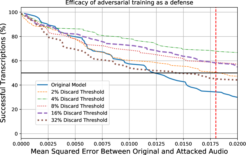
Figure 10: Top: The relationship between the adversarial training and the accuracy of the corresponding model on the benign (unmodified) test set. Bottom: Transcription performance of our (small dictionary) keyword model when trained on audio modified to discard frequencies below various thresholds. The trained models are tested on attack audio with a range of MSE (relative to the corresponding original audio), and the percentage of successful transcriptions are plotted.

A-C Adversarial Training as a Defense:

One technique that has shown promise in defending computer vision models is adversarial training [53]. However, this approach has not seen much success in defending speech and voice identification models [18]. To test this technique against our attack, we trained six keyword recognition models [10]. For each model, we generated adversarial data using the method described Section IV-C1. The threshold was determined as a percentage of the maximum spectral magnitude (i.e., $\max_{k}|f_{k}|$); in particular, we considered 2%, 4%, 8%, 16%, and 32% for each of our models, shown in Figure 10. For example, if the threshold is 4%, we only retain the $f_{k}$ whose magnitude is greater than 4% of the maximum magnitude. Each of the models was trained to detect 10 keywords.

Next, we evaluated each model by randomly selecting 20 samples per keyword. Figure 10 displays the results of our experimentation. Figure 10 (Top) shows the accuracy of each model on the benign data set, while Figure 10 (Bottom) shows the transcription success at various levels of acoustic distortion (relative to the original audio) introduced by our attack. The red dotted line represents the limit of human comprehension as defined earlier in Section V-A1.

There are a few important trends to note. First, models trained with higher threshold values have lower accuracy on normal audio samples, shown in Figure 10 (Top). This result is expected, as lower accuracy is an artifact of adversarial training [79, 34, 49]. Second, as MSE increases, the transcription success rate decreases, shown in Figure 10 (Bottom). The more samples that have lower MSE behind the red dotted GSM line, the more sensitive the model is to our attack. Lastly, adversarial training does decrease model sensitivity to our attack, relative to the baseline model. Intuitively, this implies a relationship between the amount of adversarial training and the minimum amount of distortion caused by our attack.

We caution against taking Figure 10 as strong evidence that adversarial training is a defense against our attack. First, model sensitivity is measured in the number of samples on the left the red GSM line in Figure 10. We used the GSM line as the dividing point between what is and is not comprehensible by human listeners, as discussed in Section V-A. Hence we consider attack audio with MSE values to the right of this line to be failed attack samples. Yet the GSM line should be viewed as a conservative minimum for human comprehension. This is important because, for a given model, our attack may produce many audio samples whose MSE is to the right of the GSM line. Yet, this does not imply that the model is necessarily “robust” against our attack. In particular, some high MSE attack samples may still be understandable by humans while inducing errors in the model. Second, our experimental setup was designed only to support a preliminary investigation of adversarial training as a defense. It would be incorrect to extrapolate any trends from such a simple experiment. A broader and more comprehensive examination should consider (in detail) the effects of different model’s hyper-parameters, and employ a much larger number of audio samples. We leave such a study for future work.

A-D Supplemental Results

References

- [1] “1,000 Most Common US English Words,” Last accessed in 2019, available at https://www.ef.edu/english-resources/english-vocabulary/top-1000-words/.
- [2] “Azure speaker identification api,” Last accessed in 2019, available at https://azure.microsoft.com/en-us/services/cognitive-servic/speaker-recognition/.
- [3] “Background on CTIA’s Semi-Annual Wireless Industry Survey ,” Last accessed in 2019, available at http://files.ctia.org/pdf/CTIA_Survey_YE_2012_Graphics-FINAL.pdf.
- [4] “Google Cloud Speech-to-Text API,” Last accessed in 2019, available at https://cloud.google.com/speech-to-text/.
- [5] “Googles Speech Recognition Technology Now Has a 4.9% Word Error Rate,” Last accessed in 2019, available at https://bit.ly/2rGRtUQ.
- [6] “Inside China’s Massive Surveillance Operation,” Last accessed in 2019, available at https://www.wired.com/story/inside-chinas-massive-surveillance-operation/.
- [7] “Mozilla project deepspeech,” Last accessed in 2019, available at https://azure.microsoft.com/en-us/services/cognitive-servic/speaker-recognition/.
- [8] “NSA Speech Recognition Snowden Searchable Text,” Last accessed in 2019, available at https://theintercept.com/2015/05/05/nsa-speech-recognition-snowden-searchable-text/.
- [9] “Project SHTOOKA - A Multilingual Database of Audio Recordings of Words and Sentences,” Last accessed in 2019, available at http://shtooka.net/.
- [10] “Simple Audio Recognition,” Last accessed in 2019, available at https://www.tensorflow.org/tutorials/sequences/audio_recognition.
- [11] “The CMU Audio Database (also known as AN4 database),” Last accessed in 2019, available at http://www.speech.cs.cmu.edu/databases/an4/.
- [12] “Transcribing Phone Audio with Enhanced Models,” Last accessed in 2019, available at https://cloud.google.com/speech-to-text/docs/phone-model.
- [13] “Twilio - Communication APIs for SMS, Voice, Video and Authentication,” Last accessed in 2019, available at https://www.twilio.com/.
- [14] “Wer are we - an attempt at tracking states of the art(s) and recent results on speech recognition,” https://github.com/syhw/wer_are_we, Last accessed in 2019.
- [15] “Who’s Smartest: Alexa, Siri, and or Google Now?” Last accessed in 2019, available at https://bit.ly/2ScTpX7.
- [16] “Wit.ai Natural Language for Developers,” Last accessed in 2019, available at https://wit.ai/.
- [17] O. Abdel-Hamid, A.-r. Mohamed, H. Jiang, and G. Penn, “Applying convolutional neural networks concepts to hybrid nn-hmm model for speech recognition,” pp. 4277–4280, 05 2012.
- [18] H. Abdullah, W. Garcia, C. Peeters, P. Traynor, K. Butler, and J. Wilson, “Practical hidden voice attacks against speech and speaker recognition systems,” Proceedings of the 2019 Network and Distributed System Security Symposium (NDSS), 2019.
- [19] M. Alzantot, B. Balaji, and M. Srivastava, “Did you hear that? adversarial examples against automatic speech recognition,” arXiv preprint arXiv:1801.00554, 2018.
- [20] D. Amodei et al., “Deep speech 2 : End-to-end speech recognition in english and mandarin,” in Proceedings of The 33rd International Conference on Machine Learning, ser. Proceedings of Machine Learning Research, M. F. Balcan and K. Q. Weinberger, Eds., vol. 48. New York, New York, USA: PMLR, 20–22 Jun 2016, pp. 173–182. [Online]. Available: http://proceedings.mlr.press/v48/amodei16.html
- [21] D. Bahdanau, J. Chorowski, D. Serdyuk, P. Brakel, and Y. Bengio, “End-to-end attention-based large vocabulary speech recognition,” in Acoustics, Speech and Signal Processing (ICASSP), 2016 IEEE International Conference on. IEEE, 2016, pp. 4945–4949.
- [22] S. Baluja and I. Fischer, “Adversarial transformation networks: Learning to generate adversarial examples,” arXiv preprint arXiv:1703.09387, 2017.
- [23] M. K. Bispham, I. Agrafiotis, and M. Goldsmith, “A Taxonomy of Attacks via the Speech Interface,” 2018.
- [24] K. Bock, D. Patel, G. Hughey, and D. Levin, “uncaptcha: a low-resource defeat of recaptcha’s audio challenge,” in Proceedings of the 11th USENIX Conference on Offensive Technologies. USENIX Association, 2017, pp. 7–7.
- [25] T. B. Brown, D. Mané, A. Roy, M. Abadi, and J. Gilmer, “Adversarial patch,” arXiv preprint arXiv:1712.09665, 2017.
- [26] E. Bursztein, R. Beauxis, H. Paskov, D. Perito, C. Fabry, and J. Mitchell, “The failure of noise-based non-continuous audio captchas,” in Security and Privacy (SP), 2011 IEEE Symposium on. IEEE, 2011, pp. 19–31.
- [27] W. Cai, A. Doshi, and R. Valle, “Attacking speaker recognition with deep generative models,” arXiv preprint arXiv:1801.02384, 2018.
- [28] N. Carlini, P. Mishra, T. Vaidya, Y. Zhang, M. Sherr, C. Shields, D. Wagner, and W. Zhou, “Hidden voice commands.” in USENIX Security Symposium, 2016, pp. 513–530.
- [29] N. Carlini and D. Wagner, “Towards evaluating the robustness of neural networks,” in Security and Privacy (SP), 2017 IEEE Symposium on. IEEE, 2017, pp. 39–57.
- [30] N. Carlini and D. Wagner, “Audio Adversarial Examples: Targeted Attacks on Speech-to-Text,” ArXiv e-prints, p. arXiv:1801.01944, Jan. 2018.
- [31] J. K. Chorowski, D. Bahdanau, D. Serdyuk, K. Cho, and Y. Bengio, “Attention-based models for speech recognition,” in Advances in neural information processing systems, 2015, pp. 577–585.
- [32] M. Cisse, Y. Adi, N. Neverova, and J. Keshet, “Houdini: Fooling deep structured prediction models,” arXiv preprint arXiv:1707.05373, 2017.
- [33] A. Danielsson, “Comparing android runtime with native: Fast fourier transform on android,” 2017, mS thesis. [Online]. Available: "https://bit.ly/2MQpUV1"
- [34] E. Dohmatob, “Limitations of adversarial robustness: strong no free lunch theorem,” arXiv preprint arXiv:1810.04065, 2018.
- [35] J. S. Garofolo et al., “Getting started with the darpa timit cd-rom: An acoustic phonetic continuous speech database,” National Institute of Standards and Technology (NIST), Gaithersburgh, MD, vol. 107, p. 16, 1988.
- [36] S. A. Gelfand, Hearing: An Introduction to Psychological and Physiological Acoustics, 5th ed. Informa Healthcare, 2009.
- [37] Y. Gong and C. Poellabauer, “Crafting adversarial examples for speech paralinguistics applications,” arXiv preprint arXiv:1711.03280, 2017.
- [38] I. J. Goodfellow, J. Shlens, and C. Szegedy, “Explaining and harnessing adversarial examples,” arXiv preprint arXiv:1412.6572, 2014.
- [39] A. Graves and N. Jaitly, “Towards end-to-end speech recognition with recurrent neural networks,” in International Conference on Machine Learning, 2014, pp. 1764–1772.
- [40] A. Graves, A.-r. Mohamed, and G. Hinton, “Speech recognition with deep recurrent neural networks,” ICASSP, IEEE International Conference on Acoustics, Speech and Signal Processing - Proceedings, vol. 38, 03 2013.
- [41] A. Hannun, C. Case, J. Casper, B. Catanzaro, G. Diamos, E. Elsen, R. Prenger, S. Satheesh, S. Sengupta, A. Coates et al., “Deep speech: Scaling up end-to-end speech recognition,” arXiv preprint arXiv:1412.5567, 2014.
- [42] K. He, X. Zhang, S. Ren, and J. Sun, “Deep Residual Learning for Image Recognition,” in Proceedings of the IEEE conference on computer vision and pattern recognition, 2016, pp. 770–778.
- [43] L. Huang, A. D. Joseph, B. Nelson, B. I. Rubinstein, and J. D. Tygar, “Adversarial machine learning,” in Proceedings of the 4th ACM Workshop on Security and Artificial Intelligence, ser. AISec ’11. New York, NY, USA: ACM, 2011, pp. 43–58. [Online]. Available: http://doi.acm.org/10.1145/2046684.2046692
- [44] C. Kereliuk, B. L. Sturm, and J. Larsen, “Deep learning and music adversaries,” IEEE Transactions on Multimedia, vol. 17, no. 11, pp. 2059–2071, 2015.
- [45] H. Köpcke, A. Thor, and E. Rahm, “Evaluation of entity resolution approaches on real-world match problems,” Proceedings of the VLDB Endowment, vol. 3, no. 1-2, pp. 484–493, 2010.
- [46] F. Kreuk, Y. Adi, M. Cisse, and J. Keshet, “Fooling end-to-end speaker verification by adversarial examples,” arXiv preprint arXiv:1801.03339, 2018.
- [47] A. Krizhevsky, I. Sutskever, and G. E. Hinton, “Imagenet classification with deep convolutional neural networks,” Neural Information Processing Systems, vol. 25, 01 2012.
- [48] D. Kumar, R. Paccagnella, P. Murley, E. Hennenfent, J. Mason, A. Bates, and M. Bailey, “Skill squatting attacks on amazon alexa,” in 27th USENIX Security Symposium (USENIX Security 18). USENIX Association, 2018.
- [49] A. Kurakin, I. Goodfellow, and S. Bengio, “Adversarial examples in the physical world,” arXiv preprint arXiv:1607.02533, 2016.
- [50] P. Lamere, P. Kwok, W. Walker, E. Gouvêa, R. Singh, B. Raj, and P. Wolf, “Design of the cmu sphinx-4 decoder,” in Eighth European Conference on Speech Communication and Technology, 2003.
- [51] Y. Liu, S. Ma, Y. Aafer, W.-C. Lee, J. Zhai, W. Wang, and X. Zhang, “Trojaning attack on neural networks,” Proceedings of the 2017 Network and Distributed System Security Symposium (NDSS), 2017.
- [52] J. Lu, H. Sibai, E. Fabry, and D. Forsyth, “NO Need to Worry about Adversarial Examples in Object Detection in Autonomous Vehicles,” ArXiv e-prints, 2017.
- [53] A. Madry, A. Makelov, L. Schmidt, D. Tsipras, and A. Vladu, “Towards deep learning models resistant to adversarial attacks,” arXiv preprint arXiv:1706.06083, 2017.
- [54] S. M. Moosavi Dezfooli, A. Fawzi, and P. Frossard, “Deepfool: a simple and accurate method to fool deep neural networks,” in Proceedings of 2016 IEEE Conference on Computer Vision and Pattern Recognition (CVPR), no. EPFL-CONF-218057, 2016.
- [55] T. N. Sainath, A.-r. Mohamed, B. Kingsbury, and B. Ramabhadran, “Deep convolutional neural networks for lvcsr,” pp. 8614–8618, 05 2013.
- [56] S. Naren, “Speech recognition using deepspeech-2,” Last accessed in 2019, available at https://github.com/SeanNaren/deepspeech.pytorch.
- [57] A. Nguyen, J. Yosinski, and J. Clune, “Deep neural networks are easily fooled: High confidence predictions for unrecognizable images,” in Proceedings of the IEEE Conference on Computer Vision and Pattern Recognition, 2015, pp. 427–436.
- [58] V. Panayotov, G. Chen, D. Povey, and S. Khudanpur, “Librispeech: an asr corpus based on public domain audio books,” in Acoustics, Speech and Signal Processing (ICASSP), 2015 IEEE International Conference on. IEEE, 2015, pp. 5206–5210.
- [59] N. Papernot, P. McDaniel, I. Goodfellow, S. Jha, Z. B. Celik, and A. Swami, “Practical Black-box Attacks Against Machine Learning,” in Proceedings of the 2017 ACM on Asia Conference on Computer and Communications Security. ACM, 2017, pp. 506–519.
- [60] N. Papernot, P. McDaniel, S. Jha, M. Fredrikson, Z. B. Celik, and A. Swami, “The limitations of deep learning in adversarial settings,” in Security and Privacy (EuroS&P), 2016 IEEE European Symposium on. IEEE, 2016, pp. 372–387.
- [61] D. Povey, A. Ghoshal, G. Boulianne, L. Burget, O. Glembek, N. Goel, M. Hannemann, P. Motlíček, Y. Qian, P. Schwarz, J. Silovský, G. Stemmer, and K. Veselý, “The kaldi speech recognition toolkit,” in IEEE 2011 Workshop on Automatic Speech Recognition and Understanding. IEEE Signal Processing Society, 2011, iEEE Catalog No.: CFP11SRW-USB.
- [62] Y. Qin, N. Carlini, I. Goodfellow, G. Cottrell, and C. Raffel, “Imperceptible, robust, and targeted adversarial examples for automatic speech recognition,” arXiv preprint arXiv:1903.10346, 2019.
- [63] L. R. Rabiner and B.-H. Juang, Fundamentals of speech recognition. PTR Prentice Hall Englewood Cliffs, 1993, vol. 14.
- [64] L. R. Rabiner and R. W. Schafer, Digital processing of speech signals. Prentice Hall, 1978.
- [65] A. W. Rix, J. G. Beerends, M. P. Hollier, and A. P. Hekstra, “Perceptual evaluation of speech quality (pesq)-a new method for speech quality assessment of telephone networks and codecs,” in 2001 IEEE International Conference on Acoustics, Speech, and Signal Processing. Proceedings (Cat. No. 01CH37221), vol. 2. IEEE, 2001, pp. 749–752.
- [66] T. N. Sainath, O. Vinyals, A. Senior, and H. Sak, “Convolutional, long short-term memory, fully connected deep neural networks,” in 2015 IEEE International Conference on Acoustics, Speech and Signal Processing (ICASSP), April 2015, pp. 4580–4584.
- [67] H. Sak, A. Senior, and F. Beaufays, “Long short-term memory recurrent neural network architectures for large scale acoustic modeling,” Proceedings of the Annual Conference of the International Speech Communication Association, INTERSPEECH, pp. 338–342, 01 2014.
- [68] H. Sak, O. Vinyals, G. Heigold, A. Senior, E. McDermott, R. Monga, and M. Mao, “Sequence discriminative distributed training of long short-term memory recurrent neural networks,” Proceedings of the Annual Conference of the International Speech Communication Association, INTERSPEECH, pp. 1209–1213, 01 2014.
- [69] H. Sak, A. Senior, K. Rao, and F. Beaufays, “Fast and accurate recurrent neural network acoustic models for speech recognition,” CoRR, vol. abs/1507.06947, 2015. [Online]. Available: http://arxiv.org/abs/1507.06947
- [70] S. Sano, T. Otsuka, and H. G. Okuno, “Solving google’s continuous audio captcha with hmm-based automatic speech recognition,” in International Workshop on Security. Springer, 2013, pp. 36–52.
- [71] L. Schönherr, K. Kohls, S. Zeiler, T. Holz, and D. Kolossa, “Adversarial attacks against automatic speech recognition systems via psychoacoustic hiding,” arXiv preprint arXiv:1808.05665, 2018.
- [72] M. Sharif, S. Bhagavatula, L. Bauer, and M. K. Reiter, “Accessorize to a crime: Real and stealthy attacks on state-of-the-art face recognition,” in Proceedings of the 2016 ACM SIGSAC Conference on Computer and Communications Security. ACM, 2016, pp. 1528–1540.
- [73] S. Solanki, G. Krishnan, V. Sampath, and J. Polakis, “In (cyber) space bots can hear you speak: Breaking audio captchas using ots speech recognition,” in Proceedings of the 10th ACM Workshop on Artificial Intelligence and Security. ACM, 2017, pp. 69–80.
- [74] J. Su, D. V. Vargas, and S. Kouichi, “One pixel attack for fooling deep neural networks,” arXiv preprint arXiv:1710.08864, 2017.
- [75] C. Szegedy, W. Liu, Y. Jia, P. Sermanet, S. Reed, D. Anguelov, D. Erhan, V. Vanhoucke, and A. Rabinovich, “Going Deeper with Convolutions,” in 2015 IEEE Conference on Computer Vision and Pattern Recognition (CVPR), June 2015, pp. 1–9.
- [76] C. Szegedy, W. Zaremba, I. Sutskever, J. Bruna, D. Erhan, I. Goodfellow, and R. Fergus, “Intriguing properties of neural networks,” arXiv preprint arXiv:1312.6199, 2013.
- [77] J. Tam, J. Simsa, S. Hyde, and L. V. Ahn, “Breaking audio captchas,” in Advances in Neural Information Processing Systems, 2009, pp. 1625–1632.
- [78] R. Taori, A. Kamsetty, B. Chu, and N. Vemuri, “Targeted adversarial examples for black box audio systems,” arXiv preprint arXiv:1805.07820, 2018.
- [79] D. Tsipras, S. Santurkar, L. Engstrom, A. Turner, and A. Madry, “Robustness may be at odds with accuracy,” arXiv preprint arXiv:1805.12152, vol. 1, 2018.
- [80] T. Vaidya, Y. Zhang, M. Sherr, and C. Shields, “Cocaine noodles: exploiting the gap between human and machine speech recognition,” WOOT, vol. 15, pp. 10–11, 2015.
- [81] S. Venugopalan, H. Xu, J. Donahue, M. Rohrbach, R. Mooney, and K. Saenko, “Translating videos to natural language using deep recurrent neural networks,” arXiv preprint arXiv:1412.4729, 2014.
- [82] Z. Yang, B. Li, P.-Y. Chen, and D. Song, “Characterizing audio adversarial examples using temporal dependency,” arXiv preprint arXiv:1809.10875, 2018.
- [83] X. Yuan, Y. Chen, Y. Zhao, Y. Long, X. Liu, K. Chen, S. Zhang, H. Huang, X. Wang, and C. A. Gunter, “Commandersong: A systematic approach for practical adversarial voice recognition,” in Proceedings of the USENIX Security Symposium, 2018.
- [84] G. Zhang, C. Yan, X. Ji, T. Zhang, T. Zhang, and W. Xu, “Dolphinattack: Inaudible voice commands,” in Proceedings of the 2017 ACM SIGSAC Conference on Computer and Communications Security. ACM, 2017, pp. 103–117.