Power Limit of Crosswind Kites

Abstract

In this paper, a generalized power limit of the cross wind kite energy systems is proposed. Based on the passivity property of the aerodynamic force, the available power which can be harvested by a cross wind kite is derived. For the small side slip angle case, an analytic result is calculated. Furthermore, an algorithm to calculated the real time power limit of the cross wind kites is proposed.

1 Introduction

Crosswind kite power is an emerging renewable energy technology which uses kites or gliders to generate power in high altitude wind flow. Compared to the conventional wind turbine technology, the crosswind power systems can achieve high-speed crosswind motion, which increase the power density significantly. Additionally, without the support structure, the construction cost of such wind energy system could be reduced compared to conventional towered wind turbines. This could eventually reduce the cost of the wind energy dramatically.

Based on the power generation modes, the crosswind power can be placed into two categories: the FlyGen systems and the GroundGen systems. FlyGen systems, also referred to as drag mode systems, generate power through on-board devices, such as wind turbine. GroundGen systems, also referred to as lift mode systems, generate power through tether tension and power generator on the ground. Different industrial prototypes have been proposed for the airborne wind harvesting,

Although the theoretical power limit of crosswind kites is the most fundamental issue of such systems. In [1], Miles Loyd first proposed a power limit for the crosswind kite systems. Diehl provide a refined version of the power limit in [2] by considering the turbine power generation. However, both Loyd and Diehl’s works are based on kite motion in a two-dimensional wind field and no side force has been taken into account in their analysis. In this paper, I propose the theoretical limit of the crosswind kite systems in three-dimensional wind field, and the following contributions are made. First, a general power loss of the crosswind kite system is derived based on the passivity analysis of the classical aerodynamic model. Based on the power loss calculation, the available power of a crosswind kite is derived, and a nonlinear optimization is presented to determine the power limit.

2 Available Power

In this section, the available power of the cross wind kites will be derived. First, a classical aerodynamic model is presented and the passivity property of the aerodynamic force is then proven. Physically, the passivity of the aerodynamic force represents the power dissipated by the aerodynamic force. Then available power of the crosswind kite systems is then derived based on this property of the aerodynamic force. The derivation presented in this section serves as a foundation of the power limit calculation of the cross wind kite in next section.

2.1 Classical Model of Aerodynamics

As in classical aerodynamics, [3] the following two reference frames are used to describe the three-dimensional kite motion,

• Cartesian Earth Frame C: $\begin{pmatrix}\mathbf{i}_{C}&\mathbf{j}_{C}&\mathbf{k}_{C}\end{pmatrix}$

• Body Frame B: $\begin{pmatrix}\mathbf{i}_{B}&\mathbf{j}_{B}&\mathbf{k}_{B}\end{pmatrix}$

In crosswind kite systems, the Cartesian earth frame C is often assumed to center at anchor point of the tether. The $\mathbf{i}_{C}$ axis points to the upstream direction and $\mathbf{j}_{C}$ points vertical downwards. The $\mathbf{j}_{C}$ axis forms a right-hand coordinate system with $\mathbf{i}_{C}$ and $\mathbf{k}_{C}$ axes. The body frame B, which centers at the gravitational center of the kite, follows the North-East-Down conventions.

In this work, we will denote the rotational transformation matrix from frame C to B as $\mathbf{L}_{BC}$, which can be represented either by Euler angles or quaternion. The the kite and wind velocity measured in frame C are denoted as $\mathbf{V}_{C}$ and W respectively, then the kite and wind velocity observed in frame B are given by,

$$\mathbf{V}_{B}=\mathbf{L}_{BC}\mathbf{V}_{C},\hskip 10.00002pt\mathbf{W}_{B}=\mathbf{L}_{BC}\mathbf{W}_{C}.$$ (1)

It is well known that the rotational transformation matrices are orthogonal, i.e., it inverse transformation, denoted as $\mathbf{L}_{CB}$, is its transpose,

$$\mathbf{L}_{CB}=\mathbf{L}_{BC}^{-1}=\mathbf{L}_{BC}^{T}.$$ (2)

The kite apparent velocity, which is denoted as $\mathbf{V}_{a}$, is the key in determining the aerodynamic force acting on kites. Using the notation in equations (1) and (2),

$$\mathbf{V}_{a}=\mathbf{L}_{BC}(\mathbf{V}_{C}-\mathbf{W}_{C})=\begin{pmatrix}u_{a}&v_{a}&w_{a}\end{pmatrix},$$ (3)

for convenience, $-\mathbf{V}_{a}$ may also be referred to as apparent wind velocity. Using kite apparent velocity, $\mathbf{V}_{a}$, the kite apparent attitudes, angle of attack $\alpha$ and sideslip angle $\beta$, are given by

$$\alpha=\arctan\big{(}\frac{w_{a}}{u_{a}}\big{)},\hskip 10.00002pt\beta=\arcsin\big{(}\frac{v_{a}}{V_{a}}\big{)},$$ (4)

where $V_{a}=\|\mathbf{V}_{a}\|$ is also refer as the kite apparent speed.

It is a common practice, [3], that the kite apparent velocity in $\mathbf{i}_{B}$ is assumed to be positive, which is clearly state as follows,

Assumption 1.

The kite apparent velocity along $\mathbf{i}_{B}$ direction is positive, i.e. $u_{a}>0$.

In conventional wind energy system, [4], Assumption 1 simply implies that the wind turbine is assumed always facing to the wind during the power harvesting. Under this assumption, the kite apparent velocity $\mathbf{V}_{a}$ can be represented by the apparent attitudes, $\alpha$ and $\beta$, in the following way,

$$\mathbf{V}_{a}=\|\mathbf{V}_{a}\|\begin{pmatrix}\cos\alpha\cos\beta&\sin\beta&\sin\alpha\cos\beta\end{pmatrix}^{T}.$$ (5)

Equation (5) states that the kite apparent velocity is a function of kite apparent attitudes. In classical aerodynamics, kite lift and drag coefficients, $C_{L}$ and $C_{D}$, are also functions of apparent attitudes,

$$C_{L}=C_{L}(\alpha),\hskip 10.00002ptC_{D}=C_{D}(\alpha).$$ (6)

By convention, lift and drag coefficients are defined based on the flow direction, i.e. direction of $V_{\infty}$ shown in Figure 1. The aerodynamic coefficients along the body axes are given by applying appropriate trigonometric transformation,

$$\begin{pmatrix}C_{x}\\ C_{z}\end{pmatrix} =\begin{pmatrix}1&0\\ 0&-1\end{pmatrix}\begin{pmatrix}\sin\alpha&-\cos\alpha\\ \cos\alpha&\sin\alpha\end{pmatrix}\begin{pmatrix}C_{L}\\ C_{D}\end{pmatrix},$$

$$\mathbf{C}_{B} =\begin{pmatrix}C_{x}&C_{y}&C_{z}\end{pmatrix}^{T}-\begin{pmatrix}C_{t}&0&0\end{pmatrix}^{T},$$

where $C_{t}$ is the turbine drag coefficient and $C_{y}$ is the side force coefficient. In a more compact form, the kite aerodynamic coefficient in frame B is given by,

$$\mathbf{C}_{B}=\begin{pmatrix}C_{L}\sin\alpha-C_{D}\cos\alpha-C_{t}\\ C_{y}\\ -C_{L}\cos\alpha-C_{D}\sin\alpha\end{pmatrix}.$$ (7)

Therefore, the steady aerodynamic force acting on the kite, measured in frame B, can be calculated as

$$\mathbf{A}_{B}=\frac{1}{2}\rho SV_{a}^{2}\mathbf{C}_{B},$$ (8)

where $S$ is the kite area and $\rho$ is the air density. Correspondingly, the steady aerodynamic force acting on the kite, measured in frame C, is given by

$$\mathbf{A}_{C}=\frac{1}{2}\rho SV_{a}^{2}\mathbf{L}_{CB}\mathbf{C}_{B},$$ (9)

To this end, all important notations that will be used in the rest of the paper have been introduced. To achieve a more general power limit of crosswind kite, the passivity of the aerodynamic force should be first discussed.

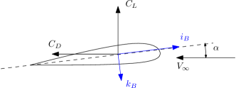
Figure 1: Lift and Drag Coefficients

2.2 Power Loss

To establish the passivity property of the aerodynamic model given in equations (8) and (9), some definitions in nonlinear system theory, [5], need to be reviewed first. Consider a function, $\mathbf{y}=\mathbf{h}(\mathbf{u})$, where $\mathbf{y}$ and $\mathbf{u}$ are input and output signal with compatible dimensions. Then, the passivity of function $\mathbf{h}(\mathbf{u})$ is defined formally as follows,

Definition 1.

A function $\mathbf{y}=\mathbf{h}(\mathbf{u})$ is Passive if $\mathbf{u}^{T}\mathbf{y}\geq 0$. The function is strictly input passive if there exist a function $\boldsymbol{\varphi}(\mathbf{u})$, with proper dimension, such that $\mathbf{u}^{T}\boldsymbol{\varphi}(\mathbf{u})>0$ for all $\mathbf{u}\neq\mathbf{0}$ and $\mathbf{u}^{T}\mathbf{y}\geq\mathbf{u}^{T}\boldsymbol{\varphi}(\mathbf{u})$.

The classical aerodynamics model introduced in the previous section, i.e equations (3) - (8), can be represented using block diagram shown in Figure 2.

Figure 2: Block Diagram of Aerodynamic Model

The kite apparent velocity, $\mathbf{V}_{a}$, can be treated as input to the model while the aerodynamic force in frame B, $\mathbf{A}_{B}$, is the output of the model. Then the following lemma can be proven,

Lemma 1.

Under the Assumption 1, the aerodynamic force is strictly input passive with respect to apparent wind velocity.

$$-\mathbf{V}_{a}^{T}\mathbf{A}_{B}=-\frac{1}{2}\rho\|\mathbf{V}_{a}\|^{3}SC_{a}>0.$$ (10)

where $C_{a}$ is given by,

$$C_{a}=-C_{D}\cos\beta+C_{y}\sin\beta-C_{t}\cos\alpha\cos\beta.$$

Please refer to [6] for detailed proof of this lemma. The passivity of the kite consists of two parts, the power dissipation due to kite structure and the power harvested by the on board turbine. Therefore,

Remark 1.

The pure power loss due to the kite structure is given by,

$$\mathbf{V}_{a}^{T}\mathbf{A}_{k}=\frac{1}{2}\rho\|\mathbf{V}_{a}\|^{3}S\big{(}-C_{D}\cos\beta+C_{y}\sin\beta\big{)},$$ (11)

where $\mathbf{A}_{k}=\mathbf{A}_{B}$ with $C_{t}=0$.

2.3 Available Power of Crosswind Kites

Using the power extraction formula given in [2], the total power that can be extracted from the wind in the kite cross wind motion can be computed as follows,

$$P_{t}=\mathbf{W}_{C}^{T}\mathbf{A}_{C}=\mathbf{W}_{B}^{T}\mathbf{A}_{B}.$$ (12)

The second equality can be derived by using equations (1), (2) and (9). Combining with Remark 1, the available power in a cross wind motion is

$$P_{a}=\mathbf{W}_{B}^{T}\mathbf{A}_{B}+\mathbf{V}_{a}^{T}\mathbf{A}_{k}.$$ (13)

Denote the wind velocity measured in frame B as,

$$\mathbf{W}_{B}=\begin{pmatrix}W_{x}&W_{y}&W_{z}\end{pmatrix}^{T}.$$ (14)

Then by substituting equations (5), (7), (8) and (11) into equation (13), the available power is given by

$$P_{a} =\frac{1}{2}\rho\|\mathbf{V}_{a}\|^{2}S\mathbf{W}_{B}^{T}\mathbf{C}_{B}+\mathbf{V}_{a}^{T}\mathbf{A}_{k}$$

$$=\frac{1}{2}\rho\|\mathbf{V}_{a}\|^{2}S\Big{(}W_{x}(C_{L}\sin\alpha-C_{D}\cos\alpha-C_{t})$$

$$+W_{y}C_{y}-W_{z}(C_{L}\cos\alpha+C_{D}\sin\alpha)$$

$$+\|\mathbf{V}_{a}\|(-C_{D}\cos\beta+C_{y}\sin\beta)\Big{)}.$$ (15)

Hence, it is clear that the theoretical power limit of a crosswind kite system can be computed from the following nonlinear optimization problem,

$$\max_{\alpha,\beta,V_{a}}\hskip 5.0pt \frac{1}{2}\rho S\|\mathbf{V}_{a}\|^{2}\Big{(}W_{x}(C_{L}\sin\alpha-C_{D}\cos\alpha-C_{t})$$

$$+W_{y}C_{y}-W_{z}(C_{L}\cos\alpha+C_{D}\sin\alpha)$$

$$+\|\mathbf{V}_{a}\|(-C_{D}\cos\beta+C_{y}\sin\beta)\Big{)}.$$ (16)

3 Theoretical Power Limits

It worth noting that the available power given in (15) is a nonlinear function of the angle of attack $\alpha$ and side slip angle $\beta$, and the solution to the nonlinear optimization problem (16) is difficult to obtain. However, under certain simplified assumptions, the theoretical power limit of cross wind kite can be computed analytically. In this section, three different theoretical power limits, under three different assumptions, will be derived. First, I will show that the classical Loyd’s limit can be derived by assuming the side force acting on the kite is zero and the turbine drag and kite drag force are co-linear. Then, a power limit that only assuming the side force is zero will be derived. Finally, the power limit, under small side slip angle assumption, will also be derived analytically.

3.1 Loyd’s Limit

In classical aerodynamics, it is reasonable to assume that the side force is negligible when the side slip angle is zero, that is

Assumption 2.

If the side slip angle is zero then the side force coefficient is also zero, i.e.

$$C_{y}=0\hskip 10.00002pt\mbox{if}\hskip 10.00002pt\beta=0$$ (17)

To derive the Loyd’s limit, the following assumptions are also necessary,

Assumption 3.

The kite drag and turbine drag forces are co-linear.

Under the Assumption 3, the aerodynamic coefficients given in (7) can be simplified as follows,

$$\mathbf{C}_{B}=\begin{pmatrix}C_{L}\sin\alpha-(C_{D}+C_{t})\cos\alpha\\ C_{y}\\ -C_{L}\cos\alpha-(C_{D}+C_{t})\sin\alpha\end{pmatrix}.$$ (18)

Therefore, the available power of the kite given in equation (15) can be approximated by

$$P_{a}= \frac{1}{2}\rho S\|\mathbf{V}_{a}\|^{2}\Big{(}W_{x}(C_{L}\sin\alpha-(C_{D}+C_{t})\cos\alpha)$$

$$+W_{y}C_{y}-W_{z}(C_{L}\cos\alpha+(C_{D}+C_{t})\sin\alpha)$$

$$+\|\mathbf{V}_{a}\|(-C_{D}\cos\beta+C_{y}\sin\beta)\Big{)}.$$ (19)

Under the assumptions 2 and 3, the upper bound of the available power can be found as in the following theorem,

Theorem 1.

Assume that the sideslip angle $\beta$ is zero and the kite drag is co-linear with the turbine drag, then the available power of the crosswind kite, with on-board turbine, is bounded by

$$P_{a}\leq\frac{2}{27}\rho S(\sqrt{W_{x}^{2}+W_{z}^{2}})^{3}\frac{(\sqrt{C_{L}^{2}+(C_{D}+C_{t})^{2}})^{3}}{C_{D}^{2}}.$$ (20)

Especially, without on-board turbine, the available power is bounded by

$$P_{a}\leq\frac{2}{27}\rho S(\sqrt{W_{x}^{2}+W_{z}^{2}})^{3}\frac{(\sqrt{C_{L}^{2}+C_{D}^{2}})^{3}}{C_{D}^{2}}.$$ (21)

Proof.

Under the assumption 2, if $\beta=0$ then $C_{y}=0$, and the available power (19) can be simplified as follows,

$$P_{a}= \frac{1}{2}\rho S\|\mathbf{V}_{a}\|^{2}\Big{(}W_{x}(C_{L}\sin\alpha-(C_{D}+C_{t})\cos\alpha)$$

$$- W_{z}(C_{L}\cos\alpha+(C_{D}+C_{t})\sin\alpha)-\|\mathbf{V}_{a}\|C_{D}\Big{)}.$$ (22)

Notice that

$$W_{x}(C_{L}\sin\alpha-(C_{D}+C_{t})\cos\alpha)$$

$$-W_{z}(C_{L}\cos\alpha+(C_{D}+C_{t})\sin\alpha)=(\mathbf{W}_{B}^{{}^{\prime}})^{T}\mathbf{C}_{B}^{{}^{\prime}},$$ (23)

where $\mathbf{W}_{B}^{{}^{\prime}}$ and $\mathbf{C}_{B}^{{}^{\prime}}$ are defined as

$$\mathbf{W}_{B}^{{}^{\prime}} =\begin{pmatrix}W_{x}&W_{z}\end{pmatrix},$$

$$\mathbf{C}_{B}^{{}^{\prime}} =\begin{pmatrix}C_{L}\sin\alpha-(C_{D}+C_{t})\cos\alpha\\ -C_{L}\cos\alpha-(C_{D}+C_{t})\sin\alpha\end{pmatrix}.$$

It is clear that the norm of $\mathbf{C}_{B}^{{}^{\prime}}$ and $\mathbf{W}_{B}^{{}^{\prime}}$ are given by

$$\|\mathbf{C}_{B}^{{}^{\prime}}\|= \sqrt{C_{L}^{2}+(C_{D}+C_{t})^{2}}$$

$$\|\mathbf{W}_{B}^{{}^{\prime}}\|= \sqrt{W_{x}^{2}+W_{z}^{2}}$$

Therefore the upper bound of the available power $P_{a}$ is

$$P_{a}\leq \frac{1}{2}\rho S\|\mathbf{V}_{a}\|^{2}\Big{(}\sqrt{W_{x}^{2}+W_{z}^{2}}\sqrt{C_{L}^{2}+(C_{D}+C_{t})^{2}}$$

$$-\|\mathbf{V}_{a}\|C_{D}\Big{)}.$$ (24)

Differentiating the right hand side of (24) with respect to $\|\mathbf{V}_{a}\|$ gives,

$$\frac{\partial}{\partial\|\mathbf{V}_{a}\|}\bigg{(}\|\mathbf{V}_{a}\|^{2}\Big{(}\|\mathbf{W}_{B}^{{}^{\prime}}\|\sqrt{C_{L}^{2}+(C_{D}+C_{t})^{2}}-\|\mathbf{V}_{a}\|C_{D}\Big{)}\bigg{)}$$

$$=\|\mathbf{V}_{a}\|\Big{(}2\|\mathbf{W}_{B}^{{}^{\prime}}\|\sqrt{C_{L}^{2}+(C_{D}+C_{t})^{2}}-3\|\mathbf{V}_{a}\|C_{D}\Big{)}.$$

The maximizing apparent speed can be solved by the following equation,

$$\|\mathbf{V}_{a}\|^{\ast}\Big{(}2\|\mathbf{W}_{B}^{{}^{\prime}}\|\sqrt{C_{L}^{2}+(C_{D}+C_{t})^{2}}-3\|\mathbf{V}_{a}\|^{\ast}C_{D}\Big{)}=0.$$

That is,

$$\|\mathbf{V}_{a}\|^{\ast}=0\mbox{ or }\|\mathbf{V}_{a}\|^{\ast}=\frac{2}{3}\|\mathbf{W}_{B}^{{}^{\prime}}\|\frac{\sqrt{C_{L}^{2}+(C_{D}+C_{t})^{2}}}{C_{D}}.$$

If $\|\mathbf{V}_{a}\|^{\ast}=0$, it is clear that the available power $P_{a}$ is zero, therefore the maximizing apparent speed is

$$\|\mathbf{V}_{a}\|^{\ast}=\frac{2}{3}\sqrt{W_{x}^{2}+W_{z}^{2}}\frac{\sqrt{C_{L}^{2}+(C_{D}+C_{t})^{2}}}{C_{D}}.$$ (25)

Substituting equation (25) into (24) gives,

$$P_{a}\leq\frac{2}{27}\rho S(\sqrt{W_{x}^{2}+W_{z}^{2}})^{3}\frac{(\sqrt{C_{L}^{2}+(C_{D}+C_{t})^{2}})^{3}}{C_{D}^{2}}.$$ (26)

This is exactly the power limit given by Diehl in [2]. The Loyd’s limit, which is given in [1], can be obtained by simply setting $C_{t}=0$ in inequality (26). ∎

It has been shown, in Theorem 1, that Loyd’s limit can be derived using the proposed optimization problem under assumptions 2 and 3. However, if Assumption 3 is relaxed, a different power limit can be achieved.

Corollary 1.

Assume the sideslip angle $\beta=0$, then the power limit of the crosswind kite system is given by

$$P_{a}\leq\frac{2}{27}\rho S\frac{(\sqrt{(W_{x}^{2}+W_{z}^{2})(C_{L}^{2}+C_{D}^{2})}-W_{x}C_{t})^{3}}{C_{D}^{2}}.$$ (27)

Proof.

If the side-slip angle $\beta=0$, then the side force coefficient $C_{y}=0$. The available power $P_{a}$, given in equation (15), can be simplified as follows,

$$P_{a} =\frac{1}{2}\rho\|\mathbf{V}_{a}\|^{2}S\Big{(}W_{x}(C_{L}\sin\alpha-C_{D}\cos\alpha-C_{t})$$

$$-W_{z}(C_{L}\cos\alpha+C_{D}\sin\alpha)-\|\mathbf{V}_{a}\|C_{D}\Big{)}.$$ (28)

The upper bound of $P_{a}$ over all $\alpha$ can be found using the following inequality,

$$W_{x}(C_{L}\sin\alpha-C_{D}\cos\alpha)-W_{z}(C_{L}\cos\alpha+C_{D}\sin\alpha)$$

$$= \begin{pmatrix}W_{x}&W_{y}\end{pmatrix}\begin{pmatrix}C_{L}\sin\alpha-C_{D}\cos\alpha\\ -C_{L}\cos\alpha-C_{D}\sin\alpha\end{pmatrix}$$

$$\leq \sqrt{(W_{x}^{2}+W_{z}^{2})(C_{L}^{2}+C_{D}^{2})}.$$ (29)

Substituting inequality (29) into (28) gives

$$P_{a} \leq\frac{1}{2}\rho\|\mathbf{V}_{a}\|^{2}S\Big{(}\sqrt{(W_{x}^{2}+W_{z}^{2})(C_{L}^{2}+C_{D}^{2})}-W_{x}C_{t}$$

$$-\|\mathbf{V}_{a}\|C_{D}\Big{)}.$$ (30)

Taking the derivative of the right hand side of equation (30) with respect to $\|\mathbf{V}_{a}\|$ gives that

$$2\Big{(}\sqrt{(W_{x}^{2}+W_{z}^{2})(C_{L}^{2}+C_{D}^{2})}-W_{x}C_{t}\Big{)}-3\|\mathbf{V}_{a}\|^{\ast}C_{D}=0.$$

That is

$$\|\mathbf{V}_{a}\|^{\ast}=\frac{2}{3}\frac{\sqrt{(W_{x}^{2}+W_{z}^{2})(C_{L}^{2}+C_{D}^{2})}-W_{x}C_{t}}{C_{D}}.$$ (31)

Therefore, the upper bound is given by substituting equation (31) into equation (30),

$$P_{a}\leq\frac{2}{27}\rho S\frac{(\sqrt{(W_{x}^{2}+W_{z}^{2})(C_{L}^{2}+C_{D}^{2})}-W_{x}C_{t})^{3}}{C_{D}^{2}}.$$

∎

3.2 Small Side Slip Case

Although the optimization problem (16) is difficult to solve directly, for the case in which the side slip angle is small, an analytic result can be found.

Theorem 2.

If the side slip angle is small such that the side force coefficient $C_{y}$ can be approximated by the linear function,

$$C_{y}\approx C_{\beta}\beta,$$ (32)

then, the power limit of the crosswind kite system is given by

$$P_{a} \leq\frac{1}{2}\rho S\frac{\big{(}\gamma_{1}^{2}+2C_{D}^{2}\gamma_{2}^{2}+\gamma_{1}\gamma_{3}\big{)}(\gamma_{1}+\gamma_{3})}{27C_{D}^{2}},$$ (33)

$$\gamma_{1} =\sqrt{(W_{x}^{2}+W_{z}^{2})(C_{L}^{2}+C_{D}^{2})}-W_{x}C_{t},$$

$$\gamma_{2} =\sqrt{-\frac{3C_{\beta}}{4C_{D}}W_{y}^{2}},$$

$$\gamma_{3} =\sqrt{\gamma_{1}^{2}+C_{D}^{2}\gamma_{2}^{2}}.$$

Proof.

If the side slip angle is small such that $\sin\beta\approx\beta$, $\cos\beta\approx 1$ and $C_{y}\approx C_{\beta}\beta$, then from the second term of inequality (11),

$$C_{y}\sin\beta\approx C_{\beta}\beta^{2}\leq 0.$$

This implies that the coefficient $C_{\beta}$ is not greater zero, i.e.

$$C_{\beta}\leq 0.$$

Then, the available power equation (15) can then be simplified as follows,

$$P_{a} =\frac{1}{2}\rho\|\mathbf{V}_{a}\|^{2}S\mathbf{W}_{B}^{T}\mathbf{C}_{B}+\mathbf{V}_{a}^{T}\mathbf{A}_{k}$$

$$=\frac{1}{2}\rho\|\mathbf{V}_{a}\|^{2}S\Big{(}W_{x}(C_{L}\sin\alpha-C_{D}\cos\alpha-C_{t})+W_{y}C_{y}$$

$$-W_{z}(C_{L}\cos\alpha+C_{D}\sin\alpha)+\|\mathbf{V}_{a}\|(-C_{D}+C_{\beta}\beta^{2})\Big{)}.$$ (34)

Similar to equations (28) - (30), the available power (34) is bounded above by,

$$P_{a} \leq\frac{1}{2}\rho\|\mathbf{V}_{a}\|^{2}S\Big{(}\sqrt{(W_{x}^{2}+W_{z}^{2})(C_{L}^{2}+C_{D}^{2})}-W_{x}C_{t}$$

$$+W_{y}C_{\beta}\beta+\|\mathbf{V}_{a}\|(-C_{D}+C_{\beta}\beta^{2})\Big{)}.$$ (35)

Notice that the right hand side of $\eqref{eq35}$ is concave with respect to $\beta$ since $C_{\beta}$ is not positive. The maximizing side slip angle is determined by

$$2\|\mathbf{V}_{a}\|C_{\beta}\beta^{\ast}+W_{y}C_{\beta}=0,$$

which implies

$$\beta^{\ast}=-\frac{W_{y}}{2\|\mathbf{V}_{a}\|}.$$ (36)

Substituting equation (36) into the right hand side of (35) yields,

$$P_{a}\leq \frac{1}{2}\rho\|\mathbf{V}_{a}\|^{2}S(-\|\mathbf{V}_{a}\|C_{D}+\sqrt{(W_{x}^{2}+W_{z}^{2})(C_{L}^{2}+C_{D}^{2})}$$

$$-W_{x}C_{t}-C_{\beta}\frac{W_{y}^{2}}{4\|\mathbf{V}_{a}\|}).$$ (37)

By $C_{\beta}\leq 0$, we have $\gamma_{2}\geq 0$. The inequality (37) then can be simplified using notation $\gamma_{1}$ and $\gamma_{2}$,

$$P_{a}\leq \frac{1}{2}\rho\|\mathbf{V}_{a}\|^{2}S(-\|\mathbf{V}_{a}\|C_{D}+\gamma_{1}+\frac{C_{D}}{3}\frac{\gamma_{2}^{2}}{\|\mathbf{V}_{a}\|}).$$ (38)

Taking the derivative of the right hand side of (38) with respect to $\|\mathbf{V}_{a}\|$ gives

$$\frac{\partial}{\partial\|\mathbf{V}_{a}\|}\|\mathbf{V}_{a}\|^{2}(-\|\mathbf{V}_{a}\|C_{D}+\gamma_{1}+\frac{C_{D}}{3}\frac{\gamma_{2}^{2}}{\|\mathbf{V}_{a}\|})$$

$$= -3C_{D}\|\mathbf{V}_{a}\|^{2}+2\gamma_{1}\|\mathbf{V}_{a}\|+\frac{C_{D}\gamma_{2}^{2}}{3}.$$

The optimizing apparent speed $\|\mathbf{V}_{a}\|^{\ast}$ satisfies the following equation,

$$-3C_{D}(\|\mathbf{V}_{a}\|^{\ast})^{2}+2\gamma_{1}\|\mathbf{V}_{a}\|^{\ast}+\frac{C_{D}\gamma_{2}^{2}}{3}=0.$$ (39)

whose roots are given by

$$\|\mathbf{V}_{a}\|^{\ast}=\frac{\gamma_{1}\pm\sqrt{\gamma_{1}^{2}+C_{D}^{2}\gamma_{2}^{2}}}{3C_{D}}.$$

Clearly, the positive root should be chosen, i.e.

$$\|\mathbf{V}_{a}\|^{\ast}=\frac{\gamma_{1}+\sqrt{\gamma_{1}^{2}+C_{D}^{2}\gamma_{2}^{2}}}{3C_{D}}.$$ (40)

Substituting the optimizing apparent speed (40) into the right hand side of inequality (35) gives,

$$P_{a} \leq\frac{1}{2}\rho S\frac{\big{(}\gamma_{1}^{2}+2C_{D}^{2}\gamma_{2}^{2}+\gamma_{1}\gamma_{3}\big{)}(\gamma_{1}+\gamma_{3})}{27C_{D}^{2}},$$

$$\gamma_{1} =\sqrt{(W_{x}^{2}+W_{z}^{2})(C_{L}^{2}+C_{D}^{2})}-W_{x}C_{t},$$

$$\gamma_{2} =\sqrt{-\frac{3C_{\beta}}{4C_{D}}W_{y}^{2}},$$

$$\gamma_{3} =\sqrt{\gamma_{1}^{2}+C_{D}^{2}\gamma_{2}^{2}}.$$

∎

4 Relations Between Power Limits

To this end, different power limits have been obtained from the optimization problem (16) using different set of assumptions. In this section, the relation between power limits (20), (21), (27) and (33) will be demonstrated. For simplicity, let us take the following notations,

$$\mathcal{P}_{1} =\frac{2}{27}\rho S\big{(}\sqrt{W_{x}^{2}+W_{z}^{2}}\big{)}^{3}\frac{(\sqrt{C_{L}^{2}+C_{D}^{2}})^{3}}{C_{D}^{2}},$$ (41)

$$\mathcal{P}_{2} =\frac{2}{27}\rho S\big{(}\sqrt{W_{x}^{2}+W_{z}^{2}}\big{)}^{3}\frac{(\sqrt{C_{L}^{2}+(C_{D}+C_{t})^{2}})^{3}}{C_{D}^{2}},$$ (42)

$$\mathcal{P}_{3} =\frac{2}{27}\rho S\frac{(\sqrt{(W_{x}^{2}+W_{z}^{2})(C_{L}^{2}+C_{D}^{2})}-W_{x}C_{t})^{3}}{C_{D}^{2}},$$ (43)

$$\mathcal{P}_{4} =\frac{1}{2}\rho S\frac{\big{(}\gamma_{1}^{2}+2C_{D}^{2}\gamma_{2}^{2}+\gamma_{1}\gamma_{3}\big{)}(\gamma_{1}+\gamma_{3})}{27C_{D}^{2}}.$$ (44)

It will be first shown that if the turbine drag and side forces are negligible then the power limits given in equations (41) - (44) are equivalent. Second, the order relations between these limits will be discussed.

Remark 2.

If $C_{\beta}=0$, then $\mathcal{P}_{3}=\mathcal{P}_{4}$. Moreover, if $C_{t}=0$ and $C_{\beta}=0$, then $\mathcal{P}_{1}=\mathcal{P}_{2}=\mathcal{P}_{3}=\mathcal{P}_{4}$.

Proof.

Using definitions (41)-(43), it is clear that if $C_{t}=0$, then $\mathcal{P}_{1}=\mathcal{P}_{2}=\mathcal{P}_{3}$. On the other hand, by definition (33),

$$\gamma_{2}=0\text{ if }C_{\beta}=0.$$ (45)

For a power generation operation, it is reasonable to assume that $W_{x}\leq 0$ as shown in Figure 1. This indicates that

$$\gamma_{1}\geq 0.$$ (46)

Therefore, if $\gamma_{2}=0$ then

$$\gamma_{3}=\gamma_{1}.$$ (47)

using equations (45) and (47), equation (33) can then be simplified as follows,

$$\frac{1}{2}\rho S\frac{\big{(}\gamma_{1}^{2}+2C_{D}^{2}\gamma_{2}^{2}+\gamma_{1}\gamma_{3}\big{)}(\gamma_{1}+\gamma_{3})}{27C_{D}^{2}}$$

$$= \frac{1}{2}\rho S\frac{\big{(}\gamma_{1}^{2}+\gamma_{1}\gamma_{3}\big{)}(\gamma_{1}+\gamma_{3})}{27C_{D}^{2}}$$

$$= \frac{2}{27}\frac{\rho S\gamma_{1}^{3}}{C_{D}^{2}}$$

Using the definition of $\gamma_{1}$, it is clear that if $C_{\beta}=0$, then $\mathcal{P}_{3}=\mathcal{P}_{4}$. Hence if $C_{t}=0$ and $C_{\beta}=0$, then $\mathcal{P}_{1}=\mathcal{P}_{2}=\mathcal{P}_{3}=\mathcal{P}_{4}$. ∎

The above remark shows that the power limits derived in the previous section reduce to Loyd’s limit if the turbine drag and side force are negligible.

Remark 3.

The order relations between the power limits (41) to (44) is $\mathcal{P}_{1}\leq\mathcal{P}_{2},\mathcal{P}_{1}\leq\mathcal{P}_{3}\leq\mathcal{P}_{4}$ Moreover, if $W_{x}=0$, then $\mathcal{P}_{3}\leq\mathcal{P}_{2}$. On the other hand, if $W_{z}=0$, then $\mathcal{P}_{2}\leq\mathcal{P}_{3}$.

Proof.

It is clear that $\mathcal{P}_{1}\leq\mathcal{P}_{2}$ and $\mathcal{P}_{1}\leq\mathcal{P}_{3}$ by definition. It is also clear that $\gamma_{3}$ is increasing with respect to $\gamma_{2}^{2}$. For a power generation operation, it is reasonable to assume that $W_{x}<0$, which implies that the power harvest by the turbine $-W_{x}C_{t}>0$. This also implies that $\gamma_{1}>0$. Using definition (44), $\mathcal{P}_{4}$ is a therefore a strictly increasing function of $\gamma_{2}^{2}$. Hence,

$$\min_{\gamma_{2}}\mathcal{P}_{4}=\mathcal{P}_{4}|_{\gamma_{2}=0}=\mathcal{P}_{3}.$$ (48)

The second equality holds according to Remark 2. By the above derivation, we have proven

$$\mathcal{P}_{1}\leq\mathcal{P}_{3}\leq\mathcal{P}_{4}.$$

If $W_{x}=0$, then $\mathcal{P}_{2}$ and $\mathcal{P}_{3}$ can be simplified as follows,

$$\mathcal{P}_{2}|_{W_{x}=0} =\frac{2}{27}\rho S|W_{z}|^{3}\frac{(\sqrt{C_{L}^{2}+(C_{D}+C_{t})^{2}})^{3}}{C_{D}^{2}},$$ (49)

$$\mathcal{P}_{3}|_{W_{x}=0} =\frac{2}{27}\rho S|W_{z}|^{3}\frac{(\sqrt{C_{L}^{2}+C_{D}^{2}})^{3}}{C_{D}^{2}}.$$ (50)

Therefore, it is clear that $\mathcal{P}_{3}|_{W_{x}=0}\leq\mathcal{P}_{2}|_{W_{x}=0}$ by equations (49) and (50). On the other hand, if $W_{z}=0$ then $\mathcal{P}_{2}$ and $\mathcal{P}_{3}$ can be simplified as follows,

$$\mathcal{P}_{2}|_{W_{z}=0} =\frac{2}{27}\rho S|W_{x}|^{3}\frac{(\sqrt{C_{L}^{2}+(C_{D}+C_{t})^{2}})^{3}}{C_{D}^{2}},$$ (51)

$$\mathcal{P}_{3}|_{W_{z}=0} =\frac{2}{27}\rho S\frac{(|W_{x}|\sqrt{(C_{L}^{2}+C_{D}^{2})}-W_{x}C_{t})^{3}}{C_{D}^{2}}.$$ (52)

For a turbine generation operation, $W_{x}\leq 0$, that is, equation (52) can be further simplified as below,

$$\mathcal{P}_{3}|_{W_{z}=0} =\frac{2}{27}\rho S|W_{x}|^{3}\frac{(\sqrt{(C_{L}^{2}+C_{D}^{2})}+C_{t})^{3}}{C_{D}^{2}}.$$ (53)

Calculate the following square difference,

$$(\sqrt{(C_{L}^{2}+C_{D}^{2})}+C_{t})^{2}-\big{(}C_{L}^{2}+(C_{D}+C_{t})^{2}\big{)}$$

$$= 2C_{t}\sqrt{(C_{L}^{2}+C_{D}^{2})}-2C_{D}C_{t}\geq 0$$

It is clear that $\mathcal{P}_{2}|_{W_{z}=0}\leq\mathcal{P}_{3}|_{W_{z}=0}$. ∎

$\mathcal{P}_{2}$ indicates that the power limit is only determined by the magnitude of the wind velocity if $C_{L}$ and $C_{D}$ are fixed. on the other hand, $\mathcal{P}_{3}$ indicates that the wind direction also has influence on the power limit of the cross wind kites. As shown in Remark 3, if $W_{x}=0$, then the turbine coefficient $C_{t}$ has no contribution to the power limit of crosswind kites. For a cross wind kite with on-board turbine, one could argue that limit $\mathcal{P}_{3}$ is more reasonable than $\mathcal{P}_{2}$ from this observation, since wind turbine can not harvest any power from a wind perpendicular to its direction. Moreover, $\mathcal{P}_{4}$ indicates that when the side force is considered, the theoretical power limit of the cross wind kites is even higher. This is simply because nonzero side slip angle introduces nonzero side force which increases the total aerodynamic force, hereby increases the total power as defined in equation (12).

5 Real Time Power Limit

In the previous sections, the improved power limits of the cross wind kites have been proposed, and the relations between the proposed limits and Loyd’s limit have been discussed. One of the fundamental observation in this paper is that the power limit of cross wind kites is time varying with respect to wind velocity and kite aerodynamic states such as angle of attack and side slip angle. The following simple but nontrivial case implies that under certain situation, the theoretical power limit of the cross wind kites can be lower than the limits given in equation (41), (43) and (44).

Corollary 2.

If $\alpha=\beta=0$, then the power limit of the cross wind kite is given by

$$\mathcal{P}_{0}= \frac{2}{27}\rho S\frac{(-W_{x}(C_{D}+C_{t})-W_{z}C_{L})^{3}}{C_{D}^{2}}.$$ (54)

Moreover, the power limit $\mathcal{P}_{0}$ satisfies the following relation,

$$\mathcal{P}_{0}\leq\mathcal{P}_{1}.$$ (55)

Proof.

If the angle of attack and side slip angle is zero, then available power of cross wind kites is given by

$$P_{a}(\alpha=0,\beta=0) =\frac{1}{2}\rho\|\mathbf{V}_{a}\|^{2}S\Big{(}W_{x}(-C_{D}-C_{t})-W_{z}C_{L}$$

$$-\|\mathbf{V}_{a}\|C_{D}\Big{)}$$ (56)

Taking the derivative of $\mathcal{P}_{a}$ with respect to $\|\mathbf{V}_{a}\|$ is given by,

$$\frac{\partial\mathcal{P}_{a}}{\partial\|\mathbf{V}_{a}\|}=-2\|\mathbf{V}_{a}\|(W_{x}(C_{D}+C_{t})+W_{z}C_{L})-3\|\mathbf{V}_{a}\|^{2}C_{D}$$

Then the optimum apparent speed of the kite is given by

$$\|\mathbf{V}_{a}\|^{*}=-\frac{2}{3}\frac{W_{x}(C_{D}+C_{t})+W_{z}C_{L}}{C_{D}}.$$ (57)

Substituting equation (57) into (56) gives that

$$\mathcal{P}_{0} =\max_{\|\mathbf{V}_{a}\|}\mathcal{P}_{a}(\alpha=0,\beta=0)$$

$$=\frac{2}{27}\rho S\frac{(-W_{x}(C_{D}+C_{t})-W_{z}C_{L})^{3}}{C_{D}^{2}}.$$

∎

It is clear that, if $\alpha=\beta=0$, then the expression of power limit of cross wind kite is simple. Moreover, it can be shown that limit (54) is also lower than limits given in (41), (43) and (44).

Corollary 3.

If $C_{t}=0$, then $\mathcal{P}_{0}\leq\mathcal{P}_{1}$. Otherwise, if $C_{t}\neq 0$, then $\mathcal{P}_{0}\leq\mathcal{P}_{3}\leq\mathcal{P}_{4}$.

Proof.

From Remark 3, $\mathcal{P}_{3}\leq\mathcal{P}_{4}$. For conciseness, we shall first prove $\mathcal{P}_{0}\leq\mathcal{P}_{3}$. From Corollary 1, it is clear that

$$\mathcal{P}_{0}=\max_{\|\mathbf{V}_{a}\|}\mathcal{P}_{a}|_{\alpha=0,\beta=0}\leq\max_{\|\mathbf{V}_{a}\|,\alpha}\mathcal{P}_{a}|_{\beta=0}=\mathcal{P}_{3}$$

Hence, if $C_{t}=0$, from Remark 2, the following inequality also holds,

$$\max_{\|\mathbf{V}_{a}\|}\mathcal{P}_{a}|_{\alpha=0,\beta=0,C_{t}=0}\leq\max_{\|\mathbf{V}_{a}\|,\alpha}\mathcal{P}_{a}|_{\beta=0,C_{t}=0}=\mathcal{P}_{1}.$$

∎

Again, due to the Assumption 3, there is no clear order relation between $\mathcal{P}_{0}$ and $\mathcal{P}_{2}$ as shown in the following corollary,

Corollary 4.

However, it still suffices to argue that if the angle of attack and side slip angle is known, better estimation on the cross wind kite power limit could be obtained.

Lemma 2.

If $\alpha$ and $\beta$ is known at certain instance $t$, then the power limit of cross wind kite at instance $t$ is given by

$$P_{a}\leq\frac{2}{27}\rho S\frac{\bar{W}^{3}}{\bar{C}^{2}}$$ (58)

where $\bar{W}$ and $\bar{C}$ are given by,

$$\bar{W}= W_{x}(C_{L}\sin\alpha-(C_{D}+C_{t})\cos\alpha)$$

$$+W_{y}C_{y}-W_{z}(C_{L}\cos\alpha+(C_{D}+C_{t})\sin\alpha),$$

$$\bar{C}= -C_{D}\cos\beta+C_{y}\sin\beta.$$

Lemma 2 can be proven similar to equation (24) - (26), which will not be repeated here. Notice that in steady aerodynamics, the lift and drag coefficients are functions of angle of attack $\alpha$ and the side force coefficient is function of side slip angle $\beta$. Therefore, given $\alpha$ and $\beta$, $\bar{W}$ and $\bar{C}$ are also can be calculated. Therefore, in principle, Lemma 2 gives us an approach to calculate the real time power limit of a cross wind kite using the following three steps,

1. Measure the angle of attack and side slip angle of the cross wind kite.

2. Calculate $\bar{W}$ and $\bar{C}$ using definitions.

3. Calculate the power limit using equation (58).

6 Conclusion

In this paper, the modification of the power limit formula of the crosswind kite energy systems is discussed. First, a classical aerodynamic model was presented, and its passivity was derived. Based on this passivity property, the power loss of the cross wind kite systems was obtained. A nonlinear optimization formulation, which determines the available power of the crosswind kites, was proposed. Then the classical Loyd’s limit is derived using this formulation. Moreover, a generalization of the power limit formula is also derived. Then the order relations between the proposed limits and classical Loyd’s limit are proven. Finally, a real time power limit calculation method is provided.

References

- [1] M. L. Loyd, Crosswind kite power, Journal of Energy 4 (3) (1980) 106–111. doi:10.2514/3.48021.
- [2] M. Diehl, Airborne Wind Energy Basic Concepts and Physical Foundations, Springer-Verlag, New York, 2013, Ch. 1, pp. 3–22. doi:10.1007/978-3-642-39965-7_1.
- [3] J. D. Anderson, Fundamentals of Aerodynamics, McGraw-Hill, New York, 2011.
- [4] B. Etkin, L. D. Reid, Dynamics of Flight: Stability and Control, John Wiley & Sons, New York, 1996.
- [5] H. K. Khalil, Nonlinear Systems, 3rd Edition, Upper Saddle River, NJ, New York, 2001.
- [6] H. Li, D. J. Olinger, M. A. Demetriou, Apparent attitude tracking of airborne wind energy system, Journal of Guidance, Control, and Dynamics 42 (4) (2019) 958–962. doi:10.2514/1.G003527.