ROBO-AO KEPLER ASTEROSEISMIC SURVEY. II. DO STELLAR COMPANIONS INHIBIT STELLAR OSCILLATIONS?

Abstract

The Kepler space telescope observed over 15,000 stars for asteroseismic studies. Of these, 75% of dwarfs (and 8% of giants) were found to show anomalous behavior: such as suppressed oscillations (low amplitude) or no oscillations at all. The lack of solar-like oscillations may be a consequence of multiplicity, due to physical interactions with spectroscopic companions or due to the dilution of oscillation amplitudes from “wide” (AO detected; visual) or spectroscopic companions introducing contaminating flux. We present a search for stellar companions to 327 of the Kepler asteroseismic sample, which were expected to display solar-like oscillations. We used direct imaging with Robo-AO, which can resolve secondary sources at $\sim$0$\farcs$15, and followed up detected companions with Keck AO. Directly imaged companion systems with both separations of $\leq$ 0$\farcs$5 and amplitude dilutions $>$10% all have anomalous primaries, suggesting these oscillation signals are diluted by a sufficient amount of excess flux. We also used the high-resolution spectrometer ESPaDOnS at CFHT to search for spectroscopic binaries. We find tentative evidence for a higher fraction of spectroscopic binaries with high radial velocity scatter in anomalous systems, which would be consistent with previous results suggesting that oscillations are suppressed by tidal interactions in close eclipsing binaries.

1 Introduction

Asteroseismology, the study of stellar oscillations, benefits from the wealth of data provided by the original Kepler Mission (Borucki et al., 2010). By measuring brightness variations in Kepler light curves, we can identify and study pulsations, which are then used to infer precise stellar parameters.

Kepler observed $\sim$2000 dwarfs and subgiants predicted to display solar-like oscillations, collecting over a month of short cadence data for each star. Surprisingly, detectable oscillations were only found in $\sim$500 of these stars (Chaplin et al., 2011a).

To search for solar-like oscillations in red giant stars, Kepler surveyed $\sim$20,000 giants using long cadence observations. Giants, with their large pulsation amplitudes, should always exhibit oscillations above the Kepler detection limit, however 1671 of these were classified as non-detections (Hon et al., 2019). As well as non-detections, some red giants show suppressed oscillations meaning a detection is made, but at a lower amplitude than expected.

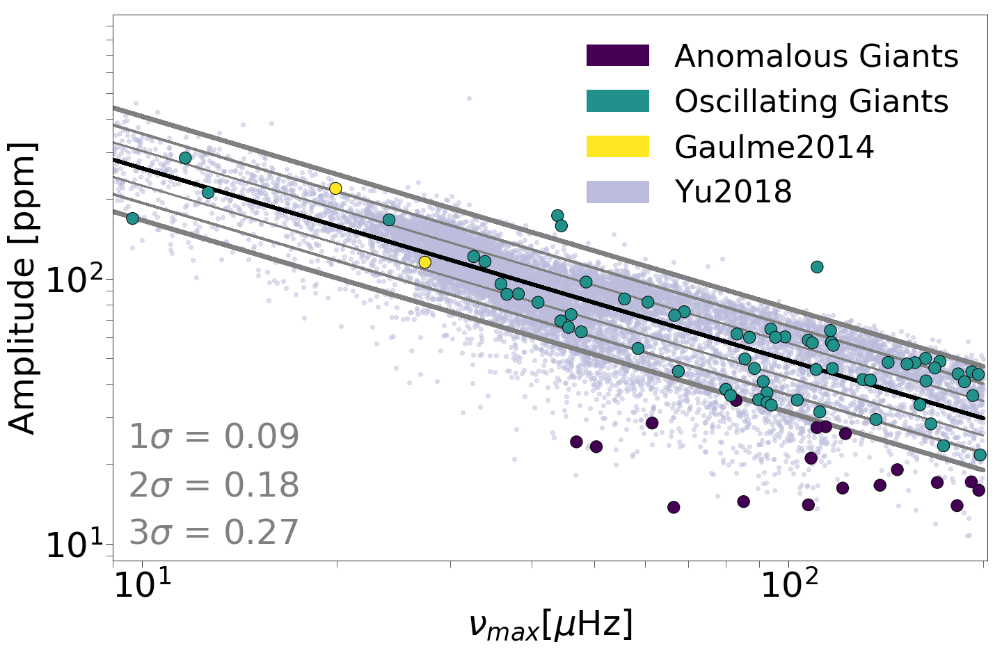
Figure 1: The amplitude of oscillations versus frequency of maximum power for the red giants in our sample (colored circles) and the red giants in Yu et al. (2018) (light blue dots). The black line shows a linear fit whilst the gray lines correspond to 1, 2 and 3$\sigma$ limits (each of these limits is quantified in the bottom left of the plot). Green circles are oscillating stars whilst purple circles are anomalous. Yellow stars are part of the G14 sample. This sample is restricted to the Yu et al. (2018) selection criteria and therefore does not include the entirety of our red giant sample or the Gaulme et al. (2014) sample.

Table 1: Robo-AO Sample Breakdown

	Dwarfs	Giants
Oscillating	100	99
Anomalous	54	55

This lack of oscillations could suggest a significant physical difference between stars sharing similar fundamental properties. Alternatively, inaccurate stellar properties could be used to mischaracterize a star as oscillating (Chaplin et al., 2011b). For example, the inferred oscillation amplitude of a star will be overestimated if the stellar type is based on an overestimated luminosity. In fact, the star may exhibit oscillation amplitudes which are too small to be observed by Kepler.

A lack of oscillations could also be attributed to multiplicity; either via the dilution of amplitudes caused by contaminating flux (Schonhut-Stasik et al., 2017), or by spectroscopic binaries, inhibiting oscillations through tidal interaction. Tidal interactions between stars are believed to increase magnetic activity and subsequently decreases the efficiency of the surface convection that drives oscillations, inducing amplitude suppression. Gaulme et al. (2014) (hereafter G14) demonstrated a link between amplitude suppression and close binaries using Kepler observations of 19 red giant eclipsing binary systems. Fifteen of the red giants demonstrated solar-like oscillations, whilst there were oscillations detected in the remaining four. The stars with no mode detections exhibit shorter orbital periods (between 15 and 45 days). For individual modes, the relationship between oscillations and binarity has also been investigated. For example, it has been found that detached eclipsing binaries present p-dominated mixed-modes more often (Themeßl et al., 2017).

It is plausible that systems can contain both a wide and spectroscopic companion, suggesting that multiple mechanisms can act simultaneously to suppress amplitudes. These systems can occur frequently. Tokovinin et al. (2006) found a 96% likelihood that a solar-type spectroscopic binary system (with an orbital period of $<$3 days) will also contain a tertiary companion.

Despite the discovery of these links between oscillations and multiplicity, there have been no large-scale statistical studies on the effects of multiplicity on oscillation formation and detection.

In this work we investigate the effect of multiplicity on stellar oscillations, through a large combined imaging and spectroscopic campaign. We identify wide companions which may cause amplitude dilution by observing 327 Kepler asteroseismic stars using Robo-AO. We search for spectroscopic companions to stars that may be causing tidal interference using ESPaDOnS at the Canada France Hawai’i Telescope (CFHT). ESPaDOnS performed multi-epoch, high-resolution spectroscopy for a sub-sample of 34 targets containing both single stars and wide binaries. Our imaging sample also contains the 19 red giant eclipsing binaries from G14. Imaging these stars will determine whether a wide companion is also present in their system, building on the findings of Tokovinin et al. (2006).

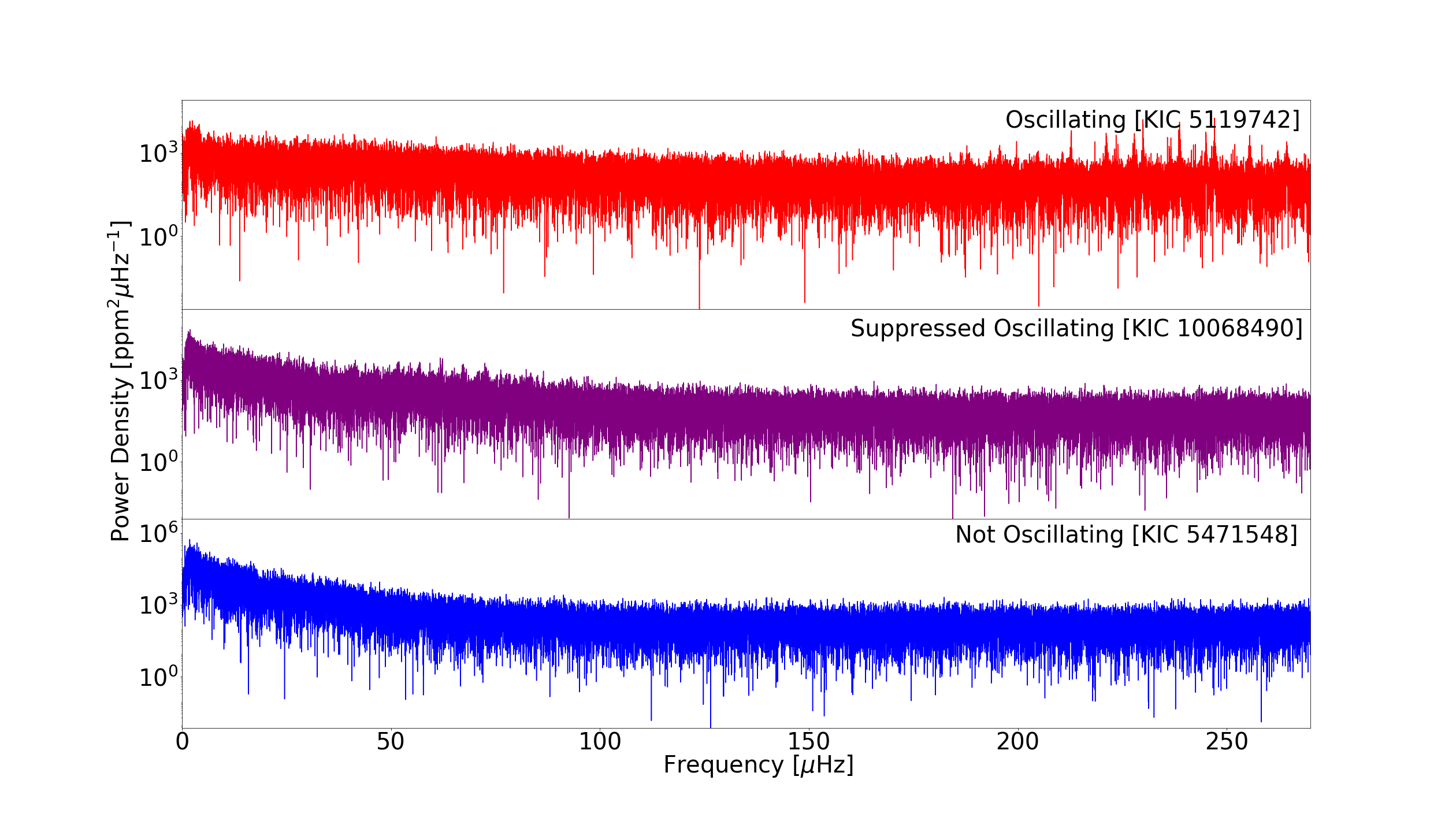
Figure 2: Three Kepler power spectra for an oscillating, suppressed and non-oscillating giant star. Top: KIC 5119742 with oscillations around 230$\mu$Hz. Middle: Suppressed oscillations in KIC 10068490; slight oscillations around 65$\mu$Hz. Bottom: No oscillations (KIC 5471548).

2 Target Selection

Our sample contains 327 dwarf (log(g) $>$3.5) and red giant (log(g) $<$3.5) stars predicted to display solar-like oscillations. Oscillating red giants, as well as oscillating and anomalous dwarfs were randomly selected from the APOKASC catalog. Anomalous red giants were identified via visual inspection of spectroscopically confirmed red giants in the APOKASC catalog (Pinsonneault et al., 2014). Table 1 organises the sample into sub-categories: dwarfs and giants; oscillating and anomalous.

We used stellar parameters to calculate the detection probability: the probability that oscillations would be detected above the Kepler detection limit as described in Chaplin et al. (2011c). Detection probability was calculated for all dwarfs using temperature values from the Kepler Stellar Properties Catalog (KSPC) (Mathur et al., 2017) and updated radii from Gaia Data Release 2 (DR2) (Gaia Collaboration et al., 2018; Berger et al., 2018). We then separated dwarfs into anomalous and oscillating groups, based on a limit of $\geq$90% detection probability for oscillations.

All giants have a detection probability of 100%, based on their large pulsation amplitudes. There is a well understood relation between amplitude and frequency of maximum power ($\nu_{max}$) (Huber et al., 2011), so if a star has a much lower amplitude value than expected, we can define it as anomalous. To categorize giants we used amplitude and $\nu_{max}$ values from Yu et al. (2018), which contains precise estimates of asteroseismic properties for 16,000 Kepler red giants, some of which overlap with our sample. Figure 1 shows the data from Yu et al. (2018) and a fit to the $\nu_{max}$-amplitude relation with 3$\sigma$ limits. We defined all stars 3$\sigma$ below the fit to be anomalous. Stars appearing 3$\sigma$ upward of the fit are likely high amplitude red giants, whose large amplitudes are thought to be due to triple systems, with a red giant and wide main-sequence binary contaminating the pixel aperture (Colman et al., 2017).

For stars in the Yu et al. (2018) data set with $\nu_{max}>200\mu Hz$, no amplitudes are listed. This is because at $\nu_{max}>200\mu Hz$ it becomes difficult to fit the power spectrum background. These targets were marked as oscillating. Stars not included in the Yu et al. (2018) work were grouped based on a visual inspection of oscillations in their power spectra. Figure 2 illustrates example power spectra for three giant stars showing oscillations, suppression of oscillations, and no oscillations respectively. One star had no available power spectra and was not present in Yu et al. (2018) so it was marked as oscillating as is expected for giants.

3 Observations and Data Reduction

3.1 Robo-AO

We used the Robo-AO robotic laser AO system (Baranec et al., 2014), mounted on the 2.1m telescope at Kitt Peak, Arizona (Jensen-Clem et al., 2018), to obtain high angular resolution images of our full target sample (327 stars). Robo-AO observations took place between 2016 June 07 and 2017 May 28, across 20 nights, with 140 objects observed more than once to ensure high quality images. We used a total exposure time of 120s that enabled the detection of additional sources up to $\sim$6 magnitudes fainter than the target. We took all observations in the i' filter (our stars range from magnitudes of 6.8 to 14 in i band). More information on the magnitude limits of observations at Kitt Peak can be found in Jensen-Clem et al. (2018).

We used the standard Robo-AO data reduction techniques described in Law et al. (2014). Table LABEL:short_long lists all Robo-AO observations, including Kepler Input Catalog (KIC) Identifier and i-band magnitudes. It also states whether a companion has been observed, either in this work or previously.

3.2 NIRC2

We used the NIRC2 infrared camera behind the Keck II AO system to confirm all the wide companion candidates, and obtain supplementary near-infrared photometry. We observed the targets on 2016 September 12, 13 and 2017 July 31. We operated NIRC2 in its 9.9 mas pixel^-1 mode which results in a field of view of $\sim$10$\farcs$0. We obtained 3-point dithered images for each star, with total exposure times ranging from 36s to 240s. We used the J, K’ and PK-continuum filters (central wavelengths 1.248$\mu$m, 2.124$\mu$m, 2.2706$\mu$m and , respectively) choosing a filter consistent with achieving the best image of both star and companion.

Each image from NIRC2 underwent sky subtraction and flat-field calibration. Flat-field frames were taken at the beginning of each night, and dark subtraction was performed with an unused quadrant of the detector. Each frame was corrected for bad pixels, and stacked to create a final image.

3.3 ESPaDOnS

ESPaDOnS is a high resolution echelle spectrograph at CFHT on Maunakea, Hawai’i. We chose a sub-sample of 34 stars, as observing constraints would not allow a multi-epoch survey of the entire target sample. The sub-sample contains both single stars (18) and stars with wide companions observed by Robo-AO in the imaging stage (15). We used ESPaDOnS to obtain at least three epochs of spectroscopy between 2017 and 2018, with the exception of KIC 893836, which was only observed twice but still included in analysis. Table 3 organises this sample into the same categories as Table 1. Observations had an average signal-to-noise ratio (SNR) of $\sim$80 per frequency resolution element, at an average resolution of R$\sim$80,000.

ESPaDOnS data is delivered to the user fully reduced using the Libre-ESpRIT reduction package (Donati et al., 1997). This package performs bias subtraction, flat-fielding, masking of bad pixels, wavelength calibration and spectrum extraction. The output provided contains several data analysis options: a continuum normalized spectrum, a corrected spectrum based on telluric lines or a combination of these options. We chose the continuum normalized data with the barycentric correction. Table LABEL:Spectra describes these observations as well as the results from the data analysis stage.

We included an eclipsing binary system from G14 in the spectroscopic sample: KIC 5308778. This star provided a test for whether our method was capable of revealing an RV scatter consistent with a spectroscopic binary.

4 Data Analysis

4.1 AO Companions

Table 2: Full Robo-AO Observation List

KIC ID	Mag	Obs	Companion?	Category
(KOI)	i’	Date
1430163	9.49	20160704		DO
1430239	10.39	20160704		DA
1571152	9.24	20160704	Both	DA
1576249	11.33	20160607	Wide	DA
1725815	10.71	20160607	Both	DO
1870433	12.34	20160704		GA
2140561	12.50	20160704		GA
2285032	11.25	20160704		GA
…	…	…	…	…

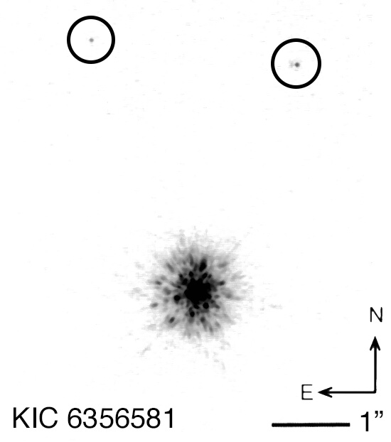
Figure 3: Reduced NIRC2 image of triple system KIC 6356581. This image has been adjusted for contrast using SAO DS9, allowing the secondary and tertiary to be visible; both are circled. Neither of these companion stars is found to be physically associated i.e. they do not appear to be at a similar distance to the primary star.

4.1.1 Companion Detection and System Confirmation

All detected wide candidate companion systems needed to be visually resolved in the full frame or PSF-subtracted image, in order to deduce system parameters using aperture photometry or PSF-fitting. To identify companions in the Robo-AO data we visually inspected the images for secondary stars with separations $\leq$4$\farcs$0, the size of a Kepler pixel. Contaminating secondary stars may exist inside the [larger] Kepler aperture, but these would be detectable in seeing-limited surveys and are therefore not included here. The search was aided by the Robo-AO data visualization and characterization GUI (Lamman et al. (in prep.)).

Table 3: ESPaDOnS Sample Breakdown

	Dwarfs	Giants
Oscillating	18	5
Anomalous	7	3

We then confirmed our detections using an automated companion detection algorithm developed for the Robo-AO Kepler Object of Interest (KOI) surveys (see Ziegler et al. 2016). A detection significance was found for each candidate companion by sampling and modeling the background noise level as a function of radial distance from the target star. We then slid an aperture of the diffraction-limited FWHM diameter along concentric annuli centered on the target star. Possible astrophysical detections are identified when the enclosed flux of the aperture becomes significantly greater than the local noise. In this sample of brighter stars, bright speckles can produce high-significance detections, which we discarded. We chose the significance value for which the companion pixel coordinates we manual identified matched with the pixel coordinates of the significance detection method.

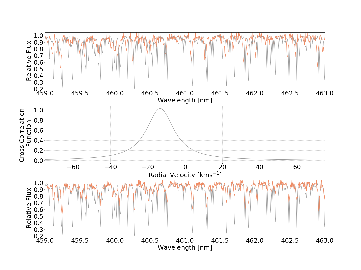
Figure 4: ESPaDOnS spectra of a target, KIC 10124866, (orange) and standard star (gray). Top: Original spectra. Middle: Cross-correlation used to determine the radial velocity. Bottom: Shifted spectra once the cross-correlation has been applied.

All companions visually detected in the full frame images can be seen in Figure A of the Appendix, whilst stars identified in the PSF-subtracted images can be seen in Figure B of the Appendix. All detected companions from Robo-AO images were observationally confirmed using NIRC2. For three of these systems the NIRC2 observations revealed additional tertiary stars that remained undetected by Robo-AO, an example of which can be seen in Figure 3.

We used these identified systems to calculate a companion fraction for anomalous and oscillating stars. A companion fraction is defined as the percentage of stars that have at least one discovered companion. This companion could be a wide companion (either physically associated or coincident) or a spectroscopic companion. When quoting companion fractions we used one of two uncertainties. Poisson errors apply only in the case of large samples so for N$>$100, errors are calculated in this way. For N$<$100 binomial errors were used. This latter method is taken from Burgasser et al. (2003) where statistical uncertainties are derived by constructing a probability distribution for the total sample size, N, and the number of binaries in the sample, n. The binomial distribution determines the probability of finding n binaries given the sample size and binary fraction.

4.1.2 Separation and Position Angle

We calculated separation and position angle between the primary and secondary stars with the same technique as Schonhut-Stasik et al. (2017), adapted for Robo-AO at Kitt Peak. We tested this method with Palomar data from Baranec et al. (2016) and Kitt Peak data from Ziegler et al. (2018a) reproducing separation, position angle and uncertainty values. For pairs too close to resolve in the reduced image, coordinates from a PSF-subtracted image were used by shifting them to the frame of the reduced image.

Pixel coordinates were determined using the Aperture Photometry Tool (APT) (Laher et al., 2012), except for KIC 3430893 where APT could not lock on correctly to either the full frame or PSF-subtracted image. In this case, coordinates were determined using SAO DS9, by taking an average of manual measurements of the central pixel for the star in question. We also manually determined the separation for tertiary companions identified in NIRC2, with the error equivalent to the size of a NIRC2 pixel, i.e. 0$\farcs$01.

4.1.3 Contrast Ratios and Amplitude Dilution

Flux ratios were calculated using PSF-photometry, designed using the Astropy module Photutils. We calculated the ratio by using Gaussian models to fit the centroid coordinates of each star, determining their relative flux ratio.

For magnitude differences, as well as individual magnitudes and fluxes, we used the method from Schonhut-Stasik et al. (2017) for both Robo-AO and NIRC2 data. To find individual magnitudes we compared the flux ratio to the total magnitude of the system, taken from the KIC. We used i-band for the total system magnitudes of the Robo-AO images and different bands for the NIRC2 images depending on the filter, (K for K’ and PK-continuum, J for J). We note that i-band corrections may be overestimated for widely separated sources, given the typical $\sim$2$\farcs$5 resolution of KIC photometry (Brown et al., 2011).

Amplitude dilution is defined as the percentage of flux observed from the system that is a result of the secondary star:

$$A=\frac{F_{2}}{F_{1}+F_{2}}\times 100$$ (1)

with $F_{1}$ and $F_{2}$ corresponding to primary and secondary fluxes, respectively. The effect of amplitude dilution is larger in triple systems containing two wide companions. When only one companion accompanies the primary star, the companion can only dilute the flux by a maximum of 50%. However, in a three star system, with two extra stars, the maximum amplitude dilution is 67%, with each star contributing a third of the flux.

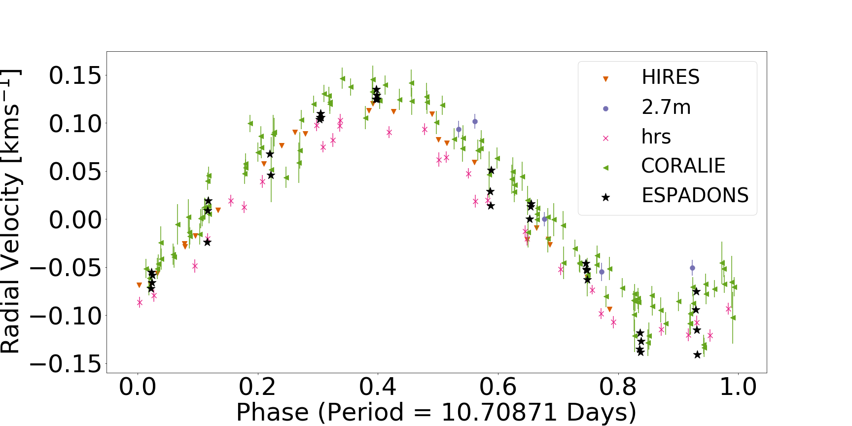
Figure 5: Reproduction of the planet phase curve from Hinkel et al. (2015) demonstrating that HIP72339 hosts a hot Jupiter. Each marker and color represents a different set of observations from a different telescope. Radial velocities determined in this work (using data from Fares et al. (2013)) are marked by black stars.

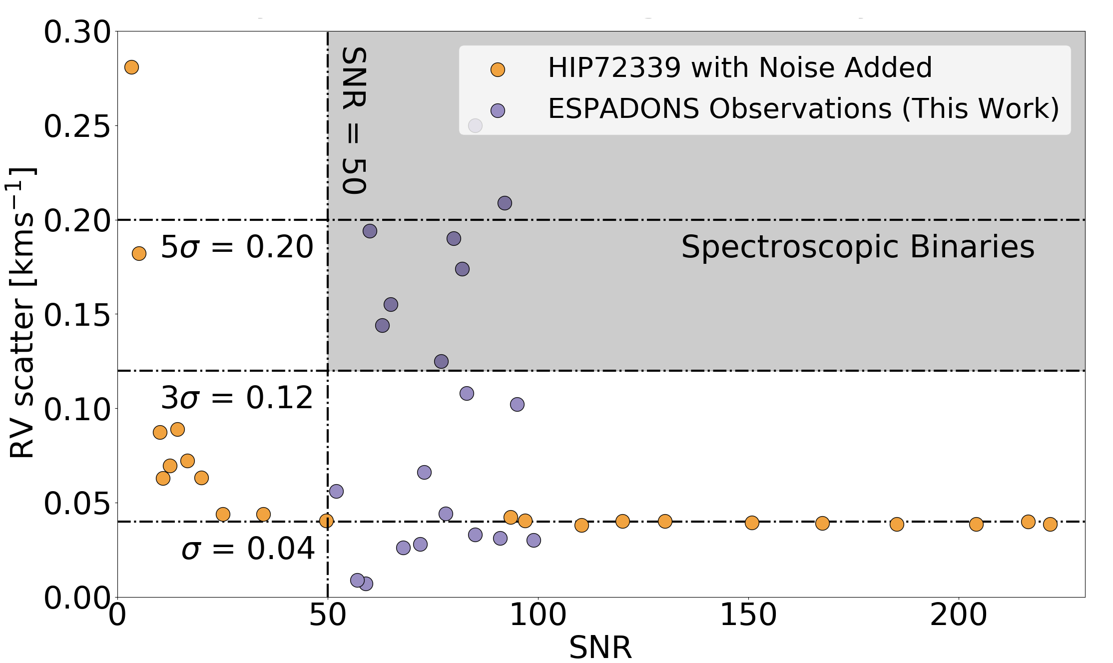
Figure 6: Radial velocity scatter versus SNR. Orange symbols represent the standard star with a varying SNR, simulated by adding Gaussian noise to the spectra. Purple symbols illustrate our target sample. The horizontal dashed line marks the 1$\sigma$ limit. Above 3$\sigma$ we define our targets to be RV variable due to a stellar companion (shaded area). The y-axis has been truncated to not include the larger values of RV scatter.

4.1.4 Companion Characterization

Primary spectral types were taken from the SIMBAD database (Wenger et al., 2000), or if unavailable, were inferred from the effective temperature of the primary star using Table 5 in Kraus & Hillenbrand (2007). This assumes that the companion had a negligible effect. Parameters for the wide systems can be found in Table LABEL:CompDet. Statistical analysis of those systems is presented in Section 5.

Where available, we used Gaia DR2 for updated radii (Berger et al., 2018) and distance measurements for both stars. We used primary target RA and Dec from SIMBAD or KSPC and a 5$\farcs$0 circluar aperture, to search for detected companions in the DR2 database. Separation was calculated using RA and Dec values for any other stars located in the aperture, to confirm whether the companion identified with Robo-AO was also identified with Gaia. Nine primary targets had no Gaia radius so KSPC values were used.

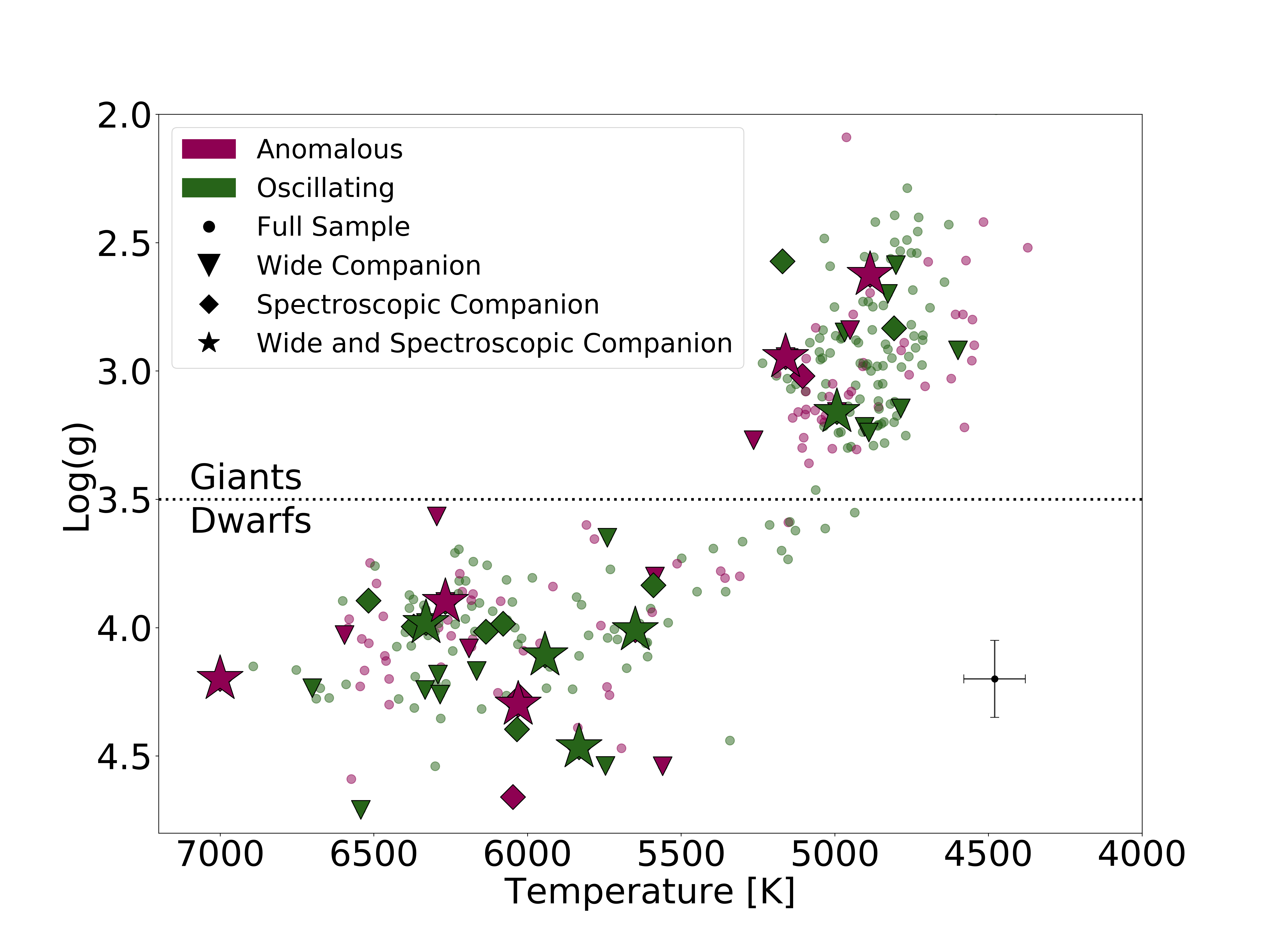
Figure 7: H-R diagram showing the full sample of oscillating (green) and anomalous (purple) stars with surface gravity on the y-axis and temperature on the x-axis (both from KSPC). The error shown (100K for temperature and 0.15 dex for surface gravity) is a typical uncertainty for the whole sample. A line separates the dwarfs and giants at log(g) = 3.5. The circles in this plot represent the targets for which no companions were found. Targets with a wide companion are shown by a downward facing triangle, the spectroscopic binaries are marked by a diamond and targets with both a wide and spectroscopic companion are marked by a star.

4.1.5 Physical Association

Physical association between the two stars in a system was determined by calculating whether their distances agree within their uncertainties to 1$\sigma$. If the distance to a star was not available in Gaia, but we had a K’ or PK-continuum band NIRC2 observation, we used the method described in Atkinson et al. (2017) (hereafter A17). This method uses broadband photometry to determine radii, spectral types and distances to stars. If possible, we used both A17 and Gaia to compare computed distances and determine the accuracy of the A17 model. If the distances given by A17 and Gaia agreed within uncertainty, we adopted the spectral type and radii for the secondary given by A17. The A17 model does not discriminate between dwarfs and giants and in these cases will give an incorrect distance, therefore these radii and spectral type were not included. These values can be found in Table LABEL:CompDet3.

Both Ziegler et al. (2018b) and Hirsch et al. (2017) found that most binary systems with separations of $\leq$1$\farcs$0 are physically associated. We adopt this for all our binaries at $\leq$1$\farcs$0 without derived distances (unavailable in Gaia and no appropriate NIRC2 images).

4.2 Spectroscopic Companions

4.2.1 Radial Velocities

We used spectroscopy to identify binaries too close to be resolved using AO imaging. We detected companion systems by measuring the scatter in radial velocity (RV) of a star over at least three epochs.

To determine the RV of each observation we used a cross-correlation function (as implemented in pyasl with a step size of 0.001kms^-1) to compare to a standard star, as demonstrated in Figure 4. We found the absolute RV values by subtracting the RV of the standard (in this case -11.85kms^-1). The RV value for an observation was found from the peak of the cross-correlation curve. We took the RV scatter as the standard deviation of all the RV values for a star.

For wavelength ranges, we chose 459nm - 463nm for cooler stars and 490nm - 495nm for hotter stars, containing as many lines as possible without including strong telluric lines. We were careful to include a similar number of lines in both hot and cold stellar spectra, so we could assume a standard RV uncertainty amongst all stars.

4.2.2 The Standard Star

To choose a standard, we tested stars from Soubiran et al. (2013) who created a catalog of 1420 RV standards to calibrate spectroscopic measurements for Gaia. Our standard star needed multiple ESPaDOnS observations (taken from the Canada Astronomy Data Centre) and a high SNR.

The best candidate to meet these criteria was HIP72339, which incidentally hosts a hot Jupiter first discovered in Udry et al. (2000). We used the presence of a planet to test the accuracy of our cross-correlation function, by reproducing the phase curve of the planet from Hinkel et al. (2015) (see Figure 5). Our ability to identify this hot Jupiter is evidence that our method is adequate for discovering spectroscopic binaries.

As HIP72339 is not in the Kepler field, we also ran a number of cross-correlations using Kepler stars from our sample, in order to ensure that error would not be introduced using this standard.

4.2.3 RV Uncertainties

To determine which values of RV scatter should be considered indicative of a spectroscopic binary, we calculated a lower limit for the RV scatter, by building a relationship between RV scatter and SNR.

The average SNR for the HIP72339 observations was higher than our targets, allowing us to use the standard to dictate a lower limit. We plotted the SNR versus RV scatter (with the planet subtracted out) for observations of HIP72339 with various quality levels. We varied the quality level by adding random noise from a Gaussian distribution. We obtained the SNR from the continuum of the spectra, by measuring the mean of the points around 606nm, where there are no spectral lines. We obtained the standard scatter by cross-correlating against another observation of the standard and plotted the RV scatter as a function of SNR for each iteration of the observation + noise. The result of this can be seen in Figure 6.

We then calculated a SNR for each set of target observations and overplotted these on to the values of HIP72339. The values of SNR versus scatter for HIP72339 stayed consistent down to $\sim$30. As all our target observations had an SNR$>$50, we chose $\sigma$=0.04kms^-1 to be our lower limit. This corresponds to the mean of the HIP72339 observations with SNR$>$30. This value gave us a 3$\sigma$ detection of 0.12kms^-1 and a 5$\sigma$ detection of 0.20kms^-1.

5 Results

5.1 All Companions

All the systems identified in this survey are summarized in Figure 7, which shows no trend in where the stars lie on the H-R diagram.

We compared the overall companion fraction of oscillating and anomalous stars (Figure 8(a)) and found that they agree within uncertainty, suggesting no difference in multiplicity between the groups. This companion fraction includes any system with at least one wide or spectroscopic companion; systems with multiple companions are only considered once.

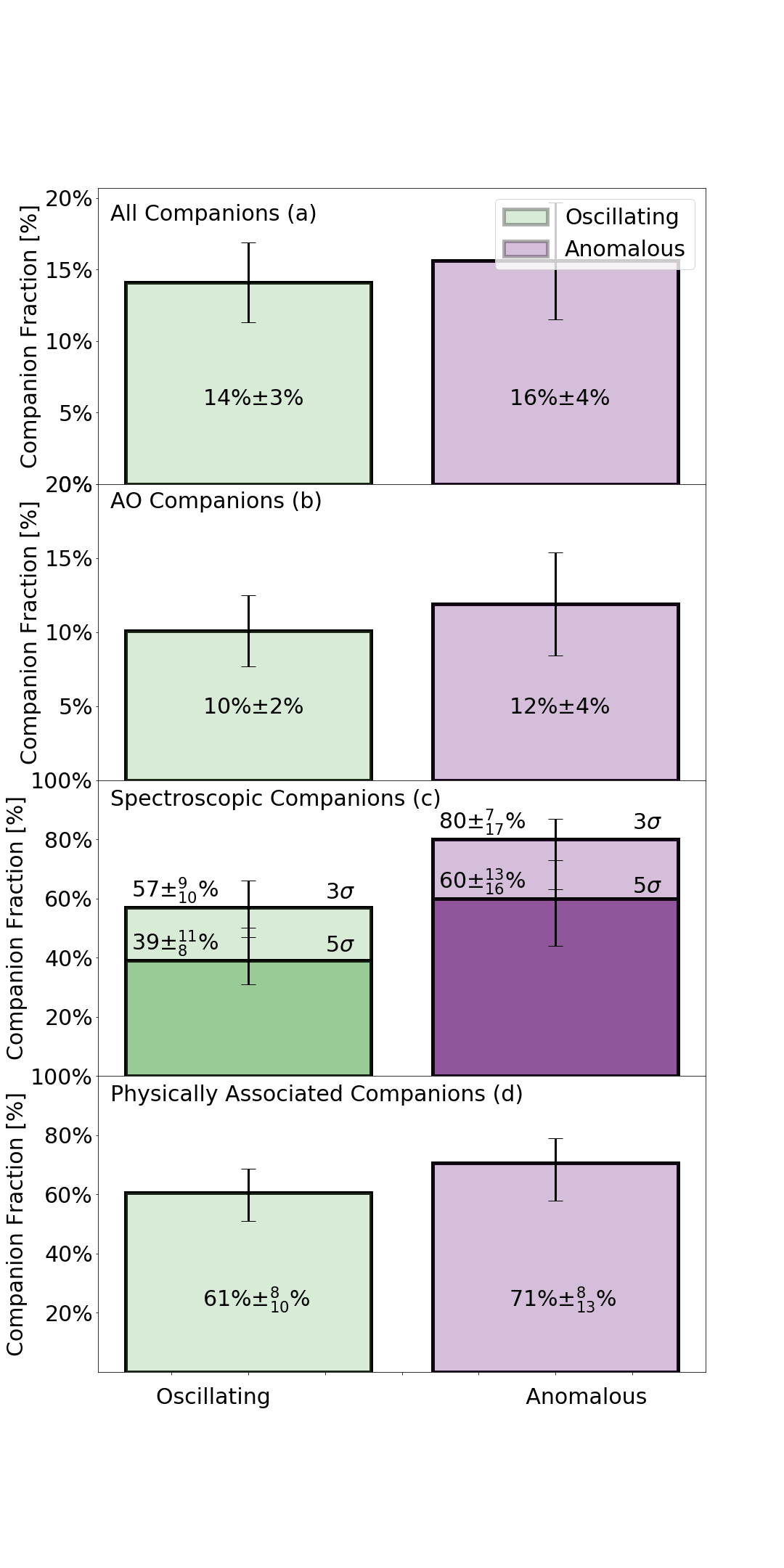
Figure 8: Companion fractions for oscillating (green) and anomalous (purple) systems. Top: All companion systems. Second from Top: AO/wide companions. Third from Top: Spectroscopic companions and Bottom: Physically associated companions. Uncertainties are calculated using binomial or Poisson statistics depending on the sample size.

Table 4: Radial Velocity Shifts for Spectroscopic Data

KIC ID	Julian	Radial	Sigma	Standard	Signal to
	Date	Velocity	Likelihood	Deviation	Noise Ratio
	[Modified]	[kms-1]		[kms-1]
1571152	57884.468353	7.150	5	2.131	93 [86]
	58005.2196723	9.437			92
	58297.6207027	7.149			113
	58360.4760237	9.187			61
	58391.3431338	3.487			88
1725815	57884.5152016	24.778	5	2.433	84 [87]
	57972.385056	23.241			81
	58321.3778602	19.024			96
3115178	57879.564732	-26.694	1	0.056	60 [52]
	57979.3868736	-26.674			42
	58298.580257	-26.567			61
…	…	…	…	…	…

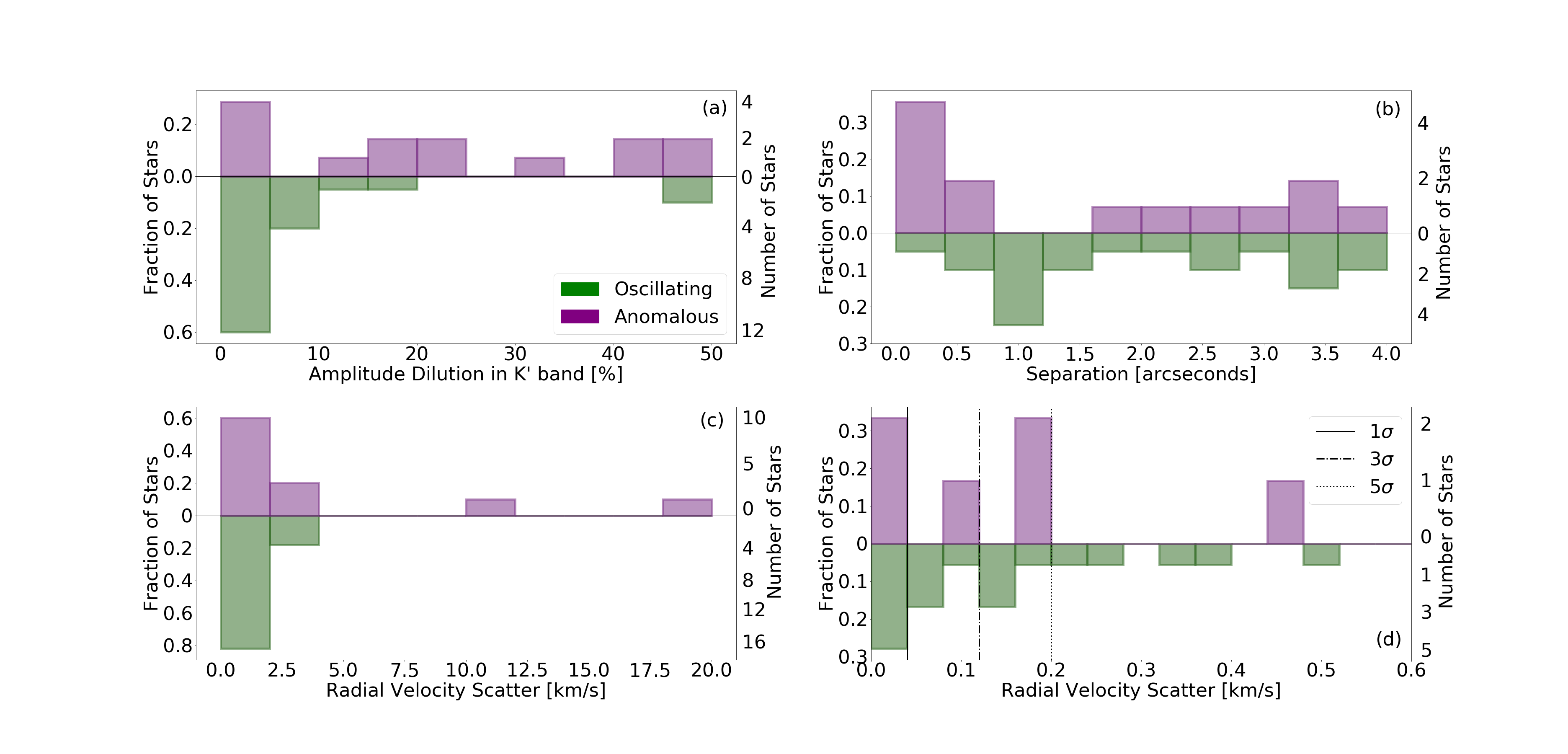
Figure 9: Plots showing the distribution of companion systems in the oscillating and anomalous groups as a function of system parameters. Top Left: Distribution as a function of amplitude dilution in the K’-band (%). Top Right: Distribution as a function of separation from the primary star (arcseconds). Bottom Left: Distribution as a function of the radial velocity scatter (kms^-1). Bottom Right: Distribution as a function of radial velocity scatter up to 0.6kms^-1 (kms^-1). Also showing 1, 3 and 5$\sigma$ lines.

5.2 AO/Wide Companions

We identified 34 systems with at least one wide companion (11%$\pm$2% companion fraction) and 18 systems containing a companion which may be physically associated (6%$\pm$1% companion fraction). We find four systems with more than one wide companion, however none with more than one physically associated wide companion. These statistics do not include the G14 sample.

The system with smallest separation is KIC 2568519 at 0$\farcs$16 $\pm$ 0$\farcs$08, almost at the diffraction limit of Robo-AO. Three triple systems were observed: KIC 3221671, KIC 6356581 and KIC 8983847. KIC 5123145 is a quadruple system.

5.3 Spectroscopic Companions

We found 15 spectroscopic binaries, giving a companion fraction of 41$\%^{+11\%}_{-9\%}$ when considering a 5$\sigma$ lower limit. The highest RV scatter was 19.745kms^-1 for KIC 5308778, a known G14 binary. The second largest was KIC 11551430 with an RV scatter of 19.0kms^-1. Five systems were found to have both a wide and spectroscopic companion (to 5$\sigma$) and four where both components are physically associated.

5.4 Comparison to Other Surveys

The companion fraction for the oscillating dwarf group (18%$\pm$5%) is lower than the value from Raghavan et al. (2010), who find a companion fraction of $\sim$45% for FGK dwarfs. Our lower fraction is likely due to the fact our survey truncates possible binaries at 4$\farcs$, whereas some methods in Raghavan et al. (2010) identify binaries out to 200$\farcs$. We were unable to compare our anomalous systems to Raghavan et al. (2010) as they were chosen for possible binarity and therefore present a selection bias.

To compare our companion fraction with a similar sample also observed with Robo-AO, we used values from their KOI survey (Ziegler et al., 2018a). We combined the oscillating dwarfs in our work with a sample of 99 oscillating Kepler dwarfs and subgiants from Schonhut-Stasik et al. (2017) to produce a companion fraction representing dwarf and subgiant solar-like oscillators. Excluding giants makes the asteroseismic sample more consistent with the KOI sample. We found the companion fraction of the KOI survey (14.5% $\pm$ 0.5%) to be in agreement with ours (13% $\pm$ 3%).

We were unable to compare the dwarf and giant samples to one another due to the bias in completeness for the oscillations and for the binary detection. For the remainder of this analysis the oscillating and anomalous groups contain both dwarfs and giants. This should not effect overall binary fraction as there are roughly the same number of dwarfs and giants in each category.

6 Discussion

6.1 Wide Companions

Figure 8(b) compares the companion fraction of wide binaries in the oscillating and anomalous groups, showing that anomalous stars are no more likely to have a wide companion than oscillating stars. This calculation considers each system only once, regardless of the number of companion stars within it.

Figure 9(a) shows the distribution of wide companions as a function of their amplitude dilution in K’-band. For amplitude dilutions $>$10%, more systems belong to the anomalous group. This suggests there may be a lower limit to the amount of amplitude dilution necessary, in order to reduce observed oscillations below the Kepler detection limit.

Figure 9(b) shows the distribution of wide companions as a function of their separation from the primary star. It shows more companions to anomalous stars at close separations of $\leq$1$\farcs$. Closer companions are more likely to be physically associated equal mass companions (Raghavan et al., 2010) than companions at a wider separation. This suggests a higher value of amplitude dilution for closely separated systems, as the secondary star will be contributing a greater flux. In Figure 10 we have shown that at $>$2$\farcs$0 separation, generally all amplitude dilutions are $<$10%. This reiterates that larger values of amplitude dilution are more likely at close separations.

6.2 Spectroscopic Companions

Figure 8(c) compares the companion fractions for the spectroscopic sample between the oscillating and anomalous groups. The companion fractions agree for both the 3$\sigma$ and 5$\sigma$ limit.

Figure 9(c) and (d) demonstrate the distribution in radial velocity scatter for the spectroscopic companions found in both the oscillating and anomalous samples. We tentatively observe higher RV scatter in the anomalous stars.

As this work contains a large number of both oscillating and anomalous stars, we can assume that the companion mass and inclination distribution are the same for both groups. Therefore, we can interpret this finding as demonstrating a higher fraction of close companions in anomalous stars.

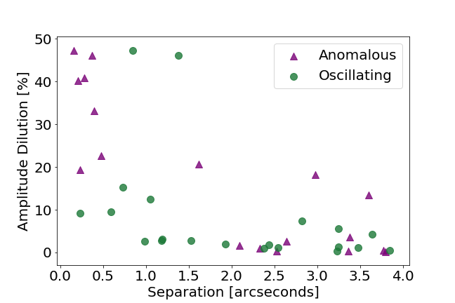
Figure 10: Amplitude dilution (in K’ band) as a function of separation (arcseconds) for both the oscillating and anomalous wide companion systems. Purple triangles represent anomalous wide companion systems and green circles represent oscillating wide companion system.

6.3 Triple Systems With Both a Wide and Spectroscopic Companion

We observed both the G14 sample with direct imaging and a sub-sample of the wide binaries with spectroscopy. This allowed us to further investigate the results of Tokovinin et al. (2006), who found that the presence of a spectroscopic binary is indicative of a wide companion.

We did not find any wide companions to the G14 stars. This could be explained if our sensitivity did not achieve the necessary contrast ratio. Alternatively, Tokovinin et al. (2006) states that the probability of a wide tertiary companion drops from 96% to 34% with an orbital period increase from 3 to 12 days. The minimum period in the G14 sample is $\sim$15 days, therefore the lack of wide companions could indicate the probability of a wide tertiary companion continues to decrease with increased orbital period.

We found that $\sim$50% of the 3$\sigma$ spectroscopic binaries have a physically associated tertiary (as opposed to a possible coincident wide companion or no tertiary companion at all). This rate is in agreement with the value for stars without a spectroscopic binary but with a physically associated wide companion. Therefore, it is no more likely that we would find spectroscopic binaries in wide systems.

7 Conclusions

We observed 327 asteroseismic Kepler stars with AO imaging and 34 with spectroscopy, to investigate whether stellar multiplicity is related to the suppression of solar-like oscillations. Our main conclusions are as follows:

• We do not see a significant difference in companion fraction for wide companions between oscillating and anomalous stars (10% $\pm$ 2% and 12% $\pm$ 4% respectively; see Figure 8(b)). However, companions at separations of $<$0$\farcs$5, and demonstrating an amplitude dilution $>$10% are all anomalous. This suggests that the presence of a wide companion is not enough to assume a star will have suppressed oscillations and it could indicate a threshold below which the presence of excess flux will not reduce the amplitude enough to create a non-detection, although it may still contribute along with other factors (i.e. triple systems).

• We find tentative evidence for a higher fraction of spectroscopic binaries between anomalous and oscillating stars ($60\%\pm 3\%$ and $39\%^{+11\%}_{-8\%}$ respectively (5$\sigma$); see Figure 9(c)), as inferred from the radial velocity scatter measured over multiple epochs. This would be in line with the suggestion by Gaulme et al. (2014) that tidal interactions in close eclipsing binary systems may suppress the convective driving of solar-like oscillations. Further observations of a larger number of systems with an extended baseline of spectroscopic follow-up will be required to confirm this result.

• Although companion systems are a likely mechanism for the non-detection on oscillations in some stars, it is probably not the only mechanism. There are still 75 anomalous stars in this sample (109 total) for which no companion has been detected. This does not rule out multiplicity as it is likely that not all companions were discovered in this work. This could be due to separations too close for AO imaging to resolve but too far out for spectroscopy. It could also mean their oscillation suppression comes from another source, such as increased levels of stellar activity. A study of stellar activity in our sample is beyond the scope of this paper.

• For all physically associated wide companion systems that were also surveyed with ESPaDOnS, $\sim$50% contain a spectroscopic binary to 3$\sigma$, consistent with the spectroscopic companion fraction for single systems. We did not find any wide companions to the G14 sample. This may be because the probability of a wide tertiary companion decreases with the increased orbital period of the close binary Tokovinin et al. (2006). In the G14 sample all the eclipsing binaries have orbital periods $\geq$15 days, larger than those in the Tokovinin et al. (2006) sample.

The Transiting Exoplanet Survey Satellite (TESS) mission is observing an order of magnitude more asteroseismic stars than Kepler. TESS has 21$\farcs$ pixels, so determining multiplicity will be even more crucial as more blended binaries in the aperture can add flux to the primary light curve. Robo-AO will be used to vet the majority of TESS candidate exoplanet host stars (Ziegler et al., 2018), and in a similar process, can also be used to find candidate stellar companions to asteroseismic stars. Thorough and timely follow-up will be required to reassess amplitude dilution in this much larger sample of asteroseismic targets.

Table 5: Detected Companion Systems

KIC ID	Separation	Position	Magnitude	Magnitude	i' Detection	System	Amplitude	Amplitude
	(″)	Angle	Difference	Difference	Significance	Spectral	Dilution	Dilution
		(∘)	i'	K’	($\sigma$)	Type	i' (%)	K’ (%)
1571152	0.40 $\pm$ 0.06	126 $\pm$ 2	0.91 $\pm$ 0.11	0.76 $\pm$ 0.18	7.99	F2V	30.20 $\pm$ 0.40	33.24 $\pm$ 9.16
1576249	0.28 $\pm$ 0.06	164 $\pm$ 7	0.62 $\pm$ 0.21	0.40 $\pm$ 1.90	5.66	F7V	36.20 $\pm$ 0.45	40.94 $\pm$ 136.44
1725815	3.64 $\pm$ 0.06	81 $\pm$ 2	3.81 $\pm$ 0.20	3.22 $\pm$ 0.17	8.67	F7V	2.91 $\pm$ 0.05	4.19 $\pm$ 1.31
2568519	0.16 $\pm$ 0.08	74 $\pm$ 12	0.94 $\pm$ 0.22	0.29 $\pm$ 0.20	8.42	F7V	27.70 $\pm$ 3.99	47.35 $\pm$ 15.57
3123191	0.73 $\pm$ 0.06	122 $\pm$ 3	1.91 $\pm$ 0.21	1.86 $\pm$ 0.16	5.24	F7V	14.47 $\pm$ 0.24	15.26 $\pm$ 3.78
3221671(1)	1.62 $\pm$ 0.06	217 $\pm$ 2	2.56 $\pm$ 0.20	1.46 $\pm$ 0.17	7.73	F5V	8.66 $\pm$ 0.15	20.63 $\pm$ 5.3
3221671(2)	2.09 $\pm$ 0.01	…	…	4.43 $\pm$ 0.17	…	…	…	1.66 $\pm$ 0.42
3430893	1.18 $\pm$ 0.06	215 $\pm$ 2	3.37 $\pm$ 0.21	3.88 $\pm$ 0.16	$<$3	F7V	4.31 $\pm$ 0.08	2.73 $\pm$ 0.69
3643774	2.38 $\pm$ 0.06	106 $\pm$ 2	5.05 $\pm$ 0.19	5.04 $\pm$ 0.17	7.98	G1V	0.87 $\pm$ 0.02	0.96 $\pm$ 0.25
4260884	0.48 $\pm$ 0.06	177 $\pm$ 4	1.06 $\pm$ 0.21	1.33 $\pm$ 0.17	5.14	K3III	27.30 $\pm$ 0.38	22.72 $\pm$ 5.89
4914234	3.85 $\pm$ 0.06	165.8 $\pm$ 1.6	6.27 $\pm$ 0.22	5.81 $\pm$ 0.16	7.21	K3III	0.31 $\pm$ 0.01	0.47 $\pm$ 0.11
4999260	0.99 $\pm$ 0.06	342 $\pm$ 2	2.33 $\pm$ 0.21	3.96 $\pm$ 0.16	4.09	K3III	10.50 $\pm$ 0.18	2.55 $\pm$ 0.63
5123145(1)	2.64 $\pm$ 0.06	230 $\pm$ 2	4.03 $\pm$ 0.20	3.91 $\pm$ 0.17	5.52	K3III	2.38 $\pm$ 0.04	2.65 $\pm$ 0.70
5123145(2)	0.23$\pm$ 0.01	…	…	1.57 $\pm$ 0.17	…	…	…	19.43 $\pm$ 5.29
5123145(3)	3.77$\pm$ 0.01	…	…	5.91 $\pm$ 0.17	…	…	…	0.43 $\pm$ 0.12
5129882	2.33 $\pm$ 0.06	48 $\pm$ 2	5.24 $\pm$ 0.20	4.93 $\pm$ 0.17	10.14	K3III	0.79 $\pm$ 0.01	1.05 $\pm$ 0.27
5717541	1.19 $\pm$ 0.06	258 $\pm$ 2	3.44 $\pm$ 0.20	3.76 $\pm$ 0.17	8.71	K3III	4.05 $\pm$ 0.07	3.05 $\pm$ 0.84
5986270	2.82 $\pm$ 0.06	216 $\pm$ 2	3.27 $\pm$ 0.19	2.74 $\pm$ 0.17	10.37	K3III	4.70 $\pm$ 0.08	7.42 $\pm$ 1.94
6233558	3.38 $\pm$ 0.06	43 $\pm$ 2	3.97 $\pm$ 0.19	3.58 $\pm$ 0.17	15.43	K6III	2.53 $\pm$ 0.004	3.57 $\pm$ 0.96
6356581(1)	3.36 $\pm$ 0.06	337 $\pm$ 2	6.10 $\pm$ 0.19	6.29 $\pm$ 0.19	27.38	K3III	0.36 $\pm$ 0.01	0.30 $\pm$ 0.09
6356581(2)	3.80$\pm$ 0.01	…	…	6.80 $\pm$ 0.18	…	…	…	0.19 $\pm$ 0.06
6863041	0.59 $\pm$ 0.06	132 $\pm$ 3	2.40 $\pm$ 0.20	2.45 $\pm$ 0.17	7.86	G6V	9.92 $\pm$ 0.16	9.50 $\pm$ 2.50
7529180	2.44 $\pm$ 0.06	253 $\pm$ 2	6.52 $\pm$ 0.19	4.39 $\pm$ 0.16	7.17	F4V	0.25 $\pm$ 0.004	1.72 $\pm$ 0.43
7630743	3.48 $\pm$ 0.06	90 $\pm$ 2	4.80 $\pm$ 0.20	4.86 $\pm$ 0.17	6.31	K4III	1.19 $\pm$ 0.02	1.12 $\pm$ 0.29
7690843	0.23 $\pm$ 0.06	6 $\pm$ 8	0.81 $\pm$ 0.21	2.51 $\pm$ 0.17	$<$3	K3III	32.05 $\pm$ 0.43	9.19 $\pm$ 2.34
7801848	0.37 $\pm$ 0.06	325 $\pm$ 5	0.36 $\pm$ 0.22	0.17 $\pm$ 0.18	5.27	G3V	41.74 $\pm$ 0.49	46.10 $\pm$ 12.48
7901207	2.53 $\pm$ 0.06	201 $\pm$ 2	5.82 $\pm$ 0.19	6.05 $\pm$ 0.17	35.35	K3III	0.47 $\pm$ 0.01	0.38 $\pm$ 0.10
8542853	0.85 $\pm$ 0.06	297 $\pm$ 3	0.34 $\pm$ 0.21	0.120 $\pm$ 0.18	5.60	G7V	42.13 $\pm$ 0.48	47.37 $\pm$ 12.54
8983847(1)	2.54 $\pm$ 0.06	296 $\pm$ 2	4.90 $\pm$ 0.20	4.82 $\pm$ 0.17	7.29	K3III	1.08 $\pm$ 0.02	1.17 $\pm$ 0.30
8983847(2)	3.23 $\pm$ 0.06	238 $\pm$ 2	6.11 $\pm$ 0.26	6.47 $\pm$ 0.17	…	…	0.36 $\pm$ 0.01	0.26 $\pm$ 0.07
9702369	3.25 $\pm$ 0.06	353 $\pm$ 2	6.59 $\pm$ 0.19	4.72 $\pm$ 0.16	7.83	F7V	0.23 $\pm$ 0.004	1.27 $\pm$ 0.31
9965715	1.05 $\pm$ 0.06	152 $\pm$ 2	2.88 $\pm$ 0.21	2.11 $\pm$ 0.18	6.69	F7V	6.57 $\pm$ 0.12	12.55 $\pm$ 3.47
10124866	1.38 $\pm$ 0.06	186 $\pm$ 2	0.19 $\pm$ 0.21	0.17 $\pm$ 0.20	6.07	G2V	45.58 $\pm$ 0.49	46.12 $\pm$ 14.26
10140513	0.21 $\pm$ 0.06	76 $\pm$ 9	0.45 $\pm$ 0.22	0.43 $\pm$ 0.16	$<$3	F9V	39.78 $\pm$ 0.48	40.24 $\pm$ 9.57
10779537	1.93 $\pm$ 0.06	350 $\pm$ 2	4.54 $\pm$ 0.19	4.29 $\pm$ 0.17	10.23	K3III	1.50 $\pm$ 0.026	1.88 $\pm$ 0.50
10797849	2.98 $\pm$ 0.06	271 $\pm$ 2	1.78 $\pm$ 0.20	1.63 $\pm$ 0.15	5.73	F7V	16.27 $\pm$ 0.25	18.24 $\pm$ 4.13
10909629	1.53 $\pm$ 0.06	59 $\pm$ 2	4.24 $\pm$ 0.20	3.88 $\pm$ 0.16	10.41	F7V	1.98 $\pm$ 0.04	2.74 $\pm$ 0.68
11395018	3.25 $\pm$ 0.06	358 $\pm$ 2	2.95 $\pm$ 0.19	3.08 $\pm$ 0.17	8.21	G3V	6.17 $\pm$ 0.10	5.54 $\pm$ 1.43
11551430	3.60 $\pm$ 0.06	149 $\pm$ 2	2.02 $\pm$ 0.19	2.02 $\pm$ 0.15	12.98	G5V	13.51 $\pm$ 0.21	13.48 $\pm$ 3.09

Table 6: Individual Star Information for Companion Systems

KIC ID	i'	K’	Spectral	Radius	Distance	Physical	Physical	Method
	Mag	Mag	Type	(R⊙)	(pc)	Sep	Assoc	Used
						[AU]	($\sigma$)
1571152(A)	9.63 $\pm$ 0.11	8.82 $\pm$ 0.11	F2V	$1.6^{+0.3}_{-0.2}$	$321^{+51}_{-88}$	…	0.57	…
1571152(B)	10.54 $\pm$ 0.17	9.58 $\pm$ 0.14	F7V	$1.5^{+0.3}_{-0.2}$	$387^{+201}_{-111}$	128	YES	A17
1576249(A)	11.82 $\pm$ 0.12	10.70 $\pm$ 0.68	F7V	$1.6^{\pm}0.4$	$381^{+82}_{-101}$	…	0.29	…
1576249(B)	12.44 $\pm$ 0.18	11.10 $\pm$ 1.78	G7V	1.2$\pm$0.2	$447^{+221}_{-151}$	107	YES	A17
1725815(A)	10.74 $\pm$ 0.10	9.64 $\pm$ 0.10	F7V	$2.2^{\pm}0.1$	$408\pm 5$	…	0.94	…
1725815(B)	14.55 $\pm$ 0.17	12.86 $\pm$ 0.13	K2V	0.5 $\pm$ 0.1	414 $\pm$ 4	1486	YES	Gaia
2568519(A)	11.49 $\pm$ 0.60	10.72 $\pm$ 0.12	F7V	$2.7^{+0.7}_{-0.9}$	$584^{+144}_{-181}$	…	0.11	…
2568519(B)	12.53 $\pm$ 2.09	10.83 $\pm$ 0.17	K1V	$1.2^{+0.9}_{-0.7}$	$515^{+618}_{-368}$	93	YES	A17
3123191(A)	9.88 $\pm$ 0.11	8.81 $\pm$ 0.10	F7V	$1.6\pm 0.1$	$196\pm 4$	…	1.47	…
3123191(B)	11.78 $\pm$ 0.18	10.68 $\pm$ 0.12	F2V	$1.3\pm 0.2$	$456^{+186}_{-129}$	…	NO	A17
3221671(A)	8.99 $\pm$ 0.10	8.01 $\pm$ 0.11	F5V	$1.6\pm 0.1$	$137^{+1}_{-0.4}$	…	0.13/17.17	…
3221671(B)	11.55 $\pm$ 0.17	9.48 $\pm$ 0.13	K4III	0.9${}^{+0.04}_{-0.1}$	137 $\pm$ 1	222	YES	Gaia
3221671(C)	…	12.21 $\pm$ 0.13	…	…	1820 $\pm$ 981	…	NO	Gaia
3430893(A)	10.72 $\pm$ 0.10	9.55 $\pm$ 0.10	F7V	$1.6^{\pm}0.1$	$289\pm 2$	…	…	…
3430893(B)	14.09 $\pm$ 0.18	13.43 $\pm$ 0.13	…	…	…	…	NO	Gaia
3643774(A)	9.73 $\pm$ 0.10	8.58 $\pm$ 0.10	G1V	$1.6\pm 0.1$	$187\pm 1$	…	6.30	…
3643774(B)	14.87 $\pm$ 0.16	13.62 $\pm$ 0.13	…	…	760 $\pm$ 91	…	NO	Gaia
4260884(A)	11.06 $\pm$ 0.11	9.05 $\pm$ 0.11	K3III	$13.2^{+0.9}_{-3.5}$	$1439^{+122}_{-397}$	…	3.11	…
4260884(B)	12.12 $\pm$ 0.17	10.38 $\pm$ 0.13	K2V	$1.0\pm 0.1$	$200^{+82}_{-35}$	…	NO	A17
4914234(A)	11.40 $\pm$ 0.10	9.40 $\pm$ 0.10	K3III	$11.8^{+0.7}_{-0.6}$	$1721^{+73}_{-64}$	…	0.24	…
4914234(B)	17.67 $\pm$ 0.19	15.21 $\pm$ 0.12	K8V	$0.8\pm 0.1$	1586 $\pm$ 554	6626	YES	Gaia
4999260(A)	9.17 $\pm$ 0.12	7.43 $\pm$ 0.10	K3III	$1.3\pm 0.1$	$1320\pm 43$	…	…	…
4999260(B)	11.50 $\pm$ 0.18	11.38 $\pm$ 0.12	…	…	…	1307	YES	$<$1$\farcs$0
5123145(A)	11.63 $\pm$ 0.10	9.75 $\pm$ 0.10	K3III	$9.3^{+2.5}_{-3.8}$	$1597^{+314}_{-681}$	…	0.88/1.69/2.77	…
5123145(B)	15.66 $\pm$ 0.17	13.66 $\pm$ 0.13	K5V	$1.0^{\pm}0.1$	$931^{+322}_{-147}$	4216	YES	A17
5123145(C)	…	11.50 $\pm$ 0.14	…	…	2202 $\pm$ 171	…	NO	Gaia
5123145(D)	…	15.63 $\pm$ 0.14	…	…	227 $\pm$ 157	…	NO	Gaia
5129882(A)	12.71 $\pm$ 0.10	10.87 $\pm$ 0.10	K3III	$6.8^{+0.4}_{-0.3}$	$2032^{+66}_{-58}$	…	1.93	…
5129882(B)	17.95 $\pm$ 0.17	15.80 $\pm$ 0.13	F6V	$1.1^{+0.2}_{-0.1}$	$3775^{+1778}_{-902}$	…	NO	A17
5717541(A)	11.65 $\pm$ 0.10	9.81 $\pm$ 0.10	K3III	$5.6\pm 0.3$	$1000^{+23}_{-21}$	…	1.01	…
5717541(B)	15.09 $\pm$ 0.17	13.56 $\pm$ 0.14	…	…	$1101^{+520}_{-281}$	1190	YES	A17
5986270(A)	11.89 $\pm$ 0.10	9.74 $\pm$ 0.10	K3III	$13.0\pm 1.1$	$2129^{+163}_{-127}$	…	12.7	…
5986270(B)	15.15 $\pm$ 0.16	12.48 $\pm$ 0.13	M1V	$0.8\pm 0.1$	$328^{+56}_{-53}$	…	NO	A17
6233558(A)	12.27 $\pm$ 0.10	10.25 $\pm$ 0.10	K6III	$6.0\pm 0.3$	$1208^{+41}_{-36}$	…	5.18	…
6233558(B)	16.24 $\pm$ 0.16	13.83 $\pm$ 0.14	K3V	$0.6\pm 0.1$	918 $\pm$ 43	…	NO	Gaia
6356581(A)	10.55 $\pm$ 0.10	8.87 $\pm$ 0.10	K3III	$7.9\pm 0.6$	$906^{+23}_{-20}$	…	2.31/…	…
6356581(B)	16.65 $\pm$ 0.16	15.08 $\pm$ 0.15	F3V	$1.1\pm 0.1$	$2681^{+1084}_{-768}$	…	NO	A17
6356581(C)	…	15.80 $\pm$ 0.15	…	…	…	…	NO	A17
6863041(A)	11.37 $\pm$ 0.11	10.01 $\pm$ 0.10	G6V	$2.4\pm 0.1$	$472^{+14}_{-24}$	…	5.95	…
6863041(B)	13.77 $\pm$ 0.17	12.45 $\pm$ 0.13	…	…	$741^{+315}_{-211}$	279	YES	A17
7529180(A)	8.38 $\pm$ 0.10	7.47 $\pm$ 0.10	F4V	$1.5\pm 0.1$	$110\pm 1$	…	0.83	…
7529180(B)	14.91 $\pm$ 0.16	11.86 $\pm$ 0.13	M3V	$0.4^{+0.2}_{-0.1}$	$138^{+57}_{-39}$	269	YES	A17
7630743(A)	12.27 $\pm$ 0.10	10.31 $\pm$ 0.10	K4III	$4.7\pm 0.2$	$1034^{+29}_{-25}$	…	1.95	…
7630743(B)	17.07 $\pm$ 0.17	15.17 $\pm$ 0.13	K2III	…	4014 $\pm$ 1530	…	NO	Gaia
7690843(A)	11.18 $\pm$ 0.11	8.94 $\pm$ 0.10	K3III	$10.5^{+3.1}_{-3.5}$	$1161^{+365}_{-406}$	…	0.38	…
7690843(B)	11.99 $\pm$ 0.21	11.45 $\pm$ 0.13	…	…	$1478^{+325}_{-518}$	267	YES	A17
7801848(A)	9.77 $\pm$ 0.12	8.61 $\pm$ 0.11	G3V	$0.9^{+0.2}_{-0.1}$	$73^{+17}_{-7}$	…	1.47	…
7801848(B)	10.13 $\pm$ 0.18	8.77 $\pm$ 0.14	G5V	$1.1^{+0.2}_{-0.1}$	$125^{+60}_{-33}$	…	NO	A17
7901207(A)	11.02 $\pm$ 0.10	9.09 $\pm$ 0.10	K3III	$10.9^{+0.6}_{-0.5}$	$1422\pm 51$	…	0.84	…
7901207(B)	16.84 $\pm$ 0.16	15.13 $\pm$ 0.13	K3V	$1.1^{+0.5}_{-0.3}$	1485 $\pm$ 54	3599	YES	Gaia
8542853(A)	9.74 $\pm$ 0.12	8.46 $\pm$ 0.11	G7V	$1.3\pm 0.1$	$98^{+8}_{-6}$	…	0.51	…
8542853(B)	10.08 $\pm$ 0.18	8.66 $\pm$ 0.14	G7V	$1.1^{+0.2}_{-0.1}$	105 $\pm$ 10	84	YES	Gaia
8983847(A)	12.87 $\pm$ 0.10	10.72 $\pm$ 0.10	K3III	$4.3\pm 0.2$	$1144^{+23}_{-20}$	…	…	…
8983847(B)	17.78 $\pm$ 0.17	15.53 $\pm$ 0.13	…	…	…	…	NO	A17
8983847(C)	18.98 $\pm$ 0.23	17.18 $\pm$ 0.13	…	…	…	…	NO	A17
9702369(A)	9.45 $\pm$ 0.10	8.43 $\pm$ 0.10	F7V	$1.3\pm 0.1$	$144\pm 2$	…	2.13	…
9702369(B)	16.04 $\pm$ 0.16	13.16 $\pm$ 0.12	M2V	0.5 $\pm$ 0.1	$307^{+87}_{-89}$	…	NO	A17
9965715(A)	9.33 $\pm$ 0.10	8.02 $\pm$ 0.10	F7V	$1.4\pm 0.1$	$124\pm 0.4$	…	0.32	…
9965715(B)	12.21 $\pm$ 0.18	10.13 $\pm$ 0.14	K5V	$0.9^{+0.04}_{-0.1}$	$132^{+22}_{-20}$	130	YES	A17
10124866(A)	8.46 $\pm$ 0.12	7.01 $\pm$ 0.12	G2V	$1.3\pm 0.1$	$53^{\pm}0.1$	…	2.42	…
10124866(B)	8.66 $\pm$ 0.18	7.18 $\pm$ 0.16	G8V	$1.0^{+0.2}_{-0.1}$	52 $\pm$ 0.2	73	YES	Gaia
10140513(A)	11.42 $\pm$ 0.12	10.20 $\pm$ 0.11	F9V	$1.1^{\pm}0.2$	$203^{+28}_{-34}$	…	1.47	…
10140513(B)	11.87 $\pm$ 0.18	10.63 $\pm$ 0.12	F5V	$1.2\pm 0.2$	$379^{+157}_{-117}$	…	NO	A17
10779537(A)	11.80 $\pm$ 0.10	9.95 $\pm$ 0.10	K3III	$4.7\pm 0.2$	$900^{+20}_{-19}$	…	…	…
10779537(B)	16.35 $\pm$ 0.19	14.24 $\pm$ 0.13	…	…	…	…	NO	A17
10797849(A)	10.90 $\pm$ 0.11	9.68 $\pm$ 0.10	F7V	$2.3\pm 0.2$	$414^{\pm}4$	…	1.03	…
10797849(B)	12.68 $\pm$ 0.16	11.30 $\pm$ 0.11	G5V	$1.1^{+0.2}_{-0.1}$	423 $\pm$ 5	1233	YES	Gaia
10909629(A)	10.79 $\pm$ 0.10	9.65 $\pm$ 0.10	F7V	$2.2\pm 0.1$	$429^{+5}_{-4}$	…	2.03	…
10909629(B)	15.03 $\pm$ 0.17	13.12 $\pm$ 0.13	…	…	515 $\pm$ 42	…	NO	Gaia
11395018(A)	10.63 $\pm$ 0.10	9.28 $\pm$ 0.10	G3V	$2.2\pm 0.1$	$340^{+3}_{-2}$	…	30.70	…
11395018(B)	13.59 $\pm$ 0.16	12.36 $\pm$ 0.13	F5V	$1.3\pm 0.2$	$913^{+355}_{-259}$	…	NO	Gaia
11551430(A)	10.62 $\pm$ 0.11	9.15 $\pm$ 0.10	G5V	$2.4\pm 0.1$	$324^{\pm}4$	…	5.19	…
11551430(B)	12.64 $\pm$ 0.16	11.17 $\pm$ 0.11	G7V	$1.1^{+0.2}_{-0.1}$	348 $\pm$ 3	1166	YES	Gaia

Appendix A Companion Figure

Figure 11: Robo-AO i'-band images of candidate companion systems. Images have been centered and cropped to the primary target and circles drawn around the companion. For companions that were not directly visible, Python module image enhancers Pillow and cv2 have been used to alter the contrast until the secondary is visible. Inverting of images was performed with Pillow. Images with T in the top right corner are triple systems but only the Robo-AO discoveries are circled.

Appendix B PSF Companion Figure

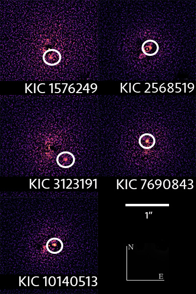
Figure 12: Robo-AO i'-band PSF-subtracted images of discovered candidate companion systems.

References

- Astropy Collaboration et al. (2013) Astropy Collaboration, Robitaille, T. P., Tollerud, E. J., et al. 2013, A&A, 558, A33, doi: 10.1051/0004-6361/201322068
- Atkinson et al. (2017) Atkinson, D., Baranec, C., Ziegler, C., et al. 2017, AJ, 153, 25, doi: 10.3847/1538-3881/153/1/25
- Baranec et al. (2016) Baranec, C., Ziegler, C., Law, N. M., et al. 2016, AJ, 152, 18, doi: 10.3847/0004-6256/152/1/18
- Baranec et al. (2014) Baranec, C., Riddle, R., Law, N. M., et al. 2014, ApJ, 790, L8, doi: 10.1088/2041-8205/790/1/L8
- Berger et al. (2018) Berger, T. A., Huber, D., Gaidos, E., & van Saders, J. L. 2018, ApJ, 866, 99, doi: 10.3847/1538-4357/aada83
- Borucki et al. (2010) Borucki, W. J., Koch, D., Basri, G., et al. 2010, Science, 327, 977, doi: 10.1126/science.1185402
- Brown et al. (2011) Brown, T. M., Latham, D. W., Everett, M. E., & Esquerdo, G. A. 2011, AJ, 142, 112, doi: 10.1088/0004-6256/142/4/112
- Burgasser et al. (2003) Burgasser, A. J., Kirkpatrick, J. D., Reid, I. N., et al. 2003, ApJ, 586, 512, doi: 10.1086/346263
- Chaplin et al. (2011a) Chaplin, W. J., Kjeldsen, H., Christensen-Dalsgaard, J., et al. 2011a, Science, 332, 213, doi: 10.1126/science.1201827
- Chaplin et al. (2011b) Chaplin, W. J., Kjeldsen, H., Bedding, T. R., et al. 2011b, ApJ, 732, 54, doi: 10.1088/0004-637X/732/1/54
- Chaplin et al. (2011c) Chaplin, W. J., Bedding, T. R., Bonanno, A., et al. 2011c, ApJ, 732, L5, doi: 10.1088/2041-8205/732/1/L5
- Colman et al. (2017) Colman, I. L., Huber, D., Bedding, T. R., et al. 2017, MNRAS, 469, 3802, doi: 10.1093/mnras/stx1056
- Donati et al. (1997) Donati, J. F., Semel, M., Carter, B. D., Rees, D. E., & Collier Cameron, A. 1997, MNRAS, 291, 658, doi: 10.1093/mnras/291.4.658
- Fares et al. (2013) Fares, R., Moutou, C., Donati, J.-F., et al. 2013, MNRAS, 435, 1451, doi: 10.1093/mnras/stt1386
- Gaia Collaboration et al. (2018) Gaia Collaboration, Brown, A. G. A., Vallenari, A., et al. 2018, A&A, 616, A1, doi: 10.1051/0004-6361/201833051
- Gaulme et al. (2014) Gaulme, P., Jackiewicz, J., Appourchaux, T., & Mosser, B. 2014, ApJ, 785, 5, doi: 10.1088/0004-637X/785/1/5
- Hinkel et al. (2015) Hinkel, N. R., Kane, S. R., Henry, G. W., et al. 2015, ApJ, 803, 8, doi: 10.1088/0004-637X/803/1/8
- Hirsch et al. (2017) Hirsch, L. A., Ciardi, D. R., Howard, A. W., et al. 2017, The Astronomical Journal, 153, 117
- Hon et al. (2019) Hon, M., Stello, D., García, R. A., et al. 2019, MNRAS, 485, 5616, doi: 10.1093/mnras/stz622
- Huber et al. (2011) Huber, D., Bedding, T. R., Stello, D., et al. 2011, ApJ, 743, 143, doi: 10.1088/0004-637X/743/2/143
- Jensen-Clem et al. (2018) Jensen-Clem, R., Duev, D. A., Riddle, R., et al. 2018, AJ, 155, doi: 10.3847/1538-3881/aa9be6
- Joye & Mandel (2003) Joye, W. A., & Mandel, E. 2003, in Astronomical Society of the Pacific Conference Series, Vol. 295, Astronomical Data Analysis Software and Systems XII, ed. H. E. Payne, R. I. Jedrzejewski, & R. N. Hook, 489
- Kraus & Hillenbrand (2007) Kraus, A. L., & Hillenbrand, L. A. 2007, AJ, 134, 2340, doi: 10.1086/522831
- Laher et al. (2012) Laher, R. R., Gorjian, V., Rebull, L. M., et al. 2012, Publications of the Astronomical Society of the Pacific, 124, 737, doi: 10.1086/666883
- Law et al. (2014) Law, N. M., Morton, T., Baranec, C., et al. 2014, ApJ, 791, 35, doi: 10.1088/0004-637X/791/1/35
- Mathur et al. (2017) Mathur, S., Huber, D., Batalha, N. M., et al. 2017, The Astrophysical Journal Supplement Series, 229, 30, doi: 10.3847/1538-4365/229/2/30
- Pinsonneault et al. (2014) Pinsonneault, M. H., Elsworth, Y., Epstein, C., et al. 2014, ApJS, 215, 19, doi: 10.1088/0067-0049/215/2/19
- Raghavan et al. (2010) Raghavan, D., McAlister, H. A., Henry, T. J., et al. 2010, The Astrophysical Journal Supplement Series, 190, 1, doi: 10.1088/0067-0049/190/1/1
- Schonhut-Stasik et al. (2017) Schonhut-Stasik, J. S., Baranec, C., Huber, D., et al. 2017, ApJ, 847, 97, doi: 10.3847/1538-4357/aa886f
- Smithsonian Astrophysical Observatory (2000) Smithsonian Astrophysical Observatory. 2000, SAOImage DS9: A utility for displaying astronomical images in the X11 window environment. http://ascl.net/0003.002
- Soubiran et al. (2013) Soubiran, C., Jasniewicz, G., Chemin, L., et al. 2013, A&A, 552, A64, doi: 10.1051/0004-6361/201220927
- Themeßl et al. (2017) Themeßl, N., Hekker, S., & Elsworth, Y. 2017, in European Physical Journal Web of Conferences, Vol. 160, European Physical Journal Web of Conferences, 05009
- Tokovinin et al. (2006) Tokovinin, A., Thomas, S., Sterzik, M., & Udry, S. 2006, A&A, 450, 681, doi: 10.1051/0004-6361:20054427
- Udry et al. (2000) Udry, S., Mayor, M., Naef, D., et al. 2000, A&A, 356, 590
- Wenger et al. (2000) Wenger, M., Ochsenbein, F., Egret, D., et al. 2000, A&AS, 143, 9, doi: 10.1051/aas:2000332
- Yu et al. (2018) Yu, J., Huber, D., Bedding, T. R., et al. 2018, ApJS, 236, 42, doi: 10.3847/1538-4365/aaaf74
- Ziegler et al. (2016) Ziegler, C., Law, N. M., Baranec, C., et al. 2016, SPIE, 9909, 99095U, doi: 10.1117/12.2231185
- Ziegler et al. (2018a) —. 2018a, AJ, 155, 161, doi: 10.3847/1538-3881/aab042
- Ziegler et al. (2018b) —. 2018b, AJ, 156, 83, doi: 10.3847/1538-3881/aace59
- Ziegler et al. (2018) Ziegler, C., Law, N. M., Baranec, C., et al. 2018, The Astronomical Journal, 156, 259