Magnetohydrodynamic Seismology of Quiet Solar Active Regions

Abstract

The ubiquity of recently discovered low-amplitude decayless kink oscillations of plasma loops allows for the seismological probing of the corona on a regular basis. In particular, in contrast to traditionally applied seismology which is based on the large-amplitude decaying kink oscillations excited by flares and eruptions, decayless oscillations can potentially provide the diagnostics necessary for their forecasting. We analysed decayless kink oscillations in several distinct loops belonging to active region NOAA 12107 on 10 July 2010 during its quiet time period, when it was observed on the West limb in EUV by the Atmospheric Imaging Assembly on-board Solar Dynamics Observatory. The oscillation periods were estimated with the use of the motion magnification technique. The lengths of the oscillating loops were determined within the assumption of its semicircular shape by measuring the position of their foot-points. The density contrast in the loops was estimated from the observed intensity contrast accounting for the unknown spatial scale of the background plasma. The combination of those measurements allows us to determine the distribution of kink and Alfvén speeds in the active region. Thus, we demonstrate the possibility to obtain seismological information about coronal active regions during the quiet periods of time.

1 Introduction

Active regions of the solar corona are regions of the enhanced plasma density penetrated by a closed magnetic field. In the Extreme Ultraviolet (EUV) band, active regions are seen as localised bundles of bright plasma loops that are believed to highlight certain magnetic flux tubes. Active regions are known to host sporadic impulsive energy releases observed as solar flares and coronal mass ejections which are the most powerful physical phenomena in the solar system. Robust forecasting of flares and mass ejections is an important element of space weather research. The key required parameter is the magnetic field. But, the direct observational measurement of the coronal magnetic field is possible in some specific cases only, because of the intrinsic difficulties connected with the high temperature and low concentration of the coronal plasma. One promising indirect method for obtaining information about the coronal magnetic field is magnetohydrodynamic (MHD) seismology, based on the estimation of the coronal Alfvén speed (e.g. Nakariakov & Ofman, 2001; Liu & Ofman, 2014; Wang, 2016). Similar plasma diagnostic techniques are used in laboratory plasma and Earth’s magnetospheric research (e.g., Fasoli et al., 2002; Nakariakov et al., 2016b, respectively).

A suitable seismological probe of the Alfvén speed in an active region is a kink (transverse) oscillation of a coronal loop (e.g. Roberts et al., 1984). Kink oscillations are excited by low-coronal eruptions, and decay in several oscillation cycles (e.g. Zimovets & Nakariakov, 2015). The spatially-resolving detection of the kink oscillation allowed for the interpretation of the oscillation as the fundamental harmonic of a standing $m=1$ fast magnetoacoustic mode of the coronal loop. The plausibility of this estimation is confirmed by the observationally established linear scaling of the kink oscillation period with the loop length (Goddard et al., 2016), and the variety of the oscillation periods detected in different loops belonging to the same bundle (Li et al., 2017). The first seismological estimation of the magnetic field in a coronal loop by a kink oscillation was performed by Nakariakov & Ofman (2001). The ratio of the wavelength that for the fundamental harmonic is double the length of the loop, and the observationally determined oscillation period gives the phase speed. As the wavelength is much longer than the minor radius of the oscillating loop, it is possible to use the theoretical estimation of the phase speed as the kink speed (Ryutov & Ryutova, 1976; Edwin & Roberts, 1983). Together with the independent estimation of the density contrast in the loop, this quantity gives the estimation of the local Alfvén speed. If there is an independent estimation of the plasma density in the loop, one gets the estimation of the absolute value of the field. An important advantage of MHD seismology by kink oscillations is a clear association of the observed oscillation with a specific plasma structure, which makes the diagnostics free of the line-of-sight integration shortcomings. Moreover, seismology allows for estimating the Alfvén speed and field in off-limb active regions where the field could not be determined by extrapolation.

In addition, the detection of multi-modal kink oscillations has led to the development of kink-based seismological techniques for the estimation of the relative density stratification, based on the ratios of the periods of different harmonics (e.g. Andries et al., 2005; Van Doorsselaere et al., 2007). The transverse profile of the density in the loop could be estimated with the use of another observable parameter, the damping time (e.g. Van Doorsselaere et al., 2004). Serious progress in coronal seismology by kink oscillations has recently been achieved with the application of the Bayesian statistics (Arregui et al., 2015; Goddard et al., 2018), see, also, (Arregui, 2018) for a recent review. An important tool for testing the theoretical results against observations is forward modelling of observables (Yuan & Van Doorsselaere, 2016a, b). The observed combination of two damping regimes, the exponential and Gaussian regimes (Pascoe et al., 2012), allowed for the development of seismological techniques for the estimation of the transverse profile of the plasma density in the oscillating loop (Pascoe et al., 2018, 2016, 2019), and its evolution in the course of the oscillation (Goddard et al., 2018). Certain theoretical shortcomings of the latter techniques have recently been discussed in (Arregui & Goossens, 2019). However, the main disadvantage of the seismology by decaying kink oscillations is their occurrence after an impulsive energy release, usually the low coronal eruption (Zimovets & Nakariakov, 2015), which excites the oscillations. This intrinsic difficulty does not allow for the diagnostics of the plasma before the eruption, which would be of interest in the context of space weather forecasting.

Another, decayless regime of kink oscillations was discovered by Wang et al. (2012). Oscillations of this kind are a ubiquitous and persistent feature of “quiet” active regions (Anfinogentov et al., 2013, 2015), i.e. they appear in the non-active periods of time. Typical oscillation periods are from a few to several minutes. The periods are found to scale linearly with the length of the oscillating loop, justifying their interpretation as standing kink modes of coronal loops. Moreover, Nisticò et al. (2013) demonstrated that the same loop oscillates in different periods of time in both decay and decayless regimes with the same oscillation period. Oscillations of this type are possibly detected in flaring loops too (Li et al., 2018), and could explain persistent oscillatory variations of the Doppler shift detected in EUV spectral observations by Tian et al. (2012). The mechanisms responsible for the sustainability of the oscillations, i.e., counteracting the damping by, e.g., resonant absorption, and hence determining the oscillation amplitude are still debated (e.g. Hindman & Jain, 2014; Murawski et al., 2015; Nakariakov et al., 2016a; Antolin et al., 2016; Guo et al., 2019; Karampelas et al., 2019). An intrinsic difficulty in the observational study of decay-less kink oscillations is that their typical projected displacement amplitudes are lower than 1 Mm, and often smaller than the pixel size of available EUV imagers. Nevertheless, these oscillations are robustly detected with the use of the recently designed motion magnification technique (Anfinogentov & Nakariakov, 2016). In particular, with the use of this technique, the coexistence of the fundamental and second spatial harmonics of decay-less kink oscillations has been revealed in (Duckenfield et al., 2018). The persistent occurrence of decay-less kink oscillations in coronal active regions before flares and eruptions makes them a promising seismological tool that can provide us with important input parameters for space weather forecasting techniques.

In this paper, we present the first seismological diagnostics of the Alfvén speed in an active region during a non-flaring period of time, i.e., in a quiet active region.

2 Observations

For our study, we selected active region NOAA 12107 observed on the West limb of the Sun on 10 July 2010. The active region was seen as a set of coronal loops of different heights, lengths and orientations. Several loops are seen to be well contrasted in the 171 Å channel. We use a 3 hours series of SDO/AIA images recorded from 14:00 UT till 17:00 UT. No flares or eruptions were observed in the active region or its vicinity during this time interval. The images were downloaded from the SDO data processing centre (http://jsoc.stanford.edu/) with the use of the provided on-line service for cutting out the region of interest. As the analysed active region was located on the solar limb, there was no need for its tracking or derotation. For the detailed analysis, we selected eight coronal loops indicated in Figure 1 with dashed lines of different colours. In Figure 1, we show an EUV image of the active region NOAA 12107 taken on 10 July 2014 at 14:32 UT.

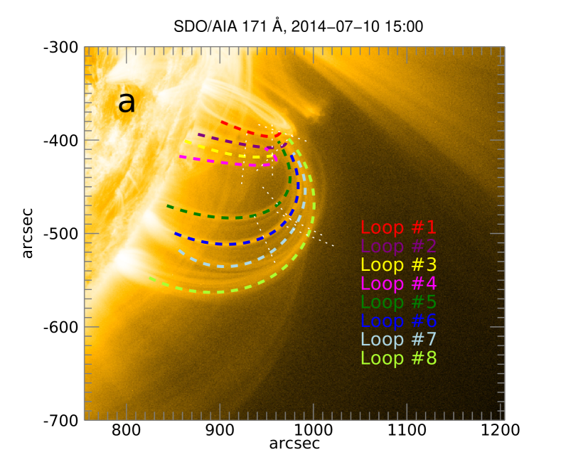
Figure 1: The EUV image of AR 12107 observed by SDO/AIA at 171 Å  on 10 July 2014 at 14:32 UT (background). Coronal loops selected for the analysis are over-plotted with the coloured dashed lines. Artificial slits used for creating time-distance plots are marked with the straight dotted lines.

3 Data analysis

3.1 Detecting oscillations using motion magnification

Decayless kink oscillations are obseved to have the displacement amplitude of the order of 0.2 Mm (Anfinogentov et al., 2015) which is less than the pixel size of SDO/AIA. The analysis of the osillations was performed by processing the imaging data cubes using the motion magnification technique (Anfinogentov & Nakariakov, 2016) based on the Dual Complex Wavelet Transform (D$\mathbb{C}$WT). Each image is decomposed into a set of complex wavelet components corresponding to different spatial scales, positions and orientations. The phase of the complex wavelet coefficients reflects the spatial location of different structures in the image and is sensitive to very small displacements of these structures in the next image. So, the algorithm tracks variations of the phase, and amplifies it in a certain broad range of periods. Performing the inverse D$\mathbb{C}$WT, we obtain a new series of images where all spatial displacements are magnified by a prescribed factor which is called the magnification coefficient.

In this work, we use the magnification coefficient of 5. We found this value optimal for our data-set, since it makes the transverse oscillations well visible in time-distance maps in the well-contrasted loops on one hand, and does not introduce significant distortion to the images on the other hand.

3.2 Time-distance maps

To make a time-distance map for an oscillating loop, we choose the instance of time where the loop has the best contrast in the 171 Å channel, and put an artificial slit across the loop near its apex. The slit position and width were manually selected individually for each loop to make the observed oscillation more evident. The slit positions are indicated in Figure 1, and their widths are listed in Table 1. In Figure 2, we show time-distance maps obtained with the use of this technique for the selected loops. The motion magnification allowed us to make the oscillatory patterns clearly visible in time distance maps for all eight loops.

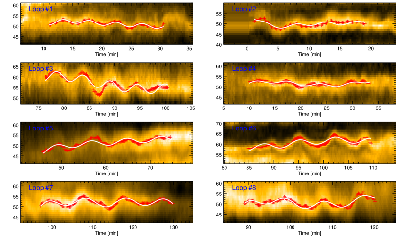
Figure 2: The time distance plots show decay-less kink oscillations observed in eight loops selected in AR 12107. The kink (transverse) motions in the image sequence were magnified by the factor of 5. The instant of time when the loops appear to be best contrasted in 171 Å images are marked with vertical green lines. Images taken at these times were used as a reference to estimate the length of the loops.

3.3 Estimation of the density contrast using Bayesian inference

To estimate the density contrast inside and outside the oscillating loop, we assume that the loop and its neighbourhood are isothermal, and the observed emission is optically thin. Thus, we model the density profile by a step function

$${\textstyle n(r)=\begin{cases}n_{0},&r<l_{0}\\ n_{\mathrm{e}},&l_{0}<r<l_{\mathrm{e}}\\ 0,&r>l_{\mathrm{e}}\end{cases}},$$ (1)

where $n_{0}$ and $n_{\mathrm{e}}$ are number densities inside and outside the loop, respectively; $l_{0}$ is the column depth of the loop segment, connected with the minor radius of the loop, and $l_{\mathrm{e}}$ is the column depth of the background plasma along the line of sight. The value of $l_{\mathrm{e}}$ is expected to be much longer than the minor radius of the loop, i.e., comparable to the active region size. Note that the estimation of the kink speed requires the value of the external number density $n_{e}$ in the vicinity of the loop. The parameter $l_{\mathrm{e}}$ is introduced to account for the emitting plasma located along the line of sight ahead and behind the oscillating loop.

Within this model the EUV intensity of the loop, $I_{0}$, and the background, $I_{\mathrm{e}}$, are calculated as

$$I_{\mathrm{e}}=G(\lambda,T)l_{\mathrm{e}}(\eta n_{0})^{2},$$ (2)

$$I_{0}=G(\lambda,T)\left[(l_{\mathrm{e}}-l_{0})(\eta n_{0})^{2}+l_{0}n_{0}^{2}\right],$$ (3)

where $\eta=n_{\mathrm{e}}/n_{0}$ is the density contrast and $G(\lambda,T)$ is the contribution function that depends upon the observed wavelength and the temperature of the emitting plasma, and accounts for specific properties of the instrument (e.g. SDO/AIA). In our case, we model only the dependence of the intensity contrast upon the density contrast and, therefore, are not interested in the absolute values. Thus, for an isothermal plasma, we can safely take $G(\lambda,T)=1$ and $l_{0}=1$.

To estimate the density contrast from the observed intensities $\mathfrak{I}_{0}$ and $\mathfrak{I}_{\mathrm{e}}$, which are the modelled intensities $I_{0}$ and ${I}_{\mathrm{e}}$ contaminated by the noise, we use the Bayesian analysis in combination with Markov Chain Monte-Carlo (MCMC) sampling. In our model, we assume that the measurement errors are normally distributed and independent in different pixels, obtaining the likelihood function,

$$P(\mathfrak{I}_{0},\mathfrak{I}_{\mathrm{e}}|\theta)=\frac{\exp{\frac{-\left[\mathfrak{I}_{\mathrm{e}}-I_{\mathrm{e}}(\theta)\right]^{2}}{\sigma_{\mathrm{e}}}}\exp{\frac{-\left[\mathfrak{I}_{0}-I_{0}(\theta)\right]^{2}}{\sigma_{0}}}}{2\pi\sigma_{\mathrm{e}}\sigma_{0}},$$ (4)

where $\theta=[n_{0},\eta,l_{\mathrm{e}}]$ is the set of free model parameters, $\sigma_{0}$, and $\sigma_{\mathrm{e}}$ are the measurement errors, and $I_{\mathrm{e}}(\theta)$ and $I_{0}(\theta)$ are the modelled intensities given by Eqs. (2) and (3). In this work, we use uniform priors with the following ranges: [0,1] for the density contrast $\eta$; [10, 200] for the background length scale $l_{\mathrm{e}}$; and [0,2] for the normalised internal density $n_{0}$.

The intensity values $I_{\mathrm{e}}$ and $I_{0}$ are obtained from the original SDO/AIA images (before the motion magnification) taken at the times when the oscillatory patterns shown in Figure 2 have been detected. The measurement uncertainties $\sigma_{0}$, and $\sigma_{\mathrm{e}}$ are estimated using the AIA_BP_ESTIMATE_ERROR function from the SolarSoft package (Freeland & Handy, 1998). Both the intensities and the corresponding errors were then normalised to such as $I_{0}=1$.

To sample the posterior probability distribution, we use our Solar Bayesian Analysis Toolkit (SoBAT) code which is available online at https://github.com/Sergey-Anfinogentov/SoBAT. The description of the code can be found in Pascoe et al. (2017). For each analysed loop, we generated $10^{6}$ samples and used them to find the most probable value of $\eta$. The credible intervals are defined as 5 and 95 % percentiles and correspond to the confidence level of 90 %.

3.4 Estimating the Alfvén speed

Firstly, we estimate the position of the oscillating loop at each instant of time by fitting a Gaussian to the transverse intensity profile of the loop extracted from the time-distance map. To estimate the period and the corresponding uncertainties from the obtained data points, we use the Bayesian analysis. Transverse displacements of each loop were modelled by a sinusoidal function on top of a polynomial trend. The measurement errors are assumed to be normally distributed and individually independent.

We generate $10^{6}$ samples from the posterior distribution using the SoBAT MCMC code. For all free parameters we use uniform priors. The kink speed $C_{\mathrm{k}}$ is then estimated from the oscillation period,

$$C_{\mathrm{k}}=\frac{2L}{P},$$ (5)

where $L$ is the length of the oscillating loop estimated by the apparent position of the loop footpoints and its apex in the assumption of the semicircular shape of the loop. To account for the uncertainties coming from the period measurements we computed $C_{\mathrm{k}}$ for each of $10^{6}$ samples from the posterior distribution of the oscillation period $P$. It allows us to estimate the most probable value and the credible intervals for the kink speed, and transparently trace the propagation of the estimated uncertainties in the estimation of the Alfvén speed.

The kink speed and density contrast allow us to estimate the external and internal Alfvén speeds as

$$C_{\mathrm{A0}} = C_{\mathrm{k}}/\sqrt{2/(1+\eta)},$$ (6)

$$C_{\mathrm{Ae}} = C_{\mathrm{A0}}/\sqrt{\eta},$$ (7)

respectively (e.g. Nakariakov & Ofman, 2001). The credibility of this technique was demonstrated by Verwichte et al. (2013) for decaying kink oscillations. To account for the uncertainties coming from the measurements of the density contrast $\eta$ and the oscillation period, we calculate $C_{\mathrm{Ae}}$ and $C_{\mathrm{A0}}$ for each of $10^{6}$ samples obtained with MCMC for the density contrast $\eta$ and the oscillation period $P$. The most probable values of $C_{\mathrm{Ae}}$ and $C_{\mathrm{A0}}$ are defined as the maximums of the corresponding histograms, and the 90% credible intervals are calculated as 5% and 95% percentiles.

Table 1: Estimation of the Alfvén speed by decay-less kink oscillations

Loop	Loop	Slit	Period	Intensity	Density	Kink	$C_{A0}$	$C_{Ae}$
No	length [Mm]	width [px]	[s]	contrast	contrast	speed [km/s]	[km/s]	[km/s]
1	224	1	$276^{+2.8}_{-2.5}$	0.23	$0.04^{+0.35}_{-0.03}$	$1622^{+15}_{-17}$	$1173^{+182}_{-23}$	$4313^{+7935}_{-2156}$
2	231	5	$334^{+40}_{-49}$	0.46	$0.07^{+0.40}_{-0.05}$	$1395^{+226}_{-163}$	$942^{+338}_{-35}$	$2765^{+4221}_{-1076}$
3	244	11	$321^{+11}_{-7.8}$	0.66	$0.11^{+0.52}_{-0.04}$	$1525^{+38}_{-52}$	$1140^{+240}_{-38}$	$2122^{+2156}_{-384}$
4	235	5	$382^{+18}_{-15}$	0.70	$0.12^{+0.57}_{-0.04}$	$1228^{+49}_{-58}$	$927^{+218}_{-43}$	$1549^{+1514}_{-184}$
5	292	28	$475^{+10}_{-10}$	0.50	$0.08^{+0.42}_{-0.06}$	$1229^{+26}_{-25}$	$903^{+161}_{-27}$	$1974^{+3578}_{-466}$
6	329	5	$435^{+12}_{-11}$	0.43	$0.07^{+0.43}_{-0.05}$	$1512^{+39}_{-42}$	$1110^{+201}_{-38}$	$2624^{+5352}_{-769}$
7	343	15	$580^{+6.7}_{-6.6}$	0.42	$0.06^{+0.43}_{-0.04}$	$1184^{+14}_{-14}$	$866^{+155}_{-21}$	$1948^{+4051}_{-489}$
8	391	13	$547^{+9.0}_{-8.5}$	0.26	$0.04^{+0.37}_{-0.03}$	$1429^{+22}_{-23}$	$1030^{+174}_{-19}$	$3353^{+6682}_{-1478}$

3.5 Mapping the Alfvén speed in the corona

The detection of kink oscillations in different coronal loops with different heights and lengths allows us to make spatially resolved estimates of the Alfvén speed in the active region. The estimation requires the knowledge of the loop lengths, oscillation periods corresponding to the fundamental kink mode, and the density contrasts in the oscillating loops (see Nakariakov & Ofman, 2001, and Section 3.4). The oscillation period is estimated directly from the time-distance maps, while the observed intensity contrast inside and outside the oscillating loop gives us a proxy for the density contrast. The length of the oscillating loop is estimated from the position of its foot-points.

For the eight chosen coronal loops, we estimated the internal and external Alfvén speeds and the corresponding uncertainties. Our estimates are summarised in Table 1. Note, that despite the huge uncertainty in the density contrast estimations, we successfully obtained reliable measurements of the Afvén speed inside oscillating loops with the accuracy of 15-20%. In Figure 3, we show a spatially resolved mapping of the internal Alfvén speed inferred from the decayless kink oscillations. The given values should be understood as values averaged along the oscillating loops, therefore the colour corresponding to the Alfvén speed value is evenly distributed along each loop.

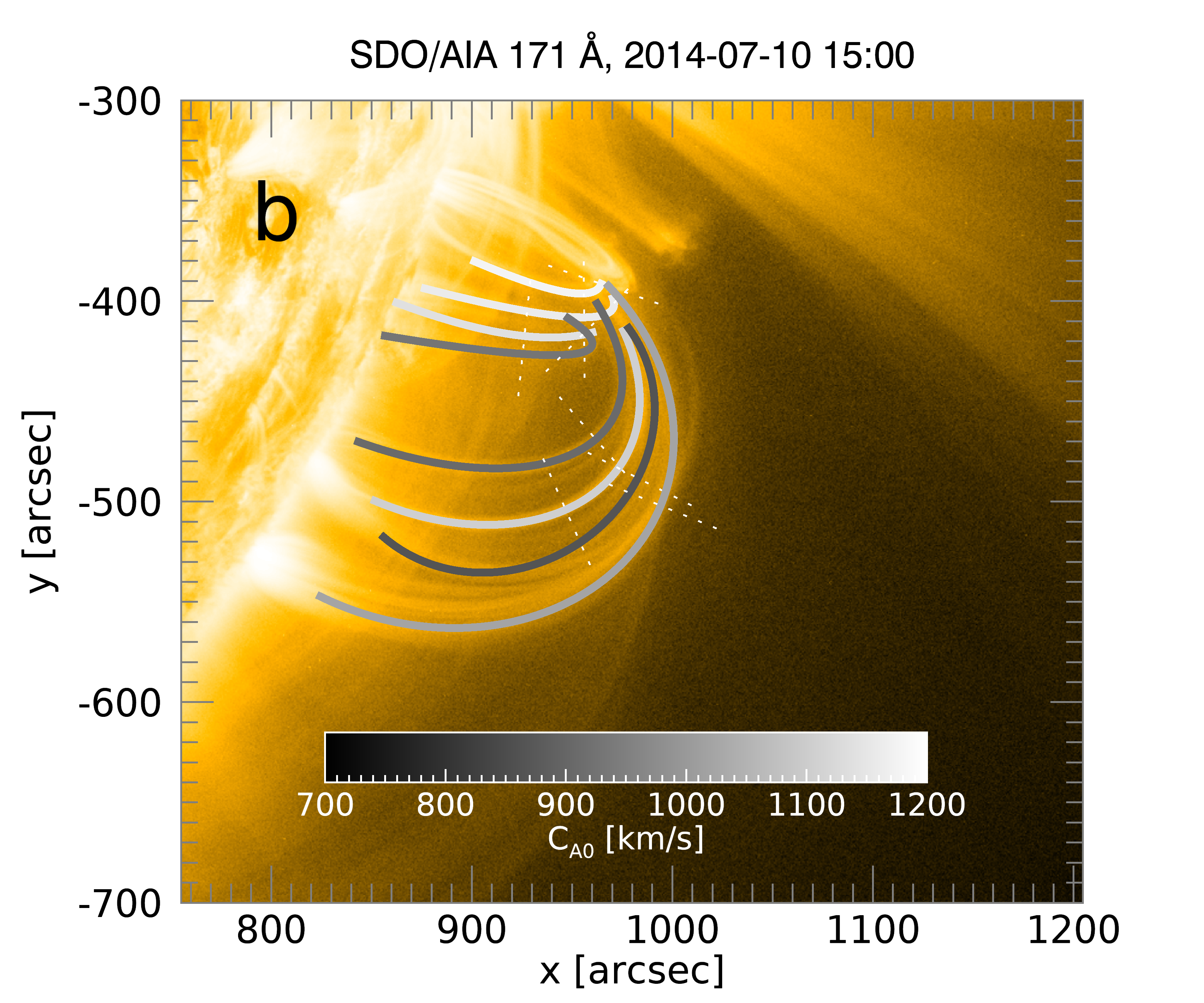
Figure 3: Mapping the Alfvén speed in AR 12107. The colour of the broad curved lines following the coronal loops show the internal Alfvén speed $C_{\mathrm{A0}}$ estimated from the observed decay-less kink oscillations. The EUV image of AR 12107 observed by SDO/AIA at 171 Å  on 10 July 2014 at 14:32 UT is used as the background. Artificial slits used for creating time-distance plots are marked with the straight dotted lines.

4 Discussion

We demonstrated that decay-less kink oscillations processed by the pioneering motion magnification technique allow one to map the Alfvén speed in the solar corona during the quiet time period. The analysis of the EUV emission from active region 12107 produced the first ever seismogram of a solar coronal active region during its quiet period, showing the spatial distribution of the Alfvén speed. The seismogram is presented in Figure 3. Note, that the quantities shown in Figure 3 correspond to the values averaged along the oscillating loops, as the effect of the plasma stratification in this study was neglected. However, further accounting for higher spatial harmonics of decayless kink oscillations (Duckenfield et al., 2018) would allow for mapping the Alfvén speed along the loops.

Relatively large errors in the estimations of the density contrast from the observed intensity contrast lead to a very uncertain estimate of the Alfvén speed in the plasma outside the loops (see Table 1). However, the Alfvén speed inside the oscillating loop can be measured with the precision of about 15–20 %. Even lower uncertainties can be achieved if more precise measurements of the density contrast are available in the same active region either spectroscopically, or by seismology based on decaying kink oscillations (e.g. Pascoe et al., 2016, 2018) . Note that the less uncertain Alfvén speed inside the oscillating loop is more informative, since it can be recalculated to the magnetic field strength after measuring independently the plasma density in the loop, while measuring the density of the background plasma is far more complicated. The density of a coronal loop can be obtained, for example, using the forward modelling approach (Goddard et al., 2018), or from the analysis of the differential emission measure (see e.g. Aschwanden et al., 2013). Even if the robust estimation of the plasma density is not possible, the estimation of the Alfvén speed is important for, for example, understanding the interaction of global coronal waves with the active region hosting the oscillating loops (e.g. Long et al., 2017). In addition, further improvement of the method can be achieved by making more precise the estimation of the length of the oscillating loop (see, e.g. Aschwanden, 2011).

In addition, we demonstrated that decayless kink oscillations can be detected in many loops within a single active region with the use of presently available EUV images provided by SDO/AIA. This detection allows us to carry out spatially resolved measurements of the Alfvén speed and, hence, potentially, the coronal magnetic field during the quiet time periods.

We should emphasise, that the coronal seismology based on decayless kink oscillations such as presented here can be performed routinely for almost every active region observed on the Sun, since decay-less kink oscillations are a ubiquitous phenomenon (Anfinogentov et al., 2015), and are detected almost always in the most of active regions.

The obtained results may be considered as the first step towards the routine estimation of the Alfvén speed and, potentially, of the magnetic field and free magnetic energy available for the release in, in particular, pre-flaring active regions.

5 Competing interests

The authors declare that they have no conflicts of interests.

References

- Andries et al. (2005) Andries, J., Arregui, I., & Goossens, M. 2005, ApJ, 624, L57, doi: 10.1086/430347
- Anfinogentov et al. (2019) Anfinogentov, S., Nakariakov, V., & Kosak, K. 2019, DTCWT based motion magnification v0.5.0, doi: 10.5281/zenodo.3368774
- Anfinogentov & Nakariakov (2016) Anfinogentov, S., & Nakariakov, V. M. 2016, Sol. Phys., 291, 3251, doi: 10.1007/s11207-016-1013-z
- Anfinogentov et al. (2013) Anfinogentov, S., Nisticò, G., & Nakariakov, V. M. 2013, A&A, 560, A107, doi: 10.1051/0004-6361/201322094
- Anfinogentov et al. (2015) Anfinogentov, S. A., Nakariakov, V. M., & Nisticò, G. 2015, A&A, 583, A136, doi: 10.1051/0004-6361/201526195
- Antolin et al. (2016) Antolin, P., De Moortel, I., Van Doorsselaere, T., & Yokoyama, T. 2016, ApJ, 830, L22, doi: 10.3847/2041-8205/830/2/L22
- Arregui (2018) Arregui, I. 2018, Advances in Space Research, 61, 655, doi: 10.1016/j.asr.2017.09.031
- Arregui & Goossens (2019) Arregui, I., & Goossens, M. 2019, A&A, 622, A44, doi: 10.1051/0004-6361/201833813
- Arregui et al. (2015) Arregui, I., Soler, R., & Asensio Ramos, A. 2015, ApJ, 811, 104, doi: 10.1088/0004-637X/811/2/104
- Aschwanden (2011) Aschwanden, M. J. 2011, Living Reviews in Solar Physics, 8, 5, doi: 10.12942/lrsp-2011-5
- Aschwanden et al. (2013) Aschwanden, M. J., Boerner, P., Schrijver, C. J., & Malanushenko, A. 2013, Sol. Phys., 283, 5, doi: 10.1007/s11207-011-9876-5
- Duckenfield et al. (2018) Duckenfield, T., Anfinogentov, S. A., Pascoe, D. J., & Nakariakov, V. M. 2018, ApJ, 854, L5, doi: 10.3847/2041-8213/aaaaeb
- Edwin & Roberts (1983) Edwin, P. M., & Roberts, B. 1983, Sol. Phys., 88, 179, doi: 10.1007/BF00196186
- Fasoli et al. (2002) Fasoli, A., Testa, D., Sharapov, S., et al. 2002, Plasma Physics and Controlled Fusion, 44, B159, doi: 10.1088/0741-3335/44/12B/312
- Freeland & Handy (1998) Freeland, S. L., & Handy, B. N. 1998, Sol. Phys., 182, 497, doi: 10.1023/A:1005038224881
- Goddard et al. (2018) Goddard, C. R., Antolin, P., & Pascoe, D. J. 2018, ApJ, 863, 167, doi: 10.3847/1538-4357/aad3cc
- Goddard et al. (2016) Goddard, C. R., Nisticò, G., Nakariakov, V. M., & Zimovets, I. V. 2016, A&A, 585, A137, doi: 10.1051/0004-6361/201527341
- Guo et al. (2019) Guo, M., Van Doorsselaere, T., Karampelas, K., et al. 2019, ApJ, 870, 55, doi: 10.3847/1538-4357/aaf1d0
- Hindman & Jain (2014) Hindman, B. W., & Jain, R. 2014, ApJ, 784, 103, doi: 10.1088/0004-637X/784/2/103
- Karampelas et al. (2019) Karampelas, K., Van Doorsselaere, T., Pascoe, D. J., Guo, M., & Antolin, P. 2019, Frontiers in Astronomy and Space Sciences, 6, 38, doi: 10.3389/fspas.2019.00038
- Li et al. (2018) Li, D., Yuan, D., Su, Y. N., et al. 2018, A&A, 617, A86, doi: 10.1051/0004-6361/201832991
- Li et al. (2017) Li, H., Liu, Y., & Vai Tam, K. 2017, ApJ, 842, 99, doi: 10.3847/1538-4357/aa7677
- Liu & Ofman (2014) Liu, W., & Ofman, L. 2014, Sol. Phys., 289, 3233, doi: 10.1007/s11207-014-0528-4
- Long et al. (2017) Long, D. M., Bloomfield, D. S., Chen, P. F., et al. 2017, Sol. Phys., 292, 7, doi: 10.1007/s11207-016-1030-y
- Murawski et al. (2015) Murawski, K., Solov’ev, A., Kraśkiewicz, J., & Srivastava, A. K. 2015, A&A, 576, A22, doi: 10.1051/0004-6361/201424684
- Nakariakov et al. (2016a) Nakariakov, V. M., Anfinogentov, S. A., Nisticò, G., & Lee, D.-H. 2016a, A&A, 591, L5, doi: 10.1051/0004-6361/201628850
- Nakariakov & Ofman (2001) Nakariakov, V. M., & Ofman, L. 2001, A&A, 372, L53, doi: 10.1051/0004-6361:20010607
- Nakariakov et al. (2016b) Nakariakov, V. M., Pilipenko, V., Heilig, B., et al. 2016b, Space Sci. Rev., 200, 75, doi: 10.1007/s11214-015-0233-0
- Nisticò et al. (2013) Nisticò, G., Nakariakov, V. M., & Verwichte, E. 2013, A&A, 552, A57, doi: 10.1051/0004-6361/201220676
- Pascoe et al. (2017) Pascoe, D. J., Anfinogentov, S., Nisticò, G., Goddard, C. R., & Nakariakov, V. M. 2017, A&A, 600, A78, doi: 10.1051/0004-6361/201629702
- Pascoe et al. (2018) Pascoe, D. J., Anfinogentov, S. A., Goddard, C. R., & Nakariakov, V. M. 2018, ApJ, 860, 31, doi: 10.3847/1538-4357/aac2bc
- Pascoe et al. (2016) Pascoe, D. J., Goddard, C. R., Nisticò, G., Anfinogentov, S., & Nakariakov, V. M. 2016, A&A, 589, A136, doi: 10.1051/0004-6361/201628255
- Pascoe et al. (2012) Pascoe, D. J., Hood, A. W., de Moortel, I., & Wright, A. N. 2012, A&A, 539, A37, doi: 10.1051/0004-6361/201117979
- Pascoe et al. (2019) Pascoe, D. J., Hood, A. W., & Van Doorsselaere, T. 2019, Frontiers in Astronomy and Space Sciences, 6, 22, doi: 10.3389/fspas.2019.00022
- Roberts et al. (1984) Roberts, B., Edwin, P. M., & Benz, A. O. 1984, ApJ, 279, 857, doi: 10.1086/161956
- Ryutov & Ryutova (1976) Ryutov, D. A., & Ryutova, M. P. 1976, Soviet Journal of Experimental and Theoretical Physics, 43, 491
- Tian et al. (2012) Tian, H., McIntosh, S. W., Wang, T., et al. 2012, ApJ, 759, 144, doi: 10.1088/0004-637X/759/2/144
- Van Doorsselaere et al. (2004) Van Doorsselaere, T., Andries, J., Poedts, S., & Goossens, M. 2004, ApJ, 606, 1223, doi: 10.1086/383191
- Van Doorsselaere et al. (2007) Van Doorsselaere, T., Nakariakov, V. M., & Verwichte, E. 2007, A&A, 473, 959, doi: 10.1051/0004-6361:20077783
- Verwichte et al. (2013) Verwichte, E., Van Doorsselaere, T., Foullon, C., & White, R. S. 2013, ApJ, 767, 16, doi: 10.1088/0004-637X/767/1/16
- Wang et al. (2012) Wang, T., Ofman, L., Davila, J. M., & Su, Y. 2012, ApJ, 751, L27, doi: 10.1088/2041-8205/751/2/L27
- Wang (2016) Wang, T. J. 2016, Washington DC American Geophysical Union Geophysical Monograph Series, 216, 395, doi: 10.1002/9781119055006.ch23
- Wareham et al. (2017) Wareham, R., Cotter, F., scf32, et al. 2017, rjw57/dtcwt: Version 0.12.0, doi: 10.5281/zenodo.889246
- Yuan & Van Doorsselaere (2016a) Yuan, D., & Van Doorsselaere, T. 2016a, ApJS, 223, 23, doi: 10.3847/0067-0049/223/2/23
- Yuan & Van Doorsselaere (2016b) —. 2016b, ApJS, 223, 24, doi: 10.3847/0067-0049/223/2/24
- Zimovets & Nakariakov (2015) Zimovets, I. V., & Nakariakov, V. M. 2015, A&A, 577, A4, doi: 10.1051/0004-6361/201424960