Stochastic Triangular Mesh Mapping:
A Terrain Mapping Technique for Autonomous Mobile Robots

Abstract

For mobile robots to operate autonomously in general environments, perception is required in the form of a dense metric map. For this purpose, we present the *STM mapping technique: a 2.5-D representation of the surface of the environment using a continuous mesh of triangular surface elements, where each surface element models the mean plane and roughness of the underlying surface. In contrast to existing mapping techniques, *STM map models the structure of the environment by ensuring a continuous model, while also being able to be incrementally updated with linear computational cost in the number of measurements. We reduce the effect of uncertainty in the robot pose (pose) by using landmark-relative submaps. The uncertainty in the measurements and robot pose are accounted for by the use of Bayesian inference techniques during the map update. We demonstrate that *STM map can be used with sensors that generate point measurements, such as *LiDAR sensors and stereo cameras. We show that *STM map is a more accurate model than the only comparable online surface mapping technique—a standard elevation map—and we also provide qualitative results on practical datasets.

Graphical Abstract

Highlights

• A novel dense mapping technique that uses a stochastic triangular mesh is presented.

• The technique handles uncertainty from multiple sources in a principled manner.

• The map models the structure in the environment while remaining tractable to update.

• The inference algorithm employs a novel combination of message passing techniques.

• The mapping technique is tested on a large-scale practical dataset.

[2]~δ^*_#1 ←#2 [2]~δ^*_#1 →#2 ./figs/ SLAM short=SLAM, long=simultaneous localisation and mapping SPLAM short=SPLAM, long=simultaneous planning, localisation and mapping LiDAR short=LiDAR, long=light detection and ranging IRF short=IRF, long=inertial reference frame BRF short=BRF, long=body reference frame PGM short=PGM, long=probabilistic graphical model BP short=BP, long=belief propagation LBP short=LBP, long=loopy belief propagation LBU short=LBU, long=loopy belief update surfel short=surfel, long=surface element voxel short=voxel, long=volumetric element pose short=pose, long=position and orientation NDT short=NDT, long=normal distributions transform GP short=GP, long=Gaussian process, long-plural=es SDF short=SDF, long=signed distance function TSDF short=TSDF, long=truncated signed distance function MLS short=MLS, long=multi-level surface PML short=PML, long=probabilistic multi-level ROC short=ROC, long=receiver operating characteristic BCM short=BCM, long=Bayesian committee machine UT short=UT, long=unscented transform RKHS short=RKHS, long=reproducing kernel Hilbert space KL short=KL, long=Kullback-Leibler EP short=EP, long=expectation propagation VMP short=VMP, long=variational message passing IID short=IID, long=independently and identically distributed STM short=STM, long=stochastic triangular mesh, short-indefinite=an, long-indefinite=a HYMM short=HYMM, long=hybrid metric map MCMC short=MCMC, long=Markov chain Monte Carlo MAP short=MAP, long=maximum a posteriori MSE short=MSE, long=mean squared error, short-indefinite=an, long-indefinite=a DGPS short=DGPS, long=differential global positioning system LIBELAS short=LIBELAS, long=library for efficient large-scale stereo matching MRF short=MRF, long=Markov random field DAG short=DAG, long=directed acyclic graph KF short=KF, long=Kalman filter EKF short=EKF, long=extended Kalman filter UKF short=UKF, long=unscented Kalman filter LM short=LM, long=Levenberg-Marquardt PnP short=PnP, long=Perspective-n-Point IMU short=IMU, long=inertial measurement unit EMDW short=EMDW, long=elementary, my dear Watson

left=25mm,right=25mm,top=25mm,bottom=20mm

left=25mm,right=25mm,top=25mm,bottom=25mm

1 Introduction

For an autonomous mobile robot to operate effectively, it needs the ability to perceive its environment; this problem of perception is commonly referred to as mapping. More precisely, mapping can be defined as representing a robot’s belief over the environment, where “belief” refers to the knowledge about a state, given all measurements and any prior information. In the general case of a robot operating in an initially unknown environment, the map needs to be incrementally built online using the robot’s measurements of the environment, such that the robot can make decisions in real time. These measurements are obtained using exteroceptive sensors—typically a combination of LiDAR sensors, stereo cameras, and depth-cameras. In order to perform complex tasks—such as path planning, collision detection, or object manipulation—a 3-D dense metric map is required. Guizilini and Ramos [1] argue that, for a dense metric map to be an effective representation, it should have the following attributes:

• Reason under uncertainty. Measurements from all robot sensors contain some degree of uncertainty, which needs to be accounted for when updating the map.

• Incremental updates. Due to the online nature of the problem, all the measurements are not available at once and, as the robot needs to continuously query the map, the map needs to be updated incrementally.

• Update and query efficiently. Exteroceptive sensors generate vast amounts of data—typically in the form of dense point clouds—that need to be incorporated quickly into the map. Additionally, the resulting map needs to be accessed quickly when required.

• Represent the structure in the environment. The environment is inherently structured according to spatial relationships on various length scales. By exploiting this structure, a map can interpolate occluded regions, or better estimate regions with few measurements.

In this paper, we present STM mapping, an online dense mapping technique designed around these four attributes. In particular, we focus on two aspects:

Robot pose belief

A source of uncertainty influencing dense mapping is localisation; to build an accurate model of the environment, one must also consider the belief over the robot pose. Estimating the robot pose belief is typically performed using the process of SLAM, whereby the belief over a sparse map—consisting of re-identifiable landmarks—is estimated in conjunction with the robot pose. The sparsity of this landmark map, however, prohibits it being used for complex planning tasks, and it should therefore rather be considered as a localisation aid. When performing SLAM, the beliefs over the robot pose at any time step can change due to new information, as is also the case when a robot revisits a part of the environment—that is, when loop closure is performed. This can cause significant changes in the beliefs over these previous poses, which present a problem, as measurements obtained at previous poses would have been incorporated into the dense map using the previous pose beliefs. To account for this, measurements would need to be removed and reintegrated into the map using the retroactively updated pose beliefs—an expensive undertaking.

Statistical dependencies

An aspect of representing the structure of the environment in a map is to model the continuity of surfaces. However, most dense mapping techniques are made tractable through the assumption that neighbouring map elements are statistically independent (as we will discuss in Section 2). This allows each element to be updated independently, but at the expense of modelling continuity. As a consequence of this assumption, the resulting models contain numerous discontinuities. This is problematic for a task like collision prediction, for which it is desirable to have a continuous representation of the environment in order for it to function accurately. The alternative approach of modelling dependencies between map elements will lead to more accurate map beliefs, but at a higher computational cost.

In order to address the issue of the uncertainty in the robot pose belief, we develop the STM mapping technique using triangular submapping regions, demarcated by landmarks extracted using *SLAM—the 2-D *HYMM framework [2, 3]. In order to motivate this decision, we briefly explain the HYMM framework, and provide a 3-D extension to it (Section 3). Using this submapping framework, we then develop our STM mapping technique, representing the structure of the environment using a continuous surface (Sections 4 to 5). Finally, we present some experimental results, building STM maps using both simulated and practical data (Section 6).

2 Existing Approaches to Dense Mapping

To motivate our proposal for a new mapping technique, we now review and evaluate the existing approaches to dense mapping, and specifically consider the desired attributes a dense map should have.

2.1 Polygonal Mesh Maps

Polygonal meshes are a well-known method of spatial modelling used in computer graphics. A mesh is constructed from a point cloud by linking points together with edges, forming polygons. In an early application, Thrun et al. [4] incrementally built sections of a triangular mesh of indoor environments, subsequently simplifying areas of the mesh by fitting rectangular planes using an online implementation of expectation maximisation. More recently, Wiemann et al. [5] used a $k$-nearest-neighbours approach to estimate the normals of a triangular mesh, creating a consistent representation of planar surfaces. The resulting mesh was simplified by fusing local polygons with similar normal vectors; however, this process was calculated in post-processing. Zienkiewicz et al. [6] modelled small-scale environments with a fixed-topology triangular mesh, and formulated the update procedure probabilistically. By performing weighted optimisation, they were able to iteratively and incrementally obtain solutions to the mesh. Although their approach is formatted probabilistically, it does not capture the uncertainty in the model. Polygonal meshes are not designed to explicitly represent any uncertainty, and therefore cannot incorporate the robot pose belief or sensor uncertainty in a principled manner. They are, however, a popular method for visualising other probabilistic techniques.

2.2 Occupancy Grid Maps

Occupancy grid mapping is one of the most widely used mapping techniques and is considered the de facto representation for dense mapping. Originally developed in 2-D by Moravec and Elfes [7], this technique discretises the map into a volumetric grid, where each voxel stores the probability that the associated region is occupied. As with all volumetric representations in 3-D, spanning the mapping space with a grid becomes prohibitively expensive, despite the majority of the mapped space being either unoccupied or unobserved. To address this, Hornung et al. [8] developed the OctoMap framework—this is arguably the most used dense mapping framework. Instead of a fixed voxel size, they used octrees to recursively adjust the voxel resolution. Unimportant information, namely the unoccupied or unobserved space, is compressed into coarse voxels, while a finer resolution is maintained for occupied regions. Improving on this, Einhorn et al. [9] developed an adaptive online method of determining the division depth in local regions of the map using the more general k-d tree. Khan et al. [10] used rectangular voxels to compress unoccupied cubic voxels. In recent work, Droeschel et al. [11] used an allocentric (robot-centric) grid, where the resolution increases with the distance from the robot. Their approach was also implemented practically, and tested at the DARPA Robotics Challenge. In order to handle the uncertainty of the robot pose belief, Joubert et al. [12] incorporated a beam sensor model into occupancy map updates using Monte Carlo integration, although this approach was only demonstrated in 2-D. In an attempt to incorporate statistical dependency between 2-D voxels, Thrun [13] used a forward measurement model and, in an offline post-processing procedure, optimised for the maximum likelihood map.

Despite their popularity, occupancy grid maps fail to incorporate the dependencies between map elements in an online manner.

2.3 Elevation Maps

The most general way of representing an environment is to use a 3-D dense map; however, some environments are adequately represented as a 2.5-D map—that is, a single axis is constrained to only one value per map element. These elevation maps reduce the dimensionality of the map by associating a single height to each element of a 2-D grid. Early work by Hebert et al. [14] used an elevation map to perform localisation, as well as to identify footholds for a legged robot. A drawback of elevation maps is their inability to represent overhangs, such as bridges. Triebel et al. [15] dealt with this problem in their method of MLS mapping by clustering the measurements in each map element, with the clusters across neighbouring map elements being segmented into elevation classes. Recent work by Fankhauser et al. [16] incorporated the uncertainty in robot pose belief into an allocentric elevation map. They achieved this by maintaining a distribution over the spatial uncertainty of each cell, which is updated over time based on the uncertainty in transformations between the allocentric reference frames. The resultant map is constructed from the weighted average of neighbouring cells, based on each cell’s spatial uncertainty. Their approach was demonstrated for a legged robot. In gamma-SLAM, Marks et al. [17] represent the environment using a 2.5-D precision map, where measurements in each map element are modelled as samples from a Gaussian distribution over the elevation, with an unknown mean and precision. By considering only the precision—marginalising out the mean—their method generates accurate maps for localisation, while also providing a pseudo-metric for traversability. However, their model fails to account for the case where the sensor uncertainty varies at different ranges, and the model disregards height.

Elevation maps are an efficient and effective method of representing environments in which a full 3-D representation is unnecessary. However, elevation maps fail to incorporate the statistical dependencies between map elements.

2.4 Signed Distance Function Maps

Over the last decade, advances in depth-camera technology have created affordable and relatively accurate depth sensors. This has given rise to a non-parametric surface representation of the environment using the SDF, commonly used in computer graphics. The SDF calculates the Euclidean distance to the nearest surface, defining positive values to indicate free space and negative values to indicate occluded regions. Consequently, the surface is implicitly described at the zero-crossings. In KinectFusion, a technique pioneered by Newcombe et al. [18], measurements are fused into a regular 3-D grid of voxels, storing truncated SDF values. Due to memory constraints, this method is only suitable to medium-scale environments. Whelan et al. [19] expanded this to handle large-scale environments by using a sliding window to maintain a local section of the environment as an SDF map, while incrementally converting the regions exiting this window into a triangular mesh. A major advantage of this method is its ability to adjust the map upon a loop closure. This is achieved through an optimisation procedure over the sensor poses and vertices of the meshed map—creating a globally consistent map. BundleFusion, a method devised by Dai et al. [20], performs bundle adjustment to optimise over the sensor poses to create accurate SDF maps. Similarly to KinectFusion, this method suffers from memory constraints due to maintaining the complete map in a grid, and is therefore limited to small-scale environments. The standard SDF representation is not probabilistic, and consequently neither sensor uncertainty nor pose uncertainty can be incorporated when updating the map. To address this, Dietrich et al. [21] modelled each distance as Gaussian distributed. However, this choice of distribution can yield negative estimates for a positive-only quantity (distance).

Although SDF methods have been shown to generate highly detailed maps in real time, they have not been used widely in the robotics community due to several drawbacks. Firstly, the SDF can only implicitly describe the surfaces in the environment; when an explicit surface map is required, the SDF map needs to be converted to a mesh. Secondly, as the standard SDF representation is not probabilistic, it cannot model the statistical dependencies between mapping elements. Finally, SDF methods are limited to a single sensor type, namely depth cameras.

2.5 Normal Distribution Transform Maps

The NDT mapping model was originally developed by Biber and Strasser [22] as a method for 2-D scan matching, and then independently expanded to 3-D by Takeuchi and Tsubouchi [23], and Magnusson et al. [24]. The resulting volumetric representation maintains a 3-D Gaussian distribution in each voxel. Consequently, measurements falling within a voxel are assumed to be IID samples drawn from a Gaussian distribution, where the sufficient statistics, namely the mean and covariance, can be calculated incrementally. Stoyanov et al. [25] showed that the resulting maps are accurate spatial representations when compared with the methods of occupancy grid mapping and polygonal meshes. They analysed all the methods on simulated and real-world data, comparing ROC curves, accuracy, and runtime. NDT mapping was augmented by Saarinen et al. [26] to include the dimension of occupancy, thus creating the NDT occupancy map (NDT-OM). Their representation allows multi-resolution support for the NDT, while also introducing a temporal measure to handle dynamic environments.

Due to the IID assumption, a drawback of the NDT is that it cannot account for heterogeneous uncertainty, which is present in the sensor models and the robot pose belief. The map elements are also assumed to be statistically independent.

2.6 Gaussian Process Maps

A popular method of incorporating map element dependencies uses GP regression [27]—a method of regression using a non-parametric stochastic model. A set of input training points (measurements of the environment) are used to predict the output at some desired query points. In order to perform this regression, the correlation between points is described by a kernel (covariance), which is parameterised by a set of hyperparameters. GP can only perform regression on a 1-D output; due to this, GP were initially applied to 2.5-D elevation maps. Lang et al. [28] used an iterative, locally adaptive non-stationary kernel, which was able to handle sharp discontinuities without severe smoothing. Extending this, Plagemann et al. [29] used a separate GP to estimate the hyperparameters of each kernel. An ensemble of overlapping GP was also tiled to cover the mapping region. This method was practically applied to foothold detection of a quadruped robot. Vasudevan [30] implemented a dependent GP to perform offline large-scale terrain modelling on scans of an open mine. Hadsell et al. [31] used a non-stationary kernel of which the hyperparameters were a function of the uncertainty of the measurement range.

In order to use GP regression in full 3-D space, the environment needs to be described implicitly; one method of doing this uses occupancy. Occupancy maps in the context of GP mapping were first proposed by O’Callaghan and Ramos [32], who developed a framework for constructing 2-D GP occupancy maps (GPOMs). To determine the probability of occupancy, an additional probabilistic least-squares classifier was used. This method was able to incorporate uncertainty in the sensor measurements and the robot pose into the map using the unscented transform and Gauss-Hermite quadrature. Jadidi et al. [33] improved on GPOMs by considering the case in which the pose uncertainty is significant, and incorporated this uncertainty into a warped GPOM representation using Gauss-Hermite quadrature and Monte Carlo integration. Both these methods, however, were offline post-processing procedures.

The standard GP formulation cannot be applied to online mapping due to two main issues. Firstly, it is required that all the training data be available at once. Secondly, performing online GP regression is intractable due the cubic computational complexity in the amount of training data. An approximate method of addressing both of these issues is to partition the training data using a BCM [34], which is a method of combining estimators trained on different data by assuming conditional independence. BCMs have a linear computational complexity in the partition size and have been shown to decrease computational time—matching that of even the OctoMap framework [35, 36]. This method, however, combines multiple independently trained estimators, which is an inaccurate representation of the map belief.

Although GP do not assume statistical independence between map elements, this comes at a prohibitive computational cost and, for this reason, GP have primarily been limited to offline mapping. Their performance is also largely dependent on suitable hyperparameters, which can require optimisation throughout the mapping process. The resulting map is also a jointly Gaussian distribution over all the query points, which can become prohibitively expensive to maintain.

2.7 Hilbert Maps

A more recent method of incorporating the dependencies between map elements was introduced by Ramos and Ott [37]. Their approach, Hilbert maps, aims to generate a continuous occupancy representation of the environment. To achieve this, spatial measurements are projected onto a high-dimensional feature space, in which a simple linear classifier, namely logistic regression, is incrementally trained using stochastic gradient descent. The resulting representation is a parametric occupancy map of the environment. The robot pose belief and sensor uncertainties are also incorporated into the features using numerical integration. To improve efficiency, Doherty et al. [38] used the approach of fusing local maps, whereby multiple logistic regression classifiers could be combined incrementally. Guizilini and Ramos [1] proposed an efficient Hilbert maps approach by clustering measurements to decrease the dimensionality of the feature vectors. This efficient extension to the Hilbert maps framework was able to achieve training speeds rivalling that of the OctoMap framework. However, as a grid is not specified during training, this results in significantly poorer performance when querying the map in comparison to OctoMap.

Hilbert maps do not represent the uncertainty in the resulting map and therefore cannot truly be considered a probabilistic representation of the environment. The Hilbert maps framework has also only been demonstrated using accurate LiDAR sensors, and whether the approximations made will expand for less accurate sensors—like stereo cameras—is unclear.

2.8 Evaluation

The main attributes of the existing mapping techniques are summarised in Table 1. We also include our proposed mapping technique—STM mapping. From this we highlight a few important points related to the existing techniques:

Table 1: Comparison of the different dense mapping techniques across different attributes. We also show our STM mapping technique for comparison.

Mapping Technique	Incorporate Uncertainty	Incremental Updates	Update Efficiency	Statistical Dependencies	Explicit Surface
Polygonal Mesh	✗	✗	$\mathcal{O}(N)$	✗	✓
Occupancy Grid	✓	✓	$\mathcal{O}(N)$	✗	✗
Elevation	✓	✓	$\mathcal{O}(N)$	✗	✓
SDF	✗	✓	$\mathcal{O}(N)$	✗	✗
NDT	Not in measurements	✓	$\mathcal{O}(N)$	✗	✓
GP	✓	✗	$\mathcal{O}(N^{3})$	✓	✓
Hilbert	Not in the map	✓	$\mathcal{O}(N)$	✓	✗
STM	✓	✓	$\mathcal{O}(N)$	✓	✓

Robot pose belief uncertainty

The majority of probabilistic mapping techniques—bar NDT mapping—have the ability to account for the uncertainty in the robot pose belief by marginalising it out using numerical integration; this increases the uncertainty in the measurements, consequently increasing the map uncertainty. Although this represents the belief over the environment more accurately, if the uncertainty in the robot pose belief is significant, this could render the map essentially useless. Additionally, marginalising out the robot pose belief removes the dependencies between poses. This is again a problem when there are significant changes in the beliefs over previous poses, as the affected areas of the map need to be recalculated. A popular approach to alleviate these issues is to perform submapping, which we discuss in depth later (Section 3).

Statistical dependencies

Most existing mapping techniques cannot incorporate statistical dependencies between map elements. Of the two main techniques that can, GP mapping comes at an intractable computational cost, and Hilbert maps do not capture any uncertainty in the resulting map, which does not accurately model the belief over the environment. In STM mapping, we enforce continuity in the model, which causes statistical dependencies between map elements; however, this only comes at a linear computational cost and still maintains a probabilistic map (Section 4).

Explicit surface models

The existing dense mapping techniques either model the underlying surfaces in the environment explicitly or implicitly. An explicit surface representation is arguably more useful, because some methods of collision prediction [40, 41] require an explicit surface representation. An explicit surface can be extracted from an implicit surface representation; however, this requires an extra step of computation, and results in a model which does not represent any surface uncertainty. For example, an occupancy grid map could be converted to an explicit surface by thresholding the probability of occupancy. We therefore opt for an explicit surface representation of the environment (Section 4).

Incremental updates

Being able to incrementally update the map is critical for online operation. However, to produce an accurate map belief, it is just as important to use Bayesian reasoning when updating the map incrementally. Specifically, the map’s current state—based on prior measurements—should be considered as context when fusing new measurements into the map; that is, we should use Bayes’ theorem. The probabilistic techniques that use incremental Bayesian updates—occupancy grid, elevation, and NDT maps—do not incorporate statistical dependencies. Despite being a Bayesian technique, GP maps require the BCM approximation to perform incremental updates, and this approximation neglects the map’s current state when updating. Additionally, the Hilbert maps method cannot represent the uncertainty in its estimates of the map, as it follows a frequentist approach. In STM mapping, we incorporate incremental Bayesian updates into a continuous representation of the environment (Section 4).

Given our evaluation of the existing dense mapping techniques and the comparison to our proposed technique (Table 1), we believe that the *STM mapping technique constitutes a valuable contribution to the field of dense mapping for mobile robots. In the remainder of this paper, we develop and test the STM mapping technique.

3 Inertial Reference Frames in Dense Mapping

The uncertainty in the robot pose belief is ever present when performing online dense mapping. If the robot pose belief contains significant uncertainty, it creates problems when incorporating measurements into the dense map. In this chapter, we explore submapping—an approach that reduces the effect of the uncertainty in the robot pose belief—and motivate our choice of submapping framework in the STM mapping technique.

All robotic systems are described in terms of IRF. When discussing the issue of the uncertainty in the robot pose belief in dense mapping, it is important to understand the effect that the choice of IRF has on the resulting map. Some mapping techniques have used an allocentric IRF to ensure that the region of the map currently surrounding the robot has lower uncertainty [16] or a finer grid resolution [11]. In contrast, most mapping techniques focus on building globally consistent maps in a fixed, single-privileged IRF—often referred to as a global IRF. Due to the compounding effect of uncertain motion on the robot pose belief, regions of the map further away from the origin of the chosen IRF are increasingly uncertain; in the absence of absolute position sensing, this uncertainty is unbounded. Furthermore, when performing SLAM in a global IRF and then performing loop closure, large changes in beliefs over previous robot poses can be induced. Despite this, the relative uncertainty between successive robot poses is bounded by the—typically confident—motion dynamics. The submapping approach takes advantage of this by segmenting the environment into several submaps, each with its own IRF. This approach is used in some of the recent state-of-the-art vision-based SLAM techniques, namely LSD-SLAM by Engel et al. [42], and ORB-SLAM by Mur-Artal and Tardós [43]; both of these techniques use keyframes as intermediate submaps during SLAM. In the case of dense mapping in indoor environments, the map can be semantically segmented by room [44]. In general environments, a typical method of defining submaps uses overlapping rectangular cuboids to span the mapping space [45, 46]. However, this causes two issues: the map contains redundant regions, and it is non-trivial to accurately describe new measurements in terms of the IRF of previously observed submaps. HYMM [2, 3] is a 2-D submapping technique that addresses both of these issues by using relative IRF based on the sparse landmark map obtained from SLAM. In Section 3.1, we review the HYMM framework and present a 3-D extension to it. Utilising this framework, we present a principled method of decoupling measurements of the environment from the robot pose belief (Section 3.2).

Notational remark

A point in the global IRF, $\bm{x}$, is expressed in the BRF of the robot as $\bm{x}^{B}$, and in a relative IRF as $\bm{x}^{R}$.

3.1 Relative Inertial Reference Frames

The HYMM submapping technique segments the environment by constructing a triangular mesh between selected landmarks (Figure 1a). A relative IRF is associated with each triangular submap, defined in terms of the three landmarks at the vertices of the triangular region. To elucidate this definition, consider a submap demarcated by the convex hull of the landmarks $\bm{l}_{0}$, $\bm{l}_{\alpha}$ and $\bm{l}_{\beta}$. A 2-D point, $\bm{m}$, in the global IRF can be described by

$$\begin{split}\bm{m}&=\alpha(\bm{l}_{\alpha}-\bm{l}_{0})+\beta(\bm{l}_{\beta}-\bm{l}_{0})+\bm{l}_{0}\\ &=\alpha\bm{a}+\beta\bm{b}+\bm{l}_{0}.\end{split}$$ (1)

For $\bm{m}$ to be within the submap, $\alpha$ and $\beta$ must satisfy

$$\alpha+\beta\leq 1\quad\text{and}\quad\alpha,\beta\in[0,1].$$ (2)

The 2-D relative IRF axes are defined by $\bm{a}$ and $\bm{b}$—$\bm{l}_{0}$ is an offset—and $(\alpha,\beta)$ are the coordinates of a 2-D point $\bm{m}$ in the relative IRF.

To extend the 2-D relative IRF of the HYMMs to 3-D, a third axis is required. One could project the 3-D landmarks onto the horizontal plane and use the vertical axis of the global IRF. However, this approach couples the relative IRF to the global IRF, negating the true benefits of a relative IRF. Guivant et al. [2] suggested—but did not develop—two ideas of extending HYMMs to 3-D. The relative IRF axes could be constructed using four landmarks, forming tetrahedral submapping regions; however, it could be impractical to adequately span the mapping space. Alternatively, the 2-D approach can be adapted to 3-D by defining the submapping region being normal to the triangular faces of the 3-D landmark mesh. We develop the latter approach, extending the relative IRF to 3-D by introducing the third axis as

$$\bm{n}=\frac{\bm{a}\times\bm{b}}{\mathinner{\!\left\lVert\bm{a}\times\bm{b}\right\rVert}}.$$ (3)

Using this definition, a 3-D point, $\bm{m}$, can be described as

$$\begin{split}\bm{m}&=\alpha\bm{a}+\beta\bm{b}+\gamma\bm{n}+\bm{l}_{0}\\ &=\begin{bmatrix}\bm{a}&\bm{b}&\bm{n}\end{bmatrix}\bm{m}^{R}+\bm{l}_{0},\end{split}$$ (4)

where $\bm{m}^{R}=\begin{bmatrix}\alpha&\beta&\gamma\end{bmatrix}^{\intercal}$ is a point in the 3-D relative IRF (Figure 1b). The constraints in Equation 2 also hold for $\bm{m}$ to fall within the submap.

(a)

(b)

Figure 1: (a) The HYMM submapping method [2, 3] segments the environment using landmarks. (b) In our 3-D extension to the HYMM representation, a point $\bm{m}$ within a submap can be fully described relative to these landmarks.

There is, however, a caveat to using this relative IRF description. As the definition of the relative IRF relies on landmarks, it is necessary for the chosen landmarks to be robustly and persistently identifiable. While this is still an open problem for general environments, given the progress that has been made in the past decade in feature and place recognition [47], we believe that this will be possible in the future. Despite this, there are practical applications, in more controlled environments, where easily identifiable landmarks could be placed manually in the environment—for example in land surveying, 3-D object reconstruction, or factory operation. We practically demonstrate an example of such an application in Section 6.4.

3.2 Decoupling Dense Measurements from the Robot Pose Belief

With the relative IRF definition in hand, we now present a method of decoupling measurements of the surface of the environment from their associated robot pose beliefs. Consequently, this method decouples the process of localisation from that of dense mapping. We achieve this decoupling by transforming surface measurements from the BRF of the robot to the relative IRF of the associated submap—as opposed to transforming to the global IRF.

We model the process of observing a point on the surface of the environment (in the BRF of the robot) using a sensor beam model, whereby a noisy measurement, $\bm{z}^{B}$, is generated by a point, $\bm{m}^{B}$, on the surface of the environment. Most sensors observe multiple environment surface points at a single time step. We denote the sequence of measurements as $\mathit{Z}^{B}=(\bm{z}^{B}_{i})$, and the associated environment surface points as $\mathit{M}^{B}=(\bm{m}^{B}_{i})$. Assuming an uninformative prior over $\mathit{M}^{B}$, we can calculate the belief over $\mathit{M}^{B}$ as

$${\mathcal{B}}(\mathit{M}^{B})\triangleq p(\mathit{M}^{B}|\mathit{Z}^{B})\propto\prod_{i}p(\bm{z}^{B}_{i}|\bm{m}^{B}_{i}),$$ (5)

where the belief distribution, denoted by ${\mathcal{B}}(\cdot)$, given all evidence, is the posterior distribution over some random variables. The conditional distribution, $p(\bm{z}^{B}_{i}|\bm{m}^{B}_{i})$, describes the measurement model, which is known beforehand for each sensor. Following from this, the belief over $\mathit{M}^{B}$ and the SLAM states—the current robot pose, $\bm{x}$, and the sparse landmark map, $\mathit{L}$, in the global IRF—can be factorised as

$$\begin{split}{\mathcal{B}}(\bm{x},\mathit{L},\mathit{M}^{B})&\triangleq p(\bm{x},\mathit{L},\mathit{M}^{B}|\mathit{U},\mathit{Y},\mathit{Z}^{B})\\ &\approx\underbrace{p(\bm{x},\mathit{L}|\mathit{U},\mathit{Y})}_{{\mathcal{B}}(\bm{x},\mathit{L})}\underbrace{p(\mathit{M}^{B}|\mathit{Z}^{B})}_{{\mathcal{B}}(\mathit{M}^{B})},\end{split}$$ (6)

where $\mathit{U}$ is the sequence of robot control commands, and $\mathit{Y}$ is the sequence of landmark measurements. This factorisation makes the assumption that $\mathit{M}^{B}$ is conditionally independent of the SLAM states given $\mathit{Z}^{B}$. It should also be noted that ${\mathcal{B}}(\bm{x},\mathit{L})$ is the result of performing SLAM. Although some SLAM algorithms only calculate the MAP estimate of this belief, we only consider SLAM algorithms that calculate the full belief distribution.

Going forward, we assume ${\mathcal{B}}(\bm{x},\mathit{L},\mathit{M}^{B})$ to be Gaussian distributed. This does not necessarily limit the SLAM algorithm to one that makes the Gaussian assumption, but simply requires an algorithm where the resulting belief distribution can be projected onto the Gaussian family of distributions—for example by using moment matching.

To transform $\mathit{M}^{B}$ to the relative IRF, it must first be transformed to the same IRF as the SLAM states—the global IRF. We use the UT [48, 49] to transform the environment surface points from the body RF to the global IRF, $\mathit{M}^{B}\rightarrow\mathit{M}$, and then from the global to the relative IRF, $\mathit{M}\rightarrow\mathit{M}^{R}$. The transformation $\mathit{M}^{B}\rightarrow\mathit{M}$ is determined by the robot pose in the global IRF, $\bm{x}$. As a consequence of this, $\mathit{M}$ and $\bm{x}$ are statistically dependent, and therefore, in general, the belief distribution over all the states in the global IRF, ${\mathcal{B}}(\bm{x},\mathit{L},\mathit{M})$, cannot be factorised. If dense mapping was performed in the global IRF, then the global IRF measurement belief, ${\mathcal{B}}(\mathit{M})$, would be incorporated into the map. In order for this mapping process to be tractable, the environment points are assumed to be statistically independent of one another; however, this is almost never the case; because of the transformation to the global IRF, they are usually highly correlated with one another (as we will show subsequently).

In order to decouple the process of dense mapping from the robot pose, we need to remove the statistical dependency between $\mathit{M}$ and $\bm{x}$. Transforming $\mathit{M}$ to the relative IRF achieves this through an important characteristic of SLAM: as clusters of neighbouring landmarks are often observed from a single robot pose—or from successive robot poses—these landmarks are highly correlated. Therefore, although the marginal belief over each landmark in the global IRF can contain significant uncertainty, the relative positions between neighbouring landmarks are known with little uncertainty. More importantly, the landmark correlation increases monotonically with the number of measurements [50] and, in the limit, becomes perfectly correlated for the linear Gaussian case [51]. In the case of perfect correlation, there is no uncertainty between the relative landmark positions. We illustrate the effect of various degrees of correlation on the relative landmark positions for a synthetic Gaussian belief over three 2-D landmarks (Figure 2). For perfect linear correlation, the triangles formed by each 6-D sample are identical in shape, whereas the shapes are inconsistent if there is no correlation. In practice, only high correlations between landmarks are achievable, although Nieto et al. [3] show that the relative uncertainty between landmarks is sufficiently low for relative IRF to be used in mapping.

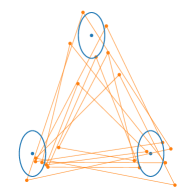
(a) $\rho=0$

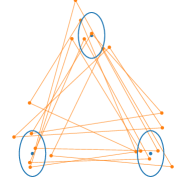
(b) $\rho=0.5$

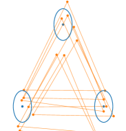
(c) $\rho=0.95$

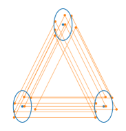
(d) $\rho=1$

Figure 2: The effect of the degree of linear correlation on the relative positions of three 2-D landmarks. The correlation is quantified using the Pearson correlation coefficient, $\rho$, for a synthetic Gaussian belief over the landmarks. Shown in blue are the marginal distributions of each landmark—the ellipses indicate the first standard deviations. Each orange triangulation of points represents a single 6-D sample from the joint distribution over all three landmarks.

Similarly, the robot pose will be highly correlated with nearby landmarks, and consequently the relative positions of the robot pose and landmarks will also be known accurately. In the ideal case, in which the robot and landmarks’ positions in the global IRF are perfectly correlated, their relative positions would be perfectly known. If we then describe $\mathit{M}$ with respect to the landmarks (that is, transforming $\mathit{M}\rightarrow\mathit{M}^{R}$), $\mathit{M}^{R}$ would be statistically independent of both the landmarks and the robot pose. This is because the relative positions of the robot and landmarks would be known perfectly, and therefore the uncertainty in the belief over $\mathit{M}^{R}$ would only stem from measurement uncertainty. Although the relative positions are never perfectly known, they are usually accurately known and it is reasonable to approximate the belief over the SLAM states and $\mathit{M}^{R}$ as statistically independent

$${\mathcal{B}}(\bm{x},\mathit{L},\mathit{M}^{R})\approx{\mathcal{B}}(\bm{x},\mathit{L}){\mathcal{B}}(\mathit{M}^{R}),$$ (7)

where

$${\mathcal{B}}(\mathit{M}^{R})\propto\prod_{i}p(\bm{z}^{R}_{i}|\bm{m}^{R}_{i}).$$ (8)

To illustrate the validity of this approximation, we visualise the absolute value of the Pearson correlation coefficient matrix for the Gaussian belief distributions ${\mathcal{B}}(\bm{x},\mathit{L},\mathit{M})$ and ${\mathcal{B}}(\bm{x},\mathit{L},\mathit{M}^{R})$ of a practical stereo vision dataset (Figures 3a and 3b). In ${\mathcal{B}}(\bm{x},\mathit{L},\mathit{M})$, we see that there is indeed a high correlation between $\bm{x}$, $\mathit{L}$ and $\mathit{M}$. Upon transforming $\mathit{M}\rightarrow\mathit{M}^{R}$, the resulting belief ${\mathcal{B}}(\bm{x},\mathit{L},\mathit{M}^{R})$ has negligible correlations between the SLAM states and $\mathit{M}^{R}$. The correlations are almost zero, which equates to SLAM states and $\mathit{M}^{R}$ being approximately statistically independent. Therefore, this process of transforming to a relative IRF decouples the process of dense mapping from the robot pose.

The main advantage of this decoupling process is highlighted in the scenario in which loop closure is performed. The belief over the environment surface points in the relative IRF is decoupled from the SLAM states; hence, when the belief over the SLAM states changes due to loop closure, the environment surface points no longer need to be reintegrated into the map—as would be required in a global IRF. Instead, the burden is placed on the SLAM algorithm to maintain (or allow the extraction of) marginal distributions over the landmarks demarcating the submaps, which is a far more tractable approach.

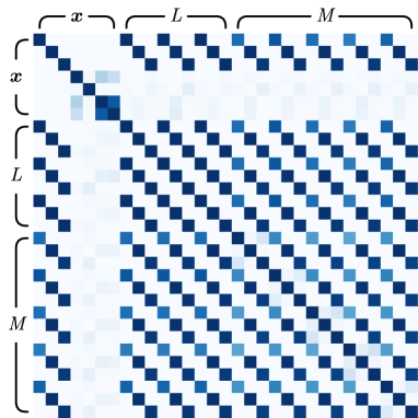
(a)

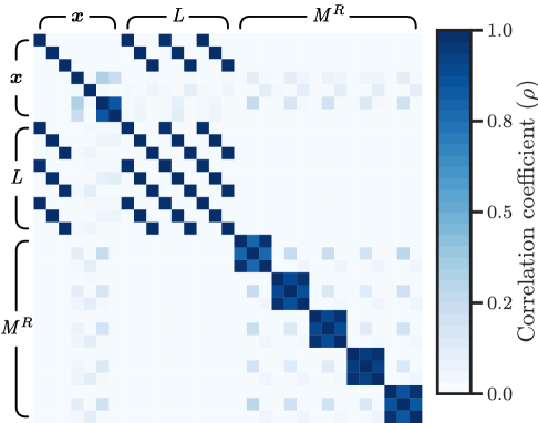
(b)

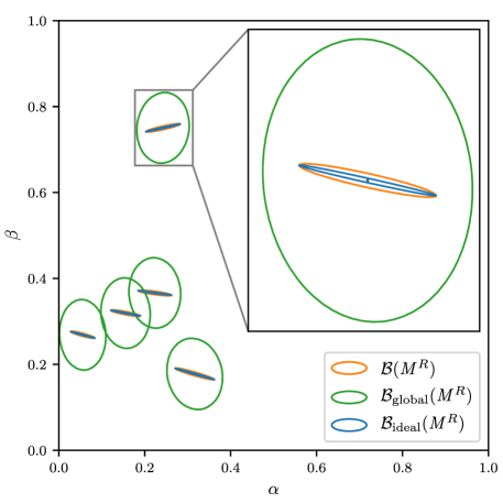
(c)

Figure 3: A visualisation of the absolute value of the Pearson correlation coefficient matrix (the darker, the more correlated) for the Gaussian belief distributions ${\mathcal{B}}(\bm{x},\mathit{L},\mathit{M})$ and (b) ${\mathcal{B}}(\bm{x},\mathit{L},\mathit{M}^{R})$. In (b) the $3\times 3$ block diagonals are from the individual 3-D environment surface points. (c) A comparison of the uncertainty in the beliefs over the environment surface measurements in a relative and global IRF. Our approximate belief, ${\mathcal{B}}(\mathit{M}^{R})$, is compared to ${\mathcal{B}}_{\text{ideal}}(\mathit{M}^{R})$ and ${\mathcal{B}}_{\text{global}}(\mathit{M}^{R})$ (see the text for further details of the belief definitions). The ellipses outline the first standard deviations of the respective belief distributions. The data in this visualisation was taken from a practical stereo vision dataset.

In order to evaluate the efficacy of performing dense mapping in a relative IRF—as opposed to a global IRF—we compare the uncertainty in the beliefs over the environment surface points in a relative and global IRF. For the case of mapping in a relative IRF, we consider our approximate belief ${\mathcal{B}}(\mathit{M}^{R})$ (Equation 8). We also consider the ideal case, in which our statistical independence approximation is exact—that is, the robot pose and landmarks are perfectly correlated or, in other words, the relative positions between $\bm{x}$ and $\mathit{L}$ are perfectly known. The uncertainty in this ideal belief, ${\mathcal{B}}_{\text{ideal}}(\mathit{M}^{R})$, is solely dependent on the measurement uncertainty. For the case of mapping in a global IRF, we consider the belief over the environment surface points in a global IRF, ${\mathcal{B}}(\mathit{M})$. To compare the beliefs in the relative IRF with that of the global IRF, we need to evaluate all the beliefs using the same units. We therefore deterministically transform ${\mathcal{B}}(\mathit{M})$ to the relative IRF using the maximum likelihood value of the landmarks; we denote the resulting belief ${\mathcal{B}}_{\text{global}}(\mathit{M}^{R})$. The resulting comparison of all the beliefs is shown in Figure 3c. From this we can conclude that the uncertainty in belief over the environment surface point used for dense mapping can be significantly less when using a relative IRF instead of a global IRF. Additionally, the uncertainty in the belief becomes almost solely dependent on the measurement uncertainty. Nieto et al. [3] noted similar effects when representing other landmarks in a relative IRF; that is, a dramatic decrease in the correlation between landmarks in the relative and global IRF, and a decrease in the marginal landmark belief uncertainty in the relative IRF.

In this section, we presented a method of decoupling the robot pose from the process of dense mapping. By transforming the information from the measured environment surface points to a relative IRF, we have approximately removed their statistical dependence on the robot pose. Next we look at incorporating this information into our model of the environment.

4 The Stochastic Triangular Mesh Map

Based on the highlighted drawbacks of the existing mapping techniques (Section 2.8), we propose a mapping technique that explicitly models the surface of the environment using STM; that is, a triangular mesh consisting of stochastic surfel, forming a continuous representation of the surface of the environment (Footnote 11).

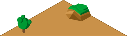
(a)

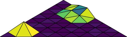
(b)

Figure 4: (a) A hypothetical environment within a triangular submap, and (b) a depiction of the corresponding *STM map. Each triangular *surfel in the mesh is coloured according to its planar deviation—the deviation of the actual surface of the environment from the triangular planes (the lighter, the higher the deviation).

Most of the existing explicit surface-mapping techniques operate under the approximation that the map can model the surface of the environment exactly. STM map, on the other hand, accounts for the fact that the surface of the environment cannot be modelled exactly with deterministic map elements; instead, the surface of the environment is treated as a stochastic process. Additionally, even if it is possible to represent the environment exactly, the representation would be very wasteful; we rather summarise the surface information relevant to the application. In contrast to most mapping techniques, STM map also captures the structure of the environment by enforcing continuity in the model. Although the principle is similar to Gaussian process mapping, we are able to update the model incrementally and in a scalable fashion.

Following the aforementioned submapping method (Section 3), we develop the STM map within a triangular submap. We partition the submap into a regular triangular grid by recursively subdividing the horizontal ($\alpha$-$\beta$) plane into equisized triangular grid elements (Figure 5). The surface of the environment within each grid element—the region normal to the grid element—is modelled by the STM map using a surfel. The submap division is performed until a desired grid element size is achieved. Depending on the application, this could be simply chosen based on the dimensions and physical capability of the robot. In general, it would be more sensible to perform this partitioning in an adaptive manner, although we do not address this in the current implementation, but will discuss this in future work (see Section 7).

Figure 5: The recursive division of a triangular submap into equisized triangular grid elements.

In the remainder of this section, we discuss how each surfel in STM map models the surface of the environment. Subsequently, we discuss performing incremental Bayesian inference on STM map (Section 5). It should also be noted that we develop the STM map within the relative IRF of a submap, and consequently, all variables are assumed to be defined in the relative IRF. However, without loss of generality, this representation could also be applied in a global IRF framework by defining the IRF accordingly, which we demonstrate in Section 6.5.

4.1 Surface Element Model

STM map consists of triangular surfel, which together form a continuous representation of the surface of the environment within the submap. We assume that the surface of the environment within the submap can be represented adequately using a 2.5-D map. At any coordinate on the horizontal plane, the environment normal to this plane need only be described using a single height. Therefore, associated with each grid element is a triangular surfel that models the surface of the environment within the grid element—the region normal to the grid element.

Figure 6: (left) The *surfel model, consisting of a mean plane—parameterised by the vertex heights $\bm{h}=\begin{bmatrix}h_{0},&h_{\alpha},&h_{\beta}\end{bmatrix}^{\intercal}$—and a planar deviation $\nu$. (right) A 2-D slice of the surfel (orange) of an underlying surface (green). The shaded region indicates the one standard deviation confidence interval. $\mathcal{N}_{m}(\cdot)$ denotes the moment form of a Gaussian distribution.

If we initially consider a map with a single grid element, the maximum length along both the $\alpha$- and $\beta$-axes within the grid element will be unity—Equation 2. The associated surfel models the surface of the environment within the grid element as a stochastic process—a mean plane and a homoscedastic deviation from it, normal to the grid element (Figure 6). This simple model does not try to exactly represent the actual surface of the environment, but summarises the key aspects of the surface instead. This is an efficient representation for the purpose of robotic navigation, since the model captures the relevant aspects of the environment, and avoids modelling unnecessary details that are not relevant for the intended application. We consider this to be an advantage rather than a disadvantage. More precisely, a point on the surface of the environment at some given coordinates $(\alpha,\beta)$ is modelled by the stochastic process

$$\begin{split}\gamma&=f(\alpha,\beta,\bm{h})+\epsilon\\ &=\begin{bmatrix}1-\alpha-\beta&\alpha&\beta\end{bmatrix}\bm{h}+\epsilon,\end{split}$$ (9)

where $f(\alpha,\beta,\bm{h})$ describes a point on the mean plane, and $\epsilon\sim\mathcal{N}_{m}(\epsilon;0,\nu)$ models the deviation of the actual surface from the mean plane. We refer to the variance of the stochastic process, $\nu$, as the planar deviation. The mean plane is specified using the normal heights at each of the vertices of the grid element

$$\bm{h}=\begin{bmatrix}[c]h_{0}\\ h_{\alpha}\\ h_{\beta}\end{bmatrix},$$ (10)

where $h_{0}$, $h_{\alpha}$, and $h_{\beta}$ are the heights at $(\alpha,\beta)=(0,0)$, $(1,0)$ and $(0,1)$ respectively. Consequently, the surfel model is parameterised by $\bm{h}$ and $\nu$, which we combine into a single parameter vector, $\bm{\theta}=\begin{bmatrix}\bm{h}&\nu\end{bmatrix}^{\intercal}$. This simple stochastic process allows us to account for a wide range of surfaces by essentially summarising the underlying environment within the grid element. It should be noted that we follow a Bayesian modelling approach, treating the map parameters as random variables. We specifically model the surfels’ heights as Gaussian distributed, and the planar deviation as inverse-gamma distributed. We expand on this when discussing performing inference on the model (Section 5).

In order to generalise this definition of the surfel model from a single to multiple grid elements within a submap, we normalise each grid element—scaling the maximum length of the $\alpha$- and $\beta$-axes to unity, and shifting to the origin. This normalisation does not affect the values of the surfel parameters, $\bm{\theta}$, which are defined with respect to the $\gamma$-axis. Additionally, as this is a deterministic linear operation, the Gaussian measurement distributions in this normalised grid element remain exactly Gaussian distributed, which will be important when performing inference on the surfel model parameters (Section 5).

To create a continuous representation, the mean planes of surfels in contiguous grid elements are constrained to be continuous; that is, the heights at their shared vertices should be equal (Figure 7). However, we do not enforce any constraints on the planar deviations between surfels. The continuous surface in a submap formed by the mean plane in each surfel describes the mean mesh, which is parameterised by the ordered set of unique vertex heights, $\mathit{H}$. The stochastic deviation from this mean mesh is parameterised by the ordered set of planar deviations in each surfel, $\mathit{V}$. Both $\mathit{H}$ and $\mathit{V}$ fully parameterise STM map, which can be combined into a single ordered set, $\mathit{\Theta}$.

(a)

(b)

Figure 7: STM forms a continuous representation of the surface of the environment. We visualise (a) the mean mesh, and (b) a slice through the STM map (orange) of an underlying surface (green). The shaded region indicates the one standard deviation confidence interval in the respective surfels.

We have defined how the constituent surfels of STM map model the environment; we now seek to determine the parameter values for STM map based on measurements of the surface of the environment—in other words, to perform inference.

5 Model Inference

Based on the definition of STM map, we now wish to infer the values of the map parameters, $\mathit{\Theta}$, for some given noisy measurements of the surface of the environment, $\mathit{Z}=\mathtt{Z}$. We follow a Bayesian modelling approach, maintaining a belief distribution over the map parameters. We would therefore ideally like to calculate the joint belief distribution over all the map parameters

$${\mathcal{B}}(\mathit{\Theta})=p(\mathit{\Theta}|\mathit{Z}=\mathtt{Z}).$$ (11)

However, for large maps, this would quickly become intractable to store, as the storage grows quadratically with the number of surfels in the map (for our choice of continuous parametric distributions). To circumvent this issue, we instead directly calculate the marginal belief for each surfel’s parameters

$${\mathcal{B}}(\bm{\theta})=p(\bm{\theta}|\mathit{Z}=\mathtt{Z}),$$ (12)

for which storage grows linearly with each added surfel.

Next we will look at calculating each surfel’s belief independently of the rest of the map (Section 5.1); this is equivalent to neglecting the continuity constraints between surfels. Building upon this, we expand to performing inference on the full model (Section 5.2). Finally, we summarise the inference algorithm for STM map, and discuss the implementation thereof (Section 5.3).

5.1 Single Surfel Inference

We initially consider each surfel in isolation, and wish to calculate the belief distribution over a single surfel’s parameters, $\bm{\theta}=\begin{bmatrix}\bm{h}&\nu\end{bmatrix}^{\intercal}$, from noisy measurements associated with the respective grid element. We combine this approach to handle multiple surfels in Section 5.2, but it is useful to first consider this perspective before performing inference on the full model.

Most probabilistic problems involve several random variables; PGM provide a compact graphical representation over this complex high-dimensional space, which is useful in both modelling and performing inference. There are many different PGMs for different types of problems (or questions); in our case we focus on three types of PGMs: Bayesian networks, factor graphs, and cluster graphs. A Bayesian network, or belief network, represents the conditional independence assumptions in the joint distribution as a directed graph between random variable nodes. The Bayesian network representation of the surfel model we use is shown in Figure 8a, which equivalently represents the factorisation over the joint distribution

$$\begin{split}&p(\bm{\theta},\mathit{M},\mathit{Z}=\mathtt{Z})=p(\bm{\theta})\underbrace{\prod_{i}p(\bm{z}_{i}=\mathtt{z}_{i}|\bm{m}_{i})\,\overbrace{p(\gamma_{i}|\alpha_{i},\beta_{i},\bm{\theta})\,p(\alpha_{i})\,p(\beta_{i})}^{p(\bm{m}_{i}|\bm{\theta})}}_{p(\mathit{M},\mathit{Z}=\mathtt{Z}|\bm{\theta})},\end{split}$$ (13)

where $\mathit{Z}=(\bm{z}_{i})$ is the sequence of noisy measurements corresponding to the points on the surface of the environment, $\mathit{M}=(\bm{m}_{i})$, as mentioned in Section 3.2. This factorisation of the joint distribution models the generative process of measurements—the model parameters describe where actual points on the surface in the environment lie, and these points are observed through measurements of the environment. In the measurement mode, $p(\bm{z}_{i}=\mathtt{z}_{i}|\bm{m}_{i})$, we assume that a measurement, $\bm{z}_{i}$, is only dependent on the corresponding point on the actual surface of the environment, $\bm{m}_{i}$; this measurement distribution was derived in Section 3.2. In $p(\gamma_{i}|\alpha_{i},\beta_{i},\bm{\theta})$, we assume that the height of the surface point, $\gamma_{i}$, is only dependent on the grid element coordinates $(\alpha_{i},\beta_{i})$ and the surfel parameters, $\bm{\theta}$. This is based on the definition of the stochastic process in the surfel model—Equation 9.

From this Bayesian network we can construct a factor graph (Figure 8b). It represents the fully factorised functional form of the joint distribution in an undirected graph, where the random variables are linked by the factors they share. These factors can be grouped into clusters, resulting in a cluster graph representation (Figure 8c). The combined factors in a cluster are known as the cluster potential, and shared links between clusters are defined by their sepset—a subset of the shared variables. Although there is a unique factor graph for a Bayesian network, the grouping of factors in a cluster graph is, in general, non-unique. We choose to group all the factors inside the plate into a cluster, and the factor outside the plate into a cluster. Both factor and cluster graphs can be used for inference, although we will focus on inference in cluster graphs.

(a) Bayesian network

(b) Factor graph

(c) Cluster graph

Figure 8: Different types of probabilistic graphical models representing the inference problem for our surfel model. The surfel model parameters, $\bm{\theta}=\begin{bmatrix}\bm{h}&\nu\end{bmatrix}^{\intercal}$, measurements, $\bm{z}_{i}$, and corresponding points on the surface of the environment, $\bm{m}_{i}=\begin{bmatrix}\alpha_{i}&\beta_{i}&\gamma_{i}\end{bmatrix}^{\intercal}$, are all random variables. We use plate notation, where the solid rectangular plates indicate a repetition of the subgraph therein. (a) The dotted rectangle denotes an expanded vector, and the shaded circle indicates an observed (or given) variable. (b) Factors are indicated with $\blacksquare$. (c) Cluster potentials and messages are denoted $\phi(\cdot)$ and $\delta(\cdot)$ respectively, and the sepset between clusters is indicated with $\boxdot$.

As a cluster graph is the result of grouping factors from the joint distribution, we can equivalently represent the joint distribution as the product over all the cluster potentials

$$p(\bm{\theta},\mathit{M},\mathit{Z}=\mathtt{Z})=\phi_{p}(\bm{\theta})\prod_{i}\phi_{i}(\bm{\theta},\bm{m}_{i}),$$ (14)

where we refer to $\phi_{p}(\bm{\theta})$ as the prior cluster potential and each $\phi_{i}(\bm{\theta},\bm{m}_{i})$ as a likelihood cluster potential. We wish to infer the surfel belief distribution for some given measurements, $\mathit{Z}=\mathtt{Z}$. Using Bayes’ theorem, we can express this belief in terms of the joint distribution

$$\begin{split}{\mathcal{B}}(\bm{\theta})&=p(\bm{\theta}|\mathit{Z}=\mathtt{Z})\\ &\propto\int\displaylimits_{\mathit{M}}p(\bm{\theta},\mathit{M},\mathit{Z}=\mathtt{Z})\,\text{d}\mathit{M}\\ &\propto\phi_{p}(\bm{\theta})\prod_{i}\int\displaylimits_{\bm{m}_{i}}\phi_{i}(\bm{\theta},\bm{m}_{i})\,\text{d}\bm{m}_{i}.\end{split}$$ (15)

An equivalent method of calculating this belief is by using message passing. For inference in cluster graphs, the outgoing and incoming messages for each cluster needs to be calculated. According to the integral-product algorithm, the outgoing message from the $i$-th likelihood cluster is defined as

$$\delta{{}_{i\shortrightarrow p}}(\bm{\theta})=\int\displaylimits_{\bm{m}_{i}}\phi_{i}(\bm{\theta},\bm{m}_{i})\,\text{d}\bm{m}_{i}.$$ (16)

Similarly, the incoming message to the $i$-th likelihood cluster is defined as

$$\begin{split}\delta{{}_{i\shortleftarrow p}}(\bm{\theta})&=\phi_{p}(\bm{\theta})\prod_{j\neq i}\delta{{}_{j\shortrightarrow p}}(\bm{\theta}).\end{split}$$ (17)

By comparing Equation 15 with Equations 16 and 17, we can see that the product of these messages equivalently specifies the surfel belief

$${\mathcal{B}}(\bm{\theta})\propto\delta{{}_{i\shortrightarrow p}}(\bm{\theta})\delta{{}_{i\shortleftarrow p}}(\bm{\theta}).$$ (18)

However, there is no convenient closed-form solution to either of the messages—and consequently the surfel belief. This is due to nonlinear relationships between the random variables in the likelihood cluster potentials. In order to find a tractable solution to the surfel belief, we have to perform approximate inference. We specifically focus on variational inference, which projects a desired (intractable) probability distribution onto an approximating family of distributions. This projection is performed by minimising a chosen information divergence—a measure of similarity—between the exact and approximate distributions. A commonly-used information divergence is the KL divergence

$$D_{\text{KL}}\left(q(x)\,\middle\|\,p(x)\right)\triangleq\int\displaylimits_{x}q(x)\log\frac{q(x)}{p(x)}\,dx,$$ (19)

which is a positive measure of relative entropy between two probability distributions $p(x)$ and $q(x)$. We minimise the exclusive KL divergence to calculate an approximate surfel belief

$$\tilde{\mathcal{B}}(\bm{\theta})=\operatorname*{arg\,min}_{\tilde{\mathcal{B}}(\bm{\theta})\in\mathcal{F}}D_{\text{KL}}\left(\tilde{\mathcal{B}}(\bm{\theta})\,\middle\|\,{\mathcal{B}}(\bm{\theta})\right),$$ (20)

where $\mathcal{F}$ is a family of approximating distributions. This process of minimising the exclusive KL divergence is commonly referred to as the information projection; alternatively minimising the inclusive KL divergence is referred to as the moment projection. As opposed to minimising this global divergence, a group of techniques known as approximate message passing distributes the problem of variational inference by instead incrementally performing local projections with the aim of approximately minimising the global divergence. In essence, message passing minimises the global divergence using coordinate descent. This can be explained intuitively in the context of performing inference in a cluster graph. Message passing iteratively approximates each cluster potential; at each iteration, a certain cluster potential is approximated, while keeping all other cluster potentials constant. The constant cluster potentials determine the incoming message of the cluster potential being approximated, and are used as context to update the approximation (how the approximation is updated depends on the chosen divergence measure). This process is repeated until convergence, upon which the global divergence is assumed to be at a (local) minimum.

Performing message passing for our chosen divergence measure is known as VMP [55]. If we were to instead minimise the inclusive KL divergence (moment projection), this would result in the EP message passing technique [56]. A notable property of VMP is that a fixed point in performing message passing is also a stationary point in the global divergence—in other words, minimising local divergences is equivalent to minimising the global divergence. VMP is also the only message passing technique with this property, whereas other message passing techniques only approximate it [54]; this is as a result of VMP using the exclusive KL divergence.

In order to calculate the approximate surfel belief,

$$\tilde{\mathcal{B}}(\bm{\theta})\propto\tilde{\delta}{{}_{i\shortrightarrow p}}(\bm{\theta})\tilde{\delta}{{}_{i\shortleftarrow p}}(\bm{\theta}),$$ (21)

the approximate messages, $\tilde{\delta}{{}_{i\shortrightarrow p}}(\bm{\theta})$ and $\tilde{\delta}{{}_{i\shortleftarrow p}}(\bm{\theta})$, are calculated by replacing $\phi_{i}(\bm{\theta},\bm{m}_{i})$ by an approximating likelihood cluster potential, $\tilde{\phi}_{i}(\bm{\theta},\bm{m}_{i})$, in Equations 17 and 16. To calculate each approximate likelihood cluster potential, VMP performs a local information projection

$$\tilde{\phi}_{i}(\bm{\theta},\bm{m}_{i})=\operatorname*{arg\,min}_{\tilde{\phi}_{i}\in\mathcal{F}}D_{\text{KL}}\left(\tilde{\phi}_{i}\tilde{\delta}{{}_{i\shortleftarrow p}}\,\middle\|\,\phi_{i}\tilde{\delta}{{}_{i\shortleftarrow p}}\right),$$ (22)

where $\mathcal{F}$ is a family of approximating distributions (we omit the arguments of the functions to declutter the notation). It should be noted that this is an iterative process, as we must perform this local projection for each likelihood cluster potential. To make this local projection tractable, we also make the simplifying assumption that each approximating likelihood cluster potential is of the factorised form

$$\tilde{\phi}_{i}(\bm{\theta},\bm{m}_{i})=\tilde{\phi}_{i}(\bm{h},\bm{m}_{i})\tilde{\phi}_{i}(\nu).$$ (23)

This factorisation over disjoint sets of the random variables is a commonly-used approximation referred as the structured mean-field approximation [57]. We choose this structured factorisation in particular, as it more accurately represents the exact distribution compared to a full factorisation. In contrast to other structured factorisation combinations, it groups variables from the same distribution family (as we will soon show). We also assume the prior cluster potential to be of a similar factorised form,

$$\phi_{p}(\bm{\theta})=\phi_{p}(\bm{h})\phi_{p}(\nu),$$ (24)

therefore the approximate messages and surfel belief will be similarly factorised.

In order to perform the minimisation in Equation 22, we first need to specify the family of approximating distributions for the factors of $\tilde{\phi}_{i}(\bm{\theta},\bm{m}_{i})$. For the factor over $\bm{h}$ and $\bm{m}_{i}$, we choose the Gaussian distribution

$$\tilde{\phi}_{i}(\bm{h},\bm{m}_{i})=\mathcal{N}_{c}(\begin{bmatrix}\bm{h}&\bm{m}_{i}\end{bmatrix}^{\intercal};\bm{\xi}_{i},\bm{\Omega}_{i}),$$ (25)

where $\bm{\xi}_{i}$ is the information vector and $\bm{\Omega}_{i}$ is the information matrix of the Gaussian distribution in canonical form. For the factor over $\nu$, we choose the inverse-gamma distribution

$$\tilde{\phi}_{i}(\nu)=\Gamma^{-1}(\nu;a_{i},b_{i}),$$ (26)

where $a_{i}$ is the shape parameter and $b_{i}$ the scale parameter of the inverse-gamma distribution. The resulting product of these distributions—Equation 23—should not be confused with a normal-inverse-gamma distribution. In our case, this is simply the product of these two distributions without any conditional dependencies.

If we had already calculated the approximate likelihood cluster potential, $\tilde{\phi}_{i}(\bm{\theta},\bm{m}_{i})$, we could calculate the outgoing message using Equation 16, which would result in the distribution

$$\tilde{\delta}{{}_{i\shortrightarrow p}}(\bm{\theta})=\underbrace{\mathcal{N}_{c}(\bm{h};\bm{\xi}_{i\shortrightarrow p},\bm{\Omega}_{i\shortrightarrow p})}_{\tilde{\delta}{{}_{i\shortrightarrow p}}(\bm{h})}\underbrace{\Gamma^{-1}(\nu;a_{i\shortrightarrow p}-1,b_{i\shortrightarrow p})}_{\tilde{\delta}{{}_{i\shortrightarrow p}}(\nu)}.$$ (27)

We assume that the prior cluster potential is also similarly distributed, as

$$\begin{split}\phi_{p}(\bm{\theta})&=\underbrace{\mathcal{N}_{c}(\bm{h};\bm{\xi}_{p},\bm{\Omega}_{p})}_{\phi_{p}(\bm{h})}\underbrace{\Gamma^{-1}(\nu;a_{p},b_{p})}_{\phi_{p}(\nu)}.\end{split}$$ (28)

Both the Gaussian and inverse-gamma families of distributions are part of the exponential family [58]. These have the convenient property that the product and division of distributions in the family also results in a distribution in the family [54] (up to a proportionality constant), which amounts to the addition and subtraction of their natural parameters respectively. We therefore can calculate the approximate incoming message to a cluster, which will be distributed similarly to its constituents,

$$\tilde{\delta}{{}_{i\shortleftarrow p}}(\bm{\theta})=\underbrace{\mathcal{N}_{c}(\bm{h};\bm{\xi}_{i\shortleftarrow p},\bm{\Omega}_{i\shortleftarrow p})}_{\tilde{\delta}{{}_{i\shortleftarrow p}}(\bm{h})}\underbrace{\Gamma^{-1}(\nu;a_{i\shortleftarrow p},b_{i\shortleftarrow p})}_{\tilde{\delta}{{}_{i\shortleftarrow p}}(\nu)}.$$ (29)

According to Equation 17, the natural parameters of $\tilde{\delta}{{}_{i\shortleftarrow p}}(\bm{h})$ are calculated as

$$\bm{\Omega}_{i\shortleftarrow p}=\bm{\Omega}_{p}+\sum_{j\neq i}\bm{\Omega}_{j\shortrightarrow p}\;\text{ and }\;\bm{\xi}_{i\shortleftarrow p}=\bm{\xi}_{p}+\sum_{j\neq i}\bm{\xi}_{j\shortrightarrow p},$$ (30)

and the natural parameters of $\tilde{\delta}{{}_{i\shortleftarrow p}}(\nu)$ are calculated as

$$a_{i\shortleftarrow p}=a_{p}+\sum_{j\neq i}a_{j\shortrightarrow p}\;\text{ and }\;b_{i\shortleftarrow p}=b_{p}+\sum_{j\neq i}b_{j\shortrightarrow p}.$$ (31)

The same is true for the approximate surfel belief,

$$\begin{split}\tilde{\mathcal{B}}(\bm{\theta})&=\underbrace{\mathcal{N}_{c}(\bm{h};\bm{\xi}_{h},\bm{\Omega}_{h})}_{\tilde{\mathcal{B}}(\bm{h})}\underbrace{\Gamma^{-1}(\nu;a_{\nu},b_{\nu})}_{\tilde{\mathcal{B}}(\nu)}.\end{split}$$ (32)

According to Equation 21, the natural parameters of $\tilde{\mathcal{B}}(\bm{h})$ are calculated as

$$\bm{\Omega}_{h}=\bm{\Omega}_{i\shortrightarrow p}+\bm{\Omega}_{i\shortleftarrow p}\;\text{ and }\;\bm{\xi}_{h}=\bm{\xi}_{i\shortrightarrow p}+\bm{\xi}_{i\shortleftarrow p},$$ (33)

and the natural parameters of $\tilde{\mathcal{B}}(\nu)$ are calculated as

$$a_{\nu}=a_{i\shortrightarrow p}+a_{i\shortleftarrow p}\;\text{ and }\;b_{\nu}=b_{i\shortrightarrow p}+b_{i\shortleftarrow p}.$$ (34)

Performing VMP with the structured mean-field approximation therefore allows us to perform tractable inference to obtain an approximation of the surfel belief. Up to this point, we have assumed that we have the approximate likelihood cluster potentials, $\tilde{\phi}_{i}(\bm{\theta},\bm{m}_{i})$. We now discuss exactly how to calculate each of the factors of approximate likelihood cluster potentials and, consequently, the outgoing message, $\tilde{\delta}{{}_{i\shortrightarrow p}}(\bm{\theta})$.

5.1.1 Updating $\tilde{\phi}_{i}(\bm{h},\bm{m}_{i})$

The iterative update of $\tilde{\phi}_{i}(\bm{h},\bm{m}_{i})$ that would perform the local information projection of Equation 22 can be calculated according to the VMP algorithm [55] as

$$\begin{split}&\log\tilde{\phi}_{i}(\bm{h},\bm{m}_{i})+\log\tilde{\delta}{{}_{i\shortleftarrow p}}(\bm{h})\\ &\propto\left\langle\log\phi_{i}(\bm{\theta},\bm{m}_{i},\bm{z}_{i}=\mathtt{z}_{i})\tilde{\delta}{{}_{i\shortleftarrow p}}(\bm{\theta})\right\rangle_{\tilde{\mathcal{B}}(\nu)},\end{split}$$ (35)

where $\langle{\cdot}\rangle$ denotes the expectation operation. In order to arrive at a solution to $\tilde{\phi}_{i}(\bm{h},\bm{m}_{i})$, it is convenient to first describe the process of calculating the approximate belief,

$$\tilde{\mathcal{B}}(\bm{h},\bm{m}_{i})\propto\tilde{\phi}_{i}(\bm{h},\bm{m}_{i})\tilde{\delta}{{}_{i\shortleftarrow p}}(\bm{h}),$$ (36)

and then to divide out the message $\tilde{\delta}{{}_{i\shortleftarrow p}}(\bm{h})$ to recover the desired approximate to the cluster potential $\tilde{\phi}_{i}(\bm{h},\bm{m}_{i})$. Rearranging Equation 35 in terms of $\tilde{\mathcal{B}}(\bm{h},\bm{m}_{i})$ we can calculate the expectation

$$\begin{split}\log\tilde{\mathcal{B}}(\bm{h},\bm{m}_{i})&\propto\left\langle\log\left(\phi_{i}(\bm{\theta},\bm{m}_{i})\tilde{\delta}{{}_{i\shortleftarrow p}}(\bm{\theta})\right)\right\rangle_{\tilde{\mathcal{B}}(\nu)}\\ &\begin{split}=&\log p(\gamma_{i}|\alpha_{i},\beta_{i},\bm{h},\nu=\nu_{{\mathcal{B}}})\\ &+\log p(\bm{z}_{i}=\mathtt{z}_{i}|\bm{m}_{i})\\ &+\log\left(p(\alpha_{i})p(\beta_{i})\tilde{\delta}{{}_{i\shortleftarrow p}}(\bm{h})\right),\end{split}\end{split}$$ (37)

where

$$\nu_{{\mathcal{B}}}=\left\langle\nu^{-1}\right\rangle_{\tilde{\mathcal{B}}(\nu)}^{-1}=\frac{b_{\nu}}{a_{\nu}}.$$ (38)

In order to find an analytical expression for $\tilde{\mathcal{B}}(\bm{h},\bm{m}_{i})$, we consider each of the constituent distributions in Equation 37. As mentioned in Section 3.2, the measurement distribution is Gaussian distributed, which can be rearranged such that the mean of the distribution is the observation

$$\begin{split}p(\bm{z}_{i}=\mathtt{z}_{i}|\bm{m}_{i})&=\mathcal{N}_{m}(\bm{z}_{i}=\mathtt{z}_{i};\bm{m}_{i},\bm{\Sigma}_{z_{i}})\\ &=\mathcal{N}_{m}(\bm{m}_{i};\mathtt{z}_{i},\bm{\Sigma}_{z_{i}}).\end{split}$$ (39)

According to the surfel model in Section 4, the likelihood distribution is Gaussian distributed

$$p(\gamma_{i}|\alpha_{i},\beta_{i},\bm{h},\nu_{{\mathcal{B}}})=\mathcal{N}_{m}(\gamma_{i};f(\bm{h},\alpha_{i},\beta_{i}),\nu_{{\mathcal{B}}}),$$ (40)

where $f(\cdot)$ is the mean of the stochastic process as defined in Equation 9. We place an uninformative and independently distributed Gaussian prior over $\alpha_{i}$ and $\beta_{i}$, and combine it with $\tilde{\delta}{{}_{i\shortleftarrow p}}(\bm{h})$ to form the jointly Gaussian distributed context distribution

$$p(\alpha_{i})p(\beta_{i})\tilde{\delta}{{}_{i\shortleftarrow p}}(\bm{h})=\mathcal{N}_{m}(\begin{bmatrix}\bm{h}&\alpha_{i}&\beta_{i}\end{bmatrix}^{\intercal};\bm{\mu}_{c},\bm{\Sigma}_{c}),$$ (41)

with moments calculated as

$$\bm{\mu}_{c}=\begin{bmatrix}\bm{\mu}_{i\shortleftarrow p}\\ \mu_{\alpha_{i}}\\ \mu_{\beta_{i}}\end{bmatrix}\;\text{ and }\;\bm{\Sigma}_{c}=\operatorname*{diag}(\bm{\Sigma}_{i\shortleftarrow p},\sigma^{2}_{\alpha_{i}},\sigma^{2}_{\beta_{i}}),$$ (42)

where $\bm{\Sigma}_{i\shortleftarrow p}=\bm{\Omega}_{i\shortleftarrow p}^{-1}$, $\bm{\mu}_{i\shortleftarrow p}=\bm{\Sigma}_{i\shortleftarrow p}\bm{\xi}_{i\shortleftarrow p}$, and the $\operatorname*{diag}(\cdot)$ operator creates a block diagonal matrix of its arguments. Most notably, all distributions except the likelihood distribution are exactly Gaussian distributed over $\bm{h}$ and $\bm{m}_{i}$. This dissimilarity in likelihood distribution is due to the nonlinear relationships introduced by $f(\cdot)$. To ensure that the product of all the distributions is tractable, we also wish to approximate the likelihood distribution as a Gaussian distribution. A common approach to achieving this is by linearising; we therefore use a linear Taylor series approximation,

$$f(\bm{x})\approx f(\bar{\bm{x}})+\bm{F}(\bm{x}-\bar{\bm{x}}),$$ (43)

where $\bm{x}=\begin{bmatrix}\bm{h}&\alpha_{i}&\beta_{i}\end{bmatrix}^{\intercal}$, and $\bm{F}$ is the Jacobian matrix of $f(\bm{x})$ evaluated at the linearisation point $\bm{\mu}_{c}$:

$$\begin{split}\bm{F}&=\left.\frac{\delta f}{\delta\bm{x}}\right|_{\bm{x}=\bm{\mu}_{c}}=\left.\begin{bmatrix}1-\alpha_{i}-\beta_{i}&\alpha_{i}&\beta_{i}&h_{\alpha}-h_{0}&h_{\beta}-h_{0}\end{bmatrix}\right|_{\bm{\mu}_{c}}\end{split}.$$ (44)

Using this we can calculate the product of the likelihood and context distributions,

$$\begin{split}&p(\gamma_{i}|\alpha_{i},\beta_{i},\bm{h},\nu_{{\mathcal{B}}})p(\alpha_{i})p(\beta_{i})\tilde{\delta}{{}_{i\shortleftarrow p}}(\bm{h})\\ &\propto\mathcal{N}_{c}(\begin{bmatrix}\bm{h}&\bm{m}_{i}\end{bmatrix}^{\intercal};\bar{\bm{\xi}},\bar{\bm{\Omega}})\end{split},$$ (45)

with natural parameters calculated as

$$\begin{split}\bar{\bm{\xi}}&=\bar{\bm{\Omega}}\begin{bmatrix}\bm{\mu}_{c}\\ f(\bm{\mu}_{c})\end{bmatrix}\end{split}\;\text{ and }\;\begin{split}\bar{\bm{\Omega}}&=\begin{bmatrix}\bm{\Sigma}_{c}&(\bm{F}\bm{\Sigma}_{c})^{\intercal}\\ \bm{F}\bm{\Sigma}_{c}&\bm{F}\bm{\Sigma}_{c}\bm{F}^{\intercal}+\nu_{{\mathcal{B}}}\\ \end{bmatrix}^{-1}.\end{split}$$ (46)

The normalised product of the prediction distribution and the measurement distribution results in the desired belief

$$\tilde{\mathcal{B}}(\bm{h},\bm{m}_{i})=\mathcal{N}_{c}(\begin{bmatrix}\bm{h}&\bm{m}_{i}\end{bmatrix}^{\intercal};\bm{\xi},\bm{\Omega}),$$ (47)

with natural parameters calculated as

$$\begin{split}\bm{\xi}&=\bar{\bm{\xi}}+\bm{S}^{\intercal}\bm{\Sigma}_{z_{i}}^{-1}\mathtt{z}_{i}\\ &=\begin{bmatrix}\bm{\xi}_{h}\\ \bm{\xi}_{m}\end{bmatrix}\end{split}\quad\text{ and }\quad\begin{split}\bm{\Omega}&=\bar{\bm{\Omega}}+\bm{S}^{\intercal}\bm{\Sigma}_{z_{i}}^{-1}\bm{S}\\ &=\begin{bmatrix}\bm{\Omega}_{hh}&\bm{\Omega}_{hm}\\ \bm{\Omega}_{mh}&\bm{\Omega}_{mm}\\ \end{bmatrix}\end{split},$$ (48)

where $\bm{S}=\begin{bmatrix}\bm{0}_{3\text{x}3}&\bm{I}_{3\text{x}3}\end{bmatrix}$ is a selection matrix. Notably, the above method is equivalent to an extended information filter (EIF) with a nonlinear state transition model and a linear measurement model [59, ch. 3.5.4]. Finally, we can calculate $\tilde{\phi}_{i}(\bm{h},\bm{m}_{i})$ by dividing out $\tilde{\delta}{{}_{i\shortleftarrow p}}(\bm{h})$ from $\tilde{\mathcal{B}}(\bm{h},\bm{m}_{i})$ (Equation 36), which results in

$$\tilde{\phi}_{i}(\bm{h},\bm{m}_{i})=\mathcal{N}_{c}(\begin{bmatrix}\bm{h}&\bm{m}_{i}\end{bmatrix}^{\intercal};\bm{\xi}_{i},\bm{\Omega}_{i}),$$ (49)

with natural parameters calculated as

$$\begin{split}\bm{\xi}_{i}&=\begin{bmatrix}\bm{\xi}_{h}-\bm{\xi}_{i\shortleftarrow p}\\ \bm{\xi}_{m}\end{bmatrix}\end{split}\;\text{ and }\;\begin{split}\bm{\Omega}_{i}&=\begin{bmatrix}\bm{\Omega}_{hh}-\bm{\Omega}_{i\shortleftarrow p}&\bm{\Omega}_{hm}\\ \bm{\Omega}_{mh}&\bm{\Omega}_{mm}\\ \end{bmatrix}.\end{split}$$ (50)

From this result, we can now calculate a part of the outgoing message, $\tilde{\delta}{{}_{i\shortrightarrow p}}(\bm{h})$, by marginalising out $\bm{m}_{i}$. Therefore, using Equation 16, we can calculate the natural parameters of $\tilde{\delta}{{}_{i\shortrightarrow p}}(\bm{h})$ (Equation 27) as

$$\begin{split}\bm{\Omega}_{i\shortrightarrow p}&=\bm{\Omega}_{hh}-\bm{\Omega}_{j\shortleftarrow p}-\bm{\Omega}_{hm}\bm{\Omega}_{mm}^{-1}\bm{\Omega}_{mh}\end{split}$$ (51)

and

$$\begin{split}\bm{\xi}_{i\shortrightarrow p}&=\bm{\xi}_{h}-\bm{\xi}_{j\shortleftarrow p}-\bm{\Omega}_{hm}\bm{\Omega}_{mm}^{-1}\bm{\xi}_{m}.\end{split}$$ (52)

We have now discussed how to calculate the likelihood cluster potential $\tilde{\phi}_{i}(\bm{h},\bm{m}_{i})$ and the outgoing message $\tilde{\delta}{{}_{i\shortrightarrow p}}(\bm{h})$. Next, we focus on the likelihood cluster potential and outgoing message over the planar deviation.

5.1.2 Updating $\tilde{\phi}_{i}(\nu)$

Similarly to calculating $\tilde{\phi}_{i}(\bm{h},\bm{m}_{i})$, to perform the local information projection of Equation 22 with respect to $\tilde{\phi}_{i}(\nu)$, the VMP algorithm [55] defines the iterative update as

$$\begin{split}&\log\tilde{\phi}_{i}(\nu)+\log\tilde{\delta}{{}_{i\shortleftarrow p}}(\nu)\propto\left\langle\log\phi_{i}(\bm{\theta},\bm{m}_{i})\tilde{\delta}{{}_{i\shortleftarrow p}}(\bm{\theta})\right\rangle_{\tilde{\mathcal{B}}(\bm{h},\bm{m}_{i})}.\end{split}$$ (53)

The marginalisation to calculate the outgoing message, $\tilde{\delta}{{}_{i\shortrightarrow p}}(\bm{\theta})$—Equation 16—will have no effect on the outgoing message, $\tilde{\delta}{{}_{i\shortrightarrow p}}(\nu)$, due to our choice of factorisation. Therefore, solving for the cluster potential is equivalent to solving for the outgoing message—$\tilde{\delta}{{}_{i\shortrightarrow p}}(\nu)=\tilde{\phi}_{i}(\nu)$—which we can directly calculate as

$$\begin{split}\log\tilde{\delta}{{}_{i\shortrightarrow p}}(\nu)&\propto\left\langle\log p(\gamma_{i}|\alpha_{i},\beta_{i},\bm{h},\nu)\right\rangle_{\tilde{\mathcal{B}}(\bm{h},\bm{m}_{i})}\\ &\propto-a_{i\shortrightarrow p}\log\nu-\frac{b_{i\shortrightarrow p}}{\nu},\end{split}$$ (54)

where $\tilde{\mathcal{B}}(\bm{h},\bm{m}_{i})$ is calculated from Equation 37. The resulting approximate potential matches the form of an inverse-gamma distribution, with shape and scale parameters

$$a_{i\shortrightarrow p}=\frac{1}{2}\;\;\text{ and }\;\;b_{i\shortrightarrow p}=\frac{1}{2}\left\langle(\gamma_{i}-f(\alpha_{i},\beta_{i},\bm{h}))^{2}\right\rangle_{\tilde{\mathcal{B}}(\bm{h},\bm{m}_{i})},$$ (55)

where $f(\cdot)$ is defined by Equation 9. We again use the linear Taylor series approximation to calculate the expectation, where we linearise around the mean of $\tilde{\mathcal{B}}(\bm{h},\bm{m}_{i})$. This results in the expectation

$$b_{i\shortrightarrow p}=\frac{1}{2}\bm{F}_{\text{aug}}\bm{\Sigma}\bm{F}_{\text{aug}}^{\intercal}+\frac{1}{2}(\mu_{\gamma}-f(\mu_{\alpha},\mu_{\beta},\bm{\mu}_{h}))^{2},$$ (56)

where $\bm{F}_{\text{aug}}=\begin{bmatrix}\bm{F}&1\end{bmatrix}$—with $\bm{F}$ defined by Equation 44—and $\bm{\Sigma}=\bm{\Omega}^{-1}$ and $\bm{\mu}=\bm{\Sigma}\bm{\xi}$ are the moments of the distribution in Equation 47.

We have now discussed how to perform inference on each surfel in isolation. Before discussing performing inference on the full model, we briefly look at the performance of the proposed inference algorithm.

5.1.3 Inference Performance

To illustrate the performance of the proposed inference algorithm, we compare our approximation of the surfel model belief against MCMC samples of the exact belief distribution for a 2-D simulation—using the Metropolis-Hastings algorithm to generate samples. Figure 9 shows representative cases for a stereo camera and a LiDAR sensor. We see that our algorithm accurately matches the marginal distributions from MCMC. Although we do not demonstrate it, this is not always the case; when the measurement uncertainty is unreasonably high, our algorithm results differ noticeably from the exact belief; this is due to errors induced through linearisation. However, when more measurements are added, this effect is mitigated. We also did not encounter any issues with this when using either realistically simulated or practical data—as we will see in Section 6.

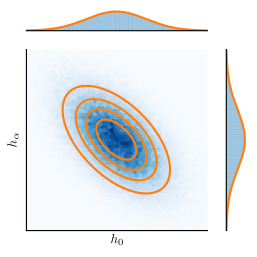
(a)

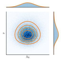
(b)

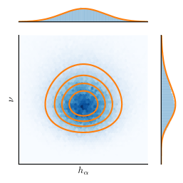
(c)

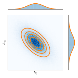
(d)

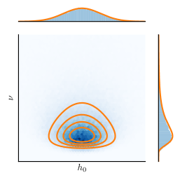
(e)

(f)

Figure 9: The accuracy of our inference algorithm in calculating an approximate surfel model belief (orange), compared against MCMC samples of the exact belief distribution (blue) for a 2-D simulation. We emulate two different sensor modalities: (a-c) a stereo camera by using 100 measurements with high range and low bearing uncertainty, and (d-f) a LiDAR sensor by using 10 measurements with low measurement uncertainty. Shown for these two cases are the three 2-D projections of the 3-D belief distribution over $h_{0}$, $h_{\alpha}$, and $\nu$, and the marginal distributions for each axis. Note that we do not show the axis ticks, as we are only concerned with the relative difference between the exact belief and our approximation.

We have shown that this method of approximation can accurately represent the surfel belief; however, this was only for the case where each surfel is updated in isolation. We will now consider inference on the full model, utilising the approach we have developed here.

5.2 Inference on the Full Model

As opposed to calculating the joint belief distribution over all the surfel parameters in STM map, we instead wish to calculate the marginal belief distributions over each surfel’s parameters. However, as there are shared height parameters between contiguous surfels, we cannot naively use exactly the same approach as we did previously to perform inference on the full model. It should be noted that, although we will consider the joint distribution over all the map parameters, we do not calculate this expressly, as the marginal surfel beliefs are our desired end result.

We can reformulate the inference problem over all the map parameters by utilising our previous approach of performing independent surfel inference. For a given surfel, $s$, we assume that measurements within the associated grid element, $\mathit{Z}_{s}$, and the points on the surface of the environment, $\mathit{M}_{s}$, are independent of all other measurements, $\mathit{Z}\setminus\mathit{Z}_{s}$, and all other surface points, $\mathit{M}\setminus\mathit{M}_{s}$, given the parameters of the surfel, $\bm{\theta}_{s}$. Following this assumption, and using Bayes’ theorem, we can factorise the full joint distribution

$$\begin{split}p(\mathit{\Theta},\mathit{M},\mathit{Z}=\mathtt{Z})&=p(\mathit{\Theta})p(\mathit{M},\mathit{Z}=\mathtt{Z}|\mathit{\Theta})\\ &=p(\mathit{\Theta})\prod_{s\in\mathit{S}}p(\mathit{M}_{s},\mathit{Z}_{s}=\mathtt{Z}_{s}|\bm{\theta}_{s}),\end{split}$$ (57)

where $\mathit{S}$ is the set of all surfels in STM map. Each conditional distribution, $p(\mathit{M}_{s},\mathit{Z}_{s}=\mathtt{Z}_{s}|\bm{\theta}_{s})$, is described by the same model we used previously, namely

$$p(\mathit{M}_{s},\mathit{Z}_{s}=\mathtt{Z}_{s}|\bm{\theta}_{s})=\prod_{i}\phi_{i}(\bm{\theta}_{s},\bm{m}_{i}),$$ (58)

where we again refer to $\phi_{i}(\bm{\theta}_{s},\bm{m}_{i})$ as the likelihood cluster potential—as defined in Equations 13 and 14. We factorise the prior distribution into a product of prior cluster potentials,

$$p(\mathit{\Theta})\propto\prod_{s\in\mathit{S}}\phi_{p}(\bm{\theta}_{s}).$$ (59)

As with our previous approach, each prior cluster potential is distributed according to Equation 28—namely a Gaussian distribution over the vertex heights and an inverse-gamma distribution over the planar deviation. We will examine the effect that this factorisation has on the resulting surfel beliefs, and how the parameter choices (specifically for the height prior distribution) could encode additional structure in the environment (Section 6.1). Combining the prior factorisation with Equation 58, we obtain

$$p(\mathit{\Theta},\mathit{M},\mathit{Z}=\mathtt{Z})=\prod_{s\in\mathit{S}}\phi_{s}(\bm{\theta}_{s},\mathit{M}_{s}),$$ (60)

where the surfel cluster potential, $\phi_{s}(\bm{\theta}_{s},\mathit{M}_{s},\mathit{Z}_{s})$, is calculated according to

$$\begin{split}\phi_{s}(\bm{\theta}_{s},\mathit{M}_{s})&=\phi_{p}(\bm{\theta}_{s})p(\mathit{M}_{s},\mathit{Z}_{s}=\mathtt{Z}_{s}|\bm{\theta}_{s})\\ &=\phi_{p}(\bm{\theta}_{s})\prod_{i}\phi_{i}(\bm{\theta}_{s},\bm{m}_{i}).\end{split}$$ (61)

To calculate a surfel belief for some given measurements, $\mathit{Z}=\mathtt{Z}$, we must marginalise out $\setminus\bm{\theta}_{s}$—all variables except for $\bm{\theta}_{s}$—from the full joint distribution,

$$\begin{split}{\mathcal{B}}(\bm{\theta}_{s})&\propto\int\displaylimits_{\setminus\bm{\theta}_{s}}p(\mathit{\Theta},\mathit{M},\mathit{Z}=\mathtt{Z})\,\text{d}\setminus\bm{\theta}_{s}\\ &=\int\displaylimits_{\setminus\bm{\theta}_{s}}\prod_{s\in\mathit{S}}\phi_{s}(\bm{\theta}_{s},\mathit{M}_{s})\,\text{d}\setminus\bm{\theta}_{s}.\end{split}$$ (62)

The surfel belief can be separated into two terms: one containing the surfel cluster potential of a surfel, $s\in\mathit{S}$, and the other containing the surfel cluster potentials of the rest of surfels, $\mathit{R}=\mathit{S}\setminus s$, namely

$$\begin{split}&{\mathcal{B}}(\mathit{\theta}_{s})\propto\underbrace{\int\displaylimits_{\vphantom{\setminus}\mathit{M}_{s}}\phi_{s}(\bm{\theta}_{s},\mathit{M}_{s})\,\text{d}\mathit{M}_{s}}_{{\phi_{p}(\bm{\theta}_{s})\prod\limits_{i}\delta{{}_{i\shortrightarrow p}}(\bm{\theta}_{s})}}\underbrace{\int\displaylimits_{\setminus\bm{\theta}_{s}}\prod_{r\in\mathit{R}}\phi_{r}(\bm{\theta}_{r},\mathit{M}_{r})\,\text{d}\setminus\bm{\theta}_{s}}_{{\delta{{}_{s\shortleftarrow\mathit{R}}}(\bm{h}_{s})\vphantom{\prod\limits_{i}}}}.\end{split}$$ (63)

The first factor is identical to what was calculated previously when considering each surfel in isolation, with the messages from each likelihood cluster calculated according to Equation 16. We therefore assume that we can calculate this term. The second term is the message from the rest of the surfels in the map, which is due to the shared heights between surfels. This message essentially captures what the rest of the surfels in the map surmise about the heights of the current surfel. Because of the highly coupled nature of the problem, the marginalisation to calculate $\delta{{}_{s\shortleftarrow\mathit{R}}}(\bm{h}_{s})$ is expensive to compute. To keep things tractable, we approximate this message using a technique known as LBP [60]—a message-passing technique that is particularly well suited to calculating approximate marginal distributions without expressly calculating the full joint distribution. LBP is an iterative application of the integral-product algorithm applied to cyclic graphs.

In order to use LBP, we must first construct a cluster graph for the full inference problem. We previously performed inference by only considering each surfel cluster potential when calculating each surfel belief in isolation. We therefore can construct the cluster graph of the full joint distribution, $p(\mathit{\Theta},\mathit{M},\mathit{Z}=\mathtt{Z})$, by repeating the previous cluster graph (Figure 8c) for each surfel in the map, but also creating connections between surfels that share an edge. The resulting cluster graph is illustrated in Figure 10. The scope of the sepset between surfels is generally over the two heights from the shared edge between the surfels—for example $\mathcal{S}_{s,a}=\bm{h}_{s}\cap\bm{h}_{a}$. Although it is not shown explicitly, to ensure a valid cluster graph of the joint distribution it is also necessary to reduce the scope of some sepsets so that the graph obeys the running intersection property, which states that there can only be a single path between the same variable in different parts of the graph. To ensure this property is obeyed, we use the LTRIP algorithm of Streicher and du Preez [61] to construct a cluster graph for the fully-connected model.

(a)

(b)

Figure 10: (a) The cluster graph for the full inference problem shown for a zoomed-in section of STM map. We indicate the sepsets between clusters with $\boxempty$, and each surfel cluster potential with $\bigcirc$. The grey lines indicate the grid elements of the map. (b) We zoom in to the cluster graph, focusing on a specific surfel, $s$, which is contiguous with surfels $a$, $b$ and $c$. The resulting graph is similar to the cluster graph in Figure 8c, but there are now connections between contiguous surfels. The expanded surfel cluster potential $\phi_{s}(\bm{\theta}_{s},\mathit{M}_{s})$ is shown using the dotted outline. The sepset between the surfels is denoted $\mathcal{S}$ (see text for more details on the scope of the sepsets).

From this cluster graph, we can instead calculate an approximation of the message from the rest of the surfels in the map, $\tilde{\delta}{{}_{s\shortleftarrow\mathit{R}}}(\bm{h}_{s})$, by only considering the messages from the subset of surfels that are contiguous to the current surfel, $\mathit{C}\subseteq\mathit{R}$. This results in a much simpler and tractable calculation,

$$\tilde{\delta}{{}_{s\shortleftarrow\mathit{R}}}(\bm{h}_{s})\propto\prod_{c\in\mathit{C}}\delta{{}_{s\shortleftarrow c}}(\mathcal{S}_{s,c}),$$ (64)

where $\mathcal{S}$ denotes the sepset between surfels. It should be noted that the scope of the resulting message might not always contain all the heights in the surfel (as would be the case for surfels on the border of the submap, or if the sepset scope has been reduced to satisfy the running intersection property). Using the integral-product algorithm, LBP defines the iterative update of a message from one surfel, $s$, to another surfel, $a$, according to

$$\begin{split}&\delta{{}_{a\shortleftarrow s}}(\mathcal{S}_{a,s})\propto\int\displaylimits_{\setminus\mathcal{S}_{a,s}}\phi_{p}(\bm{\theta}_{s})\prod\limits_{i}\delta{{}_{i\shortrightarrow p}}(\bm{\theta}_{s})\prod_{c\in\mathit{C}\setminus a}\delta{{}_{s\shortleftarrow c}}(\mathcal{S}_{s,c})\,\text{d}\setminus\mathcal{S}_{a,s}.\end{split}$$ (65)

Using Equation 63, this can be simplified to

$$\begin{split}&\delta{{}_{a\shortleftarrow s}}(\mathcal{S}_{a,s})\propto\int\displaylimits_{\setminus\mathcal{S}_{a,s}}\frac{{\mathcal{B}}(\bm{\theta}_{s})}{\delta{{}_{s\shortleftarrow a}}(\mathcal{S}_{a,s})}\,\text{d}\setminus\mathcal{S}_{a,s}.\end{split}$$ (66)

By iteratively passing these messages between surfels, LBP approximately calculates the marginal belief of each surfel. In order to perform this marginalisation and calculate each surfel belief, the likelihood cluster potentials in each surfel potential need to have a closed-form solution, but this is not the case due to the nonlinearities between the variables in the likelihood cluster potentials. In order to find a closed-form solution to each surfel belief (and consequently the map belief), we again turn to VMP to approximate each likelihood cluster potential; that is, using the local information projection according to Equation 22, repeated here for clarity:

$$\tilde{\phi}_{i}^{*}(\bm{\theta}_{s},\bm{m}_{i})=\operatorname*{arg\,min}_{\tilde{\phi}_{i}\in\mathcal{F}}D_{\text{KL}}\left(\tilde{\phi}_{i}\tilde{\delta}{{}_{i\shortleftarrow p}}\,\middle\|\,\phi_{i}\tilde{\delta}{{}_{i\shortleftarrow p}}\right).$$

However, the approximate incoming message, $\tilde{\delta}{{}_{i\shortleftarrow p}}(\bm{\theta}_{s})$, is now calculated according to

$$\tilde{\delta}{{}_{i\shortleftarrow p}}(\bm{\theta}_{s})=\phi_{p}(\bm{\theta}_{s})\tilde{\delta}{{}_{s\shortleftarrow\mathit{R}}}(\bm{h}_{s})\prod_{j\neq i}\tilde{\delta}{{}_{j\shortrightarrow p}}(\bm{\theta}_{s}).$$ (67)

Similarly to previously—Equation 17—this message is calculated by combining the prior cluster potential, $\phi_{p}(\bm{\theta}_{s})$, with the messages from all other likelihood clusters, $\prod_{j\neq i}\tilde{\delta}{{}_{j\shortrightarrow p}}(\bm{\theta}_{s})$, but now it additionally combines the message from neighbouring surfels, $\tilde{\delta}{{}_{s\shortleftarrow\mathit{R}}}(\bm{h}_{s})$. Using Equation 63, the approximate incoming message can be rewritten in terms of the surfel belief,

$$\tilde{\delta}{{}_{i\shortleftarrow p}}(\bm{\theta}_{s})\propto\frac{\tilde{\mathcal{B}}(\bm{\theta}_{s})}{\tilde{\delta}{{}_{i\shortrightarrow p}}(\bm{\theta}_{s})},$$ (68)

which, in comparison to Equation 67, is cheaper to calculate when iterating over all the measurements. If we combine the prior potential, $\phi_{p}(\bm{\theta}_{s})$, with the incoming message, $\tilde{\delta}{{}_{s\shortleftarrow\mathit{R}}}(\bm{h}_{s})$, into a pseudo-prior, the same approach to what we described previously can be used to perform the local information projection. This specifically includes using the Gaussian family of distributions to model the height distributions, which results in LBP performing approximate inference on only Gaussian distributions—a variant of LBP known as Gaussian LBP. Gaussian LBP is a standard problem formulation for which implementations are available, and we therefore use EMDW—an in-house PGM library. LBP is a tractable approximate inference technique; however, due to its iterative nature, its convergence has not yet been proven. In Gaussian LBP, however, it is known that, if convergence is reached, the posterior means are correct [62, 63]. Although the surfel belief distributions in our problem are not guaranteed to be exactly Gaussian this is a fair assumption as the number of measurements becomes large enough. Additionally, Weiss and Freeman [63] showed that convergence is guaranteed when performing Gaussian LBP on problems with diagonally dominant information matrices. In our problem we expect local regions of the environment to be correlated. Under this assumption, the underlying model should be diagonally dominant. To support this, in our implementation we have not empirically experienced any issues with convergence.

The approach presented here performs inference on STM map using a hybrid message-passing technique using LBP and VMP. Next we provide an overview of the proposed inference algorithm, and discuss some aspects of its implementation.

5.3 Algorithm Overview and Implementation

In Algorithm 1 we describe the process of performing inference given a single batch of measurements. Note that, this could be a batch of measurements accumulated over time, or from a single time step. Notably, 9, 11, 12, 24, 25 and 26 correspond to the LBP update steps, and 14, 15, 17, 19, 21 and 22 to the VMP update steps. We also adjust the method of updating each surfel belief to be more efficient: if only the incoming message from neighbouring surfels has changed during the iterative update process, then it is unnecessary to calculate the updated surfel belief using Equation 63. We instead (equivalently) simplify the update to

$$\tilde{\mathcal{B}}(\bm{\theta}_{s})\triangleq\tilde{\mathcal{B}}(\bm{\theta}_{s})\frac{\tilde{\delta}{{}_{*\shortleftarrow s}}{\mathit{R}}(\bm{h}_{s})}{\tilde{\delta}{{}_{s\shortleftarrow\mathit{R}}}(\bm{h}_{s})},$$ (69)

where we denote the updated and previous incoming messages $\tilde{\delta}{{}_{*\shortleftarrow s}}{\mathit{R}}$ and $\tilde{\delta}{{}_{s\shortleftarrow\mathit{R}}}$ respectively. We next discuss some of the aspects of the algorithm.

Algorithm 1 STM Map Inference

Inputs:
        Prior cluster potentials for each surfel: $\phi_{p}(\bm{\theta}_{s})$ $\forall\,\,s\in\mathit{S}$
        Measurements in each surfel: $\mathtt{Z}_{s}$ $\forall\,\,s\in\mathit{S}$
     Output:
        Surfel beliefs: $\tilde{\mathcal{B}}(\bm{\theta}_{s})$ $\forall\,s\in\mathit{S}$

1:Initialise all messages

2:  $\triangleright$ Initialise all surfel beliefsEquation 63

3:for all $s\in\mathit{S}$ do

4:     $\tilde{\mathcal{B}}(\bm{\theta}_{s})\leftarrow\phi_{p}(\bm{\theta}_{s})\tilde{\delta}{{}_{s\shortleftarrow\mathit{R}}}(\bm{h}_{s})\prod\limits_{i}\tilde{\delta}{{}_{i\shortrightarrow p}}(\bm{\theta}_{s})$

5:end for

6: 

7:repeat$\triangleright$ Cycle through all the surfels in the map

8:     for all $s\in\mathit{S}$ do    $\triangleright$ Calculate the updated incoming message from neighbouring surfelsEquation 64

9:         $\tilde{\delta}{{}_{*\shortleftarrow s}}{R}(\bm{h}_{s})\leftarrow\prod\limits_{c\in\mathit{C}}\delta{{}_{s\shortleftarrow c}}(\mathcal{S}_{s,c})$

10:     $\triangleright$ Update the surfel beliefEquation 69

11:         $\tilde{\mathcal{B}}(\bm{\theta}_{s})\leftarrow\tilde{\mathcal{B}}(\bm{\theta}_{s})\frac{\tilde{\delta}{{}_{*\shortleftarrow s}}{\mathit{R}}(\bm{h}_{s})}{\tilde{\delta}{{}_{s\shortleftarrow\mathit{R}}}(\bm{h}_{s})}$

12:         $\tilde{\delta}{{}_{s\shortleftarrow R}}(\bm{h}_{s})\leftarrow\tilde{\delta}{{}_{*\shortleftarrow s}}{\mathit{R}}(\bm{h}_{s})$

13:     $\triangleright$ Update the likelihood cluster potential for each measurement

14:         for all $\mathtt{z}_{i}\in\mathtt{Z}_{s}$ do         $\triangleright$ Calculate incoming message to the likelihood clusterEquation 68

15:              $\tilde{\delta}{{}_{i\shortleftarrow p}}(\bm{\theta}_{s})\leftarrow\frac{\tilde{\mathcal{B}}(\bm{\theta}_{s})}{\tilde{\delta}{{}_{i\shortrightarrow p}}(\bm{\theta}_{s})}$

16:          $\triangleright$ Update the likelihood cluster potentialSections 5.1.1 and 5.1.2

17:              $\tilde{\phi}_{i}(\bm{h},\bm{m}_{i})\tilde{\phi}_{i}(\nu)\leftarrow\operatorname*{arg\,min}_{\tilde{\phi}_{i}}D_{\text{KL}}\left(\tilde{\phi}_{i}\tilde{\delta}{{}_{i\shortleftarrow p}}\,\middle\|\,\phi_{i}\tilde{\delta}{{}_{i\shortleftarrow p}}\right)$

18:          $\triangleright$ Calculate the outgoing message from the likelihood clusterEquation 16

19:              $\tilde{\delta}{{}_{i\shortrightarrow p}}(\bm{\theta}_{s})\leftarrow\tilde{\phi}_{i}(\nu)\int\tilde{\phi}_{i}(\bm{h},\bm{m}_{i})\,\text{d}\bm{m}_{i}$

20:          $\triangleright$ Update the surfel beliefEquation 21

21:              $\tilde{\mathcal{B}}(\bm{\theta}_{s})\leftarrow\tilde{\delta}{{}_{i\shortrightarrow p}}(\bm{\theta}_{s})\tilde{\delta}{{}_{i\shortleftarrow p}}(\bm{\theta}_{s})$

22:         end for

23:     $\triangleright$ Calculate the outgoing messages to neighbouring surfelsEquation 66

24:         for all $c\in C$ do

25:              $\delta{{}_{c\shortleftarrow s}}(\mathcal{S}_{c,s})=\int\frac{{\mathcal{B}}(\bm{\theta}_{s})}{\delta{{}_{s\shortleftarrow c}}(\mathcal{S}_{c,s})}\,\text{d}\setminus\mathcal{S}_{c,s}$

26:         end for

27:     end for

28:until all messages converge

Message initialisation

We first need to initialise all of the messages before we can begin message passing. In general, the initialisation for iterative approximate inference algorithms can influence the performance, affecting the local optimum to which the algorithm converges, and the convergence speed. We initialise the messages between surfels to be vacuous. For the outgoing messages from each likelihood cluster, we use a simple empirical method of initialisation. Specifically, we initialise each outgoing message, $\tilde{\delta}{{}_{i\shortrightarrow p}}(\bm{h}_{s})$, to have a mean at the $\gamma$ component of the measurement $\mathtt{z}_{i}$, and a (practically) uninformative covariance. This ensures that $\tilde{\mathcal{B}}(\bm{h})$ is initialised to have a mean at the average $\gamma$ component of the measurements. We initialise each outgoing message, $\tilde{\delta}{{}_{i\shortrightarrow p}}(\nu_{s})$, such that the expected value calculated in Equation 38 is the variance of the $\gamma$ component of the measurements.

Incremental updating

During online operation, measurements are received incrementally, and we wish to calculate the surfel beliefs based on all currently available measurements. Ideally, the surfel beliefs should be recalculated as new measurement batches arrive, while also considering all previous measurements. However, as more measurement batches are received, this approach would quickly become intractable. A viable approximation is to only update the outgoing messages from a window of the $W$ latest measurements [64]. Fixing the messages from clusters containing measurements outside this window ensures that updating the surfel belief is linear in the window size $W$. In practice, we combine these constant messages with the prior, discarding the old measurements so that the storage will not grow unbounded. This new prior now summarises all the previous measurements. Following this approach, we can then use the same procedure outlined in Algorithm 1. It should also be noted that previously calculated messages between surfels should not be discarded, but now used as the initialisation for the next batch update.

Convergence

To monitor the state of convergence, we use the fact that all messages will be constant at convergence—that is, convergence has been reached if all messages do not change between iterations. In practice, a message is deemed to be constant if the difference between the successive iterations of the message is negligible. To evaluate this difference, we use the exclusive KL divergence between a message at the current and previous iterations—$D_{\text{KL}}\left(\text{current iteration}\,\middle\|\,\text{previous iteration}\right)$—and the message has converged if the resulting divergence is below a threshold. If all messages related to a surfel have converged, then it is no longer necessary to iterate over it. It should also be noted that, although convergence is not theoretically guaranteed (due to the use of LBP), we have not empirically experienced any issues with convergence in our implementation.

Computational complexity

We can see that the asymptotic computational complexity of our algorithm is $\mathcal{O}(KN)$, where $K$ is the number of iterations in the outermost loop before convergence, and $N$ is the total number of measurements being incorporated into the map. In practice, $K$ is constant with respect to $N$, and therefore the algorithm can be considered approximately linear in $N$. We support this claim with experimental results (Section 6.2).

We have now described performing inference on STM map. Next we look at a series of experiments evaluating the use STM map to represent environments with both simulated and practical data.

6 Experimental Results

Up to this point we have discussed how STM map models the environment, as well as the process of performing inference in the map. We now investigate how the STM mapping technique performs under different experimental conditions. Note that, although we only test STM mapping using data from ground vehicles, it is applicable to all types of autonomous robots: terrestrial, underwater, and aerial.

For the first set of experiments, we use simulated measurement data (Sections 6.1, 6.2 and 6.3). We investigate how the prior distribution parameter choices affect the resulting map (Section 6.1), analyse the cost of performing inference (Section 6.2), and compare the accuracy of STM mapping to elevation mapping (Section 6.3).

We then consider practical datasets collected using either stereo cameras or a LiDAR sensor (Sections 6.4 and 6.5). We demonstrate the modelling performance of the STM mapping technique in relative and global IRF, and perform a qualitative analysis of the resulting STM maps (Sections 6.4 and 6.5 respectively).

6.1 Parameters of the Prior Distribution

In Section 5.1, Equation 28, we gave the form of the prior distribution over the surfel parameters, but did not specify the parameters of the prior distribution. For surfels in the map that contain many measurements, the choice of prior parameters has a negligible effect on the resulting map belief. However, if there are clusters of neighbouring surfels with no measurements, then these surfels’ beliefs are largely determined by the prior distributions.

We want to capture knowledge of the structure of the environment in the prior distribution. The structure we expect is that neighbouring regions tend to have similar heights, which means that we expect neighbouring heights to be positively correlated. If a completely uninformative height prior distribution is used, then only the heights of shared vertices will be affected when performing inference in unobserved regions. In order to achieve this, we use a height prior distribution with covariance,

$$\bm{\Sigma}_{p}=\sigma^{2}\begin{bmatrix}1&\rho&\rho\\ \rho&1&\rho\\ \rho&\rho&1\\ \end{bmatrix},$$ (70)

where $\rho$ is the Pearson correlation coefficient and $\sigma^{2}$ the variance. Without any other information, we expect the heights in a submap to be distributed around the submap plane. We therefore choose the mean of the height prior distribution to represent this initial belief; that is, we set the mean to the zero vector. We choose $\sigma^{2}$ to be uninformative and focus on $\rho$, which should be chosen in the range $\rho\in[0,1)$ to ensure a positively correlated prior distribution. It should be noted that, as the planar deviations in neighbouring surfels are modelled as being statically independent, we model the prior of the planar deviation in a surfel as an uninformative inverse-gamma distribution.

In Figure 11, we show the result of varying the correlation coefficient on the map belief for a 2-D simulation. From this we can see that, by increasing the correlation coefficient, the mean heights of unobserved surfels are affected at an increasing distance from the observed region, which is consistent with smoothly varying environments. We empirically chose $\rho=0.5$, although this choice may vary depending on the nature of the environment. This parameter could conceivably be learnt from data.

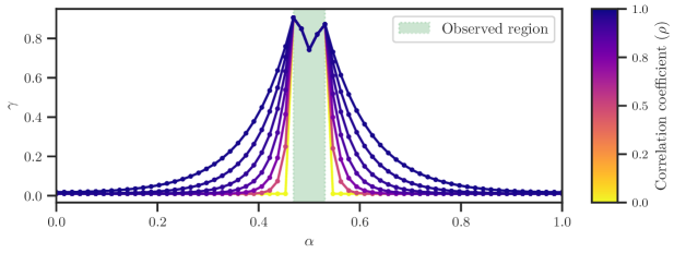
Figure 11: The effect of using a correlated prior distribution when a section of the environment is observed. This is shown for a series of correlation coefficients, spaced using a geometric series: $\{0,2^{-1},2^{-1}+2^{-2},\ldots\}$. Only the mean of the mean mesh belief is shown, and it is coloured according to the correlation coefficient (the darker, the more correlated).

6.2 Cost of Inference

From a tractability perspective, for the STM mapping technique to be viable for online dense mapping, the cost of incorporating one measurement into the map should be constant, irrespective of the size of the map or the number of measurements in the map. This computational requirement is equivalent to the computational complexity of updating the map being linear in the number of measurements, which we previously stated to be true for STM map (Section 5.3). To motivate this statement, we analyse the cost of inference by simulating two scenarios we expect a robot to encounter frequently in practice: incrementally observing new regions of the environment, and re-observing previously observed regions. It should be noted that, to quantify the cost of inference, we count the number of outgoing messages calculated when updating the map (Algorithm 1, 19 and 24). This is an appropriate metric, as it measures the number of iterations for the innermost loops of our inference algorithm.

For both scenarios, we represented the surface of the environment using a 2.5-D surface generated using Perlin noise—a different surface was generated for each scenario. A single submap was used containing $1024$ surfels. Simulated measurements were generated within the relative IRF of the submap by randomly sampling the surface in the observed region (we discuss the sampling strategies further shortly), and then adding zero-mean non-identically distributed Gaussian noise to each sample. The noise covariance was determined by randomly rotating a diagonal covariance matrix. We also ensured that the measurement density in the observed region was approximately uniform and constant across all time steps, at 10 measurements per surfel. Finally, after updating the map at each time step, all the new measurements are windowed.

In the first scenario, we simulated a newly observed region of the environment that shifts incrementally forward–this is typically the case for a robot driving with a 2-D LiDAR sensor mounted in a push-broom configuration. At each time step, simulated measurements are generated from a sampling region (Figure 12a), and the map is updated with the new measurements. The cost of inference for this experiment is shown in Figure 12b. We see that the total number of messages passed at each time step has a linearly decreasing trend, which is expected due to the linearly decreasing sampling region. When we normalise the message counts in each update by the number of new measurements in the update, then this normalised message count is relatively constant. Note that with each incremental update, only local regions of the map were affected significantly (Figure 12c).

(a)

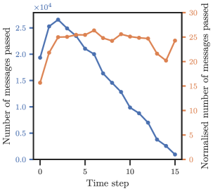
(b)

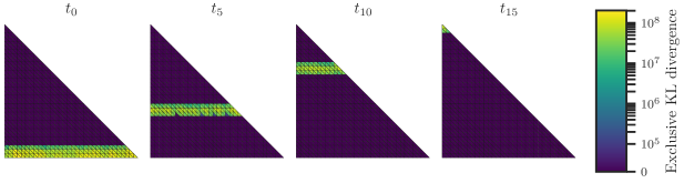
(c)

Figure 12: An experiment showing the cost of inference for the scenario in which new regions of the environment are incrementally observed. (a) The experimental setup showing the sampling regions at selected time steps (green, shaded). Note that the size of the sampling region at each time step decreases linearly. (b) The cost of inference is quantified by the number of messages passed (blue, left axis). This message count is also normalised by the number of new measurements in each update (orange, right axis). (c) To visualise the incremental changes in the surfel beliefs, we calculate the exclusive KL divergence between the surfel beliefs before and after the measurements at a specific time step were incorporated. Note, the colour mapping is scaled using a symmetrical logarithm, which is linear on $[0,10^{5}]$ and logarithmic everywhere else.

In the second scenario, we simulated a region of the environment that is observed repeatedly. This emulates a robot revisiting a previously explored region, or a static robot repeatedly observing the same region. At each time step, simulated measurements are generated by sampling from the entire mapping region. The number of messages passed follows an exponentially decreasing trend (Figure 13); that is, subsequent observations of a previously observed region become computationally cheaper. This is because fewer iterations are required.

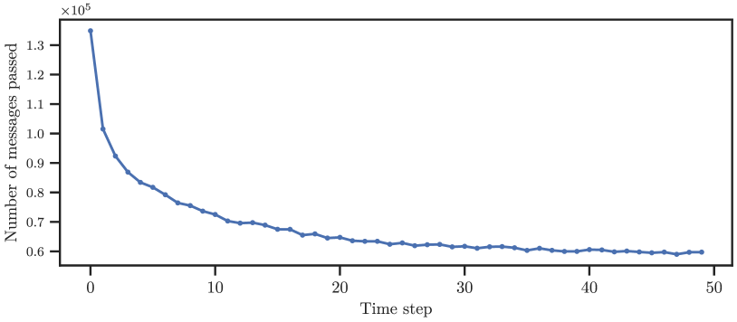
Figure 13: An experiment showing the cost of inference for the scenario in which the same region of the environment is observed repeatedly.

From these two scenarios, we see that updating STM map does indeed have a linear computational cost in the number of measurements, which makes STM mapping a viable online dense mapping technique for the scenarios we expect a robot to encounter in a practical application. We have, however, only analysed the relative computational cost of performing inference on STM map. When considering the absolute computational cost, one of most important aspects is the message and factor dimensionality. In our algorithm, a message passed between neighbouring surfels has at most two dimensions, a message passed within a surfel has three dimensions, and the largest factor has six dimensions. These dimensions are all fixed and relatively low, therefore dimensionality is not a problem for our algorithm. Additionally, although our unoptimised Python implementation takes $\pm 3\text{\,}\mathrm{ms}$ per measurement to update STM map, we expect significantly faster results with an efficient implementation.

6.3 Comparisons of Model Accuracy

STM map is an explicit surface representation that also captures model uncertainty. Therefore, to evaluate the modelling accuracy of STM map, we compare it against a similar class of mapping techniques, namely ones that also use an explicit surface representation and capture model uncertainty. From our summary of the key attributes of the existing mapping techniques (Table 1), the suitable candidate mapping techniques are NDT mapping, GP mapping, and elevation mapping. NDT mapping, however, does not model any measurement uncertainty, and GP mapping is intractable as an online dense mapping technique due to the cubic computational complexity. We therefore only compare STM mapping against standard elevation mapping—that is, each height is updated using a one-dimensional Kalman filter [15, 16].

We perform this comparison using simulated measurement data by quantifying each model’s accuracy against the ground truth using the MSE of each model, and the log-likelihood ratio between both models. Using the same set of measurements, models were built for increasingly finer grid divisions. We first perform this comparison on a 2-D environment, as it is more intuitive to visualise, and we then extend this to a 3-D environment, which is generated using Perlin noise. We also ensured that there were $\pm 10$ measurements per surfel at the finest grid division (for both the 2-D and 3-D experiments).

The results of the 2-D experiment are shown in Figure 13. The MSE of the STM map is better than that of the elevation map for all grid divisions greater than zero. When there is no subdivision (grid division depth = 0), the mean plane of the only surfel in the STM map is almost zero and at the same height as the elevation map (Figure 13c, grid division depth = 0), because the average gradient of the surface of the environment is close to zero. As the grid divisions increase past a certain point, the accuracy of both models begins to degrade (for the MSE, this occurs for grid divisions $>6$ for the STM map and $>7$ for the elevation map). This effect is attributed to the measurement noise (relative to the size of the grid element) becoming too large, and the number of measurements in each grid element decreasing with each grid division. The effect is apparent when looking at the grid division depth of 8 in Figure 13c. From the MSE alone, this result might not appear significant; looking at the log-likelihood ratio shows that, for this environment, the STM map is a more likely model by orders of magnitude. This is as a consequence of the elevation map estimating only the mean height of the surface, whereas the STM map represents the surface as a stochastic process, which is a better representation of the surface of the environment.

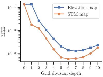
(a)

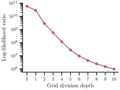
(b)

(c)

Figure 13: An experiment showing a 2-D simulation comparing STM map with the standard elevation map [15, 16]. For increasing grid divisions, we calculate (a) the MSE of each mapping technique compared to the ground-truth surface (lower is better), and (b) the log-likelihood ratio between the STM map and the elevation map is evaluated along the ground-truth surface (lower is better); that is, $\log\text{(\ac{STM} map likelihood})-\log(\text{elevation map likelihood})$. Note that the vertical axis for both comparisons uses a log scale. (c) We also show the ground truth and resulting models for selected grid depths. The shaded regions indicate the one standard deviation confidence intervals in both models (the standard deviations of the elevation map are too small to be seen).

For the 3-D experiment, we ran a batch simulation for 10 synthetically generated environments (Figure 14). Compared to the 2-D experiment, we see a similar trend in the MSE, namely that the STM map is clearly and consistently better than the elevation map for grid division greater than 2. Interestingly, as the grid divisions decrease, there is also a decrease in the batch MSE standard deviation for both models ($>2$ grid divisions). This is because the lower grid divisions are too coarse to effectively represent the environment, and therefore the model accuracy is largely dependent on the particular generated environment. Similarly to the 2-D experiment, the log-likelihood ratio between both models shows that STM map is a significantly better representation than an elevation map.

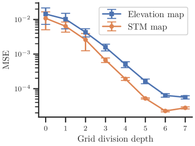
(a)

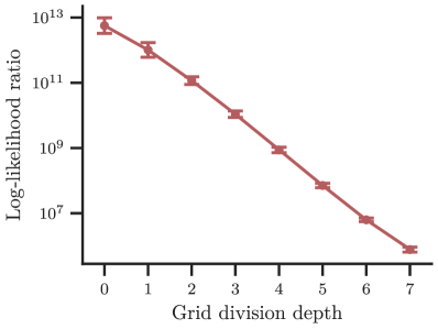
(b)

Figure 14: An experiment showing a 3-D batch simulation ($n=10$) comparing STM map with the standard elevation map [15, 16] for various generated environments. The mean and first standard deviation are shown for (a) the MSE of each mapping technique compared to the ground truth surface, and (b) the log-likelihood ratio between the STM map and the elevation map is evaluated along the ground-truth surface; that is, $\log\text{(\ac{STM} map likelihood})-\log(\text{elevation map likelihood})$.

From these results, we can conclude that, in comparison to a standard elevation map, STM map is a more accurate and better representation of the environment for appropriately chosen grid divisions.

6.4 STM Mapping in a Relative IRF

Although robustly and persistently identifiable landmarks are not currently possible for general environments, there are still viable practical applications using landmark-based relative IRF. In order to demonstrate this, we place artificial landmarks in the environment in the form of ArUco markers [66]—a popular open-source library enabling the creation and detection of binary square fiducial markers. Using these landmarks to define the submapping region, we are able to create STM map using only three pairs of stereo images (Figure 15). The image pairs were synchronously acquired using a stereo setup consisting of two $1.3\text{\,}\mathrm{MP}$ FLIR Flea3 GigE cameras at baseline of $18\text{\,}\mathrm{cm}$. We calculated disparity maps (depth images) from image pairs using the LIBELAS of Geiger et al. [67]. The disparity maps were then transformed to noisy 3-D point measurements using the unscented transform [49]. Following this process, $525\,331$ point measurements were extracted from the three image pairs and incorporated into STM map.

When considering the resulting STM maps, we see that the height maps are visually consistent with the environment. In the rougher regions of the environment (the gravel heap and landmarks in the corners) we see elevated planar deviations, whereas in the smooth regions (the asphalt path) the planar deviations are low. This illustrates the usefulness of the planar deviation in STM map quantifying the surface roughness, which could be used as a measure of terrain drivability. Additionally, despite there being occlusions in the viewpoints (Figures 15c, 15g and 15k), the resulting height maps in these occluded regions are affected by the inference process, and are consistent with a smoothly varying environment. This is due to the correlated prior over the surfel vertex heights (Section 6.1). From this experiment, the resulting map beliefs show that STM map that is visually consistent with the environment can be constructed from only a few viewpoints. This is also performed using stereo camera measurements, which have large range uncertainty.

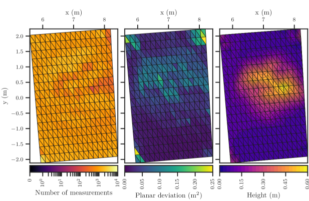
(a)

(b)

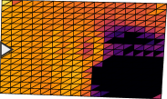
(c)

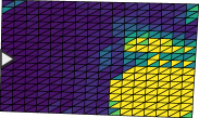
(d)

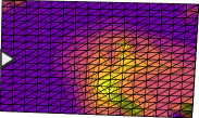
(e)

(f)

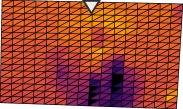
(g)

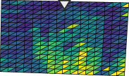
(h)

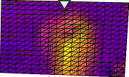
(i)

(j)

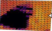
(k)

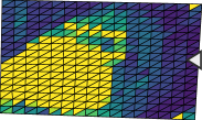
(l)

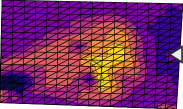
(m)

Figure 15: An experiment showing STM map created using only three pairs of stereo images of an outdoor environment. This was made possible by using relative IRFs to construct two submaps, with artificial ArUco markers [66] as landmarks. Each submap contains 256 surfels. (a) The resulting map is shown for the mean of the mean mesh belief and the planar deviation belief—calculated according to Equation 38. We also show the number of measurements incorporated into each surfel on a symmetrical logarithmic scale, with a linear region on $[0,1]$. (b-m) The STM maps built for each stereo image pair—namely (b-e) a front view, (f-i) a side view, and (j-m) a rear view—are on the same scale as (a). The viewpoints are indicated using arrows. Notably, the occlusions are evident due to a lack of measurements (c, g, k). The orientation of (a) is visually consistent with the front view (b)—that is, a $90\text{\,}\mathrm{\SIUnitSymbolDegree}$ rotation of (c-e).

This test simultaneously demonstrates the success of performing dense mapping in a relative IRF for two practical scenarios: the worst-case SLAM scenario, where there is no information about the robot motion (also commonly known as the kidnapped robot problem [59, chap. 7.1]); as well as the scenario where multiple robots are mapping the same region of the environment. From the perspective of the first scenario, this experiment shows how using a relative IRF fits into the SLAM framework, and how it can perform dense mapping even without any pose information (except that which can be calculated from the landmarks). From the perspective of the second scenario, we illustrate the simplicity of using a relative IRF to perform multi-robot mapping. The maps created from each stereo image pair represent a robot’s perspective (Figures 15b to 15m). As each submap is created relative to the landmarks in the environment, the submaps are already aligned and can be fused together to form a single belief over the environment (Figure 15a).

6.5 STM Mapping in a Global IRF

In order to demonstrate the ability to use STM mapping in a global IRF, we use the Canadian planetary emulation terrain 3-D mapping dataset by Tong et al. [68]. Specifically, we use the box_met dataset taken in the Mars emulation terrain—a $60\text{\times}120\text{\,}\mathrm{m}$ outdoor area. The box_met dataset consists of $19.044\,655\text{\times}{10}^{6}$ LiDAR measurements, taken from 112 poses, and aligned using a DGPS.

In order to construct STM map, a global IRF was created for the rectangular mapping region. The region was subdivided into two submaps, each containing $65\,536$ surfels. From the resulting STM map (Figure 15), we see that the mean mesh belief (Figure 16b) is visually consistent with satellite imagery. From the zoomed-in region (Figure 15d), we see that all the major features visible in the satellite imagery of the environment, even small rocks, are also visible in the map belief. We again see that the planar deviation beliefs (Figure 16c) are visually consistent with the terrain roughness. The steeper regions in the environment, which have a higher planar deviation, also form an outline of the obstacles in the environment. This experiment demonstrates that STM map can be created in a global IRF framework. Although this lacks the benefits of a relative IRF, the added complexity of a relative IRF may not be necessary in situations where the robot localisation is guaranteed to perform accurately; however, this is generally not the case. Additionally, this experiment shows that STM maps can handle datasets with a large number of measurements.

(a)

(b)

(c)

(d)

Figure 15: An experiment showing STM map created in a global IRF using the Canadian planetary emulation terrain 3-D mapping dataset [68]. (a) A satellite view of the mapping region (Google Earth). Note that five zoom regions are demarcated using coloured rectangles and labelled A to E. The resulting map is shown for (b) the mean of the mean mesh belief, and (c) the planar deviation beliefs—calculated according to Equation 38. (d) The map belief for the zoomed regions; they share the same colour maps as in (b, c).

7 Conclusions and Future Work

To address the drawbacks in existing dense mapping techniques, we presented the STM mapping technique, which: represents the structure in the environment using a collection of stochastic processes, forming a continuous representation; is efficient to update, with approximately linear computation time in the number of measurements; is able to handle uncertainty in both measurements and the robot pose; and allows online operation by incrementally updating the map. Although existing techniques have some of these attributes, STM mapping is the only technique that is able to achieve them all. We have shown that STM map is a more accurate and a better representation of the environment in comparison to the standard elevation map [15, 16], when evaluated in terms of MSE and model likelihood. Qualitative results on practical datasets showed that STM maps provide an accurate and descriptive model of the surface of the environment. Additionally, we showed that STM maps are agnostic to the sensor modality, and can handle both accurate (LiDAR) and inaccurate (stereo camera) sensors. Therefore, if a sensor can produce point measurements, it can be used with STM map.

In addition to presenting the STM mapping technique, we have also demonstrated dense mapping using relative IRF in the HYMM submapping framework [2, 3], and extended the framework to 3-D. Using this submapping approach largely decouples the process of localisation from that of dense mapping. This negates some of the issues in performing localisation using SLAM—specifically, it seamlessly allows the incorporation of measurements from multiple robots into a single, consistent representation, mapping between robot poses when the absolute position of the robot is unknown, or mapping when loop closure is performed. The HYMM submapping framework also complements the STM mapping technique, because it uses triangular submapping regions that seamlessly incorporate the triangular surfels in STM map.

7.1 Future Work

The environment often consists of large, homogeneous regions, and naively dividing a dense map into fixed-sized elements is an inefficient use of storage. Therefore, in order for STM maps to better model the environment, future work will look at adaptively subdividing the grid. Surfels with very low planar deviations could be grouped into a coarser resolution and, conversely, surfels with high planar deviations could be subdivided into a finer resolution. This, however, would add complexity to the inference process.

As most environments with practical significance are not static, it would be desirable to relax the static environment assumption. Future work will look at incorporating temporal information into the map to facilitate this.

Although we propose the terrain roughness as a possible metric for drivability analysis, we do not demonstrate this. As a motivation for STM maps to be used in the context of autonomous navigation, future work will look at specialised planning algorithms to exploit the rich environment representation of STM map.

We currently treat each submap independently. However, as each submap lies on a plane defined by the landmarks at its vertices, the partitioning of 3-D space between neighbouring submaps will contain overlapping- or dead-zones. Future work could look at a handling the boundaries between submaps accordingly.

STM map is a 2.5-D representation of the surface of the environment; however, to handle 3-D general environments, future work will look at extending the representation accordingly. As each STM submap is associated to the plane defined by the landmarks vertices, a solution could be to use a more sophisticated strategy of submapping, and then handling the boundaries as mentioned previously. Alternatively, a 3-D triangular meshing strategy could be investigated; however, this will most likely be intractable for online dense mapping if done in a fully probabilistic manner—as with STM mapping.

Our algorithm performs inference on STM map using a combination of both VMP and LBP, and although VMP is guaranteed to converge, LBP on the other hand, does not have any convergence guarantees. We have provided empirical evidence supporting the convergence of our algorithm; however, future work will investigate a principled and in-depth analysis on the convergence of our algorithm.

References

- Guizilini and Ramos [2018] V. Guizilini, F. Ramos, Towards real-time 3D continuous occupancy mapping using Hilbert maps, The International Journal of Robotics Research 37 (2018) 566–584. doi:10.1177/0278364918771476.
- Guivant et al. [2004] J. Guivant, E. Nebot, J. Nieto, F. Masson, Navigation and Mapping in Large Unstructured Environments, The International Journal of Robotics Research 23 (2004) 449–472. doi:10.1177/0278364904042203.
- Nieto et al. [2006] J. Nieto, J. Guivant, E. Nebot, DenseSLAM: Simultaneous Localization and Dense Mapping, The International Journal of Robotics Research 25 (2006) 711–744. doi:10.1177/0278364906067379.
- Thrun et al. [2004] S. Thrun, C. Martin, Y. Liu, D. Hahnel, R. Emery-Montemerlo, D. Chakrabarti, W. Burgard, A Real-Time Expectation-Maximization Algorithm for Acquiring Multiplanar Maps of Indoor Environments With Mobile Robots, IEEE Transactions on Robotics and Automation 20 (2004) 433–442. doi:10.1109/tra.2004.825520.
- Wiemann et al. [2016] T. Wiemann, K. Lingemann, J. Hertzberg, Optimizing Triangle Mesh Reconstructions of Planar Environments, IFAC-PapersOnLine 49 (2016) 218–223. doi:10.1016/j.ifacol.2016.07.735.
- Zienkiewicz et al. [2016] J. Zienkiewicz, A. Tsiotsios, A. Davison, S. Leutenegger, Monocular, Real-Time Surface Reconstruction Using Dynamic Level of Detail, in: 2016 Fourth International Conference on 3D Vision (3DV), IEEE, 2016, pp. 37–46. doi:10.1109/3DV.2016.82.
- Moravec and Elfes [1985] H. Moravec, A. Elfes, High resolution maps from wide angle sonar, in: IEEE International Conference on Robotics and Automation, volume 2, IEEE, 1985, pp. 116–121. doi:10.1109/ROBOT.1985.1087316.
- Hornung et al. [2013] A. Hornung, K. M. Wurm, M. Bennewitz, C. Stachniss, W. Burgard, OctoMap: an efficient probabilistic 3D mapping framework based on octrees, Autonomous Robots 34 (2013) 189–206. doi:10.1007/s10514-012-9321-0.
- Einhorn et al. [2011] E. Einhorn, C. Schroter, H.-M. Gross, Finding the adequate resolution for grid mapping - Cell sizes locally adapting on-the-fly, in: IEEE International Conference on Robotics and Automation, IEEE, 2011, pp. 1843–1848. doi:10.1109/ICRA.2011.5980084.
- Khan et al. [2015] S. Khan, D. Wollherr, M. Buss, Adaptive rectangular cuboids for 3D mapping, in: IEEE International Conference on Robotics and Automation, IEEE, 2015, pp. 2132–2139. doi:10.1109/ICRA.2015.7139480.
- Droeschel et al. [2017] D. Droeschel, M. Schwarz, S. Behnke, Continuous mapping and localization for autonomous navigation in rough terrain using a 3D laser scanner, Robotics and Autonomous Systems 88 (2017) 104–115. doi:10.1016/j.robot.2016.10.017.
- Joubert et al. [2015] D. Joubert, W. Brink, B. Herbst, Pose Uncertainty in Occupancy Grids through Monte Carlo Integration, Journal of Intelligent & Robotic Systems 77 (2015) 5–16. doi:10.1007/s10846-014-0093-y.
- Thrun [2003] S. Thrun, Learning occupancy grid maps with forward sensor models, Autonomous Robots 15 (2003) 111–127. doi:10.1023/A:1025584807625.
- Hebert et al. [1989] M. Hebert, C. Caillas, E. Krotkov, I. Kweon, T. Kanade, Terrain mapping for a roving planetary explorer, IEEE International Conference on Robotics and Automation (1989) 997–1002. doi:10.1109/ROBOT.1989.100111.
- Triebel et al. [2006] R. Triebel, P. Pfaff, W. Burgard, Multi-level surface maps for outdoor terrain mapping and loop closing, in: IEEE International Conference on Intelligent Robots and Systems, IEEE, 2006, pp. 2276–2282. doi:10.1109/IROS.2006.282632.
- Fankhauser et al. [2018] P. Fankhauser, M. Bloesch, M. Hutter, Probabilistic Terrain Mapping for Mobile Robots with Uncertain Localization, IEEE Robotics and Automation Letters 3 (2018) 3019–3026. doi:10.1109/LRA.2018.2849506.
- Marks et al. [2009] T. K. Marks, A. Howard, M. Bajracharya, G. W. Cottrell, L. H. Matthies, Gamma-SLAM: Visual SLAM in unstructured environments using variance grid maps, Journal of Field Robotics 26 (2009) 26–51. doi:10.1002/rob.20273.
- Newcombe et al. [2011] R. A. Newcombe, S. Izadi, O. Hilliges, D. Molyneaux, D. Kim, A. J. Davison, P. Kohli, J. Shotton, S. Hodges, A. Fitzgibbon, KinectFusion: Real-time dense surface mapping and tracking, in: IEEE International Symposium on Mixed and Augmented Reality (ISMAR), 2011, pp. 127–136. doi:10.1109/ISMAR.2011.6092378.
- Whelan et al. [2015] T. Whelan, M. Kaess, H. Johannsson, M. Fallon, J. J. Leonard, J. McDonald, Real-time large-scale dense RGB-D SLAM with volumetric fusion, The International Journal of Robotics Research 34 (2015) 598–626. doi:10.1177/0278364914551008.
- Dai et al. [2017] A. Dai, M. Nießner, M. Zollhöfer, S. Izadi, C. Theobalt, BundleFusion: Real-Time Globally Consistent 3D Reconstruction Using On-the-Fly Surface Reintegration, ACM Transactions on Graphics 36 (2017). doi:10.1145/3054739.
- Dietrich et al. [2016] V. Dietrich, D. Chen, K. M. Wurm, G. v. Wichert, P. Ennen, Probabilistic multi-sensor fusion based on signed distance functions, in: IEEE International Conference on Robotics and Automation, IEEE, 2016. doi:10.1109/icra.2016.7487333.
- Biber and Strasser [2003] P. Biber, W. Strasser, The normal distributions transform: a new approach to laser scan matching, in: IEEE International Conference on Intelligent Robots and Systems, volume 3, IEEE, 2003, pp. 2743–2748. doi:10.1109/IROS.2003.1249285.
- Takeuchi and Tsubouchi [2006] E. Takeuchi, T. Tsubouchi, A 3-D scan matching using improved 3-D normal distributions transform for mobile robotic mapping, in: IEEE International Conference on Intelligent Robots and Systems, IEEE, 2006, pp. 3068–3073. doi:10.1109/IROS.2006.282246.
- Magnusson et al. [2007] M. Magnusson, A. Lilienthal, T. Duckett, Scan Registration for Autonomous Mining Vehicles Using 3D-NDT, Journal of Field Robotics 24 (2007) 803–827. doi:10.1002/rob.
- Stoyanov et al. [2013] T. Stoyanov, M. Magnusson, A. J. Lilienthal, Comparative evaluation of the consistency of three-dimensional spatial representations used in autonomous robot navigation, Journal of Field Robotics 30 (2013) 216–236. doi:10.1002/rob.21446.
- Saarinen et al. [2013] J. P. Saarinen, H. Andreasson, T. Stoyanov, A. J. Lilienthal, 3D normal distributions transform occupancy maps: An efficient representation for mapping in dynamic environments, The International Journal of Robotics Research 32 (2013) 1627–1644. doi:10.1177/0278364913499415.
- Rasmussen and Williams [2006] C. E. Rasmussen, C. K. I. Williams, Gaussian processes for machine learning, MIT Press, 2006.
- Lang et al. [2007] T. Lang, C. Plagemann, W. Burgard, Adaptive Non-Stationary Kernel Regression for Terrain Modeling, in: Robotics: Science and Systems, Robotics: Science and Systems Foundation, 2007. doi:10.15607/rss.2007.iii.011.
- Plagemann et al. [2009] C. Plagemann, S. Mischke, S. Prentice, K. Kersting, N. Roy, W. Burgard, A Bayesian regression approach to terrain mapping and an application to legged robot locomotion, Journal of Field Robotics 26 (2009) 789–811. doi:10.1002/rob.20308.
- Vasudevan [2012] S. Vasudevan, Data fusion with Gaussian processes, Robotics and Autonomous Systems 60 (2012) 1528–1544. doi:10.1016/j.robot.2012.08.006.
- Hadsell et al. [2010] R. Hadsell, J. a. Bagnell, D. Huber, M. Hebert, Space-carving Kernels for Accurate Rough Terrain Estimation, The International Journal of Robotics Research 29 (2010) 981–996. doi:10.1177/0278364910369996.
- O’Callaghan and Ramos [2012] S. T. O’Callaghan, F. T. Ramos, Gaussian process occupancy maps, The International Journal of Robotics Research 31 (2012) 42–62. doi:10.1177/0278364911421039.
- Jadidi et al. [2017] M. G. Jadidi, J. V. Miro, G. Dissanayake, Warped gaussian processes occupancy mapping with uncertain inputs, IEEE Robotics and Automation Letters 2 (2017) 680–687. doi:10.1109/lra.2017.2651154.
- Tresp [2000] V. Tresp, A Bayesian committee machine, Neural Computation 12 (2000) 2719–2741. doi:10.1162/089976600300014908.
- Kim and Kim [2014] S. Kim, J. Kim, Recursive Bayesian updates for occupancy mapping and surface reconstruction, in: Australasian Conference on Robotics and Automation, 2014.
- Wang and Englot [2016] J. Wang, B. Englot, Fast, accurate Gaussian process occupancy maps via test-data octrees and nested Bayesian fusion, in: IEEE International Conference on Robotics and Automation, 2016, pp. 1003–1010. doi:10.1109/ICRA.2016.7487232.
- Ramos and Ott [2016] F. Ramos, L. Ott, Hilbert maps: Scalable continuous occupancy mapping with stochastic gradient descent, The International Journal of Robotics Research 35 (2016) 1717–1730. doi:10.1177/0278364916684382.
- Doherty et al. [2016] K. Doherty, J. Wang, B. Englot, Probabilistic map fusion for fast, incremental occupancy mapping with 3D Hilbert maps, in: IEEE International Conference on Robotics and Automation, 2016, pp. 1011–1018. doi:10.1109/ICRA.2016.7487233.
- Grisetti et al. [2007] G. Grisetti, C. Stachniss, W. Burgard, Improved Techniques for Grid Mapping With Rao-Blackwellized Particle Filters, IEEE Transactions on Robotics 23 (2007) 34–46. doi:10.1109/tro.2006.889486.
- Jones [2006] T. Jones, Tractable Conflict Risk Accumulation in Quadratic Space for Autonomous Vehicles, Journal of Guidance, Control, and Dynamics 29 (2006) 39–48. doi:10.2514/1.10515.
- van Daalen and Jones [2009] C. E. van Daalen, T. Jones, Fast conflict detection using probability flow, Automatica 45 (2009) 1903–1909. doi:10.1016/j.automatica.2009.04.010.
- Engel et al. [2014] J. Engel, T. Schöps, D. Cremers, LSD-SLAM: Large-scale direct monocular SLAM, in: European Conference on Computer Vision, Springer, 2014, pp. 834–849. doi:10.1007/978-3-319-10605-2_54.
- Mur-Artal and Tardós [2017] R. Mur-Artal, J. D. Tardós, ORB-SLAM2: an Open-Source SLAM System for Monocular, Stereo and RGB-D Cameras, IEEE Transactions on Robotics 33 (2017) 1255–1262. doi:10.1109/TRO.2017.2705103.
- Friedman et al. [2007] S. Friedman, H. Pasula, D. Fox, Voronoi Random Fields: Extracting the Topological Structure of Indoor Environments via Place Labeling, in: International Joint Conference on Artifical Intelligence, Morgan Kaufmann Publishers Inc., 2007, pp. 2109–2114.
- Konolige et al. [2011] K. Konolige, E. Marder-Eppstein, B. Marthi, Navigation in hybrid metric-topological maps, in: IEEE International Conference on Robotics and Automation, IEEE, 2011, pp. 3041–3047. doi:10.1109/ICRA.2011.5980074.
- Schmuck et al. [2016] P. Schmuck, S. A. Scherer, A. Zell, Hybrid Metric-Topological 3D Occupancy Grid Maps for Large-scale Mapping, IFAC-PapersOnLine 49 (2016) 230–235. doi:10.1016/j.ifacol.2016.07.738.
- Lowry et al. [2016] S. Lowry, N. Sunderhauf, P. Newman, J. J. Leonard, D. Cox, P. Corke, M. J. Milford, Visual Place Recognition: A Survey, IEEE Transactions on Robotics 32 (2016) 1–19. doi:10.1109/TRO.2015.2496823.
- Julier and Uhlmann [1997] S. J. Julier, J. K. Uhlmann, New extension of the Kalman filter to nonlinear systems, in: Signal Processing, Sensor Fusion, and Target Recognition VI, SPIE, 1997. doi:10.1117/12.280797.
- Julier [2002] S. Julier, The scaled unscented transformation, in: American Control Conference, IEEE, 2002. doi:10.1109/acc.2002.1025369.
- Durrant-Whyte and Bailey [2006] H. Durrant-Whyte, T. Bailey, Simultaneous localization and mapping: part I, IEEE Robotics & Automation Magazine 13 (2006) 99–110. doi:10.1109/MRA.2006.1638022.
- Dissanayake et al. [2001] M. Dissanayake, P. Newman, S. Clark, H. Durrant-Whyte, M. Csorba, A solution to the simultaneous localization and map building (SLAM) problem, IEEE Transactions on Robotics and Automation 17 (2001) 229–241. doi:10.1109/70.938381.
- Koller and Friedman [2009] D. Koller, N. Friedman, Probabilistic graphical models: principles and techniques, MIT Press, 2009.
- Blei et al. [2017] D. M. Blei, A. Kucukelbir, J. D. McAuliffe, Variational Inference: A Review for Statisticians, Journal of the American Statistical Association 112 (2017) 859–877. doi:10.1080/01621459.2017.1285773.
- Minka [2005] T. Minka, Divergence measures and message passing, Technical Report, Technical report, Microsoft Research, 2005.
- Winn and Bishop [2005] J. Winn, C. M. Bishop, Variational Message Passing, Journal of Machine Learning Research 6 (2005) 661–694.
- Minka [2001] T. P. Minka, Expectation propagation for approximate Bayesian inference, in: Uncertainty in Artificial Intelligence, 2001, pp. 362–369.
- Saul and Jordan [1996] L. K. Saul, M. I. Jordan, Exploiting Tractable Substructures in Intractable Networks, in: Advances in Neural Information Processing Systems, MIT Press, 1996, pp. 486–492.
- Bishop [2006] C. M. Bishop, Pattern recognition and machine learning, Springer, 2006.
- Thrun et al. [2005] S. Thrun, W. Burgard, D. Fox, Probabilistic robotics, MIT Press, 2005.
- Frey and MacKay [1998] B. J. Frey, D. J. C. MacKay, A revolution: Belief propagation in graphs with cycles, in: Advances in Neural Information Processing Systems, MIT Press, 1998, pp. 479–485.
- Streicher and du Preez [2017] S. Streicher, J. du Preez, Graph coloring: Comparing cluster graphs to factor graphs, ACM Multimedia 2017 Workshop on South African Academic Participation (2017). doi:10.1145/3132711.3132717.
- Rusmevichientong and Van Roy [2001] P. Rusmevichientong, B. Van Roy, An analysis of belief propagation on the turbo decoding graph with Gaussian densities, IEEE Transactions on Information Theory 47 (2001) 745–765. doi:10.1109/18.910586.
- Weiss and Freeman [2001] Y. Weiss, W. T. Freeman, Correctness of Belief Propagation in Gaussian Graphical Models of Arbitrary Topology, Neural Computation 13 (2001) 2173–2200. doi:10.1162/089976601750541769.
- Qi and Minka [2007] Y. Qi, T. P. Minka, Window-based expectation propagation for adaptive signal detection in flat-fading channels, IEEE Transactions on Wireless Communications 6 (2007) 348–355. doi:10.1109/TWC.2007.05237.
- Perlin [1985] K. Perlin, An image synthesizer, SIGGRAPH Computer Graphics 19 (1985) 287–296. doi:10.1145/325165.325247.
- Garrido-Jurado et al. [2014] S. Garrido-Jurado, R. Muñoz-Salinas, F. J. Madrid-Cuevas, M. J. Marín-Jiménez, Automatic generation and detection of highly reliable fiducial markers under occlusion, Pattern Recognition 47 (2014) 2280–2292. doi:10.1016/j.patcog.2014.01.005.
- Geiger et al. [2011] A. Geiger, M. Roser, R. Urtasun, Efficient large-scale stereo matching, in: Asian Conference on Computer Vision, Springer, 2011, pp. 25–38. doi:10.1007/978-3-642-19315-6_3.
- Tong et al. [2013] C. H. Tong, D. Gingras, K. Larose, T. D. Barfoot, Érick Dupuis, The Canadian planetary emulation terrain 3D mapping dataset, The International Journal of Robotics Research 32 (2013) 389–395. doi:10.1177/0278364913478897.