Span-core Decomposition for Temporal Networks: Algorithms and Applications

Abstract.

When analyzing temporal networks, a fundamental task is the identification of dense structures (i.e., groups of vertices that exhibit a large number of links), together with their temporal span (i.e., the period of time for which the high density holds). In this paper we tackle this task by introducing a notion of temporal core decomposition where each core is associated with two quantities, its coreness, which quantifies how densely it is connected, and its span, which is a temporal interval: we call such cores span-cores.

For a temporal network defined on a discrete temporal domain $T$, the total number of time intervals included in $T$ is quadratic in $|T|$, so that the total number of span-cores is potentially quadratic in $|T|$ as well. Our first main contribution is an algorithm that, by exploiting containment properties among span-cores, computes all the span-cores efficiently. Then, we focus on the problem of finding only the maximal span-cores, i.e., span-cores that are not dominated by any other span-core by both their coreness property and their span. We devise a very efficient algorithm that exploits theoretical findings on the maximality condition to directly extract the maximal ones without computing all span-cores.

Finally, as a third contribution, we introduce the problem of temporal community search, where a set of query vertices is given as input, and the goal is to find a set of densely-connected subgraphs containing the query vertices and covering the whole underlying temporal domain $T$. We derive a connection between this problem and the problem of finding (maximal) span-cores. Based on this connection, we show how temporal community search can be solved in polynomial-time via dynamic programming, and how the maximal span-cores can be profitably exploited to significantly speed-up the basic algorithm.

We provide an extensive experimentation on several real-world temporal networks of widely different origins and characteristics. Our results confirm the efficiency and scalability of the proposed methods. Moreover, we showcase the practical relevance of our techniques in a number of applications on temporal networks, describing face-to-face contacts between individuals in schools. Our experiments highlight the relevance of the notion of (maximal) span-core in analyzing social dynamics, detecting/correcting anomalies in the data, and graph-embedding-based network classification.

1. Introduction

A temporal network is a representation of entities (vertices), their relations (links), and how these relations are established/broken over time. Notice that here we will consider discrete times, i.e., the temporal networks can be represented as a time-ordered series of snapshots (instantaneous graphs). Extracting dense structures (i.e., groups of vertices exhibiting a large number of links with each other), together with their temporal span (i.e., the period of time for which the high density is observed) is a key mining primitive to characterize such temporal networks and extract relevant structures. This type of pattern enables fine-grain analysis of the network dynamics and can be a building block towards more complex tasks and applications, such as finding temporally recurring subgraphs or anomalously dense ones. For instance, they can help in studying contact networks among individuals to quantify the transmission opportunities of respiratory infections in a population and uncover situations where the risk of transmission is higher, with the goal of designing mitigation strategies (Gemmetto et al., 2014). Anomalously dense temporal patterns among entities in a co-occurrence graph (e.g., extracted from the Twitter stream) have also been used to identify events and buzzing stories in real time (Angel et al., 2012; Bonchi et al., 2016, 2019). Another example concerns scientific collaboration and citation networks, where these patterns can help understand the dynamics of collaboration in successful professional teams, study the evolution of scientific topics, and detect emerging technologies (Érdi et al., 2013).

In this paper we adopt as a measure of density of a pattern the minimum degree holding among the vertices in the subgraph during the pattern’s span. The problem of extracting all these patterns is tackled by introducing a notion of temporal core decomposition in which each core is associated with its span, i.e., an interval of contiguous timestamps, for which the coreness property holds. We term such a notion of temporal core span-core.

Moreover, in several application scenarios it is typically required to identify only those dense patterns that contain a given set of query vertices. We therefore introduce the problem of temporal community search, whose goal is to find a set of cohesive temporal subgraphs containing the input query vertices and covering the whole temporal domain.

To the best of our knowledge, the problems of (efficient) span-core computation and temporal community search have never been studied so far.

1.1. Challenges and contributions

As the number of possible time intervals is quadratic in the size of the input temporal domain $T$, the total number of span-cores is, in the worst case, quadratic in $T$ too. The naive method to find all span-cores, which would be to operate a core decomposition for each of these time intervals, would therefore be very time-consuming. This is a major challenge that we tackle by deriving containment properties between span-cores and by exploiting them to devise an algorithm for computing all the span-cores that is significantly more efficient than the naïve exhaustive method.

We then shift our attention to the problem of finding only the maximal span-cores, defined as the span-cores that are not dominated by any other span-core by both the coreness property and the span. A straightforward way of approaching this problem is to filter out non-maximal span-cores during the execution of an algorithm for computing the whole span-core decomposition. However, as the maximal ones are usually much less numerous than the overall span-cores, it would be desirable to have a method that effectively exploits the maximality property and extracts maximal span-cores directly, without computing the complete decomposition. The design of an algorithm of this kind is an interesting challenge, as it contrasts with the intrinsic conceptual properties of core decomposition, based on which a core of order $k$ can be efficiently computed from the core of order $k\!-\!1$, of which it is a subset. For this reason, at first glance, the computation of the core of the highest order would seem as hard as computing the overall core decomposition. Instead, in this work we derive a number of theoretical properties about the relationship among span-cores of different temporal intervals and, based on these findings, we show how such a challenging goal may be achieved.

Finally, we focus on the problem of community search in temporal networks. Community search has been extensively studied in static graphs. It requires to find a subgraph containing a given set of query vertices and maximizing a certain density measure (Fang et al., 2020; Huang et al., 2017). Here, we propose a formulation of the community-search problem in temporal networks as follows: given a set $Q$ of query vertices, and a positive integer $h$, find a segmentation of the underlying temporal domain in $h$ segments $\{\Delta_{i}\}_{i=1}^{h}$ and a subgraph $S_{i}$ for every identified segment $\Delta_{i}$ such that each $S_{i}$ contains the query vertices $Q$ and the total density of the subgraphs is maximized. Following the bulk of the literature in community search on static networks, in our definition of temporal community search we adopt the minimum degree as a density measure.

We show that, with some manipulations, temporal community search can be reformulated as an instance of the popular sequence segmentation problem, which asks for partitioning a sequence of numerical values into $h$ segments so as to minimize the sum of the penalties (according to some penalty function) on the identified segments (Bellman, 1961). Therefore, the classical dynamic-programming algorithm for sequence segmentation by Bellman (Bellman, 1961) can be easily adapted to solve temporal community search in polynomial time.

A criticality of this approach is that a naïve adaptation of the Bellman’s algorithm takes quadratic time in the size of the input temporal domain $T$. As a major contribution in this regard, we prove that the set of maximal span-cores provide a sound and complete basis to still have an optimal solution to temporal community search, while at the same time leading to a significant speed-up with respect to the naïve method. In fact, let $T^{*}\subseteq T$ be the subset of timestamps that are covered by the span of at least one maximal span-core, together with the timestamps that immediately precede or succeed any of such spans. We show that considering $T^{*}$ (instead of $T$) in the (adaptation of the) Bellman’s algorithm is sufficient to optimally solve the underlying temporal-community-search problem instance. As, typically, $|T^{*}|\ll|T|$, this finding guarantees a considerable improvement in efficiency (as confirmed by our experiments).

A further challenge in our temporal-community-search problem is a typical one in community-search formulations based on minimum degree, namely, that the output subgraphs are typically large in size. We tackle this challenge by devising a method to reduce the size of the output subgraphs without affecting optimality. The proposed method is inspired by the one devised by Barbieri et al. (Barbieri et al., 2015) for the problem of minimum community search (in static graphs).

To summarize, the main contributions of this paper are as follows:

• We introduce the notion of span-core decomposition and maximal span-core in temporal networks, characterizing structure and size of the search space and providing important containment properties (Section 3).

• We devise an algorithm for computing all span-cores that exploits the aforementioned containment properties and is orders of magnitude faster than a naïve method based on traditional core decomposition (Section 4).

• We study the problem of finding only the maximal span-cores. We derive several theoretical findings about the relationship between maximal span-cores and exploit these findings to devise an algorithm that is more efficient than computing all span-cores and discarding the non-maximal ones (Section 5).

• We introduce the problem of temporal community search and show how it can be solved in polynomial time via dynamic programming. We prove an important connection between temporal community search and maximal span-cores, which allows us to devise an algorithm that is considerably more efficient than the naïve dynamic-programming one. We also propose a method to achieve the critical challenge of having too large communities as output (Section 6).

• We provide a comprehensive experimentation on several real-world temporal networks, with millions of vertices, tens of millions of edges, and hundreds of timestamps, which attests efficiency and scalability of our methods (Section 7).

• We present applications on face-to-face interaction networks that illustrate the relevance of the notions of (maximal) span-core and temporal community search in real-life analyses and applications (Section 8).

The next section provides an overview of the related literature, while Section 9 discusses future work and concludes the paper.

An abridged version of this work, covering Sections 4 and 5, together with the corresponding experiments (i.e., parts of Sections 7 and 8), was presented in (Galimberti et al., 2018).

Reproducibility. For the sake of reproducibility, all our code and some of the datasets used in this paper are available at github.com/egalimberti/span_cores.

2. Background and related work

2.1. Core decomposition

Given a simple (static) graph $G=(V,E)$, let $d(S,u)$ denote the degree of vertex $u\in V$ in the subgraph induced by vertex set $S\subseteq V$, i.e., $d(S,u)=|\{v\in S\mid(u,v)\in E\}|$. The notions of $k$-core and core decomposition are defined as follows:

Definition 1 ($k$-core and core decomposition (Matula and Beck, 1983)).

The $k$-core (or core of order $k$) of $G$ is a maximal set of vertices $C_{k}\subseteq V$ such that $\forall u\in C_{k}:d(C_{k},u)\geq k$. The set of all $k$-cores $V=C_{0}\supseteq C_{1}\supseteq\cdots\supseteq C_{k^{*}}$ ($k^{*}=\arg\max_{k}C_{k}\neq\emptyset$) is the core decomposition of $G$.

Core decomposition can be computed in linear time by iteratively removing the smallest-degree vertex and setting its core number as equal to its degree at the time of removal (Batagelj and Zaversnik, 2011). Among the many definitions of dense structures, core decomposition is particularly appealing as, among others, it is fast to compute, and can speed-up/approximate dense-subgraph extraction according to various other definitions. For instance, core decomposition allows for finding cliques more efficiently (Eppstein et al., 2010), as a $k$-clique is contained into a $(k\!-\!1)$-core, which can be significantly smaller than the original graph. Moreover, core decomposition is at the basis of approximation algorithms for the densest-(at-least-$k$-)subgraph problem (Kortsarz and Peleg, 1994; Andersen and Chellapilla, 2009), and betweenness centrality (Healy et al., 2006). Core decomposition has also been recognized as an important tool to analyze and visualize complex networks (Batagelj et al., 1999; Alvarez-Hamelin et al., 2006) in several domains, e.g., bioinformatics (Bader and Hogue, 2003; Wuchty and Almaas, 2005), software engineering (Zhang et al., 2010), and social networks (Kitsak et al., 2010; García et al., 2013). It has been studied under various settings, such as distributed (Montresor et al., 2013), streaming/maintenance (Sariyüce et al., 2013; Li et al., 2014), and disk-based (Cheng et al., 2011), and generalized to various types of static graphs, such as uncertain (Bonchi et al., 2014), directed (Giatsidis et al., 2013), weighted (Garas et al., 2012; Eidsaa and Almaas, 2013), bipartite graphs (Liu et al., 2019b), or including attributes on the nodes (Zhang et al., 2017). For a comprehensive survey about theory, algorithms, and applications of core decomposition we refer to (Bonchi et al., 2018; Malliaros et al., 2020).

Two types of extension of core decomposition bear some relation to our work. First, core decomposition in multilayer networks – i.e., networks that are composed of a superposition of networks – has been studied in (Galimberti et al., 2017; Galimberti et al., 2020). In the multilayer setting a core is allowed to extend on any subset of layers, thus implying that the total number of multilayer cores is exponential in the number of layers. Although temporal networks can be viewed as a special case of multilayer networks (where each timestamp is interpreted as a layer), there is a fundamental difference: in a temporal network the “layers” are ordered, and the sequentiality of timestamps represents an important structural constraint. In other words, in the temporal setting we are interested in cores that span a temporal interval, and not simply any subset of (potentially non-contiguous) timestamps. This aspect has two critical consequences. First, the search space and the number of temporal cores are no longer exponential, unlike the multilayer case. Second, to guarantee an effective fulfilment of the constraint on temporal sequentiality, the requirements for the edges that contribute to the formation of a temporal core are stricter than the ones at the basis of the multilayer-core definition. A more detailed technical discussion of the relationship between multilayer core decomposition and the proposed temporal core decomposition is reported in Section 3.3.

The second extension of core decomposition that shares some relation to the one proposed in this work is due to Wu et al., who have proposed in (Wu et al., 2015) an alternative definition of temporal core decomposition. A major difference between Wu et al.’s definition and ours is that the former does not take any kind of temporal constraint into account. Indeed, Wu et al. define the $(k,h)$-core as the largest subgraph in which every vertex has at least $k$ neighbors and there are at least $h$ temporal edges between the vertex and its neighbors, without any restriction on when these $h$ edges occur: the sequentiality of connections is not taken into account and non-contiguous timestamps can support the same core. In fact, the $(k,h)$-core decomposition can be seen as a kind of weighted static core decomposition on the weighted static network resulting from the aggregation of the temporal network. In contrast, our temporal cores have each a clear temporal collocation and continuous spans, so that our definition includes temporality in an explicit way and cannot be reduced to Wu et al.’s one. As we will see in Section 8, associating a temporal collocation to each core is important in applications.

2.2. Patterns in temporal networks

A number of works on extracting dense patterns from a temporal network focus on the well-established notion of densest subgraph, i.e., a subgraph maximizing the average-degree density. Jethava and Beerenwinkel (Jethava and Beerenwinkel, 2015) consider as input a set of graphs sharing the same vertex set, which can thus also be interpreted as a temporal network. On such an input they study the densest common subgraph problem, i.e., the problem of finding a subgraph maximizing the minimum average degree over all graphs (timestamps), and devise a linear-programming formulation and a greedy heuristic algorithm for it. Further (mostly theoretical) advancements to the densest-common-subgraph problem have been provided by Reinthal et al. (Reinthal et al., 2016) and Charikar et al. (Charikar et al., 2018). Semertzidis et al. (Semertzidis et al., 2018) instead introduce two more variants of the problem, where the goal is to maximize the average average degree and the minimum minimum degree, respectively. They show that the average-average variant easily reduces to the traditional densest-subgraph problem, and that the minimum-minimum variant can be exactly solved by a simple adaptation of the classic algorithm for core decomposition.

Complementary works focus on variants of the densest-subgraph-discovery problem. Rozenshtein et al. study the problem of discovering dense temporal subgraphs whose edges occur in short time intervals considering the exact timestamp of the occurrences (Rozenshtein et al., 2017), and the problem of partitioning the timeline of a temporal network into non-overlapping intervals, such that the intervals span subgraphs with maximum total density (Rozenshtein et al., 2018). Epasto et al. (Epasto et al., 2015) deal with the problem of maintaining the densest subgraph in a dynamic setting.

Attention in the literature has also been devoted to densities other than the average degree. The notion of $\Delta$-clique, as a set of vertices in which each pair is in contact at least every $\Delta$ timestamps, has been proposed in (Viard et al., 2016; Himmel et al., 2016). Bentert et al. (Bentert et al., 2018) introduce the $\Delta$-$k$-plex, a relaxation of $\Delta$-clique in which each vertex has an edge to all but at most $k-1$ vertices at least once every $\Delta$ consecutive timestamps. Li et al. (Li et al., 2018) study the problem of finding the maximum ($\theta$,$\Delta$)-persistent $k$-core in a temporal network, i.e., the largest subgraph that is a connected $k$-core in all the subintervals of duration $\theta$ of a given temporal interval $\Delta$.

A different, but still slightly related body of literature focuses on other definitions of temporal patterns, such as frequent evolution patterns in temporal attributed graphs (Berlingerio et al., 2009; Inokuchi and Washio, 2010; Desmier et al., 2012), link-formation rules in temporal networks (Bringmann et al., 2010; Leung et al., 2010), frequency-estimation algorithms for counting temporal motifs (Kovanen et al., 2011; Liu et al., 2019a), finding a small vertex set whose removal eliminates all temporal paths connecting two designated terminal vertices (Zschoche et al., 2020), finding a subgraph that maximizes the sum of edge weights in a network whose topology remains fixed but edge weights evolve over time (Bogdanov et al., 2011; Ma et al., 2017), and the discovery of dynamic relationships and events (Das Sarma et al., 2011), or of correlated activity patterns (Gauvin et al., 2014).

This work differs from all the above ones as our notions of span-core and temporal core decomposition do not correspond (or are straightforwardly reducible) to any of those temporal patterns.

2.3. Community search

Given a static graph and a set of query vertices, the community search problem aims at finding a cohesive subgraph containing the query vertices. Community search has attracted a great deal of attention in the last years (Fang et al., 2020; Huang et al., 2017). Sozio and Gionis (Sozio and Gionis, 2010) are the first to introduce this problem by employing the minimum degree as a cohesiveness measure. Their formulation can be solved by a simple (linear-time) greedy algorithm, which resembles the traditional $2$-approximation algorithm for densest subgraph proposed in (Charikar, 2000). More recently, Cui et al. (Cui et al., 2014) devise a local-search approach to improve the efficiency of the method defined in (Sozio and Gionis, 2010), but only for the special case of a single query vertex. The case of multiple query vertices has instead been addressed by Barbieri et al. (Barbieri et al., 2015), who exploit core decomposition as a preprocessing step to improve efficiency. They also tackle the problem of minimum community search, i.e., a variant of community search where the size of the output subgraph has to be minimized.

Community search has also been studied under different names and/or settings. Huang et al. (Huang et al., 2014) introduce a community-search model based on the $k$-truss notion. Andersen and Lang (Andersen and Lang, 2006) and Kloumann and Kleinberg (Kloumann and Kleinberg, 2014) study seed set expansion in social graphs, in order to find communities with small conductance or that are well-resemblant of the characteristics of the query vertices, respectively. Other works define connectivity subgraphs based on electricity analogues (Faloutsos et al., 2004), random walks (Tong and Faloutsos, 2006), the minimum-description-length principle (Akoglu et al., 2013), the Wiener index (Ruchansky et al., 2015) and network efficiency (Ruchansky et al., 2017). Recent approaches also introduce the flexibility of having query vertices belonging to different communities (Bian et al., 2018; Yan et al., 2019). Finally, community search has been formalized for attributed graphs (Huang and Lakshmanan, 2017; Fang et al., 2017a) and spatial graphs (Fang et al., 2017b) as well.

In this work we study for the first time community search in temporal graphs. Specifically, we provide a novel definition of the problem by asking for a set of subgraphs containing the given query vertices, along with their corresponding temporal intervals, such that the total minimum-degree density of the identified subgraphs is maximized and the union of the temporal intervals spanned by those subgraphs covers the whole underlying temporal domain. None of the above works deal with such a definition of temporal community search, not even the works by Rozenshtein et al. (Rozenshtein et al., 2018) and Li et al. (Li et al., 2018) discussed in the previous subsection. In fact, although Rozenshtein et al. (Rozenshtein et al., 2018) and Li et al. (Li et al., 2018) search for cohesive temporal subgraphs, they do not accept any query vertices in input. This is a fundamental feature, which makes those works actually solve a problem other than community search. Another key difference is that they focus on different notions of density.

3. Temporal core decomposition: problem statement

In this section we provide preliminary definitions and the needed notations, introduce the problem of finding all span-cores and only the maximal ones, and prove containment properties among span-cores that are at the basis of our efficient algorithms.

3.1. Span-cores

We are given a temporal graph $G=(V,T,\tau)$, where $V$ is a set of vertices, $T=[0,1,\ldots,t_{max}]\subseteq\mathbb{N}$ is a discrete time domain, and $\tau:V\times V\times T\rightarrow\{0,1\}$ is a function defining for each pair of vertices $u,v\in V$ and each timestamp $t\in T$ whether edge $(u,v)$ exists in $t$. We denote $E=\{(u,v,t)\mid\tau(u,v,t)=1\}$ the set of all temporal edges. Given a timestamp $t\in T$, $E_{t}=\{(u,v)\mid\tau(u,v,t)=1\}$ is the set of edges existing at time $t$. A temporal interval $\Delta=[t_{s},t_{e}]$ is contained into another temporal interval $\Delta^{\prime}=[t^{\prime}_{s},t^{\prime}_{e}]$, denoted $\Delta\sqsubseteq\Delta^{\prime}$, if $t^{\prime}_{s}\leq t_{s}$ and $t^{\prime}_{e}\geq t_{e}$. Given an interval $\Delta\sqsubseteq T$, we denote $E_{\Delta}=\bigcap_{t\in\Delta}E_{t}$ the edges existing in all timestamps of $\Delta$. Given a subset $S\subseteq V$ of vertices, let $E_{\Delta}[S]=\{(u,v)\in E_{\Delta}\mid u\in S,v\in S\}$ and $G_{\Delta}[S]=(S,E_{\Delta}[S])$. Finally, the temporal degree of a vertex $u$ within $G_{\Delta}[S]$ is denoted $\mbox{$d$}_{\Delta}(S,u)=|\{v\in S\mid(u,v)\in E_{\Delta}[S]\}|$.

Definition 2 ($(k,\Delta)$-core).

The $(k,\Delta)$-core of a temporal graph $G=(V,T,\tau)$ is (when it exists) a maximal and non-empty set of vertices $\emptyset\neq C_{k,\Delta}\subseteq V$, such that $\forall u\in C_{k,\Delta}:\mbox{$d$}_{\Delta}(C_{k,\Delta},u)\geq k$, where $\Delta\sqsubseteq T$ is a temporal interval and $k\in\mathbb{N}^{+}$.

A $(k,\Delta)$-core is thus a set of vertices implicitly defining a cohesive subgraph (where $k$ represents the cohesiveness constraint), together with its temporal span, i.e., the interval $\Delta$ for which the subgraph satisfies the cohesiveness constraint. In the remainder of the paper we refer to this type of temporal pattern as span-core.

The first problem we tackle in this work is to compute the span-core decomposition of a temporal graph $G$, i.e., all span-cores of $G$.

Problem 1 (Span-core decomposition).

Given a temporal graph $G$, find the set of all $(k,\Delta)$-cores of $G$.

Unlike standard cores of simple graphs, span-cores are not all nested into each other, due to their spans. However, they still exhibit containment properties. Indeed, it can be observed that a $(k,\Delta)$-core is contained into any other $(k^{\prime},\Delta^{\prime})$-core with less restrictive degree and span conditions, i.e., $k^{\prime}\leq k$, and $\Delta^{\prime}\sqsubseteq\Delta$. This property is depicted in Figure 1, and formally stated in the next proposition.

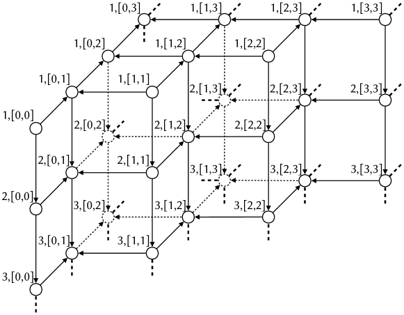
Figure 1. Search space: for a temporal span $\Delta=[t_{s},t_{e}]$, the $(k,\Delta)$-core is depicted as a node labeled “$k,[t_{s},t_{e}]$”. An arrow $C_{1}\rightarrow C_{2}$ denotes $C_{1}\supseteq C_{2}$ (the distinction between solid and dotted arrows is for visualization sake only).

Proposition 1 (Span-core containment).

For any two span-cores $C_{k,\Delta}$, $C_{k^{\prime},\Delta^{\prime}}$ of a temporal graph $G$ it holds that

$$k^{\prime}\leq k\wedge\Delta^{\prime}\sqsubseteq\Delta\ \Rightarrow\ C_{k,\Delta}\subseteq C_{k^{\prime},\Delta^{\prime}}.$$

Proof.

The result can be proved by separating the two conditions in the hypothesis, i.e., by separately showing that ($i$) $k^{\prime}\leq k\Rightarrow C_{k,\Delta}\subseteq C_{k^{\prime},\Delta}$, and ($ii$) $\Delta^{\prime}\sqsubseteq\Delta\Rightarrow C_{k,\Delta}\subseteq C_{k,\Delta^{\prime}}$. The first point holds as, keeping the span $\Delta$ fixed, the maximal set of vertices $C$ for which $\mbox{$d$}_{\Delta}(C,u)\geq k$ is clearly contained in the maximal set of vertices $C^{\prime}$ for which $\mbox{$d$}_{\Delta}(C^{\prime},u)\geq k^{\prime}$, if $k^{\prime}\leq k$. To prove (ii), it can be noted that $\Delta^{\prime}\sqsubseteq\Delta\Rightarrow E_{\Delta}\subseteq E_{\Delta^{\prime}}$, which implies that $\forall u\in C_{k,\Delta}:\mbox{$d$}_{\Delta}(C_{k,\Delta},u)\leq\mbox{$d$}_{\Delta^{\prime}}(C_{k,\Delta},u)$. Therefore, all vertices within $C_{k,\Delta}$ satisfy the condition to be part of $C_{k,\Delta^{\prime}}$ too. ∎

The following observation directly derives from Proposition 1 and states that finding all the span-cores having a fixed span $\Delta$ corresponds to computing the core decomposition of a simple graph.

Observation 1.

For a fixed temporal interval $\Delta\sqsubseteq T$, finding all span-cores that have $\Delta$ as their span is equivalent to computing the classic core decomposition (Batagelj and Zaversnik, 2011) of the simple graph $G_{\Delta}=(V,E_{\Delta})$.

3.2. Maximal span-cores

As the total number of temporal intervals that are contained into the whole time domain $T$ is $|T|(|T|\!+\!1)/2$, the total number of span-cores is potentially $\mathcal{O}(|T|^{2}\times k_{max})$, where $k_{max}$ is the largest value of $k$ for which a $(k,\Delta)$-core exists. It is thus quadratic in $|T|$, which may be too large an output for human direct inspection. In this regard, it may be useful to focus only on the most relevant cores, i.e., the maximal ones, as defined next.

Definition 3 (Maximal span-core).

A span-core $C_{k,\Delta}$ of a temporal graph $G$ is said maximal if there does not exist any other span-core $C_{k^{\prime},\Delta^{\prime}}$ of $G$ such that $k\leq k^{\prime}$ and $\Delta\sqsubseteq\Delta^{\prime}$.

Hence, a span-core is recognized as maximal if it is not dominated by another span-core both on the order $k$ and the span $\Delta$. Differently from the innermost core (i.e., the core of the highest order) in the classic core decomposition, which is unique, in our temporal setting the number of maximal span-cores is $\mathcal{O}(|T|^{2})$, as, in the worst case, there may be one maximal span-core for every temporal interval. However, as observed in empirical temporal-network data, maximal span-cores are always much less than the overall span-cores: the difference is usually one order of magnitude or more. The second problem we tackle in this work is to compute the maximal span-cores of a temporal graph.

Problem 2 (Maximal Span-core Mining).

Given a temporal graph $G$, find the set of all maximal $(k,\Delta)$-cores of $G$.

Clearly, one could solve Problem 2 by solving Problem 1 and filtering out all the non-maximal span-cores. However, an interesting yet challenging question is whether one can exploit the maximality condition to develop faster algorithms that can directly extract the maximal ones, without computing all the span-cores. We provide a positive answer to this question in Section 5.

3.3. Relation to multilayer core decomposition (Galimberti et al., 2017; Galimberti et al., 2020)

Multilayer graphs are a representation paradigm of complex systems, where multiple relations of different types occur between the same pair of entities (Bonchi et al., 2015; Dickison et al., 2016; Tagarelli et al., 2017). A multilayer graph is formally defined as a triple $G=(V,E,L)$, where $V$ is a set of vertices, $L$ is a set of layers, and $E\subseteq V\times V\times L$ is a set of edges. Given a multilayer graph $G=(V,E,L)$ and an $|L|$-dimensional integer vector $\vec{k}=[k_{\ell}]_{\ell\in L}$, Galimberti et al. (Galimberti et al., 2017; Galimberti et al., 2020) define the notion of multilayer $\vec{k}$-core of $G$ as a maximal set $C\subseteq V$ of vertices such that, for all $\ell\in L$, the minimum degree of a vertex in $C$ in layer $\ell$ is larger than or equal to $k_{\ell}$. In other words, a $\vec{k}$-multilayer-core corresponds to a subgraph that satisfies the $k_{\ell}$-core definition in layer $\ell$, for all $\ell\in L$. For instance, for $|L|=2$, a multilayer $(k_{1},k_{2})$-core is a subgraph that is simultaneously a $k_{1}$-core in the first layer and a $k_{2}$-core in the second layer.

Temporal graphs can be viewed as a special case of multilayer graphs where timestamps correspond to layers. Therefore, a natural question while introducing a notion of temporal core is how it relates to the definition of a core in the multilayer setting. A fundamental difference is that, unlike the multilayer context, in a temporal graph the “layers” are ordered, and the consecutio of timestamps should be taken into account. As a result, the two definitions are not comparable and have different conceptual and computational properties in the general case. A major remark in this regard is that the multilayer cores, as defined in (Galimberti et al., 2017; Galimberti et al., 2020), are exponential in the number $|L|$ of layers $|L|$, thus the multilayer core decomposition takes (worst-case) exponential time, while temporal core decomposition is computable in polynomial time.

Once having ascertained such a key difference, another meaningful investigation would be understanding whether the notion of multilayer core may still be exploited to define/compute span-cores, even if only in limited circumstances. In this regard, as formally shown in the next proposition and illustrated in the example in Figure 2, there exists a containment relationship between span-cores and multilayer cores.

Proposition 2.

Let $C$ be the $(k,\Delta)$-span-core of a temporal graph $G=(V,T,\tau)$. Let also $\vec{k}=[k_{t}]_{t\in T}$ be a $|T|$-dimensional integer vector such that $\forall t\in\Delta:k_{t}=k$, $\forall t\notin\Delta:k_{t}=0$, and let $C^{\prime}$ be the $\vec{k}$-multilayer-core extracted from $G$ by interpreting it as a multilayer graph where layers correspond to timestamps. It holds that $C\subseteq C^{\prime}$.

Proof.

According to Definition 2, every vertex $v\in C$, has a at least $k$ neighbors within $C\setminus\{v\}$, for every timestamp $t\in\Delta$. This complies with the definition of $\vec{k}$-multilayer-core, $\vec{k}=[k_{t}]_{t\in T}$, $\forall t\in\Delta:k_{t}=k$, $\forall t\notin\Delta:k_{t}=0$, meaning that all vertices in $C$ are necessarily part of the $\vec{k}$-multilayer-core as well. ∎

Figure 2. Relationship between multilayer cores defined in (Galimberti et al., 2017; Galimberti et al., 2020) and span-cores introduced in this work (Proposition 2). The figure depicts a toy temporal graph $G$, with time domain $T=\{0,1,2\}$. Solid, dashed, and dotted edges refer to timestamp $0$, $1$, and $2$, respectively. The $(2,[0,1])$-span-core of $G$ corresponds to $C=\{\mbox{{A,D,E}}\}$. At the same time, $C^{\prime}=\{\mbox{{A,B,D,E}}\}$ corresponds to the $(2,2,0)$-multilayer-core of $G$, when $G$ is interpreted as a (3-layer) multilayer graph with the first, second, and third layer corresponding to timestamps $0$, $1$, and $2$, respectively. While there is no exact correspondence, it can be observed that span-core $C$ is contained into multilayer core $C^{\prime}$.

Proposition 2 suggests that, in principle, to compute span-cores, one may: ($i$) compute all multilayer cores, ($ii$) among all multilayer cores, retrieve the ones complying with Proposition 2, and ($iii$) post-process those multilayer cores in order to extract the actual span-cores. However, this strategy is not feasible, as, due to the aforementioned exponential-time computation, extracting multilayer cores from a temporal graph would be affordable only for very small values of $|T|$. In fact, Galimberti et al. (Galimberti et al., 2017; Galimberti et al., 2020) show experiments on graphs with at most 10 layers, and in the 10-layer graphs computing the multilayer core decomposition takes more than 28 hours. In the temporal setting we are interested in analyzing long-term, sometimes high-frequency, interactions, thus temporal graphs have typically much more than 10 timestamps. Indeed, all the datasets used in this paper have many more timestamps, and the algorithms from (Galimberti et al., 2017; Galimberti et al., 2020) cannot run in a reasonable amount of time. Moreover, even assuming to be able to compute multilayer cores on temporal networks, those cores have still to be filtered and post-processed, which makes this strategy meaningless with respect to methods that compute span-cores directly, as the ones introduced in the next section.

4. Algorithms: computing all span-cores

In this section we devise algorithms for computing a complete span-core decomposition of a temporal graph (Problem 1).

A naïve approach. As stated in Observation 1, for a fixed temporal interval $\Delta\sqsubseteq T$, mining all span-cores $C_{k,\Delta}$ is equivalent to computing the classic core decomposition of the graph $G_{\Delta}=(V,E_{\Delta})$. A naïve strategy is thus to run a core-decomposition subroutine (Batagelj and Zaversnik, 2011) on graph $G_{\Delta}$ for each temporal interval $\Delta\sqsubseteq T$. Such a method has time complexity $\mathcal{O}(\sum_{\Delta\sqsubseteq T}(|\Delta|\times|E|))$, i.e., $\mathcal{O}(|T|^{2}\times|E|)$.

A more efficient algorithm. Looking at Figure 1 one can observe that the naïve algorithm only exploits one dimension of the containment property: it starts from each point on the top level, i.e., from cores of order $1$, and goes down vertically with the classic core decomposition. Based on Proposition 1, it is possible to design a more efficient algorithm that exploits also the “horizontal containment” relationships.

Example 1.

Consider core $C_{1,[0,2]}$ in Figure 1: by Proposition 1 it holds that it is a subset of both $C_{1,[0,1]}$ and $C_{1,[1,2]}$. Therefore, to compute $C_{1,[0,2]}$, instead of starting from the whole $V$, one can start from $C_{1,[0,1]}\cap C_{1,[1,2]}$. Starting from a much smaller set of vertices can provide a substantial speed-up to the whole computation.

This observation, although simple, produces a speed-up of orders of magnitude as we will empirically show in Section 7. The next straightforward corollary of Proposition 1 states that, not only $C_{1,[0,2]}\subseteq C_{1,[0,1]}\cap C_{1,[1,2]}$, but this is the best one can get, meaning that intersecting these two span-cores is equivalent to intersecting all span-cores structurally containing $C_{1,[0,2]}$.

Corollary 1.

Given a temporal graph $G=(V,T,\tau)$, and a temporal interval $\Delta=[t_{s},t_{e}]\sqsubseteq T$, let $\Delta_{+}=[\min\{t_{s}+1,t_{e}\},t_{e}]$ and $\Delta_{-}=[t_{s},\max\{t_{e}-1,t_{s}\}]$. It holds that

$$C_{1,\Delta}\ \subseteq\ (C_{1,\Delta_{+}}\cap C_{1,\Delta_{-}})\ =\ \bigcap_{\Delta^{\prime}\sqsubseteq\Delta}C_{1,\Delta^{\prime}}.$$

Example 2.

Consider again $C_{1,[0,2]}$ in Figure 1: Proposition 1 states that it is a subset of $C_{1,[0,0]},C_{1,[0,1]},C_{1,[1,1]},C_{1,[1,2]},C_{1,[2,2]}$. Corollary 1 suggests that there is no need to intersect them all, but only $C_{1,[0,1]}$ and $C_{1,[1,2]}$: in fact, $C_{1,[0,1]}\subseteq C_{1,[0,0]}\cap C_{1,[1,1]}$ and $C_{1,[1,2]}\subseteq C_{1,[1,1]}\cap C_{1,[2,2]}$.

Input: A temporal graph $G=(V,T,\tau)$.

Output: The set $\mathbf{C}$ of all span-cores of $G$.

1 $\mathbf{C}\leftarrow\emptyset$;   $Q\leftarrow\emptyset$;   $\mathcal{A}\leftarrow\emptyset$

2 forall $t\in T$ do

3       enqueue $[t,t]$ to $Q$;   $\mathcal{A}[t,t]\leftarrow V$

4      

5while $Q\neq\emptyset$ do

6       dequeue $\Delta=[t_{s},t_{e}]$ from $Q$

7       $E_{\Delta}[\mathcal{A}[\Delta]]\leftarrow\{(u,v)\in E_{\Delta}\mid u\in\mathcal{A}[\Delta],v\in\mathcal{A}[\Delta]\}$

8      

9      if $|E_{\Delta}[\mathcal{A}[\Delta]]|>0$ then

10             $\mathbf{C}_{\Delta}\leftarrow$ core-decomposition$(\mathcal{A}[\Delta],E_{\Delta}[\mathcal{A}[\Delta]])$

11             $\mathbf{C}\leftarrow\mathbf{C}\cup\mathbf{C}_{\Delta}$

12             $\Delta_{1}=[\max\{t_{s}-1,0\},t_{e}]$;    $\Delta_{2}=[t_{s},\min\{t_{e}+1,t_{max}\}]$

13             forall $\Delta^{\prime}\in\{\Delta_{1},\Delta_{2}\}\mid\Delta^{\prime}\neq\Delta$ do

14                   if $\mathcal{A}[\Delta^{\prime}]\neq\textsc{null}$ then

15                         $\mathcal{A}[\Delta^{\prime}]\leftarrow\mathcal{A}[\Delta^{\prime}]\cap C_{1,\Delta}$

16                         enqueue $\Delta^{\prime}$ to $Q$

17                        

18                   else

19                         $\mathcal{A}[\Delta^{\prime}]\leftarrow C_{1,\Delta}$

20                        

21                  

22            

23      

Algorithm 1 Span-cores

The main idea behind our efficient Span-cores algorithm (whose pseudocode is given as Algorithm 1) is to generate temporal intervals of increasing size (starting from size one) and, for each $\Delta$ of width larger than one, to initiate the core decomposition from $(C_{1,\Delta_{+}}\cap C_{1,\Delta_{-}})$, i.e., the smallest intersection of cores containing $C_{1,\Delta}$ (Corollary 1). The intervals to be processed are added to queue $Q$, which is initialized with the intervals of size one (Lines 1–1): these are the only intervals for which no other interval can be used to reduce the set of vertices from which the core decomposition is started, thus they have to be initialized with the whole vertex set $V$. The algorithm utilizes a map $\mathcal{A}$ that, given an interval $\Delta$, returns the set of vertices to be used as a starting set of the core decomposition on $\Delta$. The algorithm processes all intervals stored in $Q$, until $Q$ has become empty (Lines 1–1). For every temporal interval $\Delta$ extracted from $Q$, the starting set of vertices is retrieved from $\mathcal{A}[\Delta]$ and the corresponding set of edges is identified (Line 1). Unless this is empty, the classic core-decomposition algorithm (Batagelj and Zaversnik, 2011) is invoked over $(\mathcal{A}[\Delta],E_{\Delta}[\mathcal{A}[\Delta]])$ (Line 1) and its output (a set of span-cores of span $\Delta$) is added to the ultimate output set $\mathbf{C}$ (Line 1).

Afterwards, the two intervals, denoted $\Delta_{1}$ and $\Delta_{2}$, for which $C_{1,\Delta}$ can be used to obtain the smallest intersections of cores containing them (Corollary 1) are computed at Line 1. For $\Delta_{1}$ (and analogously $\Delta_{2}$), we check whether $\mathcal{A}[\Delta_{1}]$ has already been initialized (Line 1): this would mean that previously the other “father” (i.e., smallest containing core) of $C_{1,\Delta_{1}}$ has been computed, thus we can intersect $C_{1,\Delta}$ with $\mathcal{A}[\Delta_{1}]$ and enqueue $\Delta_{1}$ to be processed (Lines 1–1). Instead, if $\mathcal{A}[\Delta_{1}]$ was not yet initialized, we initialize it with $C_{1,\Delta}$ (Line 1): in this case $\Delta_{1}$ is not enqueued because it still lacks one father to be intersected before being ready for core decomposition. This procedural update of $Q$ ensures that both fathers of every interval in $Q$ exist and have been previously computed, thus no a-posteriori verification is needed.

Example 3.

Consider again the search space in Figure 1. Algorithm 1 first processes the intervals $[0,0],[1,1],[2,2],$ and $[3,3]$. Then, it intersects $C_{1,[0,0]}$ and $C_{1,[1,1]}$ to initialize $C_{1,[0,1]}$, intersects $C_{1,[1,1]}$ and $C_{1,[2,2]}$ to initialize $C_{1,[1,2]}$, and intersects $C_{1,[2,2]}$ and $C_{1,[3,3]}$ to initialize $C_{1,[2,3]}$. Then, it continues with the intervals of size 3: it intersects $C_{1,[0,1]}$ and $C_{1,[1,2]}$ to initialize $C_{1,[0,2]}$ and so on.

The next theorem formally shows soundness and completeness of our Span-cores algorithm.

Theorem 1.

Algorithm 1 is sound and complete for Problem 1.

Proof.

The algorithm generates and processes a subset of temporal intervals $\mathcal{X}\subseteq\{\Delta\mid\Delta\sqsubseteq T\}$. For every interval $\Delta\subseteq\mathcal{X}$, it computes all span-cores $\mathbf{C}_{\Delta}=\{C_{1,\Delta},C_{2,\Delta},\ldots,C_{k_{\Delta},\Delta}\}$ defined on $\Delta$ by means of the core-decomposition subroutine on the graph $(\mathcal{A}[\Delta],E_{\Delta}[\mathcal{A}[\Delta]])$. The set of vertices $\mathcal{A}[\Delta]$ is equivalent to $(C_{1,\Delta_{+}}\cap C_{1,\Delta_{-}})$ because of Line 1 (Corollary 1) and the fact that $\Delta$ is enqueued (Line 1) only when both fathers have been processed and the intersection done. The correctness of doing the classic core decomposition is guaranteed by Observation  1.

As for completeness, it suffices to show that the intervals $\Delta\notin\mathcal{X}$ that have not been processed by the algorithm do not yield any span-core. The algorithm generates all temporal intervals size by size, starting from those of size one and then going to larger sizes. This is done by maintaining the queue $Q$. As said above, an interval $\Delta$ is enqueued as soon as both $C_{1,\Delta_{+}}$ and $C_{1,\Delta_{-}}$ have been processed. Thus, an interval $\Delta$ is not in $\mathcal{X}$ only if either $C_{1,\Delta_{+}}$ or $C_{1,\Delta_{-}}$ does not exist. In this case $C_{1,\Delta}$ and all other $C_{k,\Delta}$ do not exist as well. ∎

Discussion. Algorithm 1 exploits the “horizontal containment” relationships only at the first level of the search space. For a given $\Delta$, once the restricted starting set of vertices has been defined for $k=1$, the traditional core decomposition is started to produce all the span-cores of span $\Delta$. In other words, for $k>1$ only the “vertical containment” is exploited. Consider the span-core $C_{3,[1,2]}$ in Figure 1: we know that it is a subset of $C_{2,[1,2]}$ (“vertical” ) and of $C_{3,[1,1]}$ and $C_{3,[2,2]}$ (“horizontal” ). One could consider intersecting all these three span-cores before computing $C_{3,[1,2]}$. We tested this alternative approach, but concluded that the overhead of computing intersections and data-structure maintenance was outweighing the benefit of starting from a smaller vertex set.

The worst-case time complexity of Algorithm 1 is equal to the naïve approach, however, in practice, it is orders of magnitude faster, as shown in Section 7.

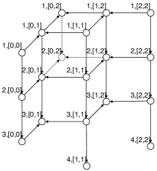
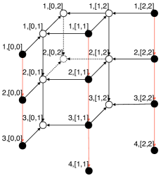
(a)	(b)	(c)
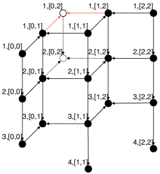
(d)	(e)	(f)

Figure 3. Run-through example of the execution of Span-cores (Algorithm 1) over the search space of a temporal graph having $T=[0,2]$. Full nodes represent computed span-cores, while empty nodes are span-cores that will be visited in the next steps of the algorithm. Red arrows highlight the containment relationships exploited during the current step.

Example 4.

Figure 3 reports a run-through example, illustrating the execution of Span-cores (Algorithm 1) over the search space of a toy temporal graph having $T=[0,2]$ (shown in Figure 3(a)). The algorithm starts by computing all the span-cores having span of size 1 (Figure 3(b)); in this case, only the “vertical containment” is exploited by the core-decomposition subroutine. Then, Span-cores  proceeds with the computation of the span-cores having span of size 2. At first, the algorithm exploits the “horizontal containment” relationships at the first level of the search space to restrict the starting set of vertices for computing the span-cores of $k=1$ (Figure 3(c)). Afterwards, the core-decomposition subroutine computes all the span-cores with span of size 2, by following the “vertical containment” (Figure 3(d)). Finally, the same method is applied for visiting the span-cores with span of size 3 (Figure 3(e)-(f)).

5. Algorithms: computing maximal span-cores

In this section we focus on Problem 2: computing the maximal span-cores of a temporal graph.

A filtering approach. As anticipated above, a straightforward way of solving this problem consists in filtering the span-cores computed during the execution of Algorithm 1, so as to ultimately output only the maximal ones. This can easily be accomplished by equipping Algorithm 1 with a data structure $\mathcal{M}$ that stores the span-core of the highest order for every temporal interval $\Delta\sqsubseteq T$ that has been processed by the algorithm. Moreover, at the storage of a span-core $C_{k,\Delta}$ in $\mathcal{M}$, the span-cores previously stored in $\mathcal{M}$ for subintervals of the temporal interval $\Delta$ and with the same order $k$ are removed from $\mathcal{M}$. This removal operation, together with the order in which span-cores are processed, ensures that $\mathcal{M}$ eventually contains only the maximal span-cores.

Efficient maximal-span-core finding. Our next goal is to design a more efficient algorithm that extracts maximal span-cores directly, without computing complete core decompositions, passing over more peripheral ones, and without generating all temporal cores. This is a quite challenging design principle, as it contrasts the intrinsic structural properties of core decomposition, based on which a core of order $k$ is usually computed from the core of order $k\!-\!1$, thus making the computation of the core of the highest order as hard as computing the overall decomposition. Nevertheless, thanks to theoretical properties that relate the maximal span-cores to each other, in the temporal context such a challenge can be achieved. In the following we discuss such properties in detail, by starting from a result that has already been discussed above, but only informally.

Consider the classic core decomposition in a standard (non-temporal) graph $G$ (Definition 1) and let $C_{k^{*}}[G]$ denote the innermost core of $G$, i.e., the non-empty $k$-core of $G$ with the largest $k$.

Lemma 1.

Given a temporal graph $G=(V,T,\tau)$, let $\mathbf{C}_{M}$ be the set of all maximal span-cores of $G$, and $\mathbf{C_{inner}}=\{C_{k^{*}}[G_{\Delta}]\mid\Delta\sqsubseteq T\}$ be the set of innermost cores of all graphs $G_{\Delta}$. It holds that $\mathbf{C}_{M}\subseteq\mathbf{C_{inner}}$.

Proof.

Every $C_{k,\Delta}\in\mathbf{C}_{M}$ is the innermost core of the non-temporal graph $G_{\Delta}$: else, there would exist another core $C_{k^{\prime},\Delta}\neq\emptyset$ with $k^{\prime}>k$, implying that $C_{k,\Delta}\notin\mathbf{C}_{M}$. ∎

Lemma 1 states that each maximal span-core is an innermost core of a $G_{\Delta}$, for some temporal interval $\Delta\sqsubseteq T$. Hence, there can exist at most one maximal span-core for every $\Delta\sqsubseteq T$ (while an interval $\Delta$ may not yield any maximal span-core). The key question to design an efficient maximal-span-core-mining algorithm thus becomes how to extract innermost cores of the graphs $G_{\Delta}$ more efficiently than by computing the full core decompositions of all $G_{\Delta}$. The answer to this question comes from the result stated in the next two lemmas (with Lemma 2 being auxiliary to Lemma 3).

Lemma 2.

Given a temporal graph $G=(V,T,\tau)$, and three temporal intervals $\Delta=[t_{s},t_{e}]\sqsubseteq T$, $\Delta^{\prime}=[t_{s}\!-\!1,t_{e}]\sqsubseteq T$, and $\Delta^{\prime\prime}=[t_{s},t_{e}\!+\!1]\sqsubseteq T$. The innermost core $C_{k^{*}}[G_{\Delta}]$ is a maximal span-core of $G$ if and only if $k^{*}>\max\{k^{\prime},k^{\prime\prime}\}$ where $k^{\prime}$ and $k^{\prime\prime}$ are the orders of the innermost cores of $G_{\Delta^{\prime}}$ and $G_{\Delta^{\prime\prime}}$, respectively.

Proof.

The “$\Rightarrow$” part comes directly from the definition of maximal span-core (Definition 3): if $k^{*}$ were not larger than $\max\{k^{\prime},k^{\prime\prime}\}$, then $C_{k^{*}}[G_{\Delta}]$ would be dominated by another span-core both on the order and on the span (as both $\Delta^{\prime}$ and $\Delta^{\prime\prime}$ are superintervals of $\Delta$). For the “$\Leftarrow$” part, from Lemma 1 and Proposition 1 it follows that $\max\{k^{\prime},k^{\prime\prime}\}$ is an upper bound on the maximum order of a span-core of a superinterval of $\Delta$. Therefore, $k^{*}>\max\{k^{\prime},k^{\prime\prime}\}$ implies that there cannot exist any other span-core that dominates $C_{k^{*}}[G_{\Delta}]$ both on the order and on the span. ∎

Lemma 3.

Given $G$, $\Delta$, $\Delta^{\prime}$, $\Delta^{\prime\prime}$, $k^{\prime}$, and $k^{\prime\prime}$ defined as in Lemma 2, let $\widetilde{V}=\{u\in V\mid\mbox{$d$}_{\Delta}(V,u)>\max\{k^{\prime},k^{\prime\prime}\}\}$, and let $C_{k^{*}}[G_{\Delta}[\widetilde{V}]]$ be the innermost core of $G_{\Delta}[\widetilde{V}]$. If $k^{*}>\max\{k^{\prime},k^{\prime\prime}\}$, then $C_{k^{*}}[G_{\Delta}[\widetilde{V}]]$ is a maximal span-core; otherwise, no maximal span-core exists for $\Delta$.

Proof.

Lemma 2 states that, to be recognized as a maximal span-core, the innermost core of $G_{\Delta}$ should have order larger than $\max\{k^{\prime},k^{\prime\prime}\}$. This means that, if the innermost core of $G_{\Delta}$ is a maximal span-core, all vertices $u\notin\widetilde{V}$ cannot be part of it. Therefore, $G_{\Delta}$ yields a maximal span-core only if the innermost core of subgraph $G_{\Delta}[\widetilde{V}]$ has order $k^{*}>\max\{k^{\prime},k^{\prime\prime}\}$. ∎

Lemma 3 provides the basis of our efficient method for extracting maximal span-cores. Basically, it states that, to verify whether a certain temporal interval $\Delta=[t_{s},t_{e}]$ yields a maximal span-core (and, if so, compute it), there is no need to consider the whole graph $G_{\Delta}$, rather it suffices to start from a smaller subgraph, which is given by all vertices whose temporal degree is larger than the maximum between the orders of the innermost cores of intervals $\Delta^{\prime}=[t_{s}\!-\!1,t_{e}]$ and $\Delta^{\prime\prime}=[t_{s},t_{e}\!+\!1]$. This finding suggests a strategy that is opposite to the one used for computing the overall span-core decomposition: a top-down strategy that processes temporal intervals starting from the larger ones. Indeed, in addition to exploiting the result in Lemma 3, this way of exploring the temporal-interval space allows us to skip the computation of complete core decompositions of the whole “singleton-interval” graphs $\{G_{{}_{[t,t]}}\}_{t\in T}$, which may easily become a critical bottleneck, as they are the largest ones among the graphs induced by temporal intervals.

Input: A temporal graph $G=(V,T,\tau)$.

Output: The set $\mathbf{C}_{M}$ of all maximal span-cores of $G$.

1

2$\mathbf{C}_{M}\leftarrow\emptyset$

3 $\mathcal{K}^{\prime}[t]\leftarrow 0$, $\forall t\in T$

4

5forall $t_{s}\in[0,1,\ldots,t_{max}]$ do

6       $t^{*}\leftarrow\max\{t_{e}\in[t_{s},t_{max}]\mid E_{{}_{[t_{s},t_{e}]}}\neq\emptyset\}$

7       $k^{\prime\prime}\leftarrow 0$

8       forall $t_{e}\in[t^{*},t^{*}\!-\!1,\ldots,t_{s}]$ do

9             $\Delta\leftarrow[t_{s},t_{e}]$

10             $lb\leftarrow\max\{\mathcal{K}^{\prime}[t_{e}],k^{\prime\prime}\}$

11             $V_{lb}\leftarrow\{u\in V\mid\mbox{$d$}_{\Delta}(V,u)>lb\}$

12             $E_{\Delta}[V_{lb}]\leftarrow\{(u,v)\in E_{\Delta}\mid u\in V_{lb},v\in V_{lb}\}$

13             $C\leftarrow$ innermost-core$(V_{lb},E_{\Delta}[V_{lb}])$

14             $k^{*}\leftarrow$ order of $C$

15             if $k^{*}>lb$ then

16                   $\mathbf{C}_{M}\leftarrow\mathbf{C}_{M}\cup\{C\}$

17                  

18            $k^{\prime\prime}\leftarrow\max\{k^{\prime\prime},k^{*}\}$;  $\mathcal{K}^{\prime}[t_{e}]\leftarrow\max\{\mathcal{K}^{\prime}[t_{e}],k^{\prime\prime}\}$

19            

20      

Algorithm 2 Maximal-span-cores

The Maximal-span-cores algorithm. Algorithm 2 iterates over all timestamps $t_{s}\in T$ in increasing order (Line 2), and for each $t_{s}$ it first finds all the maximal span-cores that have span starting in $t_{s}$. This way of proceeding ensures that a span-core that is recognized as maximal will not be later dominated by another span-core. Indeed, an interval $[t_{s},t_{e}]$ can never be contained in another interval $[t_{s}^{\prime},t_{e}^{\prime}]$ with $t_{s}<t_{s}^{\prime}$. For a given $t_{s}$, all maximal span-cores are computed as follows. First, the maximum timestamp $\geq t_{s}$ such that the corresponding edge set $E_{{}_{[t_{s},t_{e}]}}$ is not empty is identified as $t^{*}$ (Line 2). Then, all intervals $\Delta=[t_{s},t_{e}]$ are considered one by one in decreasing order of $t_{e}$ (Lines 2–2): this again guarantees that a span-core that is recognized as maximal will not be later dominated by another span-core, as the intervals are processed from the largest to the smallest. At each iteration of the internal cycle, the algorithm resorts to Lemma 3 and computes the lower bound $lb$ on the order of the innermost core of $G_{\Delta}$ to be recognized as maximal, by taking the maximum between $\mathcal{K}^{\prime}[t_{e}]$ and $k^{\prime\prime}$ (Line 2). $\mathcal{K}^{\prime}$ is a map that maintains, for every timestamp $t\in[t_{s},t^{*}]$, the order of the innermost core of graph $G_{\Delta^{\prime}}$, where $\Delta^{\prime}=[t_{s}\!-\!1,t]$ (i.e., $\mathcal{K}^{\prime}[t]$ stores what in Lemmas 2–3 is denoted as $k^{\prime}$). Whereas $k^{\prime\prime}$ stores the order of the innermost core of $G_{\Delta^{\prime\prime}}$, where $\Delta^{\prime\prime}=[t_{s},t_{e}+1]$. Afterwards, the sets of vertices $V_{lb}$ and of edges $E_{\Delta}[V_{lb}]$ that comply with this lower-bound constraint are built (Lines 2–2), and the innermost core of the subgraph $(V_{lb},E_{\Delta}[V_{lb}])$ is extracted (Lines 2–2). Ultimately, based again on Lemma 3, such a core is added to the output set of maximal span-cores only if its order is actually larger than $lb$ (Lines 2–2), and the values of $k^{\prime\prime}$ and $\mathcal{K}^{\prime}[t_{e}]$ are updated (Line 2). Specifically, note that the order $k^{*}$ of core $C$ may in principle be less than $k^{\prime\prime}$, as $C$ is extracted from a subgraph of $G_{\Delta}$. If this happens, it means that the actual order of the innermost core of $G_{\Delta}$ is equal to $k^{\prime\prime}$. This motivates the update rules (and their order) reported in Line 2.

Theorem 2.

Algorithm 2 is sound and complete for Problem 2.

Proof.

The algorithm processes all temporal intervals $\Delta\sqsubseteq T$ yielding a non-empty edge set $E_{\Delta}$, in an order such that no interval is processed before one of its superintervals: this guarantees that a span-core recognized as maximal will not be dominated by another span-core found later on. For every $\Delta$ it extracts a core $C$ that is used as a proxy of the innermost core of graph $G_{\Delta}$. $C$ is added to the output set $\mathbf{C}_{M}$ only if Lemma 3 recognizes it as a maximal span-core, otherwise it is discarded. This proves the soundness of the algorithm. Completeness follows from Lemma 1, which states that to extract all maximal span-cores it suffices to focus on the innermost cores of graphs $\{G_{\Delta}\mid\Delta\sqsubseteq T\}$, and Lemma 3 again, which states the condition for a proxy core $C$ to be safely discarded because it is a non-maximal span-core. ∎

Discussion. The worst-case time complexity of Algorithm 2 is the same as the algorithm for computing the overall span-core decomposition, i.e., $\mathcal{O}(|T|^{2}\times|E|)$. It is worth mentioning that it is not possible to do better than this, as the output itself is potentially quadratic in $|T|$. However, as we will show in Section 7, the proposed algorithm is in practice much more efficient than computing the overall span-core decomposition and filtering out the non-maximal span-cores as, in this case, we avoid the visit of portions of the span-core search space and the computations are run over subgraphs of reduced dimensions.

To conclude, we discuss how the crucial operation of building the subgraph $(V_{lb},E_{\Delta}[V_{lb}])$ may be carried out efficiently in terms of both time and space. Consider a fixed timestamp $t_{s}\in[0,\ldots,t_{max}]$. The following reasoning holds for every $t_{s}$. Let $E^{-}(t_{e})=E_{{}_{[t_{s},t_{e}]}}\setminus E_{{}_{[t_{s},t_{e}\!+1]}}$ be the set of edges that are in $E_{{}_{[t_{s},t_{e}]}}$ but not in $E_{{}_{[t_{s},t_{e}\!+1]}}$, for $t_{e}\in[t_{s},\ldots,t^{*}\!-1]$. As a first general step, for each $t_{s}$, we compute and store all edge sets $\{E^{-}(t_{e})\}_{t_{e}\in[t_{s},t^{*}\!-1]}$. These operations can be accomplished in $\mathcal{O}(|T|\times|E|)$ overall time, because every $E^{-}(t_{e}\!)$ can be computed incrementally from $E_{{}_{[t_{s},t_{e}]}}$ as $E^{-}(t_{e})=\{(u,v)\in E_{{}_{[t_{s},t_{e}]}}\mid\tau(u,v,t_{e}\!+\!1)=0\}$. Moreover, for any timestamp $t_{e}$, we keep a map $\mathcal{D}$ storing all vertices of $G_{{}_{[t_{s},t_{e}]}}$ organized by degree. Specifically, the set $\mathcal{D}[k]$ contains all vertices having degree $>k$ in $G_{{}_{[t_{s},t_{e}]}}$. Every vertex in $\mathcal{D}$ is thus replicated a number of times equal to its degree. This way, the overall space taken by $\mathcal{D}$ is $\mathcal{O}(|E|)$, i.e., as much space as $G$. $\mathcal{D}$ is initialized as empty (when $t_{e}=t^{*}$) and repeatedly augmented as $t_{e}$ decreases, by a linear scan of the various $E^{-}(t_{e})$. The overall filling of $\mathcal{D}$ (for all $t_{e}$) therefore takes $\mathcal{O}(|T|\times|E|)$ time. Then, the desired $V_{lb}$ can be computed in constant time simply as $V_{lb}=\mathcal{D}[lb]$.

As for $E_{\Delta}[V_{lb}]$, for any $t_{e}$, we first reconstruct $E_{{}_{[t_{s},t_{e}]}}$ as $E_{{}_{[t_{s},t_{e}+\!1]}}\cup E^{-}(t_{e})$, having previously computed $E_{{}_{[t_{s},t_{e}+\!1]}}$. Note that storing all $E^{-}(t_{e})$ takes $\mathcal{O}(|E|)$ space. That is why we store all $E^{-}(t_{e})$ and reconstruct $E_{{}_{[t_{s},t_{e}]}}$ afterward (instead of storing the latter, which would take $\mathcal{O}(|T|\times|E|)$ space). $E_{\Delta}[V_{lb}]$ is ultimately derived by a linear scan of $E_{{}_{[t_{s},t_{e}]}}$, taking all edges in $E_{{}_{[t_{s},t_{e}]}}$ having both endpoints in $V_{lb}$. This way, the step of building $E_{\Delta}[V_{lb}]$ for all $t_{e}$ takes again $\mathcal{O}(|T|\times|E|)$ overall time.

Example 5.

We report here a run-through example of the execution of Maximal-span-cores (Algorithm 4) over the search space of a temporal graph having $T=[0,2]$ (the same shown in Figure 3(a)). Maximal-span-cores starts by identifying the span-core of highest order in the largest possible temporal interval $\Delta$, i.e., $\Delta=T$ (Figure 4(a)). Such a span-core is guaranteed to be maximal, since the span-core of highest order with span $T$ cannot be dominated in terms of span by any other span-core. The algorithm then processes interval $[0,1]$ (Figure 4(b)): here $lb=2$, since the only constraint derives from the identification of core $C_{2,[0,2]}$ as maximal, therefore core $C_{3,[0,1]}$ is recognized as maximal. Next, the algorithm searches for the last possible maximal span-core having span $\Delta=[t_{s},t_{e}]$ such that $t_{s}=0$, i.e., $\Delta=[0,0]$ (Figure 4(c)). Core $C_{3,[0,0]}$ is computed, but discarded from the solution maximal, because it has order equal to the lower bound $lb=3$, derived from core $C_{3,[0,1]}$. The algorithm proceeds in a similar way, by finding a maximal span-core in all the remaining intervals, i.e., $[1,2]$, $[1,1]$, and $[2,2]$ (Figures 4(d)-(e)-(f)). It is important to note that in all such cases, the lower bound $lb$ for the existence of a maximal span-core in a given temporal interval accounts for two factors. For example, consider interval $[1,1]$. The innermost core in $G_{[1,1]}$ is a maximal span-core if it has order greater than both cores $C_{3,[0,1]}$ and $C_{3,[1,2]}$, that is $lb=3$.

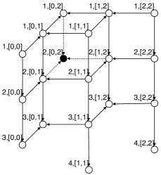
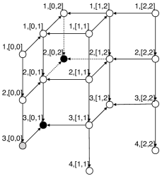
(a) $[0,2]$	(b) $[0,1]$	(c) $[0,0]$
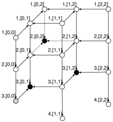
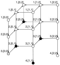
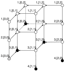
(d) $[1,2]$	(e) $[1,1]$	(f) $[2,2]$

Figure 4. Run-through example of the execution of Maximal-span-cores (Algorithm 4) over the search space of a temporal graph having $T=[0,2]$ (same as Figure 3(a)). Full nodes represent computed span-cores: span-cores in black are recognized as maximal, while those in gray are discarded from the set of the maximal span-cores.

6. Temporal community search

Community search in static graphs aims at finding a dense subgraph (community) containing a set of input query vertices (Fang et al., 2020; Huang et al., 2017). In the temporal setting it is very likely that the communities spanning the query vertices change over time. To be more precise, it may happen that a certain subgraph $S$ is a well-representative community for the given query vertices $Q$, but only for a certain time interval $\Delta$. Instead, for another time interval $\Delta^{\prime}$, a relevant community for $Q$ might correspond to a completely different subgraph $S^{\prime}$. For this reason, we formulate community search on temporal networks as the problem of finding $h$ subgraphs (with $h>0$ being an input parameter) containing the query vertices, together with their temporal span, such that the sum of the density of those subgraphs is maximized and the union of their temporal spans corresponds to the whole input temporal domain. Among the many densities proposed in the literature, here we follow the bulk of the literature on community search, and adopt the minimum-degree density (Fang et al., 2020; Huang et al., 2017). In fact, as well-discussed, among others, by Sozio and Gionis (Sozio and Gionis, 2010) in their seminal work, unlike other density notions, including the popular average degree, the minimum-degree density has the capability of mitigating the so-called “free-rider” effect, i.e., the fact that (large) subgraphs may be arbitrarily added to a community-search solution to artificially increase the objective-function value, and thus lead to unintuitive yet unnecessarily large output solutions. Formally, the problem we study in this work is:

Problem 3 (Temporal Community Search).

Given a temporal graph $G=(V,T,\tau)$, a set $Q\subseteq V$ of query vertices, and a positive integer $h\in\mathbb{N}^{+}$, find a set $\{\langle S_{i},\Delta_{i}\rangle\}_{i=1}^{h}$ of $h$ pairs such that ($i$) $\forall 1\leq i\leq h:Q\subseteq S_{i}\subseteq V$,  ($ii$) $\bigcup_{1\leq i\leq h}\Delta_{i}=T$,  and ($iii$) the following is maximized:

(1) $$\sum_{i=1}^{h}\min_{u\in S_{i}}\mbox{$d$}_{\Delta_{i}}(S_{i},u).$$

The input integer $h$ is a user-defined parameter that gives the analyst the flexibility of requiring a specific number of output temporal communities, which might vary from application to application.

6.1. Connection with Sequence Segmentation

Here we provide some theoretical insights into the Temporal Community Search problem. The main result we provide at the end of this subsection is an interesting connection with the well-established Sequence Segmentation problem (Bellman, 1961). As shown in the next subsections, such a result forms the basis for algorithmic design.

Let us first consider a single-interval variant of Problem 3: for a fixed temporal interval $\Delta$, find a subgraph containing the input set $Q$ of query vertices that maximizes the minimum temporal degree within $\Delta$. Formally:

Problem 4 (Single Temporal Community Search).

Given a temporal graph $G=(V,T,\tau)$, a set $Q\subseteq V$ of query vertices, and an interval $\Delta\sqsubseteq T$, find

$$S^{*}=\operatorname{argmax}_{Q\subseteq S\subseteq V}\min_{u\in S}\mbox{$d$}_{\Delta}(S,u).$$

It is easy to see that solving Problem 4 corresponds to solving minimum-degree-based community search on graph $G_{\Delta}$. Therefore, a solution to Problem 4 can straightforwardly be computed by applying a standard result on minimum-degree-based community search, which states that the highest-order core containing all query vertices is a solution to that problem (Barbieri et al., 2015). This finding is formalized next.

Definition 4 ($(Q,\Delta)$-highest-order-span-core).

Given a temporal graph $G=(V,T,\tau)$, a set $Q\subseteq V$ of query vertices, and an interval $\Delta\sqsubseteq T$, the $(Q,\Delta)$-highest-order-span-core of $G$, denoted $C^{*}_{Q,\Delta}$, is defined as the highest-order span-core among all span-cores of $G$ with temporal span $\Delta$ and containing all query vertices in $Q$. Let also $v^{*}_{Q,\Delta}$ denote the order of $C^{*}_{Q,\Delta}$.

Fact 1.

Given a temporal graph $G=(V,T,\tau)$, a set $Q\subseteq V$ of query vertices, and an interval $\Delta\sqsubseteq T$, the $(Q,\Delta)$-highest-order-span-core of $G$ is a solution to Problem 4 on input $\langle G,Q,\Delta\rangle$.

Note that Problem 4 may have multiple solutions: $C^{*}_{Q,\Delta}$ is only one of those possibly many ones. $C^{*}_{Q,\Delta}$ can be computed by running a core decomposition on (static) graph $G_{\Delta}$, and stopping it when the first core that does not contain all query vertices in $Q$ has been encountered. Therefore, Problem 4 can be solved in $\mathcal{O}(|\Delta|\times|E|)$ time.

In light of the above findings, an alternative yet equivalent way of formulating our Temporal Community Search problem is to ask for a segmentation (i.e., a partition) of the time domain $T$ into a set $\{\Delta_{i}\}_{i=1}^{h}$ of $h$ intervals so as to maximize the sum $\sum_{i=1}^{h}v^{*}_{Q,\Delta_{i}}$ of the orders of the $(Q,\Delta)$-highest-order-span-cores of those identified intervals. Once such an optimal segmentation of $T$ has been computed, the ultimate $\{\langle S_{i},\Delta_{i}\rangle\}_{i=1}^{h}$ pairs are derived by simply setting $S_{i}=C^{*}_{Q,\Delta_{i}}$, $\forall 1\leq i\leq h$. Formally:

Problem 5 (Alternative formulation of Problem 3).

Given a temporal graph $G=(V,T,\tau)$, a set $Q\subseteq V$ of query vertices, and a positive integer $h\in\mathbb{N}^{+}$, find a set $\{\langle S_{i},\Delta_{i}\rangle\}_{i=1}^{h}$ of $h$ pairs such that ($i$) $\forall 1\leq i\leq h:S_{i}=C^{*}_{Q,\Delta_{i}}$,  ($ii$) $\{\Delta_{i}\}_{i=1}^{h}$ is a partition of $T$,  and ($iii$) the following is maximized:

(2) $$\sum_{i=1}^{h}v^{*}_{Q,\Delta_{i}}.$$

Correspondence between Problem 3 and Problem 5 easily follows from Fact 1 and from the observation that for any feasible solution $\{\langle S_{i},\Delta_{i}\rangle\}_{i=1}^{h}$ to Problem 3 with overlapping intervals, there exists an overlapping-interval-free feasible solution with not smaller objective-function value. To see the latter, for any two overlapping intervals $\Delta_{i}$ and $\Delta_{j}$, simply replace one of the two intervals, say $\Delta_{i}$, with $\Delta^{\prime}_{i}=\Delta_{i}\setminus(\Delta_{i}\cap\Delta_{j})$. As $\Delta_{i}^{\prime}\sqsubseteq\Delta_{i}$, it holds that $v^{*}_{Q,\Delta^{\prime}_{i}}\geq v^{*}_{Q,\Delta_{i}}$, therefore the resulting overlapping-interval-free solution will have objective-function value greater than or equal to the objective-function value of the starting solution with overlapping intervals.

Thanks to the reformulation in Problem 5, it is immediate to observe that our Temporal Community Search problem is an instance of the well-established Sequence Segmentation problem, which asks for partitioning a sequence of numerical values into $b$ segments so as to minimize the sum of the penalties (according to some penalty function) on each identified segment (Bellman, 1961):

Problem 6 (Sequence Segmentation (Bellman, 1961)).

Given a sequence $X=(x_{0},x_{1},\ldots,x_{max})$ of numerical values, and a function $p:\{Y\}_{Y\sqsubseteq X}\rightarrow\mathbb{R}$ that assigns a penalty score to every subsequence $Y$ of $X$, partition $X$ into a set $\{X_{i}\}_{i=1}^{b}$ of $b$ subsequences such that $\sum_{i=1}^{b}p(X_{i})$ is minimized.

Fact 2.

Temporal Community Search (Problem 3) on input $\langle G=(V,T,\tau),Q,h\rangle$ is an instance of Sequence Segmentation (Problem 6) with $X=T$,  $b=h$,   and $\forall\Delta\sqsubseteq T:p(\Delta)=-v^{*}_{Q,\Delta}$.

In the following two subsections we show how to exploit the result in Fact 2 (and a further important finding about maximal span-cores) to design efficient algorithms for our Temporal Community Search problem.

1

Input: A temporal graph $G=(V,E,T)$, a set $Q\subseteq V$ of query vertices, an integer $h\in\mathbb{N}^{+}$.

Output: A set $\{\langle S_{i},\Delta_{i}\rangle\}_{i=1}^{h}$, where $Q\subseteq S_{i}\subseteq V$, $\forall 1\leq i\leq h$, and $\{\Delta_{i}\}_{i=1}^{h}$ is a partition of $T$.

2

/* Initialization */

3 Compute $v^{*}_{Q,\Delta}$ and $C^{*}_{Q,\Delta}$, $\forall\Delta\sqsubseteq T$, via $Q$-constrained span-core decomposition

$\mathbf{P}\leftarrow$ an empty $(|T|\times h)$-dimensional matrix

  // Penalty matrix

$\mathbf{R}\leftarrow$ an empty $(|T|\times h)$-dimensional matrix

  // Reconstruction matrix

4 forall $t\in T$ do

5       $\mathbf{P}[t,0]\leftarrow-v^{*}_{Q,[0,t]}$

6       $\mathbf{R}[t,0]\leftarrow 0$

7      

8

/* Dynamic-programming step */

9 forall $t\in T$ do

10       forall $i\in[1,h)$ do

11             $\mathbf{P}[t,i]\leftarrow\min_{\ell\in[0,t]}\mathbf{P}[\ell,i-1]-v^{*}_{Q,[\ell+1,t]}$

12             $\mathbf{R}[t,i]\leftarrow\operatorname{argmin}_{\ell\in[0,t]}\mathbf{P}[\ell,i-1]-v^{*}_{Q,[\ell+1,t]}$

13            

14      

15

/* Reconstruction of the solution */

16 $ub\leftarrow t_{max}$

17 forall $i\in(h,0]$ do

18       $lb\leftarrow\mathbf{R}[ub,i]$

19       $\Delta_{i}\leftarrow[lb,ub]$

20       $ub\leftarrow lb-1$

21      

22forall $i\in(h,0]$ do

23       $S_{i}\leftarrow C^{*}_{Q,\Delta_{i}}$

24

Algorithm 3 Temporal-community-search

6.2. A basic algorithm (based on all span-cores)

Sequence Segmentation can be solved in $\mathcal{O}(|X|^{2}\times h+\tau_{p})$ time via dynamic programming (Bellman, 1961), where $\tau_{p}$ is the overall time spent for computing the penalty score of all subsequences of the input sequence $X$ (according to the given penalty function $p$). Thanks to the connection shown in Fact 2, the dynamic-programming algorithm for Sequence Segmentation can be easily adapted to solve Temporal Community Search as well. The pseudocode of this algorithm – termed Temporal-community-search – is reported as Algorithm 3, and described next.

1

Input: A temporal graph $G=(V,E,T)$, a set $Q\subseteq V$ of query vertices, an integer $h\in\mathbb{N}^{+}$.

Output: A set $\{\langle S_{i},\Delta_{i}\rangle\}_{i=1}^{h}$, where $Q\subseteq S_{i}\subseteq V$, $\forall 1\leq i\leq h$, and $\{\Delta_{i}\}_{i=1}^{h}$ is a partition of $T$.

2

/* Identification of $T^{*}$ */

3

4Compute the set $\mathbf{C}_{M}(Q)$ of $Q$-constrained maximal span-cores of $G$

5 $\mathbf{D}\leftarrow\{\Delta\sqsubseteq T\mid C_{k,\Delta}\in\mathbf{C}_{M}(Q)\}$

6 $T_{\mathbf{D}}\leftarrow\bigcup_{\Delta\in\mathbf{D}}\Delta$;  $T_{\mathbf{D}}^{+}\leftarrow\{\min\{t_{e}\!+\!1,t_{max}\}\mid[t_{s},t_{e}]\in\mathbf{D}\}$;  $T_{\mathbf{D}}^{-}\leftarrow\{\max\{t_{s}\!-\!1,0\}\mid[t_{s},t_{e}]\in\mathbf{D}\}$

7 $T_{sup}\leftarrow\{t_{i}\in T\setminus(T_{\mathbf{D}}\cup T_{\mathbf{D}}^{-}\cup T_{\mathbf{D}}^{+}\cup\{t_{max}\})\mid i\in[1,h+1-|T_{\mathbf{D}}\cup T_{\mathbf{D}}^{-}\cup T_{\mathbf{D}}^{+}\cup\{t_{max}\}|]\}$

8 $T^{*}\leftarrow T_{\mathbf{D}}\ \cup\ T_{\mathbf{D}}^{+}\ \cup\ T_{\mathbf{D}}^{-}\ \cup\ \{t_{max}\}\ \cup\ T_{sup}$

9

/* Initialization */

10 Compute $v^{*}_{Q,\Delta}$, $\forall\Delta\sqsubseteq T$

11 $\mathbf{M}\leftarrow$ mapping function $[0,|T^{*}|)\rightarrow T^{*}$

$\mathbf{P}\leftarrow$ an empty $(|T^{*}|\times h)$-dimensional matrix

  // Penalty matrix

$\mathbf{R}\leftarrow$ an empty $(|T^{*}|\times h)$-dimensional matrix

  // Reconstruction matrix

12

13forall $r\in[0,|T^{*}|)$ do

14       $\mathbf{P}[r,0]\leftarrow-v^{*}_{Q,[0,\mathbf{M}[r]]}$

15       $\mathbf{R}[r,0]\leftarrow 0$

16      

17

/* Dynamic-programming step */

18 forall $r\in[0,|T^{*}|)$ do

19       forall $i\in[1,h)$ do

20             $\mathbf{P}[r,i]\leftarrow\min_{\ell\in[0,r]}\mathbf{P}[\ell,i-1]-v^{*}_{Q,[\mathbf{M}[\ell+1],\mathbf{M}[r]]}$

21             $\mathbf{R}[r,i]\leftarrow\operatorname{argmin}_{\ell\in[0,r]}\mathbf{P}[\ell,i-1]-v^{*}_{Q,[\mathbf{M}[\ell+1],\mathbf{M}[r]]}$

22            

23      

24

/* Reconstruction of the solution */

25 $ub\leftarrow|T^{*}|-1$

26 forall $i\in(h,0]$ do

27       $lb\leftarrow\mathbf{R}[ub,i]$

28       $\Delta_{i}\leftarrow[\mathbf{M}[lb],\mathbf{M}[ub]]$

29       $ub\leftarrow lb-1$

30      

31forall $i\in(h,0]$ do

32       $S_{i}\leftarrow C^{*}_{Q,\Delta_{i}}$

33

Algorithm 4 Efficient-temporal-community-search

The Temporal-community-search algorithm makes use of two $(|T|\times h)$-dimensional matrices, i.e., $\mathbf{P}$ and $\mathbf{R}$. Matrix $\mathbf{P}$ represents the penalty matrix. It contains, $\forall t\in T$, $\forall i\in[0,h)$, the minimum cost of segmenting the sequence corresponding to the first $t$ timestamps of $T$ into $i+1$ segments. As a result, $\mathbf{P}[t_{max},h-1]$ contains the objective-function value of the ultimate optimal solution to Problem 5. Matrix $\mathbf{R}$ is the reconstruction matrix. It provides information about the optimal segmentation, and is used at the end of the algorithm to reconstruct the output $\{\Delta_{i}\}_{i=1}^{h}$. Note that the algorithm does not explicitly compute the $S_{i}$ subgraphs corresponding to the optimal $\Delta_{i}$ intervals. In fact, as discussed above, each $S_{i}$ can be easily retrieved at the end of the algorithm, by simply setting it equal to the corresponding $(Q,\Delta_{i})$-highest-order-span-core $C^{*}_{Q,\Delta_{i}}$. According to Fact 2, the penalty score of an interval $\Delta\sqsubseteq T$ corresponds to $-v^{*}_{Q,\Delta}$, i.e., the negative of the order of the $(Q,\Delta)$-highest-order-span-core $C^{*}_{Q,\Delta}$. All individual $v^{*}_{Q,\Delta}$ values, for all $\Delta\sqsubseteq T$, are efficiently computed altogether, at the beginning of the algorithm, via a “$Q$-constrained” variant of span-core decomposition (an alternative, but much less efficient strategy consists in computing every single $v^{*}_{Q,\Delta}$ from scratch, on the fly). Specifically, a simple (yet more efficient) variant of the span-core decomposition algorithm (Algorithm 1) is employed for this purpose, which outputs only those span-cores containing all the vertices in $Q$. This is easily achievable by stopping the core-decomposition subroutine, for every interval $\Delta\sqsubseteq T$, as soon as a core not containing all query vertices in $Q$ has been encountered.

The time complexity of Algorithm 3 is $\mathcal{O}(|T|^{2}\times h+\tau_{sc})$, where $\tau_{sc}$ is the time spent for computing the $Q$-constrained span-core decomposition of the input graph $G$.

6.3. A more efficient algorithm (based on maximal span-cores)

A more efficient algorithm can be designed by noticing that, actually, one does not need to consider all timestamps in $T$ in the dynamic-programming step. Rather, focusing on a subset $T^{*}\subseteq T$ – which is properly defined based on the maximal span-cores of the input graph, see next – allows for significantly reducing the dimensionality of the penalty matrix $P$ and the reconstruction matrix $R$, hence the overall time complexity of the algorithm, without affecting optimality of the output solution. The following fact provides the theoretical basis for defining such a reduced temporal domain $T^{*}$.

Fact 3.

Given a temporal graph $G=(V,T,\tau)$ and a set $Q\subseteq V$ of query vertices, let $\mathbf{C}_{M}(Q)$ be the set of all $Q$-constrained maximal span-cores of $G$. For a temporal interval $\Delta\sqsubseteq T$, it holds that $v^{*}_{Q,\Delta}=\max\{0,\max\{k\mid C_{k,\Delta^{\prime}}\in\mathbf{C}_{M}(Q),\Delta\sqsubseteq\Delta^{\prime}\}\}$.

Fact 3 states that the penalty score $v^{*}_{Q,\Delta}$ of an interval $\Delta$ corresponds to the maximum among the orders of the $Q$-constrained maximal span-cores whose span includes $\Delta$, if some exist. If an interval $\Delta$ is not a subset of any span of a $Q$-constrained maximal span-core, then $v^{*}_{Q,\Delta}=0$. In that case, therefore, $\Delta$ can be safely discarded, as it cannot be part of the optimal solution of the given Temporal Community Search problem instance (unless it is needed to fill possible “holes”, see below). The ultimate consequence of this finding is that the aforementioned reduced temporal domain $T^{*}$ is identified by the timestamps covered by the spans of the maximal span-cores, along with auxiliary timestamps, which are needed to ensure a smooth execution of the dynamic-programming step, as well as a correct handling of some extreme cases. Specifically, let $\mathbf{D}=\{\Delta\sqsubseteq T\mid C_{k,\Delta}\in C_{M}(Q)\}$ be the set of the spans of the $Q$-constrained maximal span-cores of the input graph, and $T_{\mathbf{D}}=\bigcup_{\Delta\in\mathbf{D}}\Delta$ be the set of timestamps that are part of a span of a $Q$-constrained maximal span-core. The first two sets of auxiliary timestamps correspond to the timestamps that immediately precede and succeed the intervals in $\mathbf{D}$, i.e., the sets $T_{\mathbf{D}}^{+}=\{\min\{t_{e}+1,t_{max}\}\mid[t_{s},t_{e}]\in\mathbf{D}\}$ and $T_{\mathbf{D}}^{-}=\{\max\{t_{s}-1,0\}\mid[t_{s},t_{e}]\in\mathbf{D}\}$, respectively. The timestamps in $T_{\mathbf{D}}^{+}$ and $T_{\mathbf{D}}^{-}$ (along with the last timestamp $t_{max}$ of the input temporal domain $T$) are needed to allow the dynamic-programming step to identify a solution that actually covers the whole temporal domain $T$ (as per Condition ($ii$) of Problem 3). In particular, such timestamps may be interpreted as a trick to give the dynamic-programming step the flexibility to select “holes” (i.e., time intervals in-between two consecutive but not necessarily contiguous timestamps in $T_{\mathbf{D}}$). Moreover, we define $T_{sup}$ as the set of the first $h+1-|T_{\mathbf{D}}\cup T_{\mathbf{D}}^{-}\cup T_{\mathbf{D}}^{+}\cup\{t_{max}\}|$ timestamps of $T$ not contained in $T_{\mathbf{D}}\cup T_{\mathbf{D}}^{-}\cup T_{\mathbf{D}}^{+}\cup\{t_{max}\}$, i.e., $T_{sup}=\{t_{i}\in T\setminus(T_{\mathbf{D}}\cup T_{\mathbf{D}}^{-}\cup T_{\mathbf{D}}^{+}\cup\{t_{max}\})\mid i\in[1,h+1-|T_{\mathbf{D}}\cup T_{\mathbf{D}}^{-}\cup T_{\mathbf{D}}^{+}\cup\{t_{max}\}|]\}$. The timestamps in $T_{sup}$ are further auxiliary timestamps that are needed to return a correct $h$-sized solution when the timestamps in $T_{\mathbf{D}}\cup T_{\mathbf{D}}^{-}\cup T_{\mathbf{D}}^{+}\cup\{t_{max}\}$ are less than $h+1$ (the minimum number of timestamps required in $T^{*}$ to have a solution of size $h$). Note that $T_{sup}$ is nonempty only if $|T_{\mathbf{D}}\cup T_{\mathbf{D}}^{-}\cup T_{\mathbf{D}}^{+}\cup\{t_{max}\}|<h+1$. Ultimately, $T^{*}$ is defined as

$$T^{*}=T_{\mathbf{D}}\ \cup\ T_{\mathbf{D}}^{+}\ \cup\ T_{\mathbf{D}}^{-}\ \cup\ \{t_{max}\}\ \cup\ T_{sup}.$$

The proposed more efficient method for Temporal Community Search, termed Efficient-temporal-community-search, is summarized in Algorithm 4 and described next. The first five lines of the algorithm are devoted to the identification of $T^{*}$. As said above, matrices $\mathbf{P}$ and $\mathbf{R}$ have here reduced dimensionality with respect to Algorithm 3: they are $(|T^{*}|\times h)$-dimensional matrices, where $|T^{*}|\leq|T|$. A mapping function $\mathbf{M}$ is used to assign an index within $[0,|T^{*}|)$ to every timestamp in $|T^{*}|$ (Line 4). Such a mapping is needed to have every timestamp in $|T^{*}|$ logically assigned to a row of matrices $\mathbf{P}$ and $\mathbf{R}$. The rest of the algorithm resembles Algorithm 3, except for the fact that $\mathbf{M}$ is used every time that a row index has to be mapped to its corresponding timestamp (e.g., during the reconstruction of the solution).

An important point to clarify is that, during the execution of the Efficient-temporal-community-search algorithm, we might need the penalty score $v^{*}_{Q,\Delta}$ of intervals $\Delta\sqsubseteq T$ corresponding to non-maximal ($Q$-constrained) span-cores. Therefore, the algorithm needs the $v^{*}_{Q,\Delta}$ score of all intervals $\Delta\sqsubseteq T$. To compute these $v^{*}_{Q,\Delta}$ scores (and, related to this, the set $\mathbf{C}_{M}(Q)$ of $Q$-constrained maximal span-cores, at Line 4), there are two main options. The first one consists in computing the whole $Q$-constrained span-core decomposition (as done in Algorithm 3), keep the $v^{*}_{Q,\Delta}$ scores of all such cores, and eventually compute $\mathbf{C}_{M}(Q)$ by simply filtering out non-maximal span-cores. The second option corresponds instead to compute $\mathbf{C}_{M}(Q)$ directly, without passing through the whole $Q$-constrained span-core decomposition. This may be carried out by running a simple variant of the algorithm for computing maximal span-cores (Algorithm 2), where containment of query vertices is added as a further constraint. The computation of all the $v^{*}_{Q,\Delta}$ scores comes for free during the execution of this algorithm for $Q$-constrained maximal span-cores: these scores can therefore be retained by adding a few straightforward (constant-time) instructions to that algorithm. In our implementation we stick to the latter, as the Maximal-span-cores algorithm has been experimentally recognized as faster than the naïve filtering approach in all tested datasets.

The time complexity of the proposed Efficient-temporal-community-search algorithm is $\mathcal{O}(|T^{*}|^{2}\times h+\tau_{msc})$, with $\tau_{msc}$ being the time spent in computing the $Q$-constrained maximal span-cores and the penalty scores $v^{*}_{Q,\Delta}$. As in practice (attested by our experiments) $|T^{*}|\ll|T|$, the proposed Efficient-temporal-community-search algorithm is expected to be much more efficient than its naïve counterpart, i.e., Algorithm 3.

6.4. Minimum community search

An instance of Temporal Community Search may admit several optimal solutions which might differ either in terms of output intervals $\{\Delta_{i}\}_{i=1}^{h}$, or in terms of subgraphs assigned to the various identified intervals. More precisely, the latter refers to the fact that two optimal solutions might find the same segmentation $\{\Delta_{i}\}_{i=1}^{h}$ of the input temporal domain, but select different subgraphs $S_{i}$ for any interval $\Delta_{i}$. Therefore, if the communities $S_{i}$ are not chosen carefully, they may result to be excessively large, not really cohesive, and containing redundant/outlying vertices. This is a well-recognized issue of minimum-degree-based community search (Sozio and Gionis, 2010). At the same time, large communities might include more cohesive and denser subgraphs that still exhibit optimality. Motivated by this, in this subsection we devise a method to refine the communities originally found by our algorithms for Temporal Community Search, specifically attempting to minimize their size while preserving optimality. The main idea behind our refinement method is based on the following result:

Proposition 3 (Community containment).

Given a temporal graph $G=(V,T,\tau)$, a set $Q\subseteq V$ of query vertices, and a positive integer $h\in\mathbb{N}^{+}$, let $\{\langle S_{i},\Delta_{i}\rangle\}_{i=1}^{h}$ be a solution to Problem 3 on input $\langle G,Q,h\rangle$ with $S_{i}$ corresponding to the $(Q,\Delta_{i})$-highest-order-span-core of $G$, $\forall i\in[1,h]$. For every other solution $\{\langle S^{\prime}_{i},\Delta_{i}\rangle\}_{i=1}^{h}$ (referring to the same segmentation $\{\Delta_{i}\}_{i=1}^{h}$) to Problem 3 on input $\langle G,Q,h\rangle$ it holds that $S_{i}^{\prime}\subseteq S_{i}$, $\forall i\in[1,h]$.

Proof.

Let $k_{i}$ be the minimum degree of $S_{i}$, i.e., $k_{i}=v^{*}_{Q,\Delta_{i}}$ is the order of the $(Q,\Delta_{i})$-highest-order-span-core. Assume that there exists a solution $S^{\prime}_{i}$ to Problem 4 that is not contained in $S_{i}$. This implies that $(i)$ the minimum degree of a vertex of $S^{\prime}_{i}$ in $\Delta_{i}$ is $k_{i}$, and ($ii$) the minimum degree of a vertex of $S_{i}\cup S^{\prime}_{i}$ in $\Delta_{i}$ is $k_{i}$ as well. This violates the maximality condition of the definition of span-core, since, by hypothesis, $S_{i}$ corresponds to the $(Q,\Delta_{i})$-highest-order-span-core of $G$. ∎

The above proposition states that, given a solution $\{\langle S_{i},\Delta_{i}\rangle\}_{i=1}^{h}$ to the Temporal Community Search problem where every $S_{i}$ corresponds to the $(Q,\Delta_{i})$-highest-order-span-core of the input graph, one can focus on the various $S_{i}$ solely to refine the output communities, as such $S_{i}$ are guaranteed to contain all optimal solutions of the underlying problem instance (while keeping the segmentation $\{\Delta_{i}\}_{i=1}^{h}$ fixed). Within this view, we formulate the following optimization problem (which is a variant of Problem 4, with the additional constraint of requiring a smallest-sized solution):

Problem 7.

Given a temporal graph $G=(V,T,\tau)$, a set $Q\subseteq V$ of query vertices, and an interval $\Delta\sqsubseteq T$, let $S^{*}\subseteq V$ be the subset of vertices containing all the solutions to Problem 4 on input $\langle G,Q,\Delta\rangle$ (according to what stated in Proposition 3). Find

$$S^{*}_{min}={\operatorname{argmin}_{\{S\mid Q\subseteq S\subseteq S^{*},\min_{u\in S}\mbox{$d$}_{\Delta}(S,u)\geq\min_{u\in S^{*}}\mbox{$d$}_{\Delta}(S^{*},u)\}}|S|}.$$

Theorem 3.

Problem 7 in $\mathbf{NP}$-hard.

Proof.

Consider (the optimization version of) the $\mathbf{NP}$-hard mCST problem introduced by Cui et al. (Cui et al., 2014): given a graph $H=(V_{H},E_{H})$ and a query vertex $q\in V_{H}$, find a minimum-sized subgraph that contains $q$, is connected, and maximizes the minimum degree. Given an instance $\langle H,q\rangle$ of the mCST problem, construct an instance $\langle G,Q,\Delta\rangle$ of Problem 7 by defining $G$ as composed by a single temporal snapshot corresponding to graph $H$, $\Delta$ as a singleton interval composed of the single timestamp of $G$, and setting $Q=\{q\}$. It is straightforward to see that solving Problem 7 on input $\langle G,Q,\Delta\rangle$ is equivalent to solving mCST on input $\langle H,q\rangle$, as the constraint about connectedness is automatically satisfied in Problem 7 for the special case of a single query vertex. ∎

1

Input: A temporal graph $G=(V,E,T)$, a set $Q\subseteq V$ of query vertices, an interval $\Delta\sqsubseteq T$, a subset of vertices $S^{*}\subseteq V$ containing all the solutions to Problem 4 on input $\langle G,Q,\Delta\rangle$.

Output: A subset $S^{*}_{min}$ of vertices such that $Q\subseteq S^{*}_{min}\subseteq S^{*}$ and $\min_{u\in S^{*}_{min}}\mbox{$d$}_{\Delta}(S^{*}_{min},u)\geq\min_{u\in S^{*}}\mbox{$d$}_{\Delta}(S^{*},u)$.

2

3$S^{*}_{min}\leftarrow\emptyset$;   $P\leftarrow\emptyset$;   $\mathcal{A}\leftarrow\emptyset$

4 add every $q\in Q$ to $P$ with priority $+\infty$

5 $k^{*}\leftarrow\min_{u\in S^{*}}\mbox{$d$}_{\Delta}(S^{*},u)$;   $k^{*}_{min}\leftarrow 0$

6

7while $k^{*}_{min}<k^{*}$ or $Q\not\subseteq S^{*}_{min}$ do

8       dequeue $u$ from $P$

9       $S^{*}_{min}\leftarrow S^{*}_{min}\cup\{u\}$

10      

11      forall $v\in neigh_{\Delta}(S^{*},u)\setminus S^{*}_{min}\setminus P$ do

12             $\mathcal{A}[v]\leftarrow score(v)$

13             add $v$ to $P$ with priority $\mathcal{A}[v]$

14      

15      forall $v\in neigh_{\Delta}(S^{*}_{min},u)$ do

16            

17            if $\mbox{$d$}_{\Delta}(S^{*}_{min},v)=k^{*}$ then

18                   forall $w\in neigh_{\Delta}(P,v)$ do

19                         $\mathcal{A}[w]\leftarrow\mathcal{A}[w]-1$

20                        

21                  

22            

23      $k^{*}_{min}\leftarrow\min_{v\in S^{*}_{min}}\mbox{$d$}_{\Delta}(S^{*}_{min},v)$

24      

Algorithm 5 Greedy-minimum-community-search

As Problem 7 is $\mathbf{NP}$-hard, we devise a heuristic that is inspired to the greedy one proposed for the Minimum Community Search problem in (Barbieri et al., 2015). The proposed heuristic is outlined in Algorithm 5 and described next. In the pseudocode and in the following we denote as $k^{*}$ and $k^{*}_{min}$ the minimum degree of $S^{*}$ and $S^{*}_{min}$, respectively, and as $neigh_{\Delta}(S,u)$ the neighbors of a vertex $u\in V$ in the subgraph induced by $S\subseteq V$ and $\Delta\sqsubseteq T$. Algorithm 5 iteratively adds vertices to the solution $S^{*}_{min}$ according to a priority queue $P$. Priorities of vertices in $P$ are defined based on a score that measures how promising a vertex is for making the current solution $S^{*}_{min}$ reach the optimal minimum degree. Specifically, the score of a vertex $u\in S^{*}$ is defined as:

$$score(u)=score^{+}(u)-score^{-}(u),$$

where

$$score^{+}(u)=|\{v\in neigh_{\Delta}(S^{*}_{min},u)\mid\mbox{$d$}_{\Delta}(S^{*}_{min},v)<k^{*}\}|;$$

$$score^{-}(u)=\max\{0,k^{*}-\mbox{$d$}_{\Delta}(S^{*}_{min},u)\}.$$

$score^{+}(u)$ is the gain effect of adding $u$ to $S^{*}_{min}$, while $score^{-}(u)$ is the penalty effect. In particular, $score^{+}(u)$ counts the number of neighbors of $u$ in $S^{*}_{min}$ that would benefit from the inclusion of $u$ to $S^{*}_{min}$, i.e., that have degree less than $k^{*}$. On the other hand, $score^{-}(u)$ represents the number of neighbors of $u$ still required in $S^{*}_{min}$ so that $u$ has degree at least $k^{*}$. The algorithm starts by adding the query vertices to the queue $P$ with priority $+\infty$, in order to ensure that they will be selected at the very beginning. At each iteration of the main cycle of the algorithm (starting at Line 5), the vertex $u$ exhibiting the highest priority is dequeued from $P$ and is added to the solution $S^{*}_{min}$. As a consequence, a couple of updates are performed. First, $u$’s neighbors not in the priority queue $P$ are added to it (Lines 5-5). Note that this is the only step of the algorithm where the score of a vertex is computed from scratch and stored in $\mathcal{A}$, a map that keeps the scores of all vertices in $P$ up-to-date during the whole execution of the algorithm. The second update consists in recomputing the score of every $v$’s neighbor $w$ in the queue, if a vertex $v\in S^{*}_{min}$ has reached the desired minimum degree $k^{*}$ after the addition of $u$.

7. Experiments

Table 1. Temporal graphs used in the experiments.

dataset	$|V|$	$|E|$	$|T|$	window size	domain
HighSchool	$327$	$47$k	$1212$	$5$ mins	face-to-face
PrimarySchool	$242$	$55$k	$390$	$5$ mins	face-to-face
HongKong	$806$	$2$M	$2976$	$5$ mins	face-to-face
ProsperLoans	$89$k	$3$M	$307$	$7$ days	economic
Last.fm	$992$	$4$M	$77$	$21$ days	co-listening
WikiTalk	$2$M	$10$M	$192$	$28$ days	communication
DBLP	$1$M	$11$M	$80$	$366$ days	co-authorship
StackOverflow	$2$M	$16$M	$51$	$56$ days	question answering
Wikipedia	$343$k	$18$M	$101$	$56$ days	co-editing
Amazon	$2$M	$22$M	$115$	$28$ days	co-rating
Epinions	$120$k	$33$M	$25$	$21$ days	co-rating

Table 2. Evaluation of the proposed algorithms: number of output span-cores, running time, memory, and number of processed vertices.

		# output	running	memory	# processed
dataset	method	span-cores	time (s)	(GB)	vertices
HighSchool	Naïve-span-cores	$12\,320$	$18$	$0.1$	$3$M
	Span-cores		$1$	$0.1$	$581$k
	Naïve-maximal-span-cores	$450$	$1$	$0.1$	$581$k
	Maximal-span-cores		$0.3$	$0.1$	$181$k
PrimarySchool	Naïve-span-cores	$4\,703$	$4$	$0.1$	$818$k
	Span-cores		$0.6$	$0.1$	$174$k
	Naïve-maximal-span-cores	$409$	$0.6$	$0.1$	$174$k
	Maximal-span-cores		$0.1$	$0.1$	$63$k
HongKong	Naïve-span-cores	$2\,367\,743$	$85\,180$	$1$	$819$M
	Span-cores		$18\,389$	$0.8$	$216$M
	Naïve-maximal-span-cores	$1\,807$	$18\,641$	$0.8$	$216$M
	Maximal-span-cores		$339$	$0.5$	$212$M
ProsperLoans	Naïve-span-cores	$4\,273$	$101$	$2$	$55$M
	Span-cores		$46$	$2$	$27$M
	Naïve-maximal-span-cores	$293$	$48$	$2$	$27$M
	Maximal-span-cores		$8$	$2$	$980$k
Last.fm	Naïve-span-cores	$126\,819$	$707$	$0.5$	$2$M
	Span-cores		$199$	$0.5$	$531$k
	Naïve-maximal-span-cores	$1\,670$	$202$	$0.5$	$531$k
	Maximal-span-cores		$57$	$0.5$	$271$k
WikiTalk	Naïve-span-cores	$19\,693$	$322\,302$	$36$	$25$B
	Span-cores		$1\,084$	$36$	$555$M
	Naïve-maximal-span-cores	$632$	$1\,194$	$36$	$555$M
	Maximal-span-cores		$126$	$35$	$2$M
DBLP	Naïve-span-cores	$6\,135$	$10\,506$	$11$	$1$B
	Span-cores		$278$	$11$	$150$M
	Naïve-maximal-span-cores	$268$	$292$	$11$	$150$M
	Maximal-span-cores		$116$	$11$	$620$k
StackOverflow	Naïve-span-cores	$1\,238$	$5\,360$	$10$	$1$B
	Span-cores		$245$	$10$	$127$M
	Naïve-maximal-span-cores	$129$	$245$	$10$	$127$M
	Maximal-span-cores		$128$	$10$	$3$M
Wikipedia	Naïve-span-cores	$125\,191$	$17\,155$	$4$	$1$B
	Span-cores		$522$	$4$	$35$M
	Naïve-maximal-span-cores	$2\,147$	$537$	$4$	$35$M
	Maximal-span-cores		$201$	$4$	$320$k
Amazon	Naïve-span-cores	$29\,318$	$10\,415$	$18$	$2$B
	Span-cores		$409$	$18$	$247$M
	Naïve-maximal-span-cores	$303$	$580$	$18$	$247$M
	Maximal-span-cores		$123$	$18$	$688$k
Epinions	Naïve-span-cores	$63\,111$	$699$	$4$	$39$M
	Span-cores		$186$	$4$	$3$M
	Naïve-maximal-span-cores	$320$	$201$	$4$	$3$M
	Maximal-span-cores		$154$	$5$	$129$k

In this section we present an experimental evaluation to empirically assess the performance of all the proposed methods. Specifically, we focus on whole span-core decomposition (Section 7.1), maximal span-cores (Section 7.2), characterization of the extracted span-cores (Section 7.3), and temporal community search (Section 7.5).

Datasets. We use eleven real-world datasets recording timestamped interactions between entities. For each dataset we select a window size to define a discrete time domain, composed of contiguous timestamps of the same duration, and build the corresponding temporal graph. If multiple interactions occur between two entities during the same discrete timestamp, they are counted as one. The characteristics of the resulting temporal graphs, along with the selected window sizes, are reported in Table 1.

The three smallest datasets were gathered by using wearable proximity sensors in schools, with a temporal resolution of $20$ seconds. PrimarySchool contains the contact events between $242$ volunteers ($232$ children and $10$ teachers) in a primary school in Lyon, France, during two days (Stehlé et al., 2011). HighSchool${}^{\ref{foot:school}}$ describes the close-range proximity interactions between students and teachers ($327$ individuals overall) of nine classes during five days in a high school in Marseilles, France (Mastrandrea et al., 2015). HongKong reports the same kind of interactions for a primary school in Hong Kong, whose population consists of $709$ children and $65$ teachers divided into thirty classes, for eleven consecutive days (Sapienza et al., 2015).

ProsperLoans represents the network of loans between the users of Prosper, a marketplace of loans between privates. Last.fm${}^{\ref{foot:konect}}$ records the co-listening activity of the Last.fm streaming platform: an edge exists between two users if they listened to songs of the same band within the same discrete timestamp. WikiTalk${}^{\ref{foot:konect}}$ is the communication network of the English Wikipedia. DBLP${}^{\ref{foot:konect}}$ is the co-authorship network of the authors of scientific papers from the DBLP computer science bibliography. StackOverflow includes the answer-to-question interactions on the stack exchange of the stackoverflow.com website. Wikipedia${}^{\ref{foot:konect}}$ connects users of the Italian Wikipedia that co-edited a page during the same discrete timestamp. Finally, for both Amazon${}^{\ref{foot:konect}}$ and Epinions${}^{\ref{foot:konect}}$, vertices are users and edges represent the rating of at least one common item within the same discrete timestamp.

Implementation. All methods are implemented in Python (v. 2.7.16) and compiled by Cython. All the experiments were run on a machine equipped with Intel Xeon CPU at 2.1GHz. The experiments reported in Sections 7.1 and 7.2 used 64GB RAM, while the ones in Section 7.5 used 32GB RAM.

7.1. Span-core decomposition

We compare the two methods to compute a complete decomposition described in Section 4, i.e., the baseline Naïve-span-cores and the proposed Span-cores, in terms of execution time, memory, and total number of vertices input to the core-decomposition subroutine. We report these measures, together with the number of span-cores and maximal span-cores of each dataset, in Table 2.

In terms of execution time, Span-cores considerably outperforms Naïve-span-cores in all datasets, achieving a speed-up from $2.1$ up to two orders of magnitude. The speed-up is explained by the number of vertices processed by the core-decomposition subroutine, which is the most time-consuming step of the algorithms albeit linear in the size of the input subgraph. The difference of this quantity between Span-cores and Naïve-span-cores reaches over an order of magnitude in the WikiTalk, Wikipedia, and Epinions dataset, confirming the effectiveness of the “horizontal containment” relationships. The memory required by the two procedures is comparable in all cases since the largest structures needed in memory are the temporal graph itself and the set $\mathbf{C}$ of all span-cores.

7.2. Maximal span-cores

We compare our Maximal-span-cores algorithm to the naïve approach, described at the beginning of Section 5, based on running the Span-cores algorithm and filtering out the non-maximal span-cores, which we refer to as Naïve-maximal-span-cores. The results are again reported in Table 2.

Naïve-maximal-span-cores behaves very similarly to Span-cores: they only differ for the filtering mechanism which requires a few additional seconds in most cases. Maximal-span-cores is much faster than Naïve-maximal-span-cores for all datasets, with a speed-up from $1.3$ for the Epinions dataset to one order of magnitude for the HongKong dataset. Except for the school datasets and Last.fm, the difference in terms of number of processed vertices is between one and three orders of magnitude, attesting the advantages of the top-down strategy of Maximal-span-cores, which avoids the visit of portions of the span-core search space and handles the overhead of reconstructing graphs, i.e., $(V_{lb},E_{\Delta}[V_{lb}])$, efficiently. Finally, the memory requirements of the two methods are comparable for all datasets.

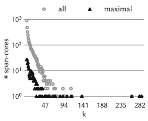
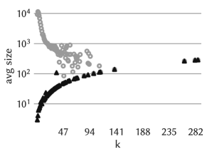
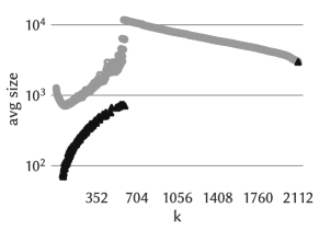
DBLP Epinions

Figure 5. Top plots: number of span-cores and maximal span-cores as a function of the order $k$. Bottom plots: average size of all span-cores and maximal span-cores as a function of the order $k$.

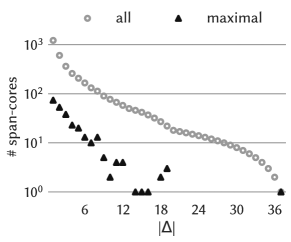
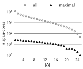
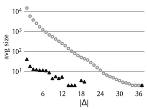
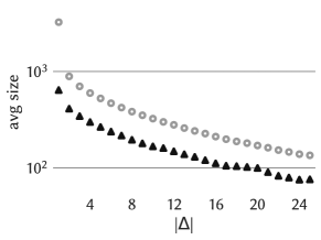
DBLP Epinions

Figure 6. Top plots: number of span-cores and maximal span-cores as a function of the size of the temporal span $|\Delta|$. Bottom plots: average size of all span-cores and maximal span-cores as a function of the size of the temporal span $|\Delta|$.

7.3. Span-cores characterization

We compare and characterize all span-cores against maximal span-cores. At first, Table 2 shows that span-cores are at least one order of magnitude more numerous than maximal span-cores for all datasets, with the maximum difference of three orders of magnitude for the HongKong dataset.

In Figure 5 we show the number (top) and the average size (bottom) of span-cores and maximal span-cores as a function of the order $k$ for the DBLP and Epinions datasets. For both datasets, the number of maximal span-cores is at least one order of magnitude lower than the total number of span-cores up to a quarter of the $k$ domain, where the span-cores are more numerous. Instead, in the rest of the domain, they mostly coincide due to the maximality condition over $|\Delta|$. The average size is also smaller for maximal span-cores, difference that wears thin when the gap between the numbers of span-cores and maximal span-cores starts decreasing since, for high values of $k$, most (or all) span-cores are maximal.

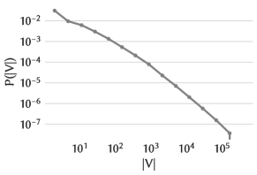
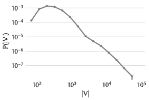
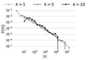
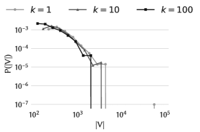
DBLP Epinions

Figure 7. Distribution of sizes of the span-cores. Top plots: overall distributions. Middle plots: distributions of the sizes of span-cores with fixed temporal span. Bottom plots: distributions of the sizes of span-cores with fixed order.

Figure 6 shows a different picture when numbers and average sizes of span-cores are shown as a function of the size of the span $|\Delta|$. For both datasets, the number of span-cores and maximal span-cores is decreasing – which is expected since the number of intervals decreases when $|\Delta|$ increases – with a constant gap close to one and two orders of magnitude, respectively. On the other hand, the behavior of the average size is quite different between the two datasets. For low values of $|\Delta|$, the average size of span-cores of the DBLP dataset is much higher than the average size of maximal span-cores, then the difference decreases and vanishes at the end of domain where a maximal span-core of $|\Delta|=37$ dominates all other span-cores with $|\Delta|\geq 20$. Instead, for the Epinions dataset, the average size of all span-cores and of maximal span-cores follow the same behavior, with a difference of less than an order of magnitude, because the maximality condition over $k$ excludes the largest span-cores from the set of maximal span-cores.

Figure 7 yields some additional insights by showing the whole distribution of sizes of the span-cores: these distributions are very skewed and span several orders of magnitude. The figure also shows the size distributions of span-cores with a given order or duration: all are broad, becoming narrower as the order or duration increase. We have also considered randomized versions of the datasets, in which edges are reshuffled at random at each timestamp. In this case as well, the distributions of the sizes of the span-cores are found to be broad, showing that the heterogeneity in span-core sizes can also be obtained in largely random data. However, the cohesive temporal structures are destroyed in the reshuffled data (see also Section 8.1): all the span-cores have then very small order and span.

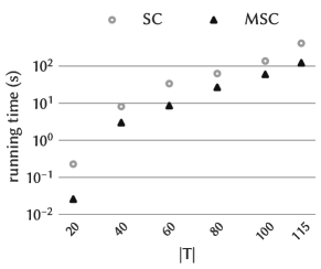
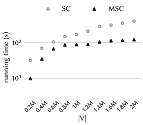
Figure 8. Scalability analysis: running time of the algorithms for extracting all the span-cores (SC, Algorithm 1) and only the maximal span-cores (MSC, Algorithm 2) as a function of the number timestamps and vertices, on the Amazon dataset.

7.4. Scalability analysis

Here we evaluate the scalability of Algorithms 1 and 2. To this aim, we consider temporal subgraphs derived from the Amazon dataset with increasing number of vertices and timestamps. To obtain temporal subgraphs with varying number of timestamps, we simply consider the temporal graphs associated with the first $20$, $40$, $60$, $80$, $100$ timestamps, while considering all the vertices and edges existing in these time-frames. For what concerns the temporal subgraphs with controlled number of vertices, we consider the entire temporal domain and sample sets of vertices of size $0.2M$, $0.4M$, $0.6M$, $0.8M$, $1M$, $1.2M$, $1.4M$, $1.6M$, $1.8M$. Vertices are sampled according to the following simple procedure:

• Select a vertex uniformly at random from the whole $V$ and add such a vertex to the set of sampled nodes $S$

• Starting from the first timestamp of the temporal domain $T$, iteratively

  • For each vertex $v$ in $S$ select a neighbor of $v$ uniformly at random and add it to $S$

  • Move to the next timestamp

• If the last timestamp is reached, restart from the first one

The results of this scalability experiment are reported in Figure 8. It can be observed that the trends shown in the figure comply with the time complexities discussed in Sections 4–5: running times are quadratic in the number of timestamps and linear in the number of vertices/edges. Another relevant consideration is that the difference between the algorithm to compute maximal span-cores and the one for computing all the span-cores gets larger as the number of timestamps or vertices increase. This further attests the usefulness of introducing an algorithm that is specifically devoted to maximal-span-core computation.

7.5. Temporal community search

In this subsection we assess the performance of the proposed algorithms for temporal community search (presented in Sections 6.2–6.3), as well as the greedy procedure for reducing the size of the output communities (presented in Section 6.4). In the remainder of this subsection we refer to our basic algorithm (i.e., Algorithm 3, which precomputes the penalty scores via span-core decomposition) as SC-TCS, and to our more efficient algorithm (i.e., Algorithm 4, which exploits maximal span-cores to reduce the number of timestamps to be considered) as MSC-TCS. We also involve in the comparison a naïve version of Algorithm 3, where the penalty scores of the various intervals are computed from scratch during the execution of the algorithm, instead of precomputing them all via span-core decomposition. We refer to such a naïve method as Naïve-TCS.

The experimental setting we consider here is as follows. We vary the number $|Q|$ of query vertices from 1 to 3. In particular, when $|Q|=1$, we sample the single query vertex uniformly at random from the whole vertex set $V$. Instead, for $|Q|>1$, we employ a more sophisticated sampling strategy that aims at finding meaningful query-vertex sets, i.e., vertices interacting with each other during the temporal observations, and, at the same time, independent from the specific form of the resulting span-core decomposition. Specifically, the sampling strategy we use is based on an adaptation of random walk to the temporal settings:

• Select a vertex uniformly at random from the whole $V$ and add such a vertex to the set $Q_{\operatorname*{visited}}$ of visited vertices

• Starting from the first timestamp of the temporal domain $T$, iteratively:

  • With probability $p$, move the random walker to a neighbor of the current vertex and add the neighbor to $Q_{\operatorname*{visited}}$. If the current vertex has no neighbors in a given timestamp, the random walker jumps to the first next timestamp in which that vertex has at least one neighbor

  • With probability $1-p$, keep the random walker at the current vertex, but go to the next timestamp

• Restart if the last timestamp of $T$ is reached

• Stop when $|Q_{\operatorname*{visited}}|$ reaches a proper (user-defined) size $\nu$

• Sample $|Q|$ query vertices from $Q_{\operatorname*{visited}}$ with probability proportional to the frequency of the visits during the random walk

In our experiments we set $p=0.8$ and $\nu=3|Q|$. As far as the number $h$ of output communities, we consider the range $h\in[10,20,30,40,50,60]$ on all datasets, with the exception of StackOverflow, for which we discard $h=60$, and Epinions, for which we consider $h\in[4,8,12,16,20,24]$. For every parameter configuration, we perform five runs of every algorithm (in every run we sample a different query-vertex set). Note that we were not able to run the algorithms for temporal community search on the WikiTalk dataset due to memory constraints.

Running time. In Figure 9 we show the running time of the proposed algorithms as a function of the number $h$ of output communities, for the HighSchool, DBLP, Wikipedia, and Amazon datasets. The first general observation we make is that the running time of all algorithms increases as $h$ gets higher. This in accordance with the time-complexity analysis reported in Section 6. Also, running times are independent of the selected query-vertex set $Q$. Looking at the individual performance, we notice that, as expected, the Naïve-TCS method has severe limitations in terms of efficiency: it takes hours to run on the HighSchool and Wikipedia datasets, while it is not able to terminate in less than 10 days on the remaining datasets. SC-TCS and MSC-TCS are much faster than Naïve-TCS, achieving a speedup of up to more than four orders of magnitude. MSC-TCS is in most cases faster than SC-TCS, with speedup up to one order of magnitude (on HighSchool, for $h=60$). This confirms that the exploitation of the maximal span-cores is effective in both shortening the precomputation time and reducing the temporal domain considered in the dynamic-programming step. The only exception is the Wikipedia dataset. To dive deeper into the motivations of this exception, we report in Figure 10 the split of the average running time of SC-TCS and MSC-TCS into the time spent in the dynamic-programming step (DP) (which also includes the identification of the reduced temporal domain $T^{*}$ for MSC-TCS), and the precomputation time (i.e., the time required for computing all penalty scores via span-core decomposition or maximal span-cores). Interestingly, what affects the most the running time is the precomputation of the scores. Apparently, the $Q$-constrained version of Span-cores is more efficient than Maximal-span-cores in some datasets, which we believe is due to the structure of the search space. On the other hand, these results confirm that the reduction of the temporal domain considered by the dynamic-programming step is actually effective since the DP running time of MSC-TCS is always less than (or equal to) the DP running time of SC-TCS.

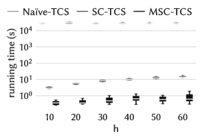
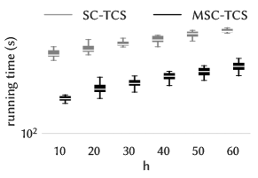
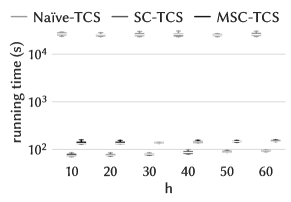
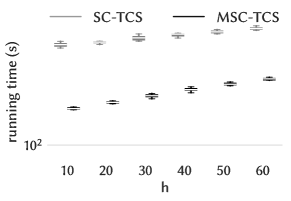
HighSchool DBLP Wikipedia Amazon

Figure 9. Running time of the algorithms for Temporal Community Search, as a function of the number $h$ of output communities. Each boxplot corresponds to 15 data points.

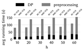
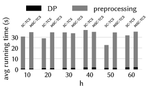
Wikipedia Last.fm

Figure 10. Split of the average running time of the SC-TCS and MSC-TCS algorithms into dynamic programming (DP) and precomputation, for the Wikipedia and Last.fm datasets.

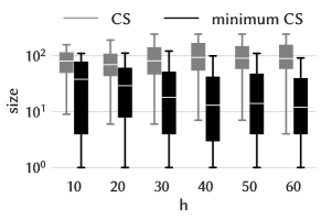
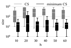
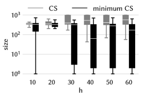
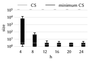
PrimarySchool HongKong Last.fm Epinions

Figure 11. Comparison of the size of the communities in the solutions to Temporal Community Search: original output of the algorithms for Temporal Community Search (CS) and after running the Greedy-minimum-community-search algorithm on top of them (minimum CS). Each boxplot corresponds to 15 data points.

Greedy-minimum-community-search. Here we evaluate the performance of the proposed Greedy-minimum-community-search algorithm (Algorithm 5) for reducing the size of the output communities. We recall that the proposed algorithms for Temporal Community Search (evaluated above) output communities corresponding to the $(Q,\Delta_{i})$-highest-order-span-cores for all $\{\Delta_{i}\}_{i=1}^{h}$ temporal intervals identified. The Greedy-minimum-community-search algorithm takes every $(Q,\Delta_{i})$-highest-order-span-core and attempts to reduce its size, while preserving optimality. Thus, the ultimate goal of the evaluation presented next is to show how well Greedy-minimum-community-search is able to reduce the size of the original span-cores, and what is its overhead in terms of running time.

Figure 11 compares the size of the starting $(Q,\Delta_{i})$-highest-order-span-cores and the size of the corresponding reduced community yielded by the Greedy-minimum-community-search algorithm, for the PrimarySchool, HongKong, Last.fm, and Epinions datasets. It can be easily observed that, as a general trend, the reduced communities are much smaller than the original ones, in all datasets, up to four orders of magnitude. The results on the Epinions dataset are a bit different than the other three datasets. In fact, on that dataset, the original communities (CS) always include the whole $120$k vertices of the graph, while the communities found by Greedy-minimum-community-search (minimum CS) have median size smaller than $10$, and, in many cases, they correspond to communities composed of the query vertices only. This means that, on the Epinions dataset, for our tested queries, the algorithms for Temporal Community Search do not extract communities that are really cohesive around the query vertices. This way, the benefits of exploiting an a-posteriori community-size-reduction step are less evident. Also, we do not notice any evident pattern as a function of $h$, for any dataset.

In Table 3 we report the average running time of an execution of Greedy-minimum-community-search, for all datasets. Note that this is the average time required to process one of the $h$ communities in a solution to Temporal Community Search. Greedy-minimum-community-search runs in $8$ seconds or less in all tested datasets. Therefore, the additional running time required by the algorithm is rather negligible.

To summarize, Greedy-minimum-community-search is empirically recognized as a powerful post-processing method for improving the quality of the solutions to Temporal Community Search: it finds much smaller communities at a very small additional computational cost.

Table 3. Average running time of an execution of the Greedy-minimum-community-search algorithm.

	HighSchool	PrimarySchool	HongKong	ProsperLoans	Last.fm
running time (s)	$0.003$	$0.001$	$0.02$	$0.3$	$0.06$

	DBLP	StackOverflow	Wikipedia	Amazon	Epinions
running time (s)	$7$	$8$	$1$	$7$	$6$

8. Applications

In this section we illustrate applications of (maximal) span-cores in the analysis of face-to-face interaction networks, and how the methods for Temporal Community Search can be profitably exploited in a task of graph classification. For these applications we use the three networks gathered in schools, i.e., PrimarySchool, HighSchool, and HongKong, which are described above, at the beginning of Section 7. We use a window size of $5$ minutes and, in the analysis, we discard span-cores of $|\Delta|=1$, i.e., having span of $5$ minutes, since they represent short interactions, not significant for our purposes. In the following we show ($i$) three types of interesting temporal patterns (Section 8.1), i.e., social activities of groups of students within a school day, mixing of gender and class, and length of social interactions in groups; ($ii$) a procedure to detect anomalous contacts and intervals that exploits maximal span-cores (Section 8.2); and, ($iii$) an approach to graph classification based on temporal community search (Section 8.3).

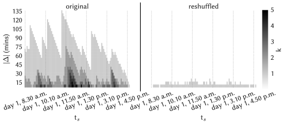
PrimarySchool

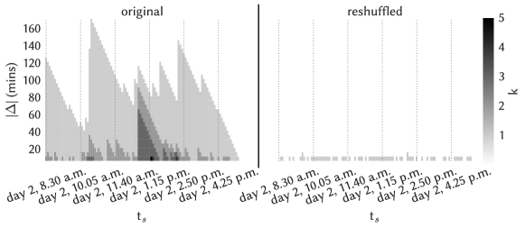
HighSchool

Figure 12. Temporal activity of a school day of the PrimarySchool and HighSchool datasets: the $x$ axis reports the hour of the day at which the span of a span-core starts, the $y$ axis specifies the size of the span (in minutes), and the color scale shows the order $k$. At a glance, it can be observed that the temporal structure of the span-core decomposition detects time-evolving cohesive structures in the original datasets (left plots) that completely disappear in the reshuffled datasets (right plots).

8.1. Temporal patterns

Temporal activity. We first show how span-cores afford a simple temporal analysis of social activities of groups of people within a school day. The left side of Figure 12 reports colormaps of the order $k$ of the span-cores as a function of their starting time $t_{s}$ ($x$ axis) and of the size of their temporal span $|\Delta|$ ($y$ axis), for a school day of the PrimarySchool and HighSchool datasets. Darker gray indicates span-cores of high order and slots located in the upper part of the plots refer to span-cores of long span. It is important to notice that the linear decay in span duration is naturally due to the definition of span-core and to the shifting of the starting time $t_{s}$; therefore, it is not a distinguishing feature of the activity patterns found in the analyzed data. In both datasets, fluctuations of $k$ and $|\Delta|$ are observed along the day, which can be related to school events. Around $10$ a.m., the size of the span $|\Delta|$ reaches a local maximum in correspondence to the morning break, which means that students establish long-lasting interactions that hold beyond the break itself. Moreover, when classes gather for the lunch break, the order $k$ reaches its maximum value since students tend to form larger and more cohesive groups.

In order to verify that these results are not trivially derived from the general temporal activity, as simply given by the number of interactions in each timestamp, we compare our findings to a null model. At each timestamp of the temporal graphs, we reshuffle the edges by the Maslov-Sneppen algorithm (Maslov and Sneppen, 2002) which consists in repeating the following operations up to when all edges have been processed: select at random two edges with no common vertices, e.g., $(u,v)$ and $(w,z)$, and transform them into $(u,z)$ and $(w,v)$, if neither $(u,z)$ and $(w,v)$ existed in the original timestamp. This reshuffling preserves the degree of each vertex in each timestamp and the global activity (i.e., the number of contacts per timestamp), but destroys correlations between edges of successive timestamps. In the right side of Figure 12 we show the results of the temporal analysis described above for the reshuffled datasets. In both, the values of $|\Delta|$ and $k$ reached are much smaller than in the original datasets. The size of the span $|\Delta|$ is always shorter than $20$ minutes, while in the original datasets it is much longer, up to $170$ minutes, and the order $k$ is always equal to $1$, compared to the original maximum of $5$. The time-evolving cohesive structures detected by the temporal core decomposition in the original datasets are completely lost on reshuffling, since only span-cores of short span and low coreness are observed in the latter case. This shows that the temporal structure exposed by the span-core decomposition is not simply a consequence of temporal patterns of global activity but that span-cores represent a concrete method to detect complex cohesive structures and their temporal evolution.

Mixing patterns. We now show an analysis of mixing patterns of students with respect to gender and class. Such vertex attributes are indeed available for the individuals of the PrimarySchool dataset. We define as gender purity of a span-core the fraction of individuals of the most represented gender within the span-core. Class purity is analogously defined. The left plot of Figure 13 reports the temporal evolution of the average gender and class purity of the maximal span-cores spanning each timestamp, during the first school day of the PrimarySchool dataset. During lessons, when students are in their own classes, class purity has naturally very high values, very close to $1$. Gender purity is instead rather low. On the other hand, when students are gathered together, during the morning break at $10$ a.m. and the lunch break between $12$ a.m. and $2$ p.m., the situation is overturned: gender purity reaches large values while class purity drastically decreases. This shows that primary school students group with individuals of the same class, disregarding the gender, only when they are forced by the schedule of the lessons, but prefer on average to form cohesive groups with students of the same gender during breaks. This is in agreement and complements a previous study of the same dataset focusing on single interactions in the static aggregated network (Stehlé et al., 2013).

The right plot of Figure 13 shows the temporal evolution of the average gender and class purity for a null model in which gender and class are randomly reshuffled among individuals. The two curves are more flat and the anti-correlation between them completely vanishes. This testifies that the results on the original dataset are not simply due to the relative abundance of individuals of each type interacting at each time, but reflect genuine mixing patterns and their temporal evolution.

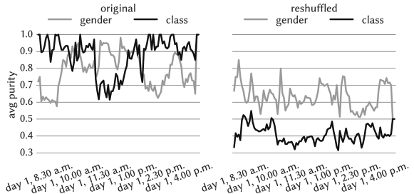
Figure 13. Temporal evolution (time on the $x$ axis) of average gender purity and average class purity ($y$ axis) of the maximal span-cores of the PrimarySchool dataset. Original data on the left, reshuffled data on the right.

Interaction length. Finally, we analyze the duration of interactions of social groups in schools by studying the distribution of the size of the span of the maximal span-cores of the three datasets (Figure 14). All distributions are extremely skewed with broad tails: most maximal span-cores have duration less than $1$ hour, but durations much larger than the average can also be observed. Interestingly, the three datasets at hand all exhibit the same functional shape, confirming a robust statistical behavior. We also note that similar robust broad distributions have been observed for simpler characteristics of human interactions such as the statistics of contact durations (Stehlé et al., 2011; Mastrandrea et al., 2015). Outliers appear also at very large durations, especially for the HongKong dataset that has maximal span-cores lasting up to $83$ hours. Group interactions of such long span are clearly abnormal and represent outliers in the distributions. We will show, in the following of this section, how to exploit such outliers to detect both irregular interactions and anomalous temporal intervals.

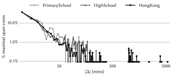
Figure 14. Distribution of the size of the span $|\Delta|$ of the maximal span-cores. The $x$ axis reports the size of the span (in minutes), while the $y$ axis the percentage of maximal span-cores having a given size of the span.

8.2. Anomaly detection

The identification of anomalous behaviors in temporal networks has been the focus of several studies in the last few years (Mongiovi et al., 2013; Sapienza et al., 2015). Based on the above findings, we devise a simple procedure to detect anomalous edges and intervals of the HongKong dataset that exploits maximal span-cores. The topmost plot of Figure 15 reports the number of edges for each timestamp of the original HongKong dataset. It is easy to notice that there is a lot of constant anomalous activity between school days and during the weekend, i.e., days six and seven: unexpectedly, the number of interactions per timestamp does not drop to zero. This happened in fact because proximity sensors were left in each class and close to each other, at the end of the lessons. In order to automatically detect these steady activity patterns that do not correspond to any genuine social dynamics, we apply the following procedure: $(i)$ find a set of anomalously long temporal intervals supporting maximal span-cores, $(ii)$ identify anomalous vertices, and, $(iii)$ filter out anomalous edges.

The first step of this procedure requires to find the set of temporal intervals $\mathcal{I}=\{\Delta\sqsubseteq T\mid C_{k,\Delta}\in\mathbf{C}_{M}\land|\Delta|>tr\}$ that are the span of a maximal span-core $C_{k,\Delta}$ with size longer than a certain threshold $tr$. Then, for each timestamp $t\in T$, select as anomalous all those vertices that appear in the span-cores $\{C_{1,\Delta}\mid\Delta\in\mathcal{I}\land t\in\Delta\}$, i.e., the span-cores of $k=1$ whose span is in $\mathcal{I}$ and contains $t$. Finally, at each timestamp $t\in T$, remove edges that are incident to at least a vertex that has been marked as anomalous at time $t$. Consistently with the distribution of the span durations of the maximal span-cores, we select the threshold $tr=22$ ($110$ minutes). The results of this filtering procedure are shown in the middle plot of Figure 15. The number of edges during school days remains approximately unchanged, while the activity noticeably decreases in-between. Identifying as positives the spurious interactions occurring when the school is closed and as negatives the genuine interactions observed when the school is open, this approach achieves a precision of $0.91$ and a recall of $0.64$.

We can refine this anomaly detection process by identifying, in addition to anomalous edges, also anomalous temporal intervals. We define a timestamp $t\in T$ as anomalous if the ratio between the number of original edges (top plot of Figure 15) and the number of filtered edges (middle plot of Figure 15) exceeds a given threshold. We apply this further filtering to the HongKong dataset with a threshold of $1.5$ and report the results in the bottommost plot of Figure 15. The number of edges when the school is closed drops to zero, while the activity during school days is not modified, except for the last one, which is affected by the proximity to the end of the time domain. The overall procedure yields a slightly higher value of precision, $0.93$, and substantially improves the recall to $0.99$.

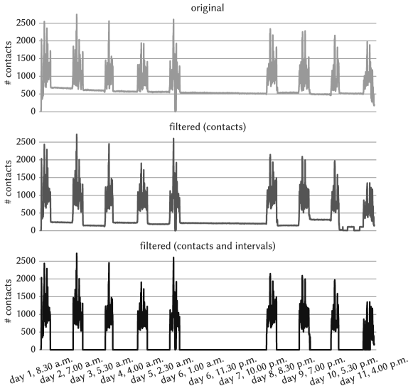
Figure 15. HongKong dataset: number of edges per timestamp in the original data (top), after filtering anomalous edges (middle), and after filtering anomalous edges and intervals (bottom). Days 6 and 7 are weekend.

8.3. Graph embedding and vertex classification

In this subsection we show how Temporal Community Search can be profitably exploited for classifying the vertices of a temporal graph. Specifically, the classification framework we set up is based on the paradigm of graph embedding, which has attracted a great deal of attention in the last few years, and whose goal is to assign to every vertex of a graph a numerical vector (i.e., an embedding) such that structurally similar vertices are represented by similar vectors, and vice versa (Grover and Leskovec, 2016; Epasto and Perozzi, 2019; Goyal and Ferrara, 2018). Here, our framework simply consists in learning suitable embeddings for the vertices of the input graph, and then give them as input to some (well-established) classifier to ultimately accomplish the desired classification task. Thus, the main goal is to learn embeddings that are well-representative of the relationships among vertices, so as to help the classifier perform accurately. As our main result here, we show how an embedding strategy based on a simple exploitation of the output of Temporal Community Search achieves results comparable to well-established vertex-embedding methods such as DeepWalk (Perozzi et al., 2014), LINE (Tang et al., 2015), and node2vec (Grover and Leskovec, 2016).

Method. For every vertex of the input temporal graph, we build an embedding as an $h$-dimensional vector conveying the information provided by a solution to the Temporal Community Search problem on the same graph. Specifically, consider a vertex $u\in V$ and a solution $\{\langle S_{i},\Delta_{i}\rangle\}_{i=1}^{h}$ to Temporal Community Search on query-vertex set $Q=\{u\}$. We define $u$’s embedding as

$$\mathbf{X}_{u}=[v^{*}_{Q,\Delta_{1}},v^{*}_{Q,\Delta_{2}},\ldots,v^{*}_{Q,\Delta_{h}}],$$

which corresponds to the temporally-ordered sequence of minimum degrees of the $h$ communities identified by the temporal-community-search solution. Below we show that this simple approach is sufficient to achieve interesting experimental results. Clearly, more sophisticated methods are possible, e.g., by simultaneously exploiting information from the $S_{i}$ communities. However, our main goal here is to give an idea of how the Temporal Community Search problem can be successfully leveraged in a relevant application scenario, rather than devise the best temporal-community-search-based graph-embedding method.

PrimarySchool

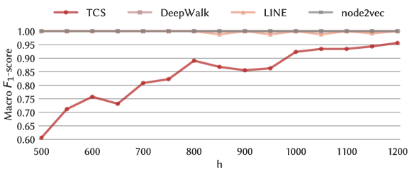
HighSchool

Figure 16. Vertex classification: Macro $F_{1}$-score of the proposed temporal-community-search-based graph-embedding method TCS and the competing methods, with varying the dimensionality $h$ of the output embeddings, on the PrimarySchool and HighSchool datasets.

Evaluation. We assess the performance of our method on the PrimarySchool and HighSchool datasets. In these datasets vertices correspond to students, and vertex labels (to be predicted) are the classes that every student belongs to. We involve in the comparison the following state-of-the-art vertex-embedding methods:

• DeepWalk (Perozzi et al., 2014), a method that preserves the proximity between vertices by running a set of random walks and maximizing the sum of the log-likelihood of a set of vertices for each walk.

• LINE (Tang et al., 2015), which optimizes a suitable objective function preserving both first-order (one-hop) and second-order (two-hop) proximities. Neighborhoods are not explored via random walk, but in a breadth-first fashion.

• node2vec (Grover and Leskovec, 2016), which is based on the same idea underlying DeepWalk, but allowing more flexibility on how random walks explore and leave the neighborhood of the current vertex.

These three methods consider non-temporal graphs. Therefore, we feed them with aggregated graphs in which every edge exists if it exists in at least one timestamp.

Exhaustive grid search is carried out to tune parameters of node2vec (Grover and Leskovec, 2016) and DeepWalk (Perozzi et al., 2014). In particular, for both methods, we tune the neighborhood parameters of a vertex, i.e., number of walks $r$, and walk length $l$, while the neighborhood size $k$ is set to $10$. Furthermore, for node2vec we tune the return and in-out parameters $p$ and $q$. For each parameter, we use the same grid of values as the one considered in the parameter sensitivity analysis reported in the original node2vec paper (Grover and Leskovec, 2016). Specifically, we consider the following parameter space:

• Number of walks, $r=\{6,8,10,12,14,16,18,20\}$;

• Walk length, $l=\{30,40,50,60,70,80,90,100,110\}$;

• Return parameter, $p=\{0.25,0.5,1,2,4\}$;

• In-out parameter, $q=\{0.25,0.5,1,2,4\}$.

We select the combination of parameters maximizing the Macro $F_{1}$-score averaged over a range of numbers of latent dimensions $d=\{16,32,64,128,256\}$.

After filtering out those vertices representing the teachers, we partition the remaining vertices (i.e., the students) into training and test sets with an 80-20 split. A standard scaler is applied to the features extracted by each embedding method and, then, a penalized logistic-regression classifier is trained.

In Figure 16 we report classification results in terms of Macro $F_{1}$-score, with varying the dimensionality $h$ of the embeddings. On the PrimarySchool dataset, for $h\geq 200$, our TCS has performance close to $1$ in terms Macro $F_{1}$-score, similarly to the three baselines. It can be observed that the TCS results are better as $h$ gets higher; in particular, TCS is even better than node2vec for $h=|T|$. This is expected and is motivated as, for higher $h$, TCS is allowed to rely on more temporal information about the vertices. On the HighSchool dataset, TCS is outperformed by all methods for smaller $h$. However, again, the performance of TCS becomes competitive for larger $h$, up to achieving comparable results to the best method(s) for $h=|T|$.

9. Conclusions

Temporal networks are a powerful representation of how relations are established and interrupted along time among a given population of entities. An interesting primitive for analyzing this type of networks is the extraction of relevant patterns, such as dense subgraphs, together with their time interval of existence (or span). Following this idea, we introduced in this paper a notion of temporal core decomposition where each core is associated with its span. Exploiting containment properties among cores we developed efficient algorithms for computing all the span-cores, and also only the maximal ones. We then introduced the problem of temporal community search and showed how it can be solved in polynomial time via dynamic programming. We also proved an interesting connection between temporal community search and maximal span-cores, which made it possible to devise a considerably more efficient algorithm than the naïve dynamic-programming one. Finally, we presented applications on empirical networks of human close-range proximity, that illustrate the relevance of the notions of (maximal) span-core and temporal community search in a variety analyses and applications.

In future work we will study the role of maximal span-cores with large coreness and/or $|\Delta|$ in spreading processes on temporal networks. Furthermore, span-cores represent features that can be used for network fingerprinting and classification, as well as for model validation, and that could provide support for new ways of visualizing large-scale time-varying graphs. We also plan to investigate different semantics of temporal patterns and the corresponding notions of core decompositions extracted from temporal networks, such as, for instance, the ones that might arise by considering a temporal edge existing in a given interval if it appears in at least one of the timestamps of the interval, or in a fraction of timestamps larger than a given threshold. Finally, investigation in temporal community search has just started: we plan to study different notions of community search and their corresponding extraction problems. As an example, a variant of the notion adopted in this article, which is worth to be investigated further, would correspond to relaxing the requirement of covering the whole temporal domain $T$, and instead looking for a set of communities giving a good enough temporal coverage.

References

- (1)
- Akoglu et al. (2013) Leman Akoglu, Duen Horng Chau, Christos Faloutsos, Nikolaj Tatti, Hanghang Tong, and Jilles Vreeken. 2013. Mining Connection Pathways for Marked Nodes in Large Graphs. In Proc. of SIAM Int. Conf. on Data Mining (SDM). 37–45.
- Alvarez-Hamelin et al. (2006) J Ignacio Alvarez-Hamelin, Luca Dall’Asta, Alain Barrat, and Alessandro Vespignani. 2006. Large scale networks fingerprinting and visualization using the k-core decomposition. In Proc. of Conf. on Advances in Neural Information Processing Systems (NeurIPS). 41–50.
- Andersen and Chellapilla (2009) Reid Andersen and Kumar Chellapilla. 2009. Finding Dense Subgraphs with Size Bounds. In Proc. of Int. Work. on Algorithms and Models for the Web-Graph (WAW). 25–37.
- Andersen and Lang (2006) Reid Andersen and Kevin J. Lang. 2006. Communities from seed sets. In Proc. of World Wide Web Conf. (WWW). 223–232.
- Angel et al. (2012) Albert Angel, Nikos Sarkas, Nick Koudas, and Divesh Srivastava. 2012. Dense subgraph maintenance under streaming edge weight updates for real-time story identification. Proc. of the VLDB Endowment (PVLDB) 5, 6 (2012), 574–585.
- Bader and Hogue (2003) Gary D. Bader and Christopher W. V. Hogue. 2003. An automated method for finding molecular complexes in large protein interaction networks. BMC Bioinformatics 4 (2003), 2.
- Barbieri et al. (2015) Nicola Barbieri, Francesco Bonchi, Edoardo Galimberti, and Francesco Gullo. 2015. Efficient and effective community search. Data Mining and Knowledge Discovery (DAMI) 29, 5 (2015), 1406–1433.
- Batagelj et al. (1999) Vladimir Batagelj, Andrej Mrvar, and Matjaz Zaversnik. 1999. Partitioning Approach to Visualization of Large Graphs. In Proc. of Int. Symp. on Graph Drawing (GD). 90–97.
- Batagelj and Zaversnik (2011) Vladimir Batagelj and Matjaz Zaversnik. 2011. Fast algorithms for determining (generalized) core groups in social networks. Advances in Data Analysis and Classification (ADAC) 5, 2 (2011), 129–145.
- Bellman (1961) R. Bellman. 1961. On the Approximation of Curves by Line Segments Using Dynamic Programming. Communications of the ACM (CACM) 4, 6 (1961), 284.
- Bentert et al. (2018) Matthias Bentert, Anne-Sophie Himmel, Hendrik Molter, Marco Marik, Rolf Niedermeier, and René Saitenmacher. 2018. Listing all maximal k-plexes in temporal graphs. In Proc. of. IEEE/ACM Int. Conf. on Advances in Social Networks Analysis and Mining (ASONAM). 41–46.
- Berlingerio et al. (2009) Michele Berlingerio, Francesco Bonchi, Björn Bringmann, and Aristides Gionis. 2009. Mining Graph Evolution Rules. In Proc. of Europ. Machine Learning and Principles and Practice of Knowledge Discovery in Databases (ECML PKDD). 115–130.
- Bian et al. (2018) Yuchen Bian, Yaowei Yan, Wei Cheng, Wei Wang, Dongsheng Luo, and Xiang Zhang. 2018. On Multi-query Local Community Detection. In Proc. of IEEE Int. Conf. on Data Mining (ICDM). 9–18.
- Bogdanov et al. (2011) Petko Bogdanov, Misael Mongiovì, and Ambuj K Singh. 2011. Mining heavy subgraphs in time-evolving networks. In Proc. of IEEE Int. Conf. on Data Mining (ICDM). 81–90.
- Bonchi et al. (2016) Francesco Bonchi, Ilaria Bordino, Francesco Gullo, and Giovanni Stilo. 2016. Identifying Buzzing Stories via Anomalous Temporal Subgraph Discovery. In Proc. of IEEE/WIC/ACM Int. Conf. on Web Intelligence (WI). 161–168.
- Bonchi et al. (2019) Francesco Bonchi, Ilaria Bordino, Francesco Gullo, and Giovanni Stilo. 2019. The importance of unexpectedness: Discovering buzzing stories in anomalous temporal graphs. Web Intelligence 17, 3 (2019), 177–198.
- Bonchi et al. (2015) Francesco Bonchi, Aristides Gionis, Francesco Gullo, Charalampos E. Tsourakakis, and Antti Ukkonen. 2015. Chromatic Correlation Clustering. ACM Transactions on Knowledge Discovery from Data (TKDD) 9, 4 (2015), 34:1–34:24.
- Bonchi et al. (2018) Francesco Bonchi, Francesco Gullo, and Andreas Kaltenbrunner. 2018. Core Decomposition of Massive, Information-Rich Graphs. In Encyclopedia of Social Network Analysis and Mining, 2nd Edition, Reda Alhajj and Jon G. Rokne (Eds.). Springer.
- Bonchi et al. (2014) Francesco Bonchi, Francesco Gullo, Andreas Kaltenbrunner, and Yana Volkovich. 2014. Core decomposition of uncertain graphs. In Proc. of ACM Int. Conf. on Knowledge Discovery and Data Mining (KDD). 1316–1325.
- Bringmann et al. (2010) Björn Bringmann, Michele Berlingerio, Francesco Bonchi, and Aristides Gionis. 2010. Learning and Predicting the Evolution of Social Networks. IEEE Intelligent Systems 25, 4 (2010), 26–35.
- Charikar (2000) Moses Charikar. 2000. Greedy approximation algorithms for finding dense components in a graph. In Proc. of Int. Work. on Approximation Algorithms for Combinatorial Optimization Problems (APPROX). 84–95.
- Charikar et al. (2018) Moses Charikar, Yonatan Naamad, and Jimmy Wu. 2018. On Finding Dense Common Subgraphs. CoRR abs/1802.06361 (2018).
- Cheng et al. (2011) James Cheng, Yiping Ke, Shumo Chu, and M. Tamer Özsu. 2011. Efficient core decomposition in massive networks. In Proc. of IEEE Int. Conf. on Data Engineering (ICDE). 51–62.
- Cui et al. (2014) Wanyun Cui, Yanghua Xiao, Haixun Wang, and Wei Wang. 2014. Local search of communities in large graphs. In Proc. of ACM Int. Conf. on Management of Data (SIGMOD). 991–1002.
- Das Sarma et al. (2011) Anish Das Sarma, Alpa Jain, and Cong Yu. 2011. Dynamic relationship and event discovery. In Proc. of Int. Conf. on Web Search and Data Mining (WSDM). 207–216.
- Desmier et al. (2012) Elise Desmier, Marc Plantevit, Céline Robardet, and Jean-François Boulicaut. 2012. Cohesive co-evolution patterns in dynamic attributed graphs. In Proc. of Int. Conf. on Discovery Science (DS). 110–124.
- Dickison et al. (2016) Mark E. Dickison, Matteo Magnani, and Luca Rossi. 2016. Multilayer social networks. Cambridge University Press.
- Eidsaa and Almaas (2013) Marius Eidsaa and Eivind Almaas. 2013. -core network decomposition: A generalization of -core analysis to weighted networks. Physical Review E 88 (2013), 062819. Issue 6.
- Epasto et al. (2015) Alessandro Epasto, Silvio Lattanzi, and Mauro Sozio. 2015. Efficient densest subgraph computation in evolving graphs. In Proc. of World Wide Web Conf. (WWW). 300–310.
- Epasto and Perozzi (2019) Alessandro Epasto and Bryan Perozzi. 2019. Is a Single Embedding Enough? Learning Node Representations that Capture Multiple Social Contexts. In Proc. of World Wide Web Conf. (WWW). 394–404.
- Eppstein et al. (2010) David Eppstein, Maarten Löffler, and Darren Strash. 2010. Listing All Maximal Cliques in Sparse Graphs in Near-Optimal Time. In Proc. of Int. Symp. on Algorithms and Computation (ISAAC). 403–414.
- Érdi et al. (2013) Péter Érdi, Kinga Makovi, Zoltán Somogyvári, Katherine Strandburg, Jan Tobochnik, Péter Volf, and László Zalányi. 2013. Prediction of emerging technologies based on analysis of the US patent citation network. Scientometrics 95, 1 (2013), 225–242.
- Faloutsos et al. (2004) Christos Faloutsos, Kevin S. McCurley, and Andrew Tomkins. 2004. Fast discovery of connection subgraphs. In Proc. of ACM Int. Conf. on Knowledge Discovery and Data Mining (KDD). 118–127.
- Fang et al. (2017a) Yixiang Fang, Reynold Cheng, Yankai Chen, Siqiang Luo, and Jiafeng Hu. 2017a. Effective and efficient attributed community search. The VLDB Journal 26, 6 (2017), 803–828.
- Fang et al. (2017b) Yixiang Fang, Reynold Cheng, Xiaodong Li, Siqiang Luo, and Jiafeng Hu. 2017b. Effective community search over large spatial graphs. Proc. of the VLDB Endowment (PVLDB) 10, 6 (2017), 709–720.
- Fang et al. (2020) Yixiang Fang, Xin Huang, Lu Qin, Ying Zhang, Wenjie Zhang, Reynold Cheng, and Xuemin Lin. 2020. A survey of community search over big graphs. The VLDB Journal 29, 1 (2020), 353–392.
- Galimberti et al. (2018) Edoardo Galimberti, Alain Barrat, Francesco Bonchi, Ciro Cattuto, and Francesco Gullo. 2018. Mining (maximal) span-cores from temporal networks. In Proc. of Int. Conf. on Information and Knowledge Management (CIKM). 107–116.
- Galimberti et al. (2017) Edoardo Galimberti, Francesco Bonchi, and Francesco Gullo. 2017. Core Decomposition and Densest Subgraph in Multilayer Networks. In Proc. of Int. Conf. on Information and Knowledge Management (CIKM). 1807–1816.
- Galimberti et al. (2020) Edoardo Galimberti, Francesco Bonchi, Francesco Gullo, and Tommaso Lanciano. 2020. Core Decomposition in Multilayer Networks: Theory, Algorithms, and Applications. ACM Transactions on Knowledge Discovery from Data (TKDD) 14, 1 (2020), 11:1–11:40.
- Garas et al. (2012) Antonios Garas, Frank Schweitzer, and Shlomo Havlin. 2012. A k-shell decomposition method for weighted networks. New Journal of Physics (NJP) 14, 8 (2012), 083030.
- García et al. (2013) David García, Pavlin Mavrodiev, and Frank Schweitzer. 2013. Social resilience in online communities: the autopsy of Friendster. In Proc. of ACM Conf. on Online Social Networks (COSN). 39–50.
- Gauvin et al. (2014) Laetitia Gauvin, André Panisson, and Ciro Cattuto. 2014. Detecting the community structure and activity patterns of temporal networks: a non-negative tensor factorization approach. PLOS ONE 9, 1 (2014), e86028.
- Gemmetto et al. (2014) Valerio Gemmetto, Alain Barrat, and Ciro Cattuto. 2014. Mitigation of infectious disease at school: targeted class closure vs school closure. BMC Infectious Diseases 14, 1 (2014), 695.
- Giatsidis et al. (2013) Christos Giatsidis, Dimitrios M. Thilikos, and Michalis Vazirgiannis. 2013. D-cores: measuring collaboration of directed graphs based on degeneracy. Knowledge and Information Systems (KAIS) 35, 2 (2013), 311–343.
- Goyal and Ferrara (2018) Palash Goyal and Emilio Ferrara. 2018. Graph embedding techniques, applications, and performance: A survey. Knowledge-Based Systems 151 (2018), 78–94.
- Grover and Leskovec (2016) Aditya Grover and Jure Leskovec. 2016. node2vec: Scalable feature learning for networks. In Proc. of ACM Int. Conf. on Knowledge Discovery and Data Mining (KDD). 855–864.
- Healy et al. (2006) John Healy, Jeannette Janssen, Evangelos E. Milios, and William Aiello. 2006. Characterization of Graphs Using Degree Cores. In Proc. of Int. Work. on Algorithms and Models for the Web-Graph (WAW). 25–37.
- Himmel et al. (2016) Anne-Sophie Himmel, Hendrik Molter, Rolf Niedermeier, and Manuel Sorge. 2016. Enumerating maximal cliques in temporal graphs. In Proc. of. IEEE/ACM Int. Conf. on Advances in Social Networks Analysis and Mining (ASONAM). 337–344.
- Huang et al. (2014) Xin Huang, Hong Cheng, Lu Qin, Wentao Tian, and Jeffrey Xu Yu. 2014. Querying k-truss community in large and dynamic graphs. In Proc. of ACM Int. Conf. on Management of Data (SIGMOD). 1311–1322.
- Huang and Lakshmanan (2017) Xin Huang and Laks VS Lakshmanan. 2017. Attribute-driven community search. Proc. of the VLDB Endowment (PVLDB) 10, 9 (2017), 949–960.
- Huang et al. (2017) Xin Huang, Laks VS Lakshmanan, and Jianliang Xu. 2017. Community search over big graphs: Models, algorithms, and opportunities. In Proc. of IEEE Int. Conf. on Data Engineering (ICDE). 1451–1454.
- Inokuchi and Washio (2010) Akihiro Inokuchi and Takashi Washio. 2010. Mining frequent graph sequence patterns induced by vertices. In Proc. of SIAM Int. Conf. on Data Mining (SDM). 466–477.
- Jethava and Beerenwinkel (2015) Vinay Jethava and Niko Beerenwinkel. 2015. Finding dense subgraphs in relational graphs. In Proc. of Europ. Machine Learning and Principles and Practice of Knowledge Discovery in Databases (ECML PKDD). 641–654.
- Kitsak et al. (2010) Maksim Kitsak, Lazaros K. Gallos, Shlomo Havlin, Fredrik Liljeros, Lev Muchnik, H. Eugene Stanley, and Hernán A. Makse. 2010. Identifying influential spreaders in complex networks. Nature Physics 6, 11 (2010), 888–893.
- Kloumann and Kleinberg (2014) Isabel M. Kloumann and Jon M. Kleinberg. 2014. Community membership identification from small seed sets. In Proc. of ACM Int. Conf. on Knowledge Discovery and Data Mining (KDD). 1366–1375.
- Kortsarz and Peleg (1994) Guy Kortsarz and David Peleg. 1994. Generating Sparse 2-Spanners. Journal of Algorithms 17, 2 (1994), 222–236.
- Kovanen et al. (2011) Lauri Kovanen, Márton Karsai, Kimmo Kaski, János Kertész, and Jari Saramäki. 2011. Temporal motifs in time-dependent networks. Journal of Statistical Mechanics 2011, 11 (2011), P11005.
- Leung et al. (2010) Cane Wing-ki Leung, Ee-Peng Lim, David Lo, and Jianshu Weng. 2010. Mining interesting link formation rules in social networks. In Proc. of Int. Conf. on Information and Knowledge Management (CIKM). 209–218.
- Li et al. (2018) Rong-Hua Li, Jiao Su, Lu Qin, Jeffrey Xu Yu, and Qiangqiang Dai. 2018. Persistent community search in temporal networks. In Proc. of IEEE Int. Conf. on Data Engineering (ICDE). 797–808.
- Li et al. (2014) Rong-Hua Li, Jeffrey Xu Yu, and Rui Mao. 2014. Efficient core maintenance in large dynamic graphs. IEEE Transactions on Knowledge and Data Engineering (TKDE) 26, 10 (2014), 2453–2465.
- Liu et al. (2019b) Boge Liu, Long Yuan, Xuemin Lin, Lu Qin, Wenjie Zhang, and Jingren Zhou. 2019b. Efficient (, )-core Computation: an Index-based Approach. In Proc. of World Wide Web Conf. (WWW). 1130–1141.
- Liu et al. (2019a) Paul Liu, Austin R Benson, and Moses Charikar. 2019a. Sampling Methods for Counting Temporal Motifs. In Proc. of Int. Conf. on Web Search and Data Mining (WSDM). 294–302.
- Ma et al. (2017) Shuai Ma, Renjun Hu, Luoshu Wang, Xuelian Lin, and Jinpeng Huai. 2017. Fast Computation of Dense Temporal Subgraphs. In Proc. of IEEE Int. Conf. on Data Engineering (ICDE). 361–372.
- Malliaros et al. (2020) Fragkiskos D. Malliaros, Christos Giatsidis, Apostolos N. Papadopoulos, and Michalis Vazirgiannis. 2020. The Core Decomposition of Networks: Theory, Algorithms and Applications. The VLDB Journal 29, 1 (2020), 61–92.
- Maslov and Sneppen (2002) Sergei Maslov and Kim Sneppen. 2002. Specificity and stability in topology of protein networks. Science 296, 5569 (2002), 910–913.
- Mastrandrea et al. (2015) Rossana Mastrandrea, Julie Fournet, and Alain Barrat. 2015. Contact Patterns in a High School: A Comparison between Data Collected Using Wearable Sensors, Contact Diaries and Friendship Surveys. PLOS ONE 10, 9 (09 2015), 1–26.
- Matula and Beck (1983) David W. Matula and Leland L. Beck. 1983. Smallest-Last Ordering and clustering and Graph Coloring Algorithms. Journal of the ACM (JACM) 30, 3 (1983), 417–427.
- Mongiovi et al. (2013) Misael Mongiovi, Petko Bogdanov, Razvan Ranca, Evangelos E Papalexakis, Christos Faloutsos, and Ambuj K Singh. 2013. Netspot: Spotting significant anomalous regions on dynamic networks. In Proc. of SIAM Int. Conf. on Data Mining (SDM). 28–36.
- Montresor et al. (2013) Alberto Montresor, Francesco De Pellegrini, and Daniele Miorandi. 2013. Distributed k-Core Decomposition. IEEE Transactions on Parallel and Distributed Systems (TPDS) 24, 2 (2013), 288–300.
- Perozzi et al. (2014) Bryan Perozzi, Rami Al-Rfou, and Steven Skiena. 2014. Deepwalk: Online learning of social representations. In Proc. of ACM Int. Conf. on Knowledge Discovery and Data Mining (KDD). 701–710.
- Reinthal et al. (2016) Alexander Reinthal, Arvid Andersson, Erik Norlander, Philip Stålhammar, Sebastian Norlin, et al. 2016. Finding the Densest Common Subgraph with Linear Programming. (2016).
- Rozenshtein et al. (2018) Polina Rozenshtein, Francesco Bonchi, Aristides Gionis, Mauro Sozio, and Nikolaj Tatti. 2018. Finding events in temporal networks: Segmentation meets densest-subgraph discovery. In Proc. of IEEE Int. Conf. on Data Mining (ICDM). 397–406.
- Rozenshtein et al. (2017) Polina Rozenshtein, Nikolaj Tatti, and Aristides Gionis. 2017. Finding dynamic dense subgraphs. ACM Transactions on Knowledge Discovery from Data (TKDD) 11, 3 (2017), 27.
- Ruchansky et al. (2015) Natali Ruchansky, Francesco Bonchi, David García-Soriano, Francesco Gullo, and Nicolas Kourtellis. 2015. The minimum wiener connector problem. In Proc. of ACM Int. Conf. on Management of Data (SIGMOD). 1587–1602.
- Ruchansky et al. (2017) Natali Ruchansky, Francesco Bonchi, David García-Soriano, Francesco Gullo, and Nicolas Kourtellis. 2017. To Be Connected, or Not to Be Connected: That is the Minimum Inefficiency Subgraph Problem. In Proc. of Int. Conf. on Information and Knowledge Management (CIKM). 879–888.
- Sapienza et al. (2015) Anna Sapienza, André Panisson, Joseph Wu, Laetitia Gauvin, and Ciro Cattuto. 2015. Detecting anomalies in time-varying networks using tensor decomposition. In Proc. of IEEE Int. Conf. on Data Mining - Worskshops (ICDMW). 516–523.
- Sariyüce et al. (2013) Ahmet Erdem Sariyüce, Bugra Gedik, Gabriela Jacques-Silva, Kun-Lung Wu, and Ümit V. Çatalyürek. 2013. Streaming Algorithms for k-core Decomposition. Proc. of the VLDB Endowment (PVLDB) 6, 6 (2013), 433–444.
- Semertzidis et al. (2018) Konstantinos Semertzidis, Evaggelia Pitoura, Evimaria Terzi, and Panayiotis Tsaparas. 2018. Finding lasting dense subgraphs. Data Mining and Knowledge Discovery (DAMI) 33, 5 (2018), 1417–1445.
- Sozio and Gionis (2010) Mauro Sozio and Aristides Gionis. 2010. The community-search problem and how to plan a successful cocktail party. In Proc. of ACM Int. Conf. on Knowledge Discovery and Data Mining (KDD). 939–948.
- Stehlé et al. (2013) Juliette Stehlé, François Charbonnier, Tristan Picard, Ciro Cattuto, and Alain Barrat. 2013. Gender homophily from spatial behavior in a primary school: A sociometric study. Social Networks 35, 4 (2013), 604–613.
- Stehlé et al. (2011) Juliette Stehlé, Nicolas Voirin, Alain Barrat, Ciro Cattuto, Lorenzo Isella, Jean-François Pinton, Marco Quaggiotto, Wouter Van den Broeck, Corinne Régis, Bruno Lina, and Philippe Vanhems. 2011. High-Resolution Measurements of Face-to-Face Contact Patterns in a Primary School. PLOS ONE 6, 8 (2011), e23176.
- Tagarelli et al. (2017) Andrea Tagarelli, Alessia Amelio, and Francesco Gullo. 2017. Ensemble-based community detection in multilayer networks. Data Mining and Knowledge Discovery (DAMI) 31, 5 (2017), 1506–1543.
- Tang et al. (2015) Jian Tang, Meng Qu, Mingzhe Wang, Ming Zhang, Jun Yan, and Qiaozhu Mei. 2015. Line: Large-scale information network embedding. In Proc. of World Wide Web Conf. (WWW). 1067–1077.
- Tong and Faloutsos (2006) Hanghang Tong and Christos Faloutsos. 2006. Center-piece subgraphs: problem definition and fast solutions. In Proc. of ACM Int. Conf. on Knowledge Discovery and Data Mining (KDD). 404–413.
- Viard et al. (2016) Tiphaine Viard, Matthieu Latapy, and Clémence Magnien. 2016. Computing maximal cliques in link streams. Theoretical Computer Science (TCS) 609 (2016), 245–252.
- Wu et al. (2015) Huanhuan Wu, James Cheng, Yi Lu, Yiping Ke, Yuzhen Huang, Da Yan, and Hejun Wu. 2015. Core decomposition in large temporal graphs. In Proc. of IEEE Int. Conf. on Big Data. 649–658.
- Wuchty and Almaas (2005) Stefan Wuchty and Eivind Almaas. 2005. Peeling the yeast protein network. Proteomics 5, 2 (2005), 444–449.
- Yan et al. (2019) Yaowei Yan, Yuchen Bian, Dongsheng Luo, Dongwon Lee, and Xiang Zhang. 2019. Constrained Local Graph Clustering by Colored Random Walk. In Proc. of World Wide Web Conf. (WWW). 2137–2146.
- Zhang et al. (2017) Fan Zhang, Ying Zhang, Lu Qin, Wenjie Zhang, and Xuemin Lin. 2017. When engagement meets similarity: efficient (k, r)-core computation on social networks. Proc. of the VLDB Endowment (PVLDB) 10, 10 (2017), 998–1009.
- Zhang et al. (2010) Haohua Zhang, Hai Zhao, Wei Cai, Jie Liu, and Wanlei Zhou. 2010. Using the k-core decomposition to analyze the static structure of large-scale software systems. The Journal of Supercomputing 53, 2 (2010), 352–369.
- Zschoche et al. (2020) Philipp Zschoche, Till Fluschnik, Hendrik Molter, and Rolf Niedermeier. 2020. The complexity of finding small separators in temporal graphs. Journal of Computer and System Sciences (JCSS) 107 (2020), 72–92.