Variance reduction for Markov chains with application to MCMC

Abstract

In this paper we propose a novel variance reduction approach for additive functionals of Markov chains based on minimization of an estimate for the asymptotic variance of these functionals over suitable classes of control variates. A distinctive feature of the proposed approach is its ability to significantly reduce the overall finite sample variance. This feature is theoretically demonstrated by means of a deep non asymptotic analysis of a variance reduced functional as well as by a thorough simulation study. In particular we apply our method to various MCMC Bayesian estimation problems where it favourably compares to the existing variance reduction approaches.

1 Introduction

Variance reduction methods play nowadays a prominent role as a complexity reduction tool in simulation based numerical algorithms like Monte Carlo (MC) or Markov Chain Monte Carlo (MCMC). Introduction to many of variance reduction techniques can be found in Robert and Casella [32], Rubinstein and Kroese [36], Gobet [18], and Glasserman [17]. While variance reduction techniques for MC algorithms are well studied, MCMC algorithms are still waiting for efficient variance reduction methods. Recently one witnessed a revival of interest in this area with numerous applications to Bayesian statistics, see for example Dellaportas and Kontoyiannis [9], Mira et al. [26], Brosse et al. [7], and references therein. The main difficulty in constructing efficient variance reduction methods for MCMC lies in the dependence between the successive values of the underlying Markov chain which can significantly increase the overall variance and needs to be accounted for.

Suppose that we wish to compute $\pi(f)\overset{\text{\tiny def}}{=}\mathsf{E}_{\pi}\big{[}f(X)\big{]}$, where $X$ is a random vector with a distribution $\pi$ on $\mathsf{X}\subseteq\mathbb{R}^{d}$ and $f:\mathsf{X}\to\mathbb{R}$ with $f\in\mathrm{L}^{2}(\pi)$. Let $(X_{k})_{k\geq 0}$ be a time homogeneous Markov chain with values in $\mathsf{X}$. Denote by $P$ its Markov kernel and define for any bounded measurable function $f$

$$Pf(x)=\int_{\mathsf{X}}P(x,\mathrm{d}y)f(y)\,,\quad x\in\mathsf{X}.$$

Assume that $P$ has the unique invariant distribution $\pi$, that is, $\int_{\mathsf{X}}\pi(\mathrm{d}x)P(x,\mathrm{d}y)=\pi(\mathrm{d}y)$. Under appropriate conditions, the Markov kernel $P$ may be shown to converge to the stationary distribution $\pi$, that is, for any $x\in\mathsf{X}$,

$$\lim_{n\to\infty}\|P^{n}(x,\cdot)-\pi\|_{\operatorname{TV}}=0,$$

where $\|\mu-\nu\|_{\operatorname{TV}}=\sup_{A\in\mathcal{X}}|\mu(A)-\nu(A)|$ and $\mathcal{X}$ is the Borel $\sigma$-field associated to $\mathsf{X}$. More importantly, under rather weak assumptions, the ergodic averages

$$\pi_{n}(f)\overset{\text{\tiny def}}{=}n^{-1}\sum_{k=0}^{n-1}f(X_{k})$$

satisfy, for any initial distribution, a central limit theorem (CLT) of the form

$$\sqrt{n}\bigl{[}\pi_{n}(f)-\pi(f)\bigr{]}=n^{-1/2}\sum_{k=0}^{n-1}\bigl{[}f(X_{k})-\pi(f)\bigr{]}\xrightarrow{\mathcal{D}}\mathcal{N}\bigl{(}0,{V}_{\infty}(f)\bigr{)}$$

with the asymptotic variance ${V}_{\infty}(f)$ given by

$${V}_{\infty}(f)\overset{\text{\tiny def}}{=}\lim_{n\to\infty}n\,\mathsf{E}_{\pi}\bigl{[}\{\pi_{n}(f)-\pi(f)\}^{2}\bigr{]}=\mathsf{E}_{\pi}\bigl{[}\tilde{f}^{2}\bigr{]}+2\sum_{k=1}^{\infty}\mathsf{E}_{\pi}\bigl{[}\tilde{f}P^{k}\tilde{f}\bigr{]},$$ (1)

where $\tilde{f}=f-\pi(f)$. This motivates to use ergodic averages $\pi_{n}(f)$ as a natural estimate for $\pi(f)$. For a broader discussion of the Markov chain CLT and conditions under which CLT holds, see Jones [23], Roberts and Rosenthal [33], and Douc et al. [12].

One important and widely used class of variance reduction methods for Markov chains is the method of control variates which is based on subtraction of a zero-mean random variable (control variate) from $\pi_{n}(f)$. There are several methods to construct such control variates. If $\nabla\log\pi$ is known, one can use popular zero-variance control variates based on the Stein’s identity, see Assaraf and Caffarel [2] and Mira et al. [26]. A non-parametric extension of such control variates is suggested in Oates et al. [29] and Oates et al. [28]. Control variates can be also obtained using the Poisson equation. Namely, it was observed by Henderson [21] that the function $U_{g}\overset{\text{\tiny def}}{=}g-Pg$ has zero mean with respect to $\pi$, provided that $\pi(|g|)<\infty$. Then the choice $g=\hat{f}$ with $\hat{f}$ satisfying the so-called Poisson equation $\hat{f}(x)-P\hat{f}(x)=\tilde{f}(x)$ leads to $f-U_{\hat{f}}=f-\hat{f}+P\hat{f}=\pi(f)$ hence yielding a zero-variance control variate for the empirical mean under $\pi.$ Although the Poisson equation involves the quantity of interest $\pi(f)$ and can not be solved explicitly in most cases, the above idea still can be used to construct some approximations for the zero-variance control variate $\hat{f}(x)-P\hat{f}(x)$. For example, Henderson [21] proposed to compute approximations to the solution of the Poisson equation for specific Markov chains with particular emphasis on models arising in stochastic network theory. In Dellaportas and Kontoyiannis [9] and Brosse et al. [7] regression-type control variates are developed and studied for reversible Markov chains. It is assumed in Dellaportas and Kontoyiannis [9] that the one-step conditional expectations can be computed analytically for a set of basis functions. The authors in Brosse et al. [7] proposed another approach tailored to diffusion setting which does require the computation of integrals of basis functions and only involves the application of the underlying differential generator.

There is a fundamental issue related to the control variates method. Since one usually needs to consider a large class of control variates, one has to choose a criterion to select the “best” control variate from this class. In the literature, such a choice is often based on the least squares criterion or on the sample variance, see, for example, Mira et al. [26], Oates et al. [29], South et al. [37]. Note that such criteria can not properly take into account the correlation structure of the underlying Markov chain and hence can only reduce the first term in (1).

In this paper, we propose a novel variance reduction method for Markov chains based on the empirical spectral variance minimization. The proposed method can be viewed as a generalization of the approach in Belomestny et al. [5, 4] to Markov chains. In a nutshell, given a class of control variates $\mathcal{G}$, that is, functions $g\in\mathcal{G}$ with $\pi(g)=0$ we consider the estimator

$$\pi_{n}(f-\widehat{g}_{n})\overset{\text{\tiny def}}{=}n^{-1}\sum_{k=0}^{n-1}\{f(X_{k})-\widehat{g}_{n}(X_{k})\}$$

with $\widehat{g}_{n}\overset{\text{\tiny def}}{=}\operatornamewithlimits{argmin}_{g\in\mathcal{G}}V_{n}(f-g)$, where $V_{n}(f)$ stands for an estimator of the asymptotic variance $V_{\infty}(f)$ defined in (1). This generalization turns out to be challenging for at least two reasons. First, there is no simple way to estimate the asymptotic variance $V_{\infty}(f)$ for Markov chains. Due to inherent serial correlation, estimating $V_{\infty}(f)$ requires specific techniques such as spectral and batch means methods; see Flegal and Jones [15] for a survey on variance estimators and their statistical properties. Second, a nonasymptotic analysis of the estimate $\widehat{g}_{n}$ is highly nontrivial and requires careful treatment. We perform this analysis for a rather general class of geometrically ergodic Markov chains including the well known Unadjusted Langevin Algorithm (ULA), Metropolis-Adjusted Langevin Algorithm (MALA) and Random Walk Metropolis (RWM). In particular, we show that under some restrictions on $\mathcal{G}$, the rate of the excess for the asymptotic variance can be controlled with high probability as follows:

$$V_{\infty}(f-\widehat{g}_{n})-\inf_{g\in\mathcal{G}}V_{\infty}(f-g)=O\left(n^{-\alpha}\right)$$

for some $\alpha\in[1/2,1).$ Let us stress that our results are rather generic and can cover various types of control variates. Apart from a comprehensive theoretical analysis we conduct an extensive simulation study including Bayesian inference via MCMC for logistic regression, Gaussian mixtures and Bayesian inference of ODE models. We show that for various MCMC algorithms our approach leads to a further significant variance reduction as compared to the least-squares-type criteria.

The paper is organised as follows. In Section 2 we introduce a general empirical variance minimisation procedure for Markov chains and analyse its properties. In Section 3 we apply our theoretical results to a widely used ULA and MALA. In Section 4 we conduct a thorough numerical study of the proposed approach. Finally all proofs are collected in Section 5 and Appendix A.

Notations

Let $\|\cdot\|$ denote the standard Euclidean norm. We say that $f:\mathbb{R}^{d}\rightarrow\mathbb{R}$ is $L-$Lipschitz function if $|f(x)-f(x^{\prime})|\leq L\|x-x^{\prime}\|$ for any $x,x^{\prime}\in\mathbb{R}^{d}$.

For any probability measure $\xi$ on $(\mathsf{X},\mathcal{X})$, we denote by $\operatorname{P}_{\xi}$ the unique probability under which $(X_{n})_{n\geqslant 0}$ is a Markov chain with Markov kernel $P$ and initial distribution $\xi$. We denote by $\mathsf{E}_{\xi}$ the expectation under the distribution $\operatorname{P}_{\xi}$. For $\xi$ a probability measure on $(\mathsf{X},\mathcal{X})$ and $A\in\mathcal{X}$, we denote by $\xi P(A)=\int\xi(\mathrm{d}x)P(x,A)$; for $h:\mathsf{X}\to\mathbb{R}_{+}$ a measurable function, we denote by $Ph(x)=\int P(x,\mathrm{d}y)h(y)$. Given two Markov kernels $P$ and $Q$ on $\mathsf{X}\times\mathcal{X}$, where $\mathcal{X}$ is the Borel $\sigma$-field on $\mathsf{X}$, we define $PQ(x,A)=\iint P(x,\mathrm{d}y)Q(y,A)$. We also define $P^{n}$ inductively by $P^{n}=PP^{n-1}$. Let $W:\mathsf{X}\to\left[1,\infty\right)$ be a measurable function. The $W$-norm of a function $h:\mathsf{X}\to\mathbb{R}$ is defined as $\|h\|_{W}=\sup_{x\in\mathsf{X}}\{|h(x)|/W(x)\}$. For any two probability measures $\mu$ and $\nu$ on $(\mathsf{X},\mathcal{X})$ satisfying $\mu(W)<\infty$ and $\nu(W)<\infty$, the $W$-norm of $\mu-\nu$ is defined as $\left\|\mu-\nu\right\|_{W}=\sup_{\|f\|_{W}\leq 1}|\mu(f)-\nu(f)|$.

We also use the 2-Wasserstein distance and the Kullback-Leibler divergence in our analysis. The $2$-Wasserstein distance between probability measures $\mu$ and $\nu$ is denoted by $W_{2}(\mu,\nu)\overset{\text{\tiny def}}{=}\inf_{\zeta}\bigl{(}\int_{\mathsf{X}\times\mathsf{X}}\|x-y\|^{2}\,\mathrm{d}\zeta(x,y)\bigr{)}^{1/2}$, where the infimum is taken over all probability measures $\zeta$ on the product space $\mathsf{X}\times\mathsf{X}$ with marginal distributions $\mu$ and $\nu$. The Kullback-Leibler divergence for $\mu$ and $\nu$ is defined as $\operatorname{KL}(\mu\|\nu)=\mathsf{E}_{\mu}\big{[}\log(\mathrm{d}\mu/\mathrm{d}\nu)\big{]}$ if $\nu\ll\mu$ and $\operatorname{KL}(\mu\|\nu)=\infty$ otherwise. We say that the probability measure $\mu$ satisfies the transportation cost-information inequality $\operatorname{T}_{2}(\alpha)$ if there is a constant $\alpha>0$ such that for any probability measure $\nu$

$$W_{2}(\mu,\nu)\leq\sqrt{2\alpha\operatorname{KL}(\mu\|\nu)}.$$ (2)

For a real-valued function $h$ on $\mathsf{X}\subset\mathbb{R}^{d}$ and a $\sigma$-finite measure $\lambda$ on $(\mathsf{X},\mathcal{X})$ we write $\|h\|_{\mathrm{L}^{p}(\lambda)}=(\int_{\mathsf{X}}|h(x)|^{p}\lambda(\mathrm{d}x))^{1/p}$ with $1\leq p<\infty$. The set of all functions $h$ with $\|h\|_{\mathrm{L}^{p}(\lambda)}<\infty$ is denoted by $\mathrm{L}^{p}(\lambda)=\mathrm{L}^{p}(\mathsf{X},\lambda)$.

Finally, the Sobolev space is defined as $W^{s,p}(\mathsf{X})=\left\{u\in\mathrm{L}^{p}(\lambda):\operatorname{D}^{\alpha}u\in\mathrm{L}^{p}(\lambda),\ \forall|\alpha|\leqslant s\right\}$, where $\lambda$ is the Lebesgue measure, $\alpha=(\alpha_{1},\ldots,\alpha_{d})$ is a multi-index with $|\alpha|=\alpha_{1}+\ldots+\alpha_{d}$, and $\operatorname{D}^{\alpha}$ stands for differential operator of the form $\operatorname{D}^{\alpha}={\partial^{|\alpha|}}/{\partial x_{1}^{\alpha_{1}}\ldots\partial x_{d}^{\alpha_{d}}}$. Here all derivatives are understood in the weak sense. The weighted Sobolev space $W^{s,p}(\mathsf{X},\langle x\rangle^{\beta})$ for a polynomial weighting function $\langle x\rangle^{\beta}=(1+\|x\|^{2})^{\beta/2}$, $\beta\in\mathbb{R}$, is defined by

$$W^{s,p}(\mathsf{X},\langle x\rangle^{\beta})=\bigl{\{}u:\ u\cdot\langle x\rangle^{\beta}\in W^{s,p}(\mathsf{X})\bigr{\}}.$$ (3)

The Sobolev norm is defined as $\|u\|_{W^{s,p}(\mathsf{X},\langle x\rangle^{\beta})}=\sum_{|\alpha|\leq s}\bigl{\|}\operatorname{D}^{\alpha}\bigl{(}u\langle x\rangle^{\beta}\bigr{)}\bigr{\|}_{\mathrm{L}^{p}(\lambda)}$. We say that $U\subset W^{s,p}(\mathsf{X},\langle x\rangle^{\beta})$ is norm-bounded if there exists $c>0$, such that $\|u\|_{W^{s,p}(\mathsf{X},\langle x\rangle^{\beta})}\leq c$ for any $u\in U$.

In what follows, we use the symbol $\lesssim$ for inequality up to an absolute constant.

2 Main results

2.1 Empirical spectral variance minimisation (ESVM)

In this paper, we propose a novel approach to choose a control variate from the set $\mathcal{G}$ referred to as the Empirical Spectral Variance Minimisation (ESVM). To shorten notation, let us denote by $\mathcal{H}=\mathcal{H}(\mathcal{G})$ a class of functions $h(x)=f(x)-g(x)$, with $g\in\mathcal{G}$. The main idea of the ESVM approach is to select a control variate which minimizes a finite sample estimate for the asymptotic variance ${V}_{\infty}(h)$. There are several estimates for $V_{\infty}(h)$ available in the literature, see Flegal and Jones [15]. For the sake of clarity we consider only the spectral variance estimator which provides the most generic way to estimate $V_{\infty}(h)$. It is defined as follows. Let $P$ be a Markov kernel admitting a unique invariant probability $\pi$ and set $\tilde{h}\overset{\text{\tiny def}}{=}h-\pi(h)$ (assuming $\pi(|h|)<\infty$). For $s\in\mathbb{Z}_{+}$, define the stationary lag $s$ autocovariance $\rho_{\pi}^{(h)}(s)\overset{\text{\tiny def}}{=}\mathsf{E}_{\pi}\big{[}\tilde{h}(X_{s})\tilde{h}(X_{0})\big{]}$ and the lag $s$ sample autocovariance via

$$\hat{\rho}_{n}^{(h)}(s)\overset{\text{\tiny def}}{=}n^{-1}\sum_{k=0}^{n-s-1}\{h(X_{k})-\pi_{n}(h)\}\{h(X_{k+s})-\pi_{n}(h)\},$$ (4)

where $\pi_{n}(h)\overset{\text{\tiny def}}{=}n^{-1}\sum_{j=0}^{n-1}h(X_{j})$. The spectral variance estimator is based on truncation and weighting of the sample autocovariance function,

$${V}_{n}(h)\overset{\text{\tiny def}}{=}\sum_{s=-(b_{n}-1)}^{b_{n}-1}w_{n}(s)\hat{\rho}_{n}^{(h)}(|s|)\,,$$ (5)

where $w_{n}$ is the lag window and $b_{n}$ is the truncation point. The truncation point is a sequence of integers and the lag window is a kernel of the form $w_{n}(s)=w(s/b_{n})$, where $w$ is a symmetric non-negative function supported on $[-1,1]$ which fulfils $|w(s)|\leq 1$ for $s\in[-1,1]$ and $w(s)=1$ for $s\in[-1/2,1/2]$. Other possible choices of the lag window $w_{n}$ can be considered, see Flegal and Jones [15]. In the ESVM approach we choose a control variate by minimizing the spectral variance

$$\widehat{h}\overset{\text{\tiny def}}{=}\operatornamewithlimits{argmin}_{h\in\mathcal{H}}{V}_{n}(h).$$ (6)

As the class $\mathcal{H}$ can be too large making the resulting optimization problem (6) computationally intractable, we consider a smaller class. Given $\varepsilon>0$, let $\mathcal{H}_{\varepsilon}\subset\mathcal{H}$ consist of centres of the minimal $\varepsilon$-covering net of $\mathcal{H}$ with respect to the $\mathrm{L}^{2}(\pi)$ distance. Further set

$$\widehat{h}_{\varepsilon}\overset{\text{\tiny def}}{=}\operatornamewithlimits{argmin}_{h\in\mathcal{H}_{\varepsilon}}{V}_{n}(h).$$ (7)

In what follows, we assume that $\mathcal{H}$ is a norm-bounded set in $\mathrm{L}^{2}(\pi)$. Hence the set $\mathcal{H}_{\varepsilon}$ is finite. The estimates of the form (7) are referred to as skeleton or sieve estimates in the statistical literature (see, for example, Wong and Shen [39], Devroye et al. [10], and van de Geer [38]).

2.2 Theoretical analysis

In this section, we analyze the proposed ESVM procedure in terms of the excess of the asymptotic variance. Namely, we provide non-asymptotic bounds of the form:

$$V_{\infty}(\widehat{h}_{\varepsilon})-\inf_{h\in\mathcal{H}}V_{\infty}(h)=O\left(n^{-\alpha}\right),\quad 1/2<\alpha<1,$$ (8)

holding with high probability.

Before we proceed to theoretical results, let us define a quantity which is used to choose a radius $\varepsilon$ of the covering net $\mathcal{H}_{\varepsilon}$ over which $\widehat{h}_{\varepsilon}$ is computed. Given any $\varepsilon>0$, let $H_{\mathrm{L}^{2}(\pi)}(\mathcal{H},\varepsilon)$ be a metric entropy of $\mathcal{H}$ in $\mathrm{L}^{2}(\pi)$, that is, $H_{\mathrm{L}^{2}(\pi)}(\mathcal{H},\varepsilon)\overset{\text{\tiny def}}{=}\log|\mathcal{H}_{\varepsilon}|$, where $|\mathcal{H}_{\varepsilon}|$ is cardinality of $\mathcal{H}_{\varepsilon}$ (which is assumed to be finite). Define by $\gamma_{\mathrm{L}^{2}(\pi)}(\mathcal{H},n)$ a so-called fixed point

$$\gamma_{\mathrm{L}^{2}(\pi)}(\mathcal{H},n)\overset{\text{\tiny def}}{=}\inf\{\eta>0:\ H_{\mathrm{L}^{2}(\pi)}(\mathcal{H},\eta)\leq{n}\eta^{2}\}.$$ (9)

Note that a number $\eta>0$ satisfying $H_{\mathrm{L}^{2}(\pi)}(\mathcal{H},\eta)\leq{n}\eta^{2}$ is finite because of monotonicity of the metric entropy and the mapping $\eta\to{n}\eta^{2}$ in $\eta$. The quantity $\gamma_{\mathrm{L}^{2}(\pi)}(\mathcal{H},n)$ is used to control the cardinality of $\mathcal{H}_{\varepsilon}.$ Indeed by choosing $\varepsilon\geq\gamma_{\mathrm{L}^{2}(\pi)}(\mathcal{H},n)$ we get $|\mathcal{H}_{\varepsilon}|\leq\mathrm{e}^{{n}\varepsilon^{2}}$. It is easily seen from the above definition that the fixed point is a decreasing function in $n$. Let us discuss a typical behaviour of $\gamma_{\mathrm{L}^{2}(\pi)}(\mathcal{H},n)$ as $n\to\infty$ when $\mathcal{H}$ is a subset of the weighted Sobolev space $W^{s,p}(\mathsf{X},\langle x\rangle^{\beta})$, see (3) for definition. The following result can be derived from Nickl and Pötscher [27].

Proposition

Let $\mathcal{H}$ be a (non-empty) norm-bounded subset of $W^{s,p}(\mathbb{R}^{d},\langle x\rangle^{\beta})$, where $1<p<\infty$, $\beta\in\mathbb{R}$, and $s-d/p>0$. Let also for some $\alpha>0$, $\|\langle x\rangle^{\alpha-\beta}\|_{\mathrm{L}^{2}(\pi)}<\infty$. Then it holds

$$\gamma_{\mathrm{L}^{2}(\pi)}(\mathcal{H},n)\lesssim\begin{cases}n^{-\frac{1}{2+d/s}}&\text{for }\alpha>s-d/p,\\ n^{-\frac{1}{2+(\alpha/d+1/p)^{-1}}}&\text{for }\alpha<s-d/p.\\ \end{cases}$$

Now let us turn to assumptions needed for (8) to hold. Our first assumption is the geometric ergodicity of the Markov chain $(X_{k})_{k\geq 0}$. Let $W:\mathsf{X}\to[1,\infty)$ be a measurable function.

(GE)

The Markov kernel $P$ admits a unique invariant probability measure $\pi$ such that $\pi(W)<\infty$ and there exist $\varsigma>0,0<\rho<1$ such that for all $x\in\mathsf{X}$ and $n\in\mathbb{N},$

$$\left\|P^{n}(x,\cdot)-\pi\right\|_{W}\leq\varsigma W(x)\rho^{n}.$$

(BR)

There exist a non-empty set $\mathsf{S}\subset\mathsf{X}$ and real numbers $u>1,J>0$ and $l>0$ such that

$$\sup_{x\in\mathsf{S}}\mathsf{E}_{x}[u^{-\sigma}]\leq J\quad\text{ and }\quad\sup_{x\in\mathsf{S}}W(x)\leq l,$$ (10)

where $\sigma$ is the return time to the set $\mathsf{S}$.

Remark

Let us introduce drift and small set conditions.

(DS)

The Markov kernel $P$ is irreducible, aperiodic and

• there exist measurable function $W:\mathsf{X}\to[1,\infty)$, $\lambda\in[0,1)$, $b<\infty$, and $l<\infty$ such that $\lambda+2b/(1+l)<1$ and

  $$PW\leq\lambda W+b\mathbbm{1}_{\{W\leq l\}}.$$ (11)

• there exist $m,\varepsilon>0$ such that for all $x,x^{\prime}\in\{W\leq l\}$, $\|\delta_{x}P^{m}-\delta_{x^{\prime}}P\|_{\operatorname{TV}}\leq 2(1-\varepsilon)$.

It follows from Douc et al. [12, Theorem 19.5.1]) that (DS) implies (GE) and by Douc et al. [12, Proposition 14.1.2]) (DS) implies (BR) . Explicit expressions for the constants $\varsigma$ and $\rho$ may be found in Douc et al. [12, Theorem 19.4.1]). Note also that (GE) implies that $P$ is positive, aperiodic and condition (DS) is satisfied for some small set $\mathsf{S}$ and some function $W_{0}$ verifying $W\leq W_{0}\leq\varsigma_{0}W$ and constants $\varsigma_{0}<\infty$, $b_{0}<\infty$, $\lambda_{0}\in\left[0,1\right)$. Hence (GE) implies (BR) for some constants $u>1$ and $J>0$ (see Douc et al. [12, Theorem 15.2.4].

We also need a Gaussian concentration for ${V}_{n}(h)$, which requires an additional assumption on the class $\mathcal{H}$. It is important to note that ${V}_{n}(h)$ is a quadratic form of $(h(X_{j}))_{j=0}^{n-1}$. As a result, without much surprise, concentration results for the quadratic forms of Markov Chains shall play a key role in our analysis. We shall consider below two situations. While the first situation corresponds to bounded functions $h,$ the second one deals with Lipschitz continuous functions $h.$ In the second case we additionally assume a contraction in $\operatorname{L}^{2}$-Wasserstein distance. Thus we assume either

(B)

Bounded case: There exist $B>0$ such that $\sup_{h\in\mathcal{H}}{|h|_{\infty}}\leq B$ with ${|h|_{\infty}}=\sup_{x\in\mathsf{X}}|h(x)|$

or

(L)

Lipschitz case: Functions $h\in\mathcal{H}$ are $L$-Lipschitz.

together with

(CW)

The Markov kernel $P(x,\cdot)$ belongs to $\operatorname{T}_{2}(\alpha)$ for any $x\in\mathsf{X}$ and some $\alpha>0$. Moreover, there exists $0<r<1$, such that $W_{2}(P(x,\cdot),P(y,\cdot))\leq r\|x-y\|$ for any $x,y\in\mathsf{X}$.

The rate of convergence for the variance excess is given in the following theorem.

Theorem 1

Assume (GE) and either (L) +(CW) or (B) +(BR) . Set $b_{n}=2(\log(1/\rho))^{-1}\log(n)$ and take $\varepsilon=\gamma_{\mathrm{L}^{2}(\pi)}(\mathcal{H},n)$. Then for any $\delta\in(0,1),$ there is $n_{0}=n_{0}(\delta)>0$ such that for any $n\geq n_{0}$ and $x_{0}\in\mathsf{X}_{0}$ with $\operatorname{P}_{x_{0}}-$probability at least $1-\delta,$ it holds

$${V}_{\infty}(\widehat{h}_{\varepsilon})-\inf_{h\in\mathcal{H}}{V}_{\infty}(h)\lesssim C_{1}\log(n)\gamma_{\mathrm{L}^{2}(\pi)}(\mathcal{H},n)+C_{2}\frac{\log(n)\log(1/\delta)}{\sqrt{n}},$$

where $\lesssim$ stands for inequality up to an absolute constant,

$$C_{1}=\frac{K^{2}}{\log(1/\rho)}\quad C_{2}=\frac{\varsigma^{1/2}(\pi(W)+W(x_{0}))}{(1-\rho)^{1/2}\log(1/\rho)}\biggl{(}K^{2}+\sup_{h\in\mathcal{H}}\|h\|_{{W^{1/2}}}^{2}\biggr{)},$$

$\mathsf{X}_{0}=\mathsf{X}$, $K^{2}=\sqrt{\alpha}L^{2}/(1-r)$ under (L) +(CW) and $\mathsf{X}_{0}=\mathsf{S}$, $K^{2}=\beta B^{2}$ under (B) +(BR) , with

$$\beta=\frac{\varsigma l}{1-\rho}\biggl{(}\frac{1}{\log u}+\frac{J\varsigma l}{1-\rho}\biggr{)}\enspace.$$

In view of Proposition 2.2, Theorem 1 may be summarized by saying that the excess variance ${V}_{\infty}(\widehat{h}_{\varepsilon})-\inf_{h\in\mathcal{H}}{V}_{\infty}(h)$ is bounded with high probability by a multiple of $n^{-1/2+\eta}$ for some $\eta>0$ depending on the capacity of the class $\mathcal{H}$. In statistical literature, such rates are referred to as slow rates of convergence. These rates can be improved by imposing additional conditions on $\mathcal{H}$. To this end let consider the case when $\mathcal{H}$ contains a constant function. Since $\pi(h)=\pi(f)$ for all $h\in\mathcal{H},$ this constant must be equal to $\pi(f)$, and hence $\inf_{h\in\mathcal{H}}{V}_{n}(h)=0$. In this case, we obtain tighter bounds.

Theorem 2

Assume (GE) , (L) , and (CW) . Assume also that $\mathcal{H}$ contains a constant function $h^{*}(x)\equiv const$. Fix the size of the lag window $b_{n}=2(\log(1/\rho))^{-1}\log(n)$ and take $\varepsilon=\gamma_{\mathrm{L}^{2}(\pi)}(\mathcal{H},n)$. Then for any $\delta\in(0,1),$ there is $n_{0}=n_{0}(\delta)>0$ such that for all $n\geq n_{0}$ and $x_{0}\in\mathsf{X}$ it holds with $\operatorname{P}_{x_{0}}-$probability at least $1-\delta,$

$${V}_{\infty}(\widehat{h}_{\varepsilon})\lesssim C_{1}\log(n)\gamma^{2}_{\mathrm{L}^{2}(\pi)}(\mathcal{H},n)+C_{2}\frac{\log(n)\log(1/\delta)}{n},$$ (12)

where

$$C_{1}=\frac{\alpha L^{2}}{(1-r)^{2}\log(1/\rho)}\quad\text{and}\quad C_{2}=\frac{\alpha L^{2}}{(1-r)^{2}\log(1/\rho)}+\frac{\varsigma(\pi(W)+W(x_{0}))}{(1-\rho)^{1/2}\log(1/\rho)}\,\sup_{h\in\mathcal{H}}\|h\|_{{W^{1/2}}}^{2}.$$

In view of Proposition 2.2, Theorem 2 asserts that under an additional assumption that $\mathcal{H}$ contains a constant function, the excess variance ${V}_{\infty}(\widehat{h}_{\varepsilon})-\inf_{h\in\mathcal{H}}{V}_{\infty}(h)$ can be bounded by a multiple of $n^{-1+\eta}$ for some $\eta>0$ depending on $\mathcal{H}$.

3 Application to Markov Chain Monte Carlo

In this section we consider the application of the ESVM approach to MCMC-type algorithms. The main goal of MCMC algorithms is to estimate expectations with respect to a probability measure $\pi$ on $\mathbb{R}^{d}$, $d\geq 1$, with a density $\pi$ of the form $\pi(x)=\mathrm{e}^{-U(x)}/\int_{\mathbb{R}^{d}}\mathrm{e}^{-U(y)}\mathrm{d}y$ with respect to the Lebesgue measure, where $U$ is a nonnegative potential. Let $x^{*}$ be such that $\nabla U(x^{*})=0$ and without loss of generality we assume $x^{*}=0$. Consider the following conditions on the potential $U$.

(LD1)

The function $U$ is continuously differentiable on $\mathbb{R}^{d}$ with Lipschitz continuous gradient: there exists $\operatorname{L}_{U}>0$ such that for all $x,y\in\mathbb{R}^{d}$,

$$\|\nabla U(x)-\nabla U(y)\|\leq\operatorname{L}_{U}\|x-y\|\,.$$

(LD2)

$U$ is strongly convex: there exists a constant ${m_{U}}>0$, such that for all $x,y\in\mathbb{R}^{d}$ it holds that

$$U(y)\geq U(x)+\left\langle\nabla U(x),y-x\right\rangle+\operatorname{m}_{U}\|x-y\|^{2}/2\,.$$

(LD3)

There exist $K_{1}\geq 0$ and $\tilde{\operatorname{m}}_{U}>0$ such that for any $x\in\mathbb{R}^{d}$ with $\|x\|>K_{1}$ and any $y\in\mathbb{R}^{d}$, $\left\langle\operatorname{D}^{2}U(x)y,y\right\rangle\geq\tilde{\operatorname{m}}_{U}\left\|y\right\|^{2}$. Moreover, there exists $\operatorname{M}_{U}\geq 0$ such that for any $x\in\mathbb{R}^{d}$, $\left\|\operatorname{D}^{3}U(x)\right\|\leq\operatorname{M}_{U}$.

Unadjusted Langevin Algorithm

The Langevin stochastic differential equation associated with $\pi$ is defined by

$$\mathrm{d}Y_{t}=-\nabla U(Y_{t})\mathrm{d}t+\sqrt{2}\mathrm{d}B_{t}\,,$$ (13)

where $(B_{t})_{t\geq 0}$ is the standard $d$-dimensional Brownian motion. Under mild technical conditions, the Langevin diffusion admits $\pi$ as its unique invariant distribution. We consider the sampling method based on the Euler-Maruyama discretization of (13). This scheme referred to as unadjusted Langevin algorithm (ULA), defines the discrete-time Markov chain $(X_{k})_{k\geq 0}$ given by

$$X_{k+1}=X_{k}-\gamma\nabla U(X_{k})+\sqrt{2\gamma}Z_{k+1}\,,$$ (14)

where $(Z_{k})_{k\geq 1}$ is an i.i.d. sequence of $d$-dimensional standard Gaussian random variables and $\gamma>0$ is a step size; see Roberts and Tweedie [34]. We denote by $P^{\operatorname{ULA}}_{\gamma}$ the Markov kernel associated to the chain (14). It is known that under (LD1) and (LD2) or (LD3) , $P^{\operatorname{ULA}}_{\gamma}$ has a stationary distribution $\pi_{\gamma}$ which is close to $\pi$ (in a sense that one can bound the distance between $\pi_{\gamma}$ and $\pi$, e.g., in total variation and Wasserstein distances, see Dalalyan [8], Durmus and Moulines [14]).

Proposition

1. Assume (LD1) , (LD2) . Then for any $0<\gamma<2/(\operatorname{m}_{U}+\operatorname{L}_{U})$, $P^{\operatorname{ULA}}_{\gamma}$ satisfies (GE) with the invariant distribution $\pi_{\gamma}$ and $W(x)=\|x\|^{2}$. Moreover, $P^{\operatorname{ULA}}_{\gamma}$ fulfils (CW) with

   $$\alpha=2\gamma\quad\text{and}\quad r=\sqrt{1-\gamma\operatorname{k}_{U}},$$

   where $\operatorname{k}_{U}\overset{\text{\tiny def}}{=}2\operatorname{m}_{U}\operatorname{L}_{U}/(\operatorname{m}_{U}+\operatorname{L}_{U})$.

2. Assume (LD1) , (LD3) . Then for any $0<\gamma<\tilde{\operatorname{m}}_{U}/(4\operatorname{L}_{U}^{2})$, $P^{\operatorname{ULA}}_{\gamma}$ satisfies (GE) , (BR) with the invariant distribution $\pi_{\gamma}$, $W(x)=\|x\|^{2}$, and $\mathsf{S}=\left\{x\in\mathbb{R}^{d}\,:\,\|x\|\leq R\right\}$ with sufficiently large radius $R>0$.

• 1. For the proof of (GE) see Durmus and Moulines [13, Proposition 2] and Durmus and Moulines [14, Theorem 12] and remark 2.2. To prove (CW) we observe that $P^{\operatorname{ULA}}_{\gamma}(x,\cdot)=\mathcal{N}(x-\gamma\nabla U(x),2\gamma\operatorname{I}_{d})$. Hence, for all $\gamma>0$, we get using Bakry et al. [3, Theorem 9.2.1], $P^{\operatorname{ULA}}_{\gamma}(x,\cdot)\in\operatorname{T}_{2}(2\gamma)$, that is $P^{\operatorname{ULA}}_{\gamma}(x,\cdot)$ fulfils (2). Assuming that (LD1) and (LD2) hold, we may show using Durmus and Moulines [13, Proposition 3] that for any $0<\gamma\leq 2/(\operatorname{m}_{U}+\operatorname{L}_{U}))$ and any $x,y\in\mathsf{X}$, $W_{2}(P^{\operatorname{ULA}}_{\gamma}(x,\cdot),P^{\operatorname{ULA}}_{\gamma}(y,\cdot))\leq\sqrt{1-\gamma\operatorname{k}_{U}}\,d(x,y)$.

  2. See Brosse et al. [7, Lemma 19 and Proposition 16].

  $\square$

Metropolis Adjusted Langevin Algorithm (MALA)

Here we consider a popular modification of ULA called Metropolis Adjusted Langevin Algorithm (MALA). At each iteration, a new candidate $Y_{k+1}$ is proposed according to

$$Y_{k+1}=X_{k}-\gamma\nabla U(X_{k})+\sqrt{2\gamma}Z_{k+1}\,,$$ (15)

where $(Z_{k})_{k\geq 1}$ is an i.i.d. sequence of $d$-dimensional standard Gaussian random vectors and $\gamma>0$ is a step size. This proposal is accepted with probability $\alpha(X_{k},Y_{k+1})$, where

$$\alpha(x,y)\overset{\text{\tiny def}}{=}\min\Biggl{(}1,\frac{\pi(y)q_{\gamma}(y,x)}{\pi(x)q_{\gamma}(x,y)}\Biggr{)},$$

where $q_{\gamma}(x,y)=(4\pi\gamma)^{-d/2}\exp(-\|y-x+\gamma\nabla U(x)\|^{2}/(4\gamma))$. We denote by $P^{\operatorname{MALA}}_{\gamma}$ the Markov kernel associated to the MALA chain.

Proposition

Assume (LD1) , (LD3) . Then there exists $\overline{\gamma}>0$ such that for any $\gamma\in[0,\overline{\gamma}]$, $P^{\operatorname{MALA}}_{\gamma}$ satisfies (GE) , (BR) with the invariant distribution $\pi$, $W(x)=\|x\|^{2}$, and $\mathsf{S}=\left\{x\in\mathbb{R}^{d}\,:\,\|x\|\leq R\right\}$ with sufficiently large radius $R>0$.

• See Brosse et al. [7, Proposition 21 and 23]. $\square$

Random Walk Metropolis (RWM)

At each iteration, a new candidate $Y_{k+1}$ is proposed according to

$$Y_{k+1}=X_{k}+\sqrt{\gamma}Z_{k+1},$$ (16)

where $(Z_{k})_{k\geq 1}$ is an i.i.d. sequence of $d$-dimensional standard Gaussian random vectors and $\gamma>0$. This proposal is accepted with probability $\alpha(X_{k},Y_{k+1})$, where

$$\alpha(x,y)=\min\bigl{(}\pi(y)/\pi(x),1\bigr{)}$$

We denote by $P^{\operatorname{RWM}}_{\gamma}$ the Markov kernel associated to the RWM chain. Assumption (GE) is discussed in Roberts and Tweedie [35] and Jarner and Hansen [22] under various conditions. In particular the following result for super-exponential densities holds.

Proposition

Assume (LD1) , (LD3) . Then $P^{\operatorname{RWM}}_{\gamma}$ satisfies (GE) , (BR) with the invariant distribution $\pi$, $W(x)=c\pi^{-1/2}(x)$ for some $c>0$, and $\mathsf{S}=\left\{x\in\mathbb{R}^{d}\,:\,\|x\|\leq R\right\}$ with sufficiently large radius $R>0$.

• See Jarner and Hansen [22, Theorem 4.2]. $\square$

4 Numerical study

In this section we study numerical performance of the ESVM method for simulated and real-world data. Python implementation is available at https://github.com/svsamsonov/esvm.

Following Assaraf and Caffarel [2], Mira et al. [26], Oates et al. [30], we choose $\mathcal{G}$ to be a class of Stein control variates of the form

$$g_{\Phi}=-\left\langle\Phi,\nabla U\right\rangle+{\operatorname{div}(\Phi)},$$ (17)

where $\Phi:\Theta\to\mathbb{R}^{d}$ with $\Theta\subset\mathbb{R}^{d}$, $\operatorname{div}(\Phi)$ is the divergence of $\Phi$, and $U$ is the potential associated with $\pi$, that is, $\pi(x)\propto\mathrm{e}^{-U(x)}$, see Section 3. Under (LD1) and (LD2) , for continuously differentiable functions $\Phi$, $\pi(g_{\Phi})=0$, see Oates et al. [30, Lemma 1]. This suggests to consider a class $\mathcal{H}=\left\{h=f-g_{\Phi}\,:\,g_{\Phi}\in\mathcal{G}\right\}$. Our standard choice will be $\Phi(x)=b$ or $\Phi(x)=Ax+b$, where $A\in\mathbb{R}^{d\times d}$ is a matrix and $b\in\mathbb{R}^{d}$ is a vector. They will be referred to as the first- and second-order control variates respectively. It is worth noting that polynomial-based control variates are not exhaustive and one can use other control variates. For instance, in the Gaussian mixture model considered below, polynomial-based control variates do not fit structure of the problem, so a class of radial basis functions will be used.

In the ESVM method, we choose the trapezoidal non-negative kernel $w$ supported on $[-1,1]:$

$$w(s)=\begin{cases}2s+2,&-1\leq s<-1/2,\\ 1,&-1/2\leq s\leq 1/2,\\ -2s+2,&1/2<s\leq 1.\\ \end{cases}$$ (18)

Our experiments with other kernels, for instance, $w(s)=\frac{1}{2}+\frac{1}{2}\cos{\pi s}$ did not reveal any sensitivity of ESVM to a particular kernel choice. In fact, even the simplest kernel $w(s)=\mathbbm{1}_{\{|s|\leq\frac{1}{2}\}}$ showed results comparable with ones for $w(s)$ given in (18). Another parameter of ESVM to be chosen is the lag-window size $b_{n}$. In practice, it is not convenient to choose $b_{n}$ according to Theorem 1 and Theorem 2, since it involves parameters of the Markov chain which are not usually available. Therefore, we choose $b_{n}$ by analyzing the sample autocorrelation function (ACF) of the Markov chain, see discussion below. Moreover, our experiments show that ESVM is not much sensitive to particular choice of $b_{n}$. For a wide range of possible values our procedure shows reasonably good performance.

Numerical study is organized as follows. First we use ULA, MALA, or RWM algorithm to sample a training trajectory of the size $n=n_{\text{burn}}+n_{\text{train}}$. We consider the first $n_{\text{burn}}$ observations as a burn-in period, and exclude them from subsequent computations. Then we compute optimal parameters $\hat{A}_{\operatorname{ESVM}}$, $\hat{b}_{\operatorname{ESVM}}$ which minimise the spectral variance ${V}_{n}(h)$ with $n=n_{\text{train}}$ and obtain the resulting control variate $\hat{h}_{\operatorname{ESVM}}$. For comparison purposes, we also compute parameters $\hat{A}_{\operatorname{EVM}}$, $\hat{b}_{\operatorname{EVM}}$ based on minimisation of the empirical variance $V_{n}^{\prime}(h)=(n-1)^{-1}\sum_{k=0}^{n-1}\{h(X_{k})-\pi_{n}(h)\}^{2}$ with $n=n_{\text{train}}$ and obtain the corresponding control variate $\hat{h}_{\operatorname{EVM}}$. Variance reduction using $\hat{h}_{\operatorname{EVM}}$ will be referred to as the EVM algorithm, see Belomestny et al. [4], Mira et al. [26], and Papamarkou et al. [31]. We use the BFGS optimisation method to find the optimal parameters for both ESVM and EVM algorithms.

To evaluate performance of ESVM and EVM, we use the same MCMC algorithm to sample $N_{\text{test}}=100$ independent training trajectories of size $n=n_{\text{burn}}+n_{\text{test}}$. Then for each trajectory we exclude first $n_{\text{burn}}$ observations and compute three different estimates for $\pi(f)$: (i) vanilla estimate (ergodic average of $f$ without variance reduction); (ii) EVM estimate (ergodic average of $\hat{h}_{\operatorname{EVM}}$); (iii) ESVM estimate (ergodic average of $\hat{h}_{\operatorname{ESVM}}$). For each test trajectory, we define the Variance Reduction Factors (VRF) as the ratios ${V}_{n}(f)/{V}_{n}(\hat{h}_{\operatorname{ESVM}})$ or ${V}_{n}(f)/{V}_{n}(\hat{h}_{\operatorname{EVM}})$ with $n=n_{\text{test}}$. We report the average VRF over $N_{\text{test}}$ trajectories together with the corresponding boxplots of ergodic averages. On these boxplots we display the lower and upper quartiles for each estimation procedure. We will refer to the methods based on the first-order control variates as ESVM-1 and EVM-1, and for the second-order ones as ESVM-2 and EVM-2, respectively. The values $b_{n}$, $n_{\text{burn}}$, $n_{\text{train}}$, $n_{\text{test}}$ together with parameters of MCMC algorithms for each example considered below are presented in Section 6, Table 6.

Gaussian Mixture Model (GMM)

Let $\pi$ be a mixture of two Gaussian distributions, that is, $\pi=\rho\mathcal{N}(\mu,\Sigma)+(1-\rho)\mathcal{N}(-\mu,\Sigma)$ for $\rho\in[0,1]$. It is straightforward to check that (LD1) holds. If $\mu$ and $\Sigma$ are such that $\|\Sigma^{-1}\mu\|^{2}\leq\lambda_{\text{min}}(\Sigma^{-1})$, the density $\pi$ satisfies (LD2) . Otherwise, we have (LD3) .

We set $\rho=1/2$, $d=2$, $\mu=(0.5,0.5)^{\top}$, and consider two instances of the covariance matrix: $\Sigma=\operatorname{I}$ and $\Sigma=\Sigma_{0}$, where $\Sigma_{0}$ is a randomly initialised symmetric matrix with $\lambda_{\text{min}}(\Sigma_{0})\geq 0.1$. The quantities of interest are $\mathsf{E}_{\pi}[X_{1}]$ and $\mathsf{E}_{\pi}[X_{1}^{2}]$.

First let us briefly discuss how one can choose the lag-window size $b_{n}$. Let us look at the sample ACF plot of the first coordinate given in Figure 1. One may observe that ACF decreases fast enough for any MCMC algorithm, and it seems reasonable to set $b_{n}=50$ or close to it. Moreover, we analyse performance of ESVM for different choices of $b_{n}$ by running the ULA algorithm to estimate $\mathsf{E}_{\pi}[X_{1}]$ and letting $b_{n}$ to run over the values from $1$ to $5000$. The corresponding VRFs are given also in Figure 1. Here, to compute the spectral variance over test trajectories, we use fixed $b_{n}^{\text{test}}=n^{1/3}_{\text{test}}$, no matter which value of $b_{n}$ was used during the training. Note that even for $b_{n}=1$ on train (that is, taking into account only the first-order autocovariance) ESVM outperforms EVM, and for values $b_{n}\in[10,1000]$ we observe the optimal performance of ESVM.

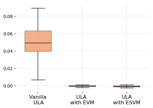
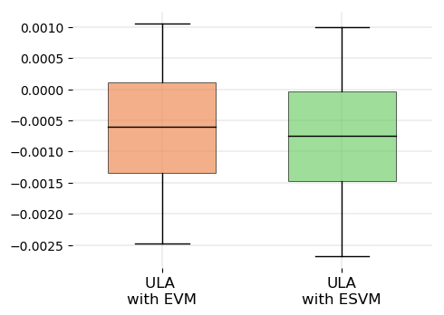
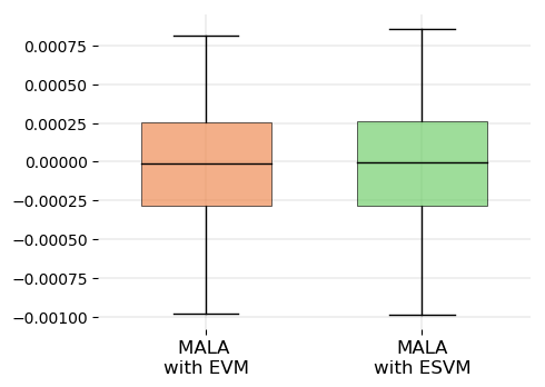
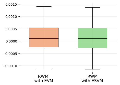
Figure 6: Estimation of $\mathsf{E}_{\pi}[X^{2}_{2}]$ in GMM with $\Sigma=\operatorname{I}$. Left figure: boxplot for ULA estimates compared to the corresponding boxplots for EVM and ESVM estimates. Next three figures: boxplots for EVM and ESVM estimates for ULA, MALA, and RWM with second-order control variates being used.

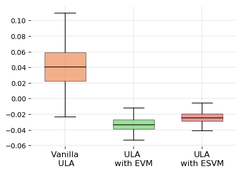
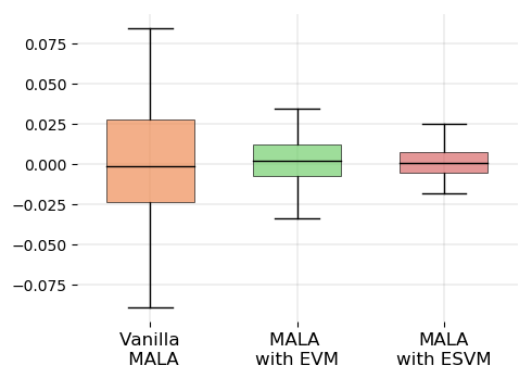
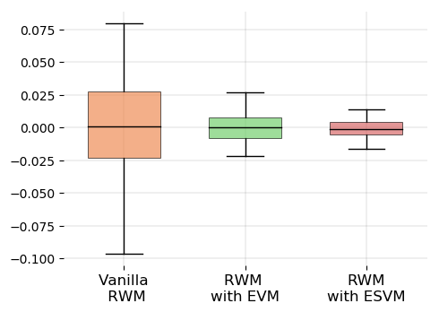
Figure 7: Estimation of $\mathsf{E}_{\pi}[X^{2}_{2}]$ in GMM with $\Sigma=\Sigma_{0}$. Left figure: boxplot for ULA estimates compared to the corresponding boxplots for EVM and ESVM estimates. Next three figures: boxplots for EVM and ESVM estimates for ULA, MALA, and RWM with second-order control variates being used.

Numerical results for estimating $\mathsf{E}_{\pi}[X_{1}]$ are presented in Table 1. The corresponding boxplots for $\mathsf{E}_{\pi}[X_{1}]$ are given in Figure 2, and for $\mathsf{E}_{\pi}[X_{1}^{2}]$ are given in Section 6, Figure 6 and Figure 7. For the sake of convenience, all the estimates are centred by their analytically computed expectations. Note that ESVM outperforms EVM in both cases $\Sigma=\operatorname{I}$ and $\Sigma=\Sigma_{0}$ and for all samplers used.

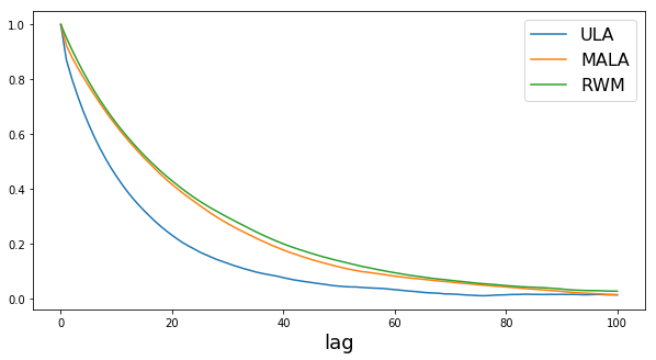
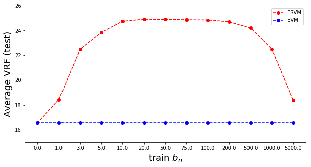
Figure 1: GMM with $\Sigma=\Sigma_{0}$. Left: Sample autocorrelation function for $X_{1}$. Right: average variance reduction factors for different choices of $b_{n}$.

Table 1: Variance Reduction Factors in GMM with $\Sigma=\operatorname{I}$ (top) and $\Sigma=\Sigma_{0}$ (bottom).

		$\mathsf{E}_{\pi}[X_{1}]$				$\mathsf{E}_{\pi}[X_{1}^{2}]$
Method		ULA	MALA	RWM		ULA	MALA	RWM
ESVM		$\mathbf{9.1}$	$\mathbf{6.1}$	$\mathbf{8.2}$		$\mathbf{609.2}$	$\mathbf{319.6}$	$\mathbf{531.2}$
EVM		$4.5$	$3.6$	$5.3$		$607.8$	$316.3$	$528.7$

		$\mathsf{E}_{\pi}[X_{1}]$				$\mathsf{E}_{\pi}[X_{1}^{2}]$
Method		ULA	MALA	RWM		ULA	MALA	RWM
ESVM		$\mathbf{24.6}$	$\mathbf{7.9}$	$\mathbf{22.2}$		$\mathbf{15.2}$	$\mathbf{9.4}$	$\mathbf{15.3}$
EVM		$16.5$	$7.5$	$14.3$		$9.2$	$5.0$	$9.3$

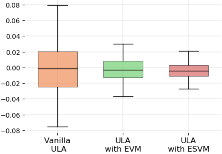
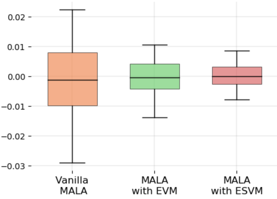
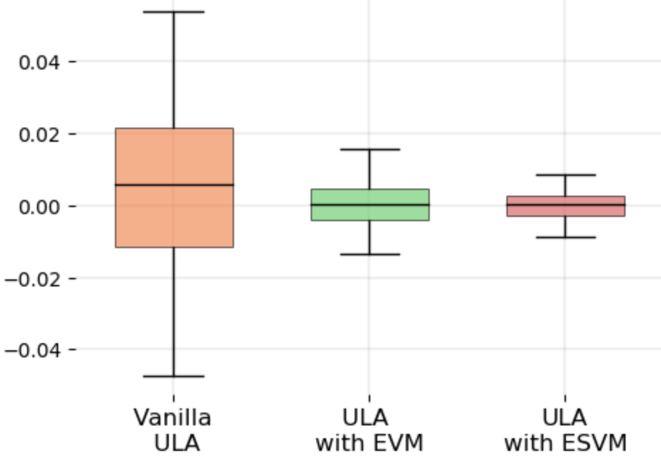
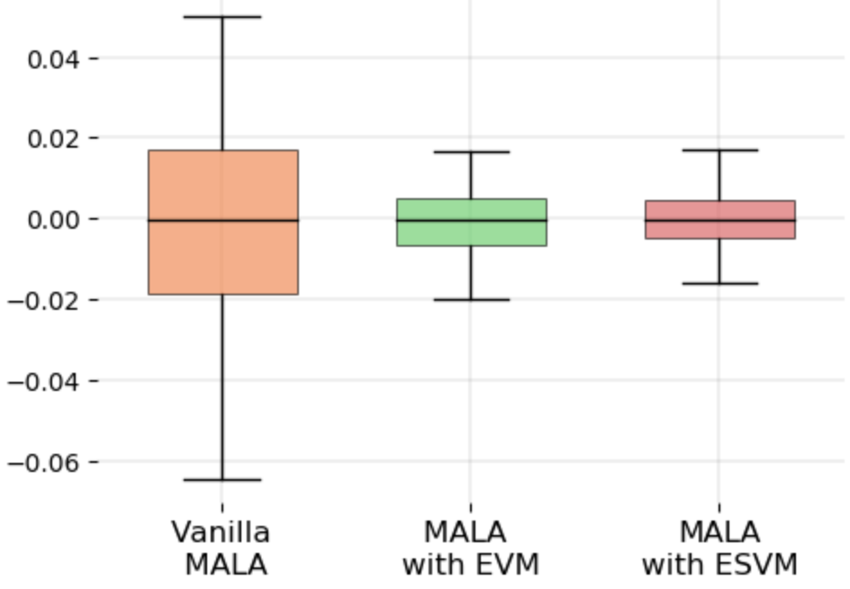
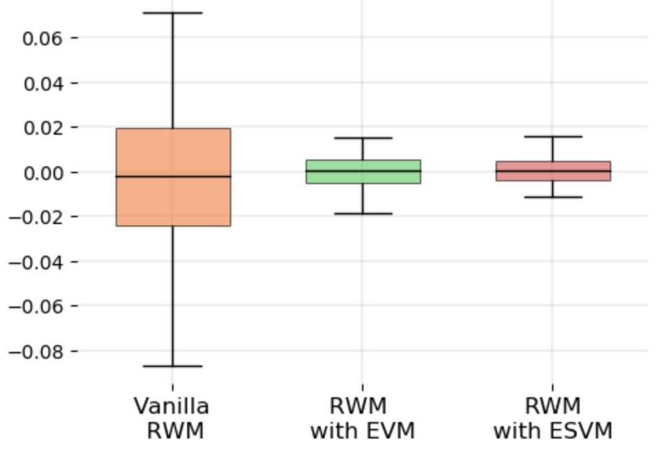
Figure 2: Estimation of $\mathsf{E}_{\pi}[X_{1}]$ in GMM with $\Sigma=\operatorname{I}$ (top row) and $\Sigma=\Sigma_{0}$ (bottom row). In each row boxplots are given for ULA, MALA, and RWM, respectively.

Gaussian Mixture with isolated modes

Let us now consider the Gaussian mixture model with different means and covariates, $\pi=\rho\mathcal{N}(\mu_{1},\sigma_{1})+(1-\rho)\mathcal{N}(-\mu_{2},\sigma_{2})$ with $\rho\in[0,1]$. For simplicity, we let $d=1$. We are interested in the case when $|\mu_{1}-\mu_{2}|\gg\max\{\sigma_{1},\sigma_{2}\}$. When sampling from $\pi$ using ULA, MALA, or RWM, the corresponding Markov chain tends to “stuck” at the modes of density $\pi$, which leads to slow convergence. We are going to compare the results obtained using ESVM and EVM with the ones from Mijatović and Vogrinc [25] based on a discretized Poisson equation. For comparison purposes, we will reproduce experiments from the aforementioned paper, see Section 5.2.1, and refer to the reported variance reduction factors.

Our aim is to estimate $\pi(f)$ with $f(x)=x^{3}$. We fix $\rho=0.4$, $\mu_{1}=-3$, $\mu_{2}=4$, $\sigma_{1}=1$, $\sigma_{2}=0.5$, and use RWM with step size $\gamma=1.0$ as a generating procedure. Results for the second-order control variates (our standard choice) are reported in Table 2, showing that this class of functions $\Phi$ does not allow us to achieve comparable to Mijatović and Vogrinc [25] variance reduction factors. Let us consider instead the following set of radial basis functions

$$\Phi(x)=\sum_{k=1}^{r}a_{k}(x-b_{k})\exp\left(-\frac{(x-b_{k})^{2}}{2}\right),$$ (19)

where $a_{k}$, $b_{k}\in\mathbb{R}$, $k=1,\ldots,r$. The ESVM algorithm with control variates determined by $\Phi(x)$ from (19) will be referred to as the ESVM-r algorithm. Results for ESVM-r are also given in Table 2 showing comparable results with the Poisson-based approach from Mijatović and Vogrinc [25] (it is referred to as the Poisson-CV) and even outperforming it for large enough train sample size $n_{\text{train}}$ and number of basis functions $r$.

Table 2: Variance Reduction Factors in GMM with isolated modes.

$n_{\text{train}}$		EVM-2	ESVM-2	Poisson-CV	ESVM-r, $r=4$	ESVM-r, $r=10$	ESVM-r, $r=20$
$10^{4}$		$1.03$	$1.04$	up to $8900$	$95.8$	$6457.2$	$265382.8$
$10^{5}$		$1.92$	$1.20$	up to $13200$	$98.8$	$7176.5$	$378249.0$

Banana-shape density

The “Banana-shape” distribution, proposed by Haario et al. [19], can be obtained from a $d$-dimensional Gaussian vector with zero mean and covariance $\mathrm{diag}(p,1,\ldots,1)$ by applying transformation

$$\varphi_{b}(x):\mathbb{R}^{d}\rightarrow\mathbb{R}^{d},\quad\varphi(x)=(x_{1},\,x_{2}+bx_{1}^{2}-pb,\,x_{3},\ldots,x_{d}),$$

where $p>0$ and $b>0$ are parameters; here $b$ controls the curvature of density’s level sets. The potential $U$ is given by

$$U(x_{1},\ldots,x_{d})=x_{1}^{2}/2p+(x_{2}+bx_{1}^{2}-pb)^{2}+\sum\nolimits_{k=3}^{d}x_{k}^{2}/2.$$

As can be easily seen, the assumption (H3) holds. As to the assumption (H1), it is fulfilled only locally. The quantity of interest is $\mathsf{E}_{\pi}[X_{2}]$. In our simulations, we set $p=100$, $b=0.1$ and consider $d=2$ and $d=8$. VRFs are reported in Table 3. Boxplots for $d=8$ are shown in Figure 3. In this problem, ESVM significantly outperforms EVM both for $d=2$ and $d=8$. Because of the curvature of the level sets, the step sizes in all considered methods should be chosen small enough, leading to highly correlated samples. This explains a poor performance of the EVM method in this context.

Table 3: Estimation of $\mathsf{E}_{\pi}[X_{2}]$ for the banana-shaped density in $d=2$ and $d=8$.

		$d=2$				$d=8$
Method		ULA	MALA	RWM		ULA	MALA	RWM
ESVM		$\mathbf{4.7}$	$\mathbf{2.7}$	$\mathbf{42.4}$		$\mathbf{5.3}$	$\mathbf{6.5}$	$\mathbf{18.5}$
EVM		$1.4$	$1.3$	$1.5$		$1.4$	$4.6$	$1.7$

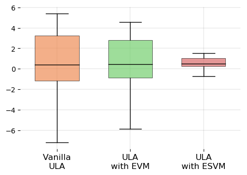
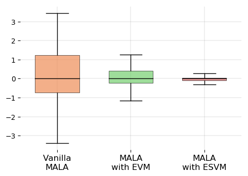
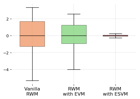
Figure 3: Estimation of $\mathsf{E}_{\pi}[X_{2}]$ for the banana-shape density in $d=8$. Boxplots are given for ULA, MALA, and RWM respectively.

Logistic and probit regression

Let $\mathsf{Y}=(\mathsf{Y}_{1},\ldots,\mathsf{Y}_{n})\in\{0,1\}^{n}$ be a vector of binary response variables, $x\in\mathbb{R}^{d}$ be a vector of regression coefficients, and $\mathsf{Z}\in\mathbb{R}^{N\times d}$ be a design matrix. The log-likelihood and likelihood of $i$-th point for the logistic and probit regression are given by

$$\IfEqCase{l}{{l}{\ell_{\operatorname{log}}}{p}{\ell_{\operatorname{pro}}}}[](\mathsf{Y}_{i}|x,\mathsf{Z}_{i}) =\mathsf{Y}_{i}\mathsf{Z}_{i}^{\top}x-\ln(1+\mathrm{e}^{\mathsf{Z}_{i}^{\top}x}),\quad\IfEqCase{l}{{l}{p_{\operatorname{log}}}{p}{p_{\operatorname{pro}}}}[](\mathsf{Y}_{i}|x,\mathsf{Z}_{i})=\exp(\IfEqCase{l}{{l}{\ell_{\operatorname{log}}}{p}{\ell_{\operatorname{pro}}}}[](\mathsf{Y}_{i}|x,\mathsf{Z}_{i})),$$

$$\IfEqCase{p}{{l}{\ell_{\operatorname{log}}}{p}{\ell_{\operatorname{pro}}}}[](\mathsf{Y}_{i}|x,\mathsf{Z}_{i}) =\mathsf{Y}_{i}\ln(\Phi(\mathsf{Z}_{i}^{\top}x))+(1-\mathsf{Y}_{i})\ln(\Phi(-\mathsf{Z}_{i}^{\top}x)),\quad\IfEqCase{p}{{l}{p_{\operatorname{log}}}{p}{p_{\operatorname{pro}}}}[](\mathsf{Y}_{i}|x,\mathsf{Z}_{i})=\exp(\IfEqCase{p}{{l}{\ell_{\operatorname{log}}}{p}{\ell_{\operatorname{pro}}}}[](\mathsf{Y}_{i}|x,\mathsf{Z}_{i})),$$

where $\mathsf{Z}_{i}^{\top}$ is the $i$-th row of $\mathsf{Z}$ for $i\in\{1,\ldots,N\}$. We complete the Bayesian model by considering the Zellner $g$-prior for the regression parameter $x$, that is, $\mathcal{N}_{d}(0,g(\mathsf{Z}^{\top}\mathsf{Z})^{-1})$. Defining $\tilde{x}=(\mathsf{Z}^{\top}\mathsf{Z})^{1/2}x$ and $\tilde{\mathsf{Z}}_{i}=(\mathsf{Z}^{\top}\mathsf{Z})^{-1/2}\mathsf{Z}_{i}$, the scalar product is preserved, that is $\langle x,\mathsf{Z}_{i}\rangle=\langle\tilde{x},\tilde{\mathsf{Z}}_{i}\rangle$ and, under the Zellner $g$-prior, $\tilde{x}\sim\mathcal{N}_{d}(0,gI_{d})$. In the sequel, we apply the algorithms in the transformed parameter space with normalized covariates and put $g=100$.

The unnormalized posterior probability distributions $\IfEqCase{l}{{g}{\pi}{l}{\pi_{\operatorname{log}}}{p}{\pi_{\operatorname{pro}}}}[]$ and $\IfEqCase{p}{{g}{\pi}{l}{\pi_{\operatorname{log}}}{p}{\pi_{\operatorname{pro}}}}[]$ for the logistic and probit regression models are defined for all $\tilde{x}\in\mathbb{R}^{d}$ by

$$\IfEqCase{l}{{g}{\pi}{l}{\pi_{\operatorname{log}}}{p}{\pi_{\operatorname{pro}}}}[](\tilde{x}|\mathsf{Y},\mathsf{Z}) \propto\exp(-\IfEqCase{l}{{l}{U_{\operatorname{log}}}{p}{U_{\operatorname{pro}}}}[](\tilde{x}))\quad\text{with}\quad\IfEqCase{l}{{l}{U_{\operatorname{log}}}{p}{U_{\operatorname{pro}}}}[](\tilde{x})=-\sum\nolimits_{i=1}^{N}\IfEqCase{l}{{l}{\ell_{\operatorname{log}}}{p}{\ell_{\operatorname{pro}}}}[](\mathsf{Y}_{i}|\tilde{x},\mathsf{Z}_{i})+(2\sigma^{2})^{-1}\left\|\tilde{x}\right\|^{2},$$

$$\IfEqCase{p}{{g}{\pi}{l}{\pi_{\operatorname{log}}}{p}{\pi_{\operatorname{pro}}}}[](\tilde{x}|\mathsf{Y},\mathsf{Z}) \propto\exp(-\IfEqCase{p}{{l}{U_{\operatorname{log}}}{p}{U_{\operatorname{pro}}}}[](\tilde{x}))\quad\text{with}\quad\IfEqCase{p}{{l}{U_{\operatorname{log}}}{p}{U_{\operatorname{pro}}}}[](\tilde{x})=-\sum\nolimits_{i=1}^{N}\IfEqCase{p}{{l}{\ell_{\operatorname{log}}}{p}{\ell_{\operatorname{pro}}}}[](\mathsf{Y}_{i}|\tilde{x},\mathsf{Z}_{i})+(2\sigma^{2})^{-1}\left\|\tilde{x}\right\|^{2}.$$

It is straightforward to check that $\IfEqCase{l}{{l}{U_{\operatorname{log}}}{p}{U_{\operatorname{pro}}}}[],\IfEqCase{p}{{l}{U_{\operatorname{log}}}{p}{U_{\operatorname{pro}}}}[]$ satisfy (LD1) and (LD2) .

We analyze the performance of ESVM algorithm on two datasets from the UCI repository. The first dataset, Pima, contains $N=768$ observations in dimension $d=9$. The second one, EEG, has dimension $d=15$, and for our experiments we take randomly selected subset of size $5000$ (to speed up sampling procedure). We split each dataset into a training part $\mathcal{T}_{N}^{\text{train}}=[(y_{i},\mathsf{Z}_{i})]_{i=1}^{N}$ and a test part $\mathcal{T}^{\text{test}}_{K}=[(y^{\prime}_{i},\mathsf{Z}^{\prime}_{i})]_{i=1}^{K}$ by randomly picking $K$ test points from the data. Then we use ULA, MALA, and RWM algorithms to sample from $\IfEqCase{l}{{g}{\pi}{l}{\pi_{\operatorname{log}}}{p}{\pi_{\operatorname{pro}}}}[](\tilde{x}|\mathsf{Y},\mathsf{Z})$ and $\IfEqCase{p}{{g}{\pi}{l}{\pi_{\operatorname{log}}}{p}{\pi_{\operatorname{pro}}}}[](\tilde{x}|\mathsf{Y},\mathsf{Z})$ respectively.

Given the sample $(\tilde{x}_{k})_{k=0}^{n-1}$, we aim at estimating the average likelihood over the test set $\mathcal{T}^{\text{test}}_{K}$, that is,

$$\int\nolimits_{\mathbb{R}^{d}}f(\tilde{x})\IfEqCase{l}{{g}{\pi}{l}{\pi_{\operatorname{log}}}{p}{\pi_{\operatorname{pro}}}}[](\tilde{x}|\mathsf{Y},\mathsf{Z})\,\mathrm{d}\tilde{x}\quad\biggl{(}\text{or }\int\nolimits_{\mathbb{R}^{d}}f(\tilde{x})\IfEqCase{p}{{g}{\pi}{l}{\pi_{\operatorname{log}}}{p}{\pi_{\operatorname{pro}}}}[](\tilde{x}|\mathsf{Y},\mathsf{Z})\,\mathrm{d}\tilde{x}\text{ for probit regression}\biggr{)},$$

where the function $f$ is given by

$$f(\tilde{x})=K^{-1}\sum_{i=1}^{K}\IfEqCase{l}{{l}{p_{\operatorname{log}}}{p}{p_{\operatorname{pro}}}}[](y^{\prime}_{i}|\mathsf{Z}^{\prime}_{i},\tilde{x})\quad\biggl{(}\text{or }K^{-1}\sum_{i=1}^{K}\IfEqCase{p}{{l}{p_{\operatorname{log}}}{p}{p_{\operatorname{pro}}}}[](y^{\prime}_{i}|\mathsf{Z}^{\prime}_{i},\tilde{x})\text{ for probit regression}\biggr{)}.$$

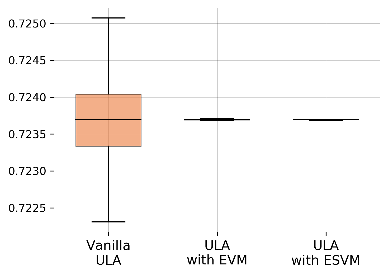
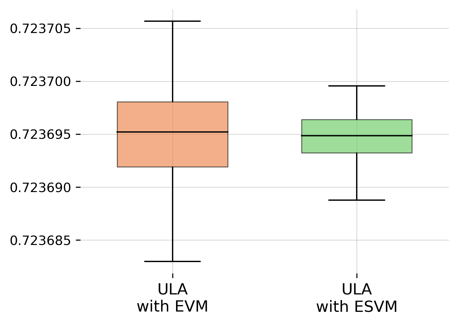
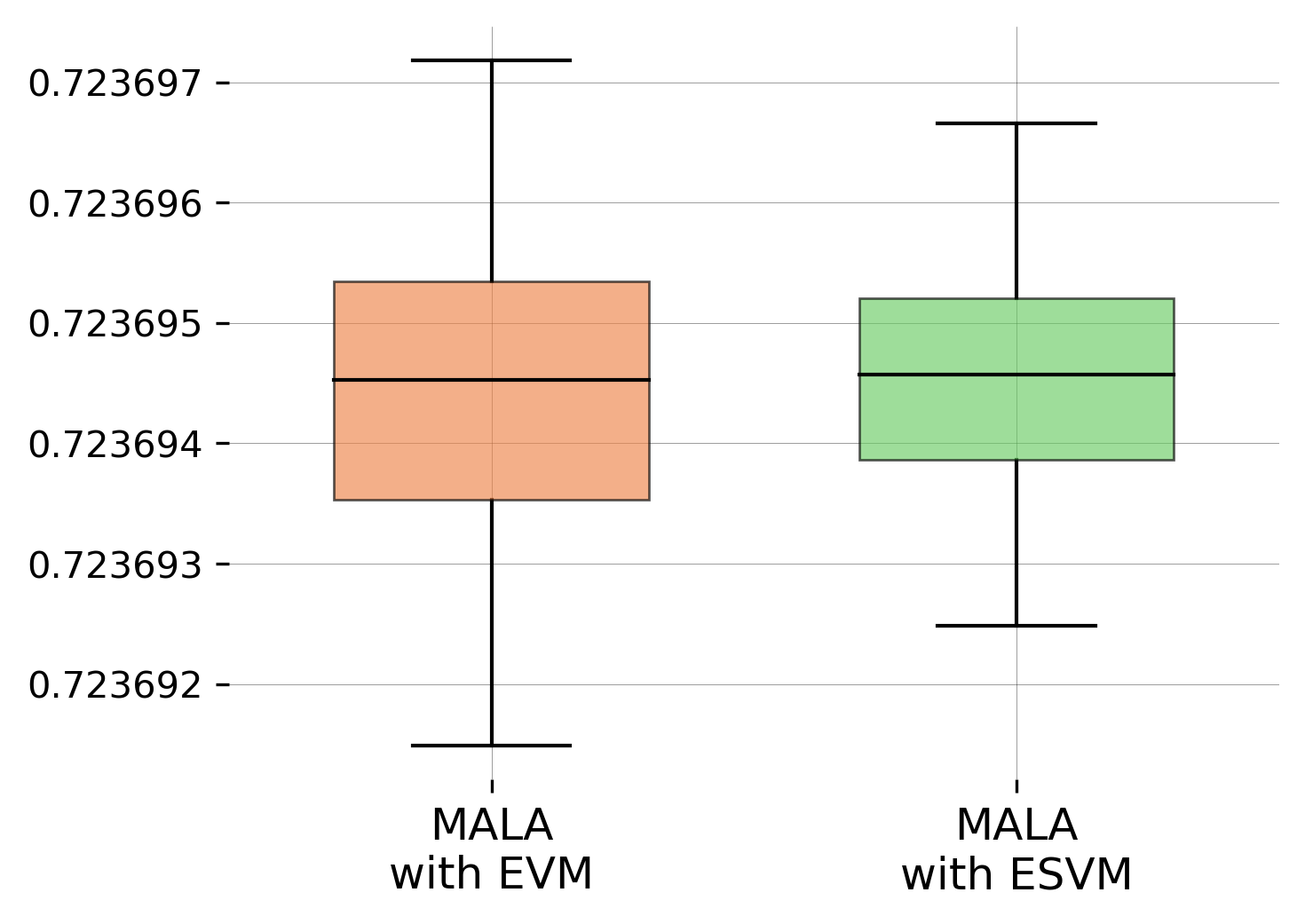
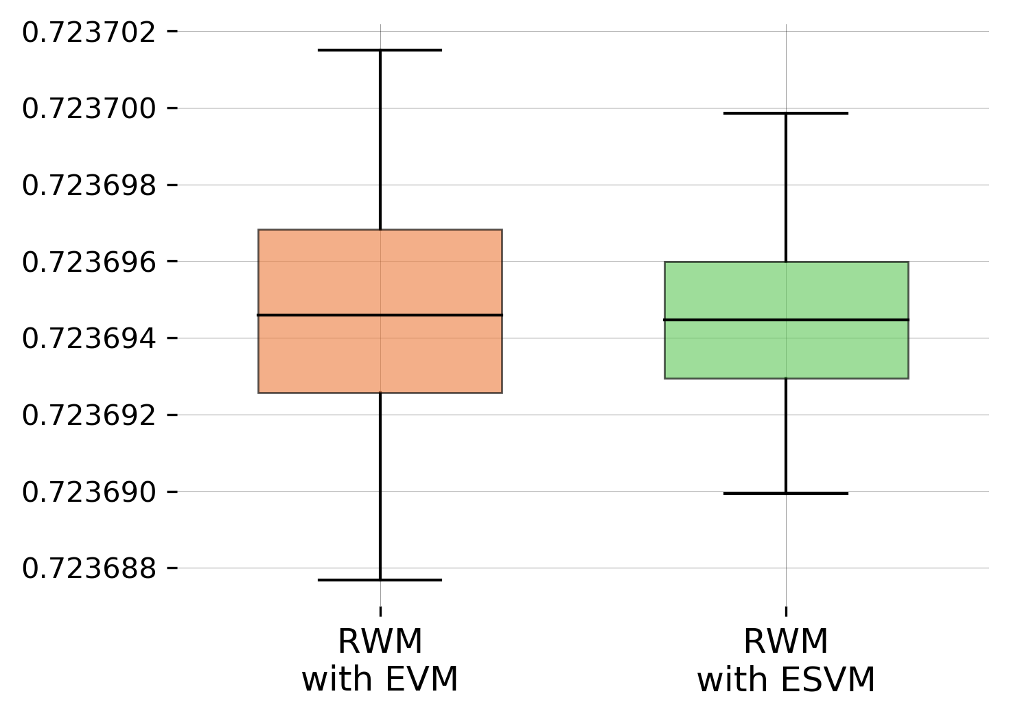
Figure 8: Estimation of the average test likelihood in probit regression for the Pima dataset. Left figure: boxplot for ULA estimates compared to the corresponding boxplots for EVM and ESVM estimates. Next three figures: boxplots for EVM and ESVM estimates for ULA, MALA, and RWM with second-order control variates being used.

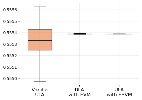
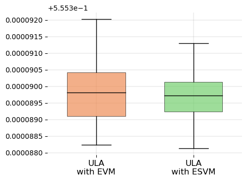
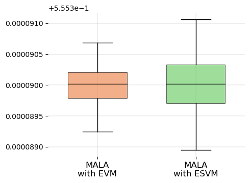
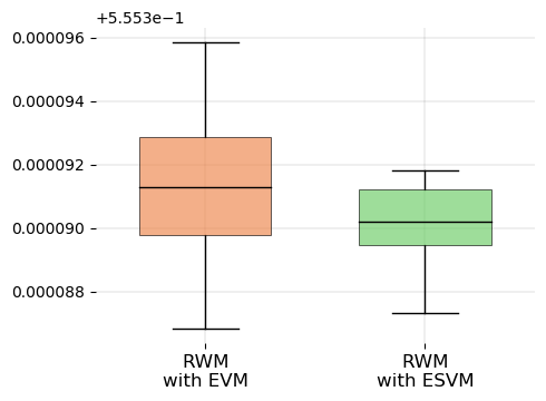
Figure 9: Estimation of the average test likelihood in probit regression for the EEG dataset. Left figure: boxplot for ULA estimates compared to the corresponding boxplots for EVM and ESVM estimates. Next three figures: boxplots for EVM and ESVM estimates for ULA, MALA, and RWM with second-order control variates being used.

VRFs are reported for first- and second-order control variates. Results for logistic regression are given in Table 4. Boxplots for the average test likelihood estimation using second-order control variates are shown in Figure 4. The same quantities for probit regression are reported in Section 6, see Table 7, Figure 8, and Figure 9.

Note that ESVM also outperforms EVM in this example. It is worth noting that for ULA and RWM, we show up to $100$ times better performance in terms of VRF. For MALA, the results for EVM and ESVM are similar since the samples are much less positively correlated.

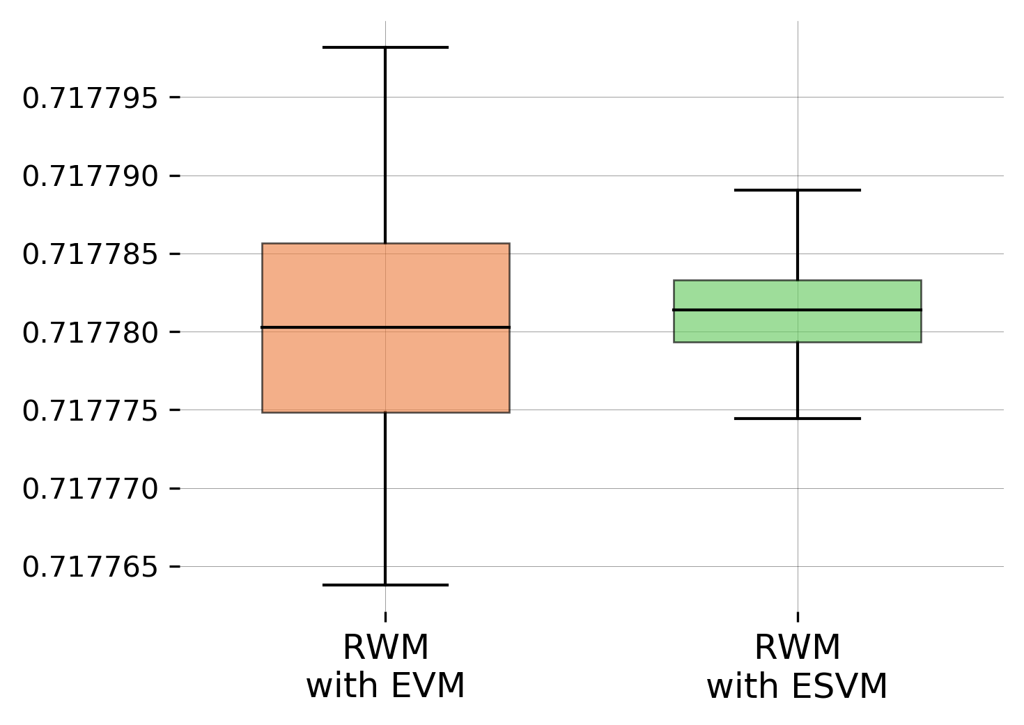
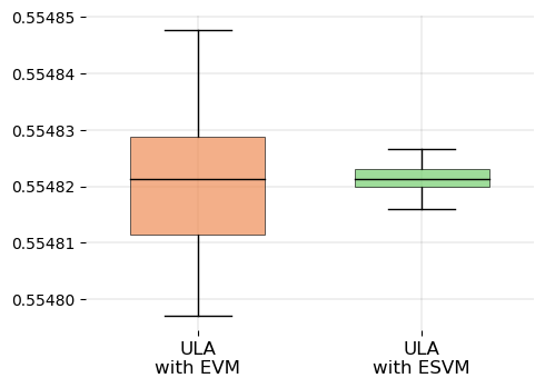
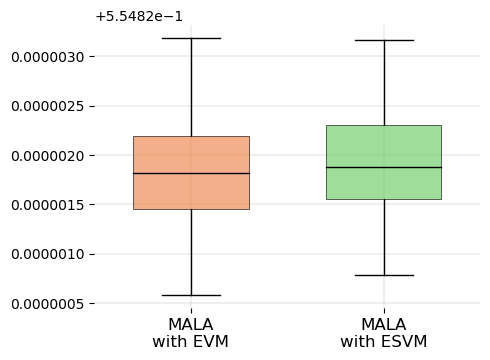
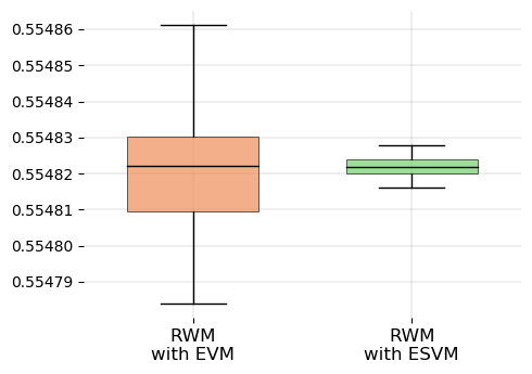
Figure 4: Estimation of the average test likelihood in logistic regression for the Pima dataset (top row) and the EEG dataset (bottom row). In each row boxplots are given for ULA, MALA, and RWM respectively.

Table 4: Average test likelihood estimation in logistic regression.

		PIMA dataset				EEG dataset
Method		ULA	MALA	RWM		ULA	MALA	RWM
ESVM-1		$347.6$	$535.6$	$411.7$		$542.3$	$996.6$	$483.5$
EVM-1		$347.9$	$542.1$	$415.5$		$548.1$	$1020.2$	$508.9$
ESVM-2		$\mathbf{11387.3}$	$\mathbf{28792.8}$	$\mathbf{19503.3}$		$\mathbf{11406.6}$	$\mathbf{44612.5}$	$\mathbf{11324.9}$
EVM-2		$2704.8$	$4087.3$	$5044.1$		$350.3$	$39985.4$	$453.3$

Van der Pol oscillator equation

The setup of this experiment is much similar to the one reported in South et al. [37]. Here a position $p_{x}(t)\in\mathbb{R}$ evolves in time $t$ according to the second order differential equation

$$\frac{\mathrm{d}^{2}p_{x}}{\mathrm{d}t^{2}}-x(1-p_{x}^{2})\frac{\mathrm{d}p_{x}}{\mathrm{d}t}+p=0,$$ (20)

where $x\in\mathbb{R}$ is an unknown parameter indicating the non-linearity and the strength of the damping. Letting $q_{x}=\mathrm{d}p_{x}/\mathrm{d}t$ we can formulate the oscillator as the first-order system

$$\begin{cases}\frac{\mathrm{d}p_{x}}{\mathrm{d}t}=q_{x},\\ \frac{\mathrm{d}q_{x}}{\mathrm{d}t}=x(1-p_{x}^{2})q_{x}+p_{x},\end{cases}$$

where only the first component $p_{x}$ is observed. This system was solved numerically using $x_{\star}=1$ and starting point $p_{x_{\star}}(0)=0$, $q_{x_{\star}}(0)=2$. Observations $\mathsf{Y}_{i}=p_{x_{\star}}(t_{i})+\varepsilon_{i}$ were made at successive time instants $t_{i}=i$, $i=1,\ldots,T$, and Gaussian measurement noise $\varepsilon_{i}$ of standard deviation $\sigma=0.5$ was added. We use a normal prior $\pi_{0}(x)$ with mean $\mu=1$ and standard deviation $\sigma_{0}=0.5$. The unnormalized posterior probability distribution is defined for all $x>0$ by

$$\pi(x|\mathsf{Y}) \propto\exp(-U(x))\quad\text{with}\quad U(x)=-\log\pi_{0}(x)+\sum_{i=1}^{T}\frac{(\mathsf{Y}_{i}-p_{x}(t_{i}))^{2}}{2\sigma^{2}}.$$

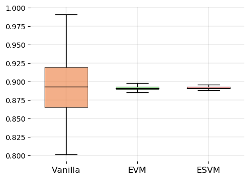
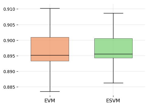
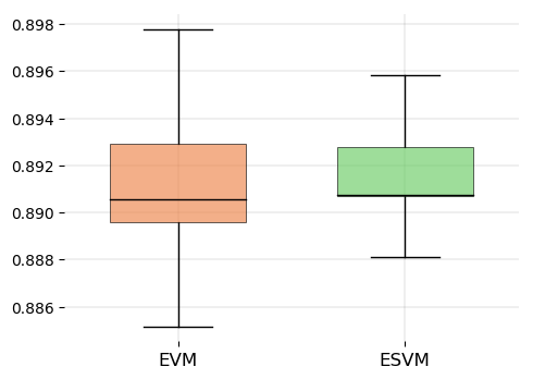
Figure 10: Estimating the mean of the posterior distribution in the Van der Pol model. From left to right: boxplots for vanilla estimates and the corresponding EVM and ESVM estimates with third-order polynomials being used as control variates, EVM and ESVM comparison for second-order polynomials, and EVM and ESVM comparison for third-order polynomials.

Clearly, $U$ satisfies (LD1) and (LD3) . To sample from $\pi(x|\mathsf{Y})$ we use the MALA algorithm. The quantity of interest is the posterior mean $\int\nolimits_{\mathbb{R}}x\pi(x|\mathsf{Y})\,\mathrm{d}x$. In this example, we use control variates up to degree $3$. Results are presented in Section 6 — VRFs are summarized in Table 8 and boxplots for the second-order control variates are given in Figure 10. In this problem, ESVM slightly outperforms EVM in terms of variance reduction factor.

Lotka-Volterra system

The Lotka-Volterra model is a well-known system of ODEs describing the joint evolution of two interacting biological populations, predators and preys. Denote the population of preys and predators at moment $t$ by $u(t)$ and $v(t)$ respectively, then the corresponding model can be written as the following first-order system

$$\begin{cases}\frac{\mathrm{d}u}{\mathrm{d}t}=(\alpha-\beta v)u,\\ \frac{\mathrm{d}v}{\mathrm{d}t}=(-\gamma+\delta u)v,\\ u(0)=u_{0},\ v(0)=v_{0}.\end{cases}$$ (21)

The parameter vector is given by $x=(\alpha,\beta,\gamma,\delta)$, with all components being non-negative due to the physical meaning of the problem. The system was solved numerically with the true parameters $x_{\star}=(0.6,0.025,0.8,0.025)$ and starting populations $u_{0}=30.0$, $v_{0}=4.0$. The system is observed at successive time moments $t_{i}=i$, $i=1,\ldots,T$, with the lognormal measurements $\mathsf{Y}_{i}\sim\operatorname{Lognormal}(\log{u(t_{i})},\sigma^{2})$, $\mathsf{Z}_{i}\sim\operatorname{Lognormal}(\log{v(t_{i})},\sigma^{2})$ with $\sigma=0.25$. A weakly informative normal prior $\pi_{0}(x)$ was used for the model parameters: $\mathcal{N}(1,0.5)$ for $\alpha$ and $\gamma$, $\mathcal{N}(0.05,0.05)$ for $\beta$ and $\delta$. The posterior distribution is given by $\pi(x|\mathsf{Y},\mathsf{Z})\propto\exp(-U(x))$, where

$$U(x)=-\log\pi_{0}(x)+\sum_{i=1}^{T}\biggl{(}\frac{(\log{\mathsf{Y}_{i}}-\log{u(t_{i})})^{2}+(\log{\mathsf{Z}_{i}}-\log{v(t_{i})})^{2}}{2\sigma^{2}}+\log{\mathsf{Y}_{i}}+\log{\mathsf{Z}_{i}}\biggr{)}.$$

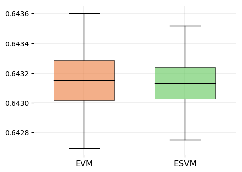
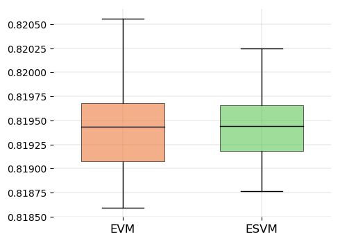
Figure 11: Estimating the mean of the posterior distribution in the Lotka-Volterra model. From left to right: posterior mean for parameters $\alpha,\beta,\gamma$, and $\delta$.

We use the MALA algorithm to sample from $\pi(x|\mathsf{Y},\mathsf{Z})$. The quantity of interest is the posterior mean $\int\nolimits_{\mathbb{R}^{4}}x\pi(x|\mathsf{Y},\mathsf{Z})\,\mathrm{d}x$. VRFs are summarized in Table 5 and boxplots for the second-order control variates are given in Figure 5 and Section 6, Figure 11. For some model parameters ESVM significantly outperforms EVM in terms of VRF, for others the results are comparable with slight superiority of ESVM.

Table 5: Estimation of the posterior mean in the Lotka-Volterra model.

Estimated parameter		$\alpha$	$\beta$	$\delta$	$\gamma$
ESVM-1		$\mathbf{10.5}$	$\mathbf{6.5}$	$\mathbf{6.2}$	$\mathbf{8.3}$
EVM-1		$6.6$	$4.2$	$4.9$	$6.0$
ESVM-2		$\mathbf{757.6}$	$\mathbf{427.8}$	$\mathbf{277.2}$	$\mathbf{446.6}$
EVM-2		$642.1$	$286.0$	$275.0$	$429.7$

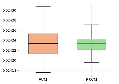
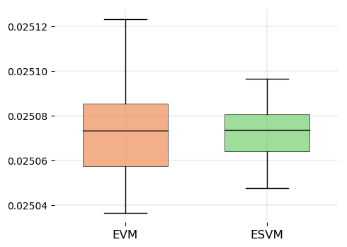
Figure 5: Estimation of the posterior mean of $\beta$ (left figure) and $\delta$ (right figure) in the Lotka-Volterra model.

5 Proofs

5.1 Proof of Section 2.2

Before we proceed to the proof of Section 2.2, let us refer to a general result from Nickl and Pötscher [27] which is used below to bound the fixed point of a subset of a weighted Sobolev space. First we need to introduce some notations.

Let $\mu$ be a (nonnegative) Borel measure. Given the two functions $l,u:\mathsf{X}\to\mathbb{R}$ in $\mathrm{L}^{p}(\mu)$, the bracket $[l,u]$ is the set of all functions in $\mathrm{L}^{p}(\mu)$ with $l\leq f\leq u$. The $\mathrm{L}^{p}(\mu)$-size of the bracket $[l,u]$ is defined as $\|l-u\|_{\mathrm{L}^{p}(\mu)}$. The $\mathrm{L}^{p}(\mu)$-bracketing number $\mathcal{N}^{[\,]}_{\mathrm{L}^{p}(\mu)}(F,\varepsilon)$ of a (non-empty) set $F$ is the minimal number of brackets of $\mathrm{L}^{p}(\mu)$-size less than or equal to $\varepsilon>0$ necessary to cover $F$. The logarithm of the bracketing number is called the $\mathrm{L}^{p}(\mu)$-bracketing metric entropy $H^{[\,]}_{\mathrm{L}^{p}(\mu)}(F,\varepsilon)$.

Theorem 3 ([27, Corollary 4])

Let $1<p<\infty$, $\beta\in\mathbb{R}$, and $s-d/p>0$. Let $F$ be a (non-empty) norm-bounded subset of $W^{s,p}(\mathbb{R}^{d},\langle x\rangle^{\beta})$. Suppose $M$ is a (non-empty) family of Borel measures on $\mathbb{R}^{d}$ such that the condition $\sup_{\mu\in M}\|\langle x\rangle^{\alpha-\beta}\|_{L^{r}(\mu)}<\infty$ holds for some $1\leq r\leq\infty$ and for some $\alpha>0$. Then

$$\sup_{\mu\in M}H^{[\,]}_{L^{r}(\mu)}(F,\varepsilon)\lesssim\begin{cases}\varepsilon^{-d/s}&\text{for }\alpha>s-d/p,\\ \varepsilon^{-(\alpha/d+1/p)^{-1}}&\text{for }\alpha<s-d/p.\\ \end{cases}$$

• We first bound the metric entropy of $\mathcal{H}$ by the bracketing metric entropy. If $h\in\mathcal{H}$ is in the $2\varepsilon$-bracket $[l,u]$, $l,u\in\mathcal{H}$, then it is in the ball of radius $\varepsilon$ around $(l+u)/2$. So,

  $$H_{\mathrm{L}^{2}(\pi)}(\mathcal{H},\varepsilon)\leq H^{[\,]}_{\mathrm{L}^{2}(\pi)}(\mathcal{H},2\varepsilon).$$

  Now our aim is apply Theorem 3 to $\mathcal{H}$ which is a norm-bounded subset of $W^{s,p}(\mathbb{R}^{d},\langle x\rangle^{\beta})$ by assumption. For $M=\{\pi\}$ and $r=2$, the condition $\sup_{\mu\in M}\|\langle x\rangle^{\alpha-\beta}\|_{L^{r}(\mu)}<\infty$ also holds by assumption. Hence,

  $$H_{\mathrm{L}^{2}(\pi)}(\mathcal{H},\varepsilon)\lesssim\begin{cases}\varepsilon^{-d/s}&\text{for }\alpha>s-d/p,\\ \varepsilon^{-(\alpha/d+1/p)^{-1}}&\text{for }\alpha<s-d/p.\\ \end{cases}$$

  Now we turn to the bound for the fixed point $\gamma_{\mathrm{L}^{2}(\pi)}(\mathcal{H},n)$ (see (9)). Consider first the case $\alpha>s-d/p$. The solution to the inequality $\varepsilon^{-d/s}\lesssim n\varepsilon^{2}$ is $\varepsilon\gtrsim n^{-\frac{1}{2+d/s}}$. Taking $\varepsilon_{0}\sim n^{-\frac{1}{2+d/s}}$, where $\sim$ stands for equality up to a constant, yields

  $$H_{\mathrm{L}^{2}(\pi)}(\mathcal{H},\varepsilon_{0})\lesssim n\varepsilon_{0}^{2},\quad\text{for }\alpha>s-d/p.$$

  Since $\gamma_{\mathrm{L}^{2}(\pi)}(\mathcal{H},n)$ is the infimum over all such $\varepsilon>0$, it holds $\gamma_{\mathrm{L}^{2}(\pi)}(\mathcal{H},n)\lesssim n^{-\frac{1}{2+d/s}}$. Repeated computations for $\alpha<s-d/p$ give us $\gamma_{\mathrm{L}^{2}(\pi)}(\mathcal{H},n)\lesssim n^{-\frac{1}{2+(\alpha/d+1/p)^{-1}}}$. Combining these two bounds, we have

  $$\gamma_{\mathrm{L}^{2}(\pi)}(\mathcal{H},n)\lesssim\begin{cases}n^{-\frac{1}{2+d/s}}&\text{for }\alpha>s-d/p,\\ n^{-\frac{1}{2+(\alpha/d+1/p)^{-1}}}&\text{for }\alpha<s-d/p,\\ \end{cases}$$

  which is the desired conclusion. $\square$

5.2 Spectral variance estimator

We investigate properties of the spectral variance ${V}_{n}(h)$ defined in (5). Note that ${V}_{n}(h)$ can be represented as a quadratic form $Z_{n}(h)^{\top}A_{n}Z_{n}(h)$, where $Z_{n}(h)=(h(X_{0}),\ldots,h(X_{n-1}))^{\top}$ and $A_{n}$ is an $n\times n$ symmetric matrix. Namely, let $\operatorname{I}_{n}$ be the identity $n\times n$ matrix and ${1}_{n}=(1,\dots,1)^{\top}\in\mathbb{R}^{n}$. Given the lag window $w_{n}$, we denote the weight matrix by $W_{n}=(w_{n}(j-i))_{i,j=1}^{n}$. By rearranging the summations in (5), we have

$${V}_{n}(h)=n^{-1}\sum_{k=0}^{n-1}\sum_{j=0}^{n-1}w_{n}(k-j)\Bigl{(}h(X_{k})-\pi_{n}(h)\Bigr{)}\Bigl{(}h(X_{j})-\pi_{n}(h)\Bigr{)},$$

Hence the spectral variance can be represented as

$${V}_{n}(h)=Z_{n}(h)^{\top}A_{n}Z_{n}(h)\quad\text{for}\ A_{n}=\frac{1}{n}\,\left(\operatorname{I}_{n}-\frac{1}{n}{1}_{n}{1}_{n}^{\top}\right)^{\top}W_{n}\left(\operatorname{I}_{n}-\frac{1}{n}{1}_{n}{1}_{n}^{\top}\right).$$ (22)

In the following lemma we provide an upper bound on the operator norm of $A_{n}$.

Lemma

If the truncation point $b_{n}$ of the lag window $w_{n}$ satisfies $b_{n}\leq n$, then $\left\|A_{n}\right\|\leq 2{b_{n}}/{n}$.

• Denote $P=\operatorname{I}_{n}-n^{-1}{1}_{n}{1}_{n}^{\top}$. Since $P$ is an orthonormal projector, we get

  $$\left\|A_{n}\right\|=\frac{1}{n}\|PW_{n}P\|\leq\frac{1}{n}\|W_{n}\|.$$

  To bound the operator norm of $W_{n}$ (which is a Toeplitz matrix), we use the standard technique based on the discrete-time Fourier transform of the sequence $w:[-b_{n},b_{n}]\to[0,1]$, defined, for $\lambda\in[-\pi,\pi)$ by

  $$\hat{w}_{n}(\lambda)=\sum_{k=-b_{n}}^{b_{n}}w_{n}(k)\mathrm{e}^{-\mathrm{i}k\lambda}\,.$$

  Obviously, $|\hat{w}_{n}(\lambda)|\leq 2b_{n}$. We have $\|W_{n}\|=\sup_{\|x\|=1}x^{\top}W_{n}x$. Moreover, for any unit vector $u=(u_{1},\ldots,u_{n})^{\top}$ it holds

  $$u^{\top}W_{n}u =\sum_{k,j=1}^{n}\left(\frac{1}{2\pi}\int_{-\pi}^{\pi}\mathrm{e}^{\mathrm{i}(k-j)\lambda}\hat{w}_{n}(\lambda)\mathrm{d}\lambda\right)u_{k}u_{j}=\frac{1}{2\pi}\int_{-\pi}^{\pi}\biggl{|}\sum_{k=1}^{n}\mathrm{e}^{\mathrm{i}k\lambda}u_{k}\biggr{|}^{2}\hat{w}_{n}(\lambda)\mathrm{d}\lambda\leq 2b_{n}.$$

  Hence $\|W_{n}\|\leq 2b_{n}$ and $\|A_{n}\|\leq 2b_{n}/n$. The lemma is proved. $\square$

In the next lemma we prove several technical results on expectation of the operator norm of $Z_{n}(h)$ and ${V}_{n}(h)$ which hold under (GE) assumption.

Lemma

Under (GE) , it holds for any $h,h^{\prime}\in\mathcal{H}$

$$\mathsf{E}_{x_{0}}\Bigl{[}\|Z_{n}(h)\|^{2}\Bigr{]}\leq n\|h\|_{\mathrm{L}^{2}(\pi)}^{2}+\frac{\varsigma W(x_{0})}{1-\rho}\|h\|^{2}_{W^{1/2}},$$

and

$$\mathsf{E}_{x_{0}}\Bigl{[}\|Z_{n}(h)-Z_{n}(h^{\prime})\|^{2}\Bigr{]} \leq n\|h-h^{\prime}\|_{\mathrm{L}^{2}(\pi)}^{2}+\frac{\varsigma W(x_{0})}{1-\rho}\|h-h^{\prime}\|^{2}_{W^{1/2}}.$$

Moreover, for any $h\in\mathcal{H}$, this bound implies

$$\mathsf{E}_{x_{0}}\big{[}{V}_{n}(h)\big{]}\leq 2b_{n}{\|h\|_{\mathrm{L}^{2}(\pi)}^{2}}+\frac{2\|h\|^{2}_{W^{1/2}}\varsigma W(x_{0})}{1-\rho}\frac{b_{n}}{n}.$$

• We first observe that

  $$\mathsf{E}_{x_{0}}\Bigl{[}\|Z_{n}(h)\|^{2}\Bigr{]}=\mathsf{E}_{x_{0}}\left[\sum\nolimits_{k=0}^{n-1}h^{2}(X_{k})\right]=\sum\nolimits_{k=0}^{n-1}\|h\|_{\mathrm{L}^{2}(P^{k}(x_{0},\cdot))}^{2}.$$

  Now each summand can be bounded in the following way,

  $$\|h\|_{\mathrm{L}^{2}(P^{k}(x_{0},\cdot))}^{2} =\|h\|_{\mathrm{L}^{2}(\pi)}^{2}+\Bigl{(}\|h\|_{\mathrm{L}^{2}(P^{k}(x_{0},\cdot))}^{2}-\|h\|_{\mathrm{L}^{2}(\pi)}^{2}\Bigr{)}$$

  $$\leq\|h\|_{\mathrm{L}^{2}(\pi)}^{2}+\int|h(x)|^{2}|P^{k}(x_{0},\cdot)-\pi|(\mathrm{d}x)$$

  $$\leq\|h\|_{\mathrm{L}^{2}(\pi)}^{2}+\|h\|_{{W^{1/2}}}^{2}\|P^{k}(x_{0},\cdot)-\pi\|_{{W}}.$$

  This inequality and (GE) together imply

  $$\mathsf{E}_{x_{0}}\Bigl{[}\|Z_{n}(h)\|^{2}\Bigr{]} \leq n\|h\|_{\mathrm{L}^{2}(\pi)}^{2}+\frac{\|h\|^{2}_{W^{1/2}}\varsigma W(x_{0})}{1-\rho}\,,$$

  which proves the first inequality. Repeated computations for $Z_{n}(h)-Z_{n}(h^{\prime})$ yield

  $$\mathsf{E}_{x_{0}}\Bigl{[}\|Z_{n}(h)-Z_{n}(h^{\prime})\|^{2}\Bigr{]} \leq n\|h-h^{\prime}\|_{\mathrm{L}^{2}(\pi)}^{2}+\frac{\varsigma W(x_{0})}{1-\rho}\|h-h^{\prime}\|^{2}_{W^{1/2}}.$$

  The first statement is proved. To prove the second statement we note that

  $$\mathsf{E}_{x_{0}}\big{[}{V}_{n}(h)\big{]}=\mathsf{E}_{x_{0}}\Bigl{[}Z_{n}(h)^{\top}A_{n}Z_{n}(h)\Bigr{]}\leq\|A_{n}\|\mathsf{E}_{x_{0}}\Bigl{[}\|Z_{n}(h)\|^{2}\Bigr{]}.$$

  By Section 5.2 we have $\|A_{n}\|\leq 2b_{n}/n$. Substituting this we deduce our claim. $\square$

It is known that the spectral variance ${V}_{n}(h)$ is a biased estimate of the asymptotic variance ${V}_{\infty}(h)$. In the following proposition we show how close is the expected value of ${V}_{n}(h)$ to ${V}_{\infty}(h)$.

Proposition

Assume (GE) . Then for any $h\in\mathcal{H}$ and any $x_{0}\in\mathsf{X}$,

$$\Bigl{|}\mathsf{E}_{x_{0}}\big{[}{V}_{n}(h)\big{]}-V_{\infty}(h)\Bigr{|}\leq\frac{\varsigma^{1/2}\pi(W)\|\tilde{h}\|_{{W^{1/2}}}^{2}}{1-\rho^{1/2}}\biggl{(}\frac{9\varsigma W(x_{0})}{(1-\rho)\pi(W)}\frac{b_{n}}{n^{2}}+\frac{9b_{n}}{n}+2\rho^{b_{n}/2}\biggr{)}\,,$$

where $\tilde{h}=h-\pi(h)$. Moreover, if $n\geq\varsigma W(x_{0})/((1-\rho)\pi(W))$ then

$$\Bigl{|}\mathsf{E}_{x_{0}}\big{[}{V}_{n}(h)\big{]}-V_{\infty}(h)\Bigr{|}\leq\frac{20\varsigma^{1/2}\pi(W)\|\tilde{h}\|_{{W^{1/2}}}^{2}}{1-\rho^{1/2}}\biggl{(}\frac{b_{n}}{n}\vee\rho^{b_{n}/2}\biggr{)}\,,$$

where $a\vee b\overset{\text{\tiny def}}{=}\max\{a,b\}$.

• Recall that the asymptotic variance ${V}_{\infty}(h)$ may be written as ${V}_{\infty}(h)=\sum_{|s|\geq 0}\rho_{\pi}^{(h)}(|s|)$ with $\rho_{\pi}^{(h)}(s)=\mathsf{E}_{\pi}\big{[}\tilde{h}(X_{0})\tilde{h}(X_{s})\big{]}$ and, by definition, ${V}_{n}(h)=\sum_{|s|<b_{n}}w_{n}(s)\hat{\rho}_{n}^{(h)}(|s|)\,$, where the lag $s$ empirical autocovariance coefficient $\hat{\rho}_{n}^{(h)}(s)$ is given in (4). We have

  $$\Bigl{|}\mathsf{E}_{x_{0}}\big{[}{V}_{n}(h)\big{]}-V_{\infty}(h)\Bigr{|} \leq 2\sum_{s=0}^{b_{n}-1}w_{n}(s)\bigl{|}\mathsf{E}_{x_{0}}\big{[}\hat{\rho}_{n}^{(h)}(s)\big{]}-\rho_{\pi}^{(h)}(s)\bigr{|}$$

  $$\qquad\qquad\qquad+2\sum_{s=0}^{b_{n}-1}|1-w_{n}(s)||\rho_{\pi}^{(h)}(s)|+2\sum_{s=b_{n}}^{\infty}|\rho_{\pi}^{(h)}(s)|\,.$$ (23)

  To bound each summand in this decomposition, we need the following lemma.

  Lemma

  Assume (GE) . Then for any $h\in\mathcal{H}$, $x\in\mathcal{X}$, and $s\in\mathbb{Z}_{+}$,

  $$\Bigl{|}\mathsf{E}_{x}\big{[}\tilde{h}(X_{0})\tilde{h}(X_{s})\big{]}\Bigr{|}\leq\varsigma^{1/2}\rho^{s/2}W(x)\|\tilde{h}\|_{{W^{1/2}}}^{2}\,,$$ (24)

  and

  $$\bigr{|}\rho_{\pi}^{(\tilde{h})}(s)\bigl{|}\leq\varsigma^{1/2}\rho^{s/2}\pi(W)\|\tilde{h}\|_{{W^{1/2}}}^{2}\,.$$ (25)

  • The proof is straightforward. Since $\pi(\tilde{h})=0$, we have

    $$\Bigl{|}\mathsf{E}_{x}\big{[}\tilde{h}(X_{0})\tilde{h}(X_{s})\big{]}\Bigr{|} \leq\bigl{|}\tilde{h}(x)\bigr{|}\biggl{|}\int_{\mathsf{X}}\tilde{h}(y)\bigl{(}P^{s}(x,\cdot)-\pi\bigr{)}(\mathrm{d}y)\biggr{|}$$

    $$\leq\|\tilde{h}\|_{{W^{1/2}}}^{2}W^{1/2}(x)\int_{\mathsf{X}}W^{1/2}(y)\bigl{|}P^{s}(x,\cdot)-\pi\bigr{|}(\mathrm{d}y)\,.$$

    By Hölder’s inequality,

    $$\int_{\mathsf{X}}W^{1/2}(y)\bigl{|}P^{s}(x,\cdot)-\pi\bigr{|}(\mathrm{d}y) \leq\bigl{|}P^{s}(x,\mathsf{X})-\pi(\mathsf{X})\bigr{|}^{1/2}\biggl{(}\int_{\mathsf{X}}W(y)\bigl{|}P^{s}(x,\cdot)-\pi\bigr{|}(\mathrm{d}y)\biggr{)}^{1/2}$$

    $$\leq\|P^{s}(x,\cdot)-\pi\|_{{W}}^{1/2}\,.$$

    Combining these bounds and using (GE) , we conclude

    $$\Bigl{|}\mathsf{E}_{x}\big{[}\tilde{h}(X_{0})\tilde{h}(X_{s})\big{]}\Bigr{|} \leq\varsigma^{1/2}\rho^{s/2}W(x)\|\tilde{h}\|_{{W^{1/2}}}^{2}\,,$$

    and (24) is proved. Integrating this relation with respect to the stationary distribution $\pi$, we obtain the second inequality. The lemma is proved. $\square$

  Let us first bound the last two summands in the decomposition (23). By definition, $w_{n}(s)=1$ for all $s\in[-b_{n}/2,b_{n}/2]$. From (25) we have the second summand

  $$\sum_{s=0}^{b_{n}-1}|1-w_{n}(s)||\rho_{\pi}^{(h)}(s)| \leq\sum_{s=\lceil{b_{n}/2}\rceil}^{b_{n}-1}|\rho_{\pi}^{(h)}(s)|\leq\varsigma^{1/2}\pi(W)\|\tilde{h}\|_{{W^{1/2}}}^{2}\frac{\rho^{b_{n}/2}}{1-\rho^{1/2}}\,.$$ (26)

  where $\lceil{b_{n}/2}\rceil$ is the nearest integer greater than or equal to $b_{n}/2$. Similar arguments apply to the last summand in (23),

  $$\sum_{s=b_{n}}^{\infty}|\rho_{\pi}^{(h)}(s)|\leq\varsigma^{1/2}\pi(W)\|\tilde{h}\|_{{W^{1/2}}}^{2}\frac{\rho^{b_{n}}}{1-\rho^{1/2}}\leq\varsigma^{1/2}\pi(W)\|\tilde{h}\|_{{W^{1/2}}}^{2}\frac{\rho^{b_{n}/2}}{1-\rho^{1/2}}\,.$$ (27)

  It remains to bound the first summand in (23). We note that lag $s$ empirical autocovariance coefficient satisfies $\hat{\rho}_{n}^{(h)}(s)=\hat{\rho}_{n}^{(\tilde{h})}(s)$. Moreover, for any $s<n$, it may be decomposed as $\hat{\rho}_{n}^{(\tilde{h})}(s)=\sum_{i=1}^{3}A_{n,i}(s)$, where

  $$A_{n,1}(s)\overset{\text{\tiny def}}{=}\frac{1}{n}\sum_{k=0}^{n-s-1}\tilde{h}(X_{k})\tilde{h}(X_{k+s}),\quad A_{n,2}(s)\overset{\text{\tiny def}}{=}\frac{\pi_{n}(\tilde{h})}{n}\Biggl{\{}\sum_{k=0}^{n-s-1}\tilde{h}(X_{k})+\sum_{k=s}^{n-1}\tilde{h}(X_{k})\Biggr{\}}\,,\$$

  and $A_{n,3}(s)\overset{\text{\tiny def}}{=}(1-s/n)\pi^{2}_{n}(\tilde{h})$. Since $|w_{n}(s)|\leq 1$ by definition, it holds by the triangle inequality

  $$\sum_{s=0}^{b_{n}-1}w_{n}(s)\bigl{|}\mathsf{E}_{x_{0}}\big{[}\hat{\rho}_{n}^{(\tilde{h})}(s)\big{]}-\rho_{\pi}^{(h)}(s)\bigr{|} \leq\sum_{s=0}^{b_{n}-1}\bigl{|}\mathsf{E}_{x_{0}}\big{[}A_{n,1}(s)\big{]}-\rho_{\pi}^{(h)}(s)\bigr{|}$$

  $$\qquad+\sum_{s=0}^{b_{n}-1}\bigl{|}\mathsf{E}_{x_{0}}\big{[}A_{n,2}(s)\big{]}\bigr{|}+\sum_{s=0}^{b_{n}-1}\bigl{|}\mathsf{E}_{x_{0}}\big{[}A_{n,3}(s)\big{]}\bigr{|}\,.$$ (28)

  For any $s\in\{0,\ldots,n-1\}$, by the Markov property, (GE) , and (24) we obtain

  $$\Bigl{|}\mathsf{E}_{x_{0}}\big{[}\tilde{h}(X_{k})\tilde{h}(X_{k+s})\big{]}-\rho_{\pi}^{(h)}(s)\Bigr{|}=\bigg{|}\int\mathsf{E}_{x}\big{[}\tilde{h}(X_{0})\tilde{h}(X_{s})\big{]}(P^{k}(x_{0},\cdot)-\pi)(\mathrm{d}x)\bigg{|}$$

  $$\qquad\qquad\leq\varsigma^{1/2}\rho^{s/2}\|\tilde{h}\|_{{W^{1/2}}}^{2}\|P^{k}(x_{0},\cdot)-\pi\|_{{W}}\leq\varsigma^{3/2}\rho^{s/2+k}W(x_{0})\|\tilde{h}\|_{{W^{1/2}}}^{2}\,.$$ (29)

  Therefore by (25) and (29),

  $$\sum_{s=0}^{b_{n}-1}\Bigl{|}\mathsf{E}_{x_{0}}\big{[}A_{n,1}(s)\big{]}-\rho_{\pi}^{(h)}(s)\Bigr{|} \leq n^{-1}\sum_{s=0}^{b_{n}-1}\sum_{k=0}^{n-s-1}\left|\mathsf{E}_{x_{0}}\big{[}\tilde{h}(X_{k})\tilde{h}(X_{k+s})\big{]}-\rho_{\pi}^{(h)}(s)\right|+n^{-1}\sum_{s=0}^{b_{n}-1}s|\rho_{\pi}^{(h)}(s)|$$

  $$\leq\frac{\varsigma^{3/2}W(x_{0})\|\tilde{h}\|_{{W^{1/2}}}^{2}}{n}\sum_{s=0}^{b_{n}-1}\sum_{k=0}^{n-s-1}\rho^{s/2+k}+\frac{\varsigma^{1/2}\pi(W)\|\tilde{h}\|_{{W^{1/2}}}^{2}}{n}\sum_{s=0}^{b_{n}-1}s\rho^{s/2}$$

  $$\leq\frac{\varsigma^{3/2}W(x_{0})\|\tilde{h}\|_{{W^{1/2}}}^{2}}{n(1-\rho)(1-\rho^{1/2})}+\frac{b_{n}\varsigma^{1/2}\pi(W)\|\tilde{h}\|_{{W^{1/2}}}^{2}}{n(1-\rho^{1/2})}\,.$$

  Note that (29) also yields

  $$\mathsf{E}_{x_{0}}\big{[}{\pi}^{2}_{n}(\tilde{h})\big{]} \leq 2n^{-2}\sum_{k=0}^{n-1}\sum_{s=0}^{n-k-1}\bigl{|}\mathsf{E}_{x_{0}}\big{[}\tilde{h}(X_{k})\tilde{h}(X_{k+s})\big{]}\bigr{|}$$

  $$\leq 2n^{-2}\sum_{k=0}^{n-1}\sum_{s=0}^{n-k-1}\varsigma^{3/2}\rho^{s/2+k}W(x_{0})\|\tilde{h}\|_{{W^{1/2}}}^{2}+2n^{-2}\sum_{k=0}^{n-1}\sum_{s=0}^{n-k-1}\bigl{|}\rho_{\pi}^{(h)}(s)\bigr{|}$$

  $$\leq\frac{2\varsigma^{3/2}W(x_{0})\|\tilde{h}\|_{{W^{1/2}}}^{2}}{n^{2}(1-\rho)(1-\rho^{1/2})}+\frac{2\varsigma^{1/2}\pi(W)\|\tilde{h}\|_{{W^{1/2}}}^{2}}{n(1-\rho^{1/2})}\,.$$ (30)

  We now turn to $A_{n,2}(s)$. By the Cauchy-Schwarz inequality and similar argument to (30),

  $$\bigl{|}\mathsf{E}_{x_{0}}\big{[}A_{n,2}(s)\big{]}\bigr{|} \leq\frac{\sqrt{2}}{n}\left\{\mathsf{E}_{x_{0}}\big{[}\pi^{2}_{n}(\tilde{h})\big{]}\right\}^{1/2}\left\{\mathsf{E}_{x_{0}}\left[\left(\sum\nolimits_{k=0}^{n-s-1}\tilde{h}(X_{k})\right)^{2}\right]+\mathsf{E}_{x_{0}}\left[\left(\sum\nolimits_{k=s}^{n-1}\tilde{h}(X_{k})\right)^{2}\right]\right\}^{1/2}$$

  $$\leq\frac{4\sqrt{2}\varsigma^{3/2}W(x_{0})\|\tilde{h}\|_{{W^{1/2}}}^{2}}{n^{2}(1-\rho)(1-\rho^{1/2})}+\frac{4\sqrt{2}\varsigma^{1/2}\pi(W)\|\tilde{h}\|_{{W^{1/2}}}^{2}}{n(1-\rho^{1/2})}\,.$$

  This gives

  $$\sum_{s=0}^{b_{n}-1}\bigl{|}\mathsf{E}_{x_{0}}\big{[}A_{n,2}(s)\big{]}\bigr{|}\leq\frac{4\sqrt{2}b_{n}\varsigma^{3/2}W(x_{0})\|\tilde{h}\|_{{W^{1/2}}}^{2}}{n^{2}(1-\rho)(1-\rho^{1/2})}+\frac{4\sqrt{2}b_{n}\varsigma^{1/2}\pi(W)\|\tilde{h}\|_{{W^{1/2}}}^{2}}{n(1-\rho^{1/2})}\,.$$

  Finally, for $A_{n,3}(s)$ it follows from (30) that

  $$\sum_{s=0}^{b_{n}-1}\bigl{|}\mathsf{E}_{x_{0}}\big{[}A_{n,3}(s)\big{]}\bigr{|}\leq\frac{2b_{n}\varsigma^{3/2}W(x_{0})\|\tilde{h}\|_{{W^{1/2}}}^{2}}{n^{2}(1-\rho)(1-\rho^{1/2})}+\frac{2b_{n}\varsigma^{1/2}\pi(W)\|\tilde{h}\|_{{W^{1/2}}}^{2}}{n(1-\rho^{1/2})}\,.$$

  Substituting these bounds into (28) we obtain

  $$\sum_{s=0}^{b_{n}-1}w_{n}(s)\bigl{|}\mathsf{E}_{x_{0}}\big{[}\hat{\rho}_{n}^{(\tilde{h})}(s)\big{]}-\rho_{\pi}^{(h)}(s)\bigr{|}\leq\frac{9b_{n}\varsigma^{3/2}W(x_{0})\|\tilde{h}\|_{{W^{1/2}}}^{2}}{n^{2}(1-\rho)(1-\rho^{1/2})}+\frac{9b_{n}\varsigma^{1/2}\pi(W)\|\tilde{h}\|_{{W^{1/2}}}^{2}}{n(1-\rho^{1/2})}\,.$$ (31)

  Collecting the estimates (26), (27), (31) and substituting them into (23) we conclude

  $$\Bigl{|}\mathsf{E}_{x_{0}}\big{[}{V}_{n}(h)\big{]}-V_{\infty}(h)\Bigr{|} \leq\frac{\varsigma^{1/2}\pi(W)\|\tilde{h}\|_{{W^{1/2}}}^{2}}{1-\rho^{1/2}}\biggl{(}\frac{9\varsigma W(x_{0})}{(1-\rho)\pi(W)}\frac{b_{n}}{n^{2}}+\frac{9b_{n}}{n}+2\rho^{b_{n}/2}\biggr{)}\,,$$

  which is our claim. If additionally $n\geq\varsigma W(x_{0})/((1-\rho)\pi(W))$ then

  $$\Bigl{|}\mathsf{E}_{x_{0}}\big{[}{V}_{n}(h)\big{]}-V_{\infty}(h)\Bigr{|} \leq\frac{20\varsigma^{1/2}\pi(W)\|\tilde{h}\|_{{W^{1/2}}}^{2}}{(1-\rho^{1/2})}\biggl{(}\frac{b_{n}}{n}\vee\rho^{b_{n}/2}\biggr{)}\,,$$

  and the proof is complete. $\square$

5.3 Proof of Theorem 1

For simplicity of notation, without loss of generality, we assume that functions $h\in\mathcal{H}$ are zero-mean, since, by definition, ${V}_{n}(h)={V}_{n}(h-\pi(h))$ and hence $h$ may be replaced by $\tilde{h}=h-\pi(h)$ which also satisfies assumptions imposed on $h$. Further, we write $\overline{V}^{\operatorname{}}_{n}(h)=\mathsf{E}_{x_{0}}\big{[}{V}_{n}(h)\big{]}$ and set

$$H\overset{\text{\tiny def}}{=}\sup_{h\in\mathcal{H}}\|h\|_{\mathrm{L}^{2}(\pi)}\quad\text{and}\quad M\overset{\text{\tiny def}}{=}\sup_{h\in\mathcal{H}}\|h\|_{W^{1/2}}.$$ (32)

Without loss of generality we may assume that $M<\infty$ since otherwise the statement of the theorem is obviously true.

It follows from Section 5.2 that if $n\geq\varsigma W(x_{0})/((1-\rho)\pi(W))$ then

$$\sup_{h\in\mathcal{H}}\bigl{|}{V}_{\infty}(h)-\overline{V}^{\operatorname{}}_{n}(h)\bigr{|}\lesssim G\bigg{(}\frac{b_{n}}{n}\vee\rho^{b_{n}/2}\bigg{)},\quad\text{where}\ \ G\overset{\text{\tiny def}}{=}\frac{\varsigma^{1/2}M^{2}\pi(W)}{1-\rho^{1/2}}.$$

Hence

$${V}_{\infty}(\widehat{h}_{\varepsilon})-\inf_{h\in\mathcal{H}}{V}_{\infty}(h)\leq\overline{V}^{\operatorname{}}_{n}(\widehat{h}_{\varepsilon})-\inf_{h\in\mathcal{H}}\overline{V}^{\operatorname{}}_{n}(h)+2G\bigg{(}\frac{b_{n}}{n}\vee\rho^{b_{n}/2}\bigg{)}.$$ (33)

We are reduced to bounding the difference $\overline{V}^{\operatorname{}}_{n}(\widehat{h}_{\varepsilon})-\inf_{h\in\mathcal{H}}\overline{V}^{\operatorname{}}_{n}(h)$. Let us denote by $h^{*}$ a function in $\mathcal{H}$ minimizing $\overline{V}^{\operatorname{}}_{n}(h)$, that is,

$$h^{*}\overset{\text{\tiny def}}{=}\operatornamewithlimits{argmin}_{h\in\mathcal{H}}\overline{V}^{\operatorname{}}_{n}(h).$$ (34)

We assume that such a minimizer exists (a simple modification of the proof is possible if $h^{*}$ is an approximate solution of (34)). Let also $h^{*}_{\varepsilon}\in\mathcal{H}_{\varepsilon}$ be the closest point to $h^{*}\in\mathcal{H}$ in $\mathrm{L}^{2}(\pi)$. By the definition of $\widehat{h}_{\varepsilon}$, ${V}_{n}(\widehat{h}_{\varepsilon})-{V}_{n}(h^{*}_{\varepsilon})<0$. We have

$$\overline{V}^{\operatorname{}}_{n}(\widehat{h}_{\varepsilon})-\overline{V}^{\operatorname{}}_{n}(h^{*})\leq\overline{V}^{\operatorname{}}_{n}(\widehat{h}_{\varepsilon})-\overline{V}^{\operatorname{}}_{n}(h^{*})-\bigl{(}{V}_{n}(\widehat{h}_{\varepsilon})-{V}_{n}(h^{*}_{\varepsilon})\bigr{)}$$

$$\qquad\qquad=\overline{V}^{\operatorname{}}_{n}(\widehat{h}_{\varepsilon})-\overline{V}^{\operatorname{}}_{n}(h^{*})-\bigl{(}{V}_{n}(\widehat{h}_{\varepsilon})-{V}_{n}(h^{*})\bigr{)}+\bigl{(}{V}_{n}(h^{*}_{\varepsilon})-{V}_{n}(h^{*})\bigr{)}$$

$$\qquad\qquad\leq{\sup_{h\in\mathcal{H}_{\varepsilon}}\Bigl{\{}\overline{V}^{\operatorname{}}_{n}(h)-{V}_{n}(h)\Bigr{\}}}+{\bigl{(}{V}_{n}(h^{*})-\overline{V}^{\operatorname{}}_{n}(h^{*})\bigr{)}}+{\bigl{(}{V}_{n}(h^{*}_{\varepsilon})-{V}_{n}(h^{*})\bigr{)}}.$$ (35)

It remains to bound each summand in the right hand side of the decomposition (5.3). To do this, we need an exponential concentration for ${V}_{n}(h)$. Let us remind that we consider two cases, Lipschitz and bounded functions $h\in\mathcal{H}$. Depending on the case we consider, it follows from Theorem 7 (equation (52)) or Theorem 8 that, for a fixed $\tau>0$, for all $t<\tau$, and all $h\in\mathcal{H}$,

$$\operatorname{P}_{x_{0}}\Bigl{(}\bigl{|}{V}_{n}(h)-\overline{V}^{\operatorname{}}_{n}(h)\bigr{|}>t\Bigr{)}\leq{2}\exp\biggl{(}-\frac{t^{2}n}{cK_{\tau}^{2}b_{n}^{2}}\biggr{)},$$ (36)

where $c>0$ is an absolute constant and

$$K_{\tau}^{2}\overset{\text{\tiny def}}{=}\frac{\alpha L^{2}}{(1-r)^{2}}\left(H^{2}+\frac{\varsigma M^{2}W(x_{0})}{1-\rho}+\frac{\tau}{b_{n}}\right)\quad\text{or}\quad K_{\tau}^{2}\overset{\text{\tiny def}}{=}\beta^{2}B^{4}$$

in the Lipschitz and bounded cases correspondingly. Note that $K_{\tau}$ does not depend on $\tau$ in the bounded case. The value of $\tau>0$ is specified later. For the first summand in the decomposition (5.3), using the union bound and the concentration inequality (36), we obtain

$$\operatorname{P}_{x_{0}}\left(\sup_{h\in\mathcal{H}_{\varepsilon}}\Bigl{\{}\overline{V}^{\operatorname{}}_{n}(h)-{V}_{n}(h)\Bigr{\}}>t\right) \leq|\mathcal{H}_{\varepsilon}|\sup_{h\in\mathcal{H}_{\varepsilon}}\operatorname{P}_{x_{0}}\Bigl{(}\overline{V}^{\operatorname{}}_{n}(h)-{V}_{n}(h)>t\Bigr{)}$$

$$\leq 2|\mathcal{H}_{\varepsilon}|\sup_{h\in\mathcal{H}_{\varepsilon}}\exp\biggl{(}-\frac{nt^{2}}{cK^{2}_{\tau}b_{n}^{2}}\biggr{)}.$$

For any $\varepsilon\geq\gamma_{\mathrm{L}^{2}(\pi)}(\mathcal{H},n)$ it holds $|\mathcal{H}_{\varepsilon}|\leq\mathrm{e}^{{n}\varepsilon^{2}}$. We can select $t=\sqrt{c}K_{\tau}b_{n}\bigl{(}\varepsilon+n^{-1/2}\log^{1/2}(8/\delta)\bigr{)}$ to obtain

$$\operatorname{P}_{x_{0}}\left(\sup_{h\in\mathcal{H}_{\varepsilon}}\Bigl{\{}\overline{V}^{\operatorname{}}_{n}(h)-{V}_{n}(h)\Bigr{\}}>t\right)\leq\delta/4\,.$$ (37)

In the same manner we can bound the second term in the right hand side of the decomposition (5.3). For $t=\sqrt{c}K_{\tau}b_{n}n^{-1/2}\log^{1/2}(8/\delta)$, it holds

$$\operatorname{P}_{x_{0}}\left({V}_{n}(h^{*})-\overline{V}^{\operatorname{}}_{n}(h^{*})>t\right)\leq\delta/4\,.$$ (38)

It remains to estimate the last summand in (5.3). This term is small since $h^{*}_{\varepsilon}$ is $\varepsilon$-close to $h^{*}$ in $\mathrm{L}^{2}(\pi)$. We represent this summand in the following way

$${V}_{n}(h^{*})-{V}_{n}(h^{*}_{\varepsilon}) ={V}_{n}(h^{*})-{V}_{n}(h^{*}_{\varepsilon})-\Bigl{[}\overline{V}^{\operatorname{}}_{n}(h^{*})-\overline{V}^{\operatorname{}}_{n}(h^{*}_{\varepsilon})\Bigr{]}+\Bigl{[}\overline{V}^{\operatorname{}}_{n}(h^{*})-\overline{V}^{\operatorname{}}_{n}(h^{*}_{\varepsilon})\Bigr{]}.$$

Now we have by the union bound and the concentration result (36),

$$\operatorname{P}_{x_{0}}\Bigl{(}{V}_{n}(h^{*})-{V}_{n}(h^{*}_{\varepsilon})-\overline{V}^{\operatorname{}}_{n}(h^{*})-\overline{V}^{\operatorname{}}_{n}(h^{*}_{\varepsilon})>t\Bigr{)}\leq\frac{\delta}{2}$$ (39)

for $t=\sqrt{c}K_{\tau}b_{n}n^{-1/2}\log^{1/2}(8/\delta)$. Furthermore, let us represent ${V}_{n}(h)$ as a quadratic form $Z_{n}(h)^{\top}A_{n}Z_{n}(h)$ with $\|A_{n}\|\leq 2b_{n}/n$, see Section 5.2 for details. It holds by the Cauchy-Schwarz inequality

$$\overline{V}^{\operatorname{}}_{n}(h^{*})-\overline{V}^{\operatorname{}}_{n}(h^{*}_{\varepsilon}) =\mathsf{E}_{x_{0}}\big{[}Z_{n}(h^{*})^{\top}A_{n}Z_{n}(h^{*})-Z_{n}(h_{\varepsilon}^{*})^{\top}A_{n}Z_{n}(h_{\varepsilon}^{*})\big{]}$$

$$=\mathsf{E}_{x_{0}}\big{[}Z_{n}(h^{*})^{\top}A_{n}\bigl{(}Z_{n}(h^{*})-Z_{n}(h_{\varepsilon}^{*})\bigr{)}+\bigl{(}Z_{n}(h^{*})-Z_{n}(h_{\varepsilon}^{*})\bigr{)}^{\top}A_{n}Z_{n}(h_{\varepsilon}^{*})\big{]}$$

$$\leq\|A_{n}\|\,\left(\mathsf{E}_{x_{0}}\bigl{[}\|Z_{n}(h^{*})-Z_{n}(h_{\varepsilon}^{*})\|^{2}\bigr{]}\right)^{1/2}\cdot 2\sup_{h\in\mathcal{H}}\left(\mathsf{E}_{x_{0}}\|Z_{n}(h)\|^{2}\right)^{1/2}.$$

Let $R^{2}\overset{\text{\tiny def}}{=}\varsigma M^{2}W(x_{0})(1-\rho)^{-1}$. Then Section 5.2 yields

$$\overline{V}^{\operatorname{}}_{n}(h^{*})-\overline{V}^{\operatorname{}}_{n}(h^{*}_{\varepsilon})\leq{4b_{n}}\left(\varepsilon+\frac{\sqrt{2}R}{\sqrt{n}}\right)\left(H+\frac{R}{\sqrt{n}}\right).$$ (40)

Combining the bounds (37), (38), (39), and (40) for all summands and substituting them into (5.3), we can assert that for $\varepsilon\geq\gamma_{\mathrm{L}^{2}(\pi)}(\mathcal{H},n),$ with probability at least $1-\delta$,

$$\overline{V}^{\operatorname{}}_{n}(\widehat{h}_{\varepsilon})-\overline{V}^{\operatorname{}}_{n}(h^{*}) \lesssim\left(K_{\tau}+H+\frac{R}{\sqrt{n}}\right)b_{n}\varepsilon+\frac{b_{n}R}{\sqrt{n}}\left(H+\frac{R}{\sqrt{n}}\right)+K_{\tau}\frac{b_{n}{\log^{1/2}(\frac{8}{\delta})}}{\sqrt{n}},$$

where $\lesssim$ stands for inequality up to an absolute constant. Now we can set $\tau$ to be an upper bound for the chosen $t$, namely, $\tau=\sqrt{c}K_{\tau}b_{n}\bigl{(}\varepsilon+n^{-1/2}\log^{1/2}(8/\delta)\bigr{)}$. In the bounded case, $K_{\tau}$ does not depend on $\tau$, but in the Lipschitz case this choice leads to a quadratic equation

$$K_{\tau}^{2}=\frac{\alpha L^{2}}{(1-r)^{2}}\biggl{(}H^{2}+\frac{R^{2}}{n}+K_{\tau}\sqrt{c}\biggl{(}\varepsilon+\frac{\log^{1/2}(8/\delta)}{\sqrt{n}}\biggr{)}\biggr{)},$$

For a large $c>0$, this quadratic equation always has a solution which may be written as $K_{\tau}\lesssim\frac{\sqrt{\alpha}L}{1-r}\bigl{(}H+Rn^{-1/2}+\bigl{(}\varepsilon+n^{-1/2}\log^{1/2}(8/\delta)\bigr{)}\bigr{)}$. Let $n\geq n_{0}$, where $n_{0}$ satisfies

$$n_{0}\geq\frac{\varsigma W(x_{0})}{(1-\rho)\pi(W)},\quad n_{0}\geq\frac{\max\{R^{2},\log(8/\delta)\}}{H^{2}},\quad\text{and}\quad\gamma_{\mathrm{L}^{2}(\pi)}(\mathcal{H},n_{0})\leq H.$$

Then $K_{\tau}\lesssim\sqrt{\alpha}HL/(1-r)$ (in the Lipschitz case) and $H+Rn^{-1/2}\lesssim H$. We set $\varepsilon=\gamma_{\mathrm{L}^{2}(\pi)}(\mathcal{H},n)$ and obtain

$$\overline{V}^{\operatorname{}}_{n}(\widehat{h}_{\varepsilon})-\overline{V}^{\operatorname{}}_{n}(h^{*}) \lesssim(K_{\tau}+H)b_{n}\gamma_{\mathrm{L}^{2}(\pi)}(\mathcal{H},n)+(K_{\tau}+HR)\frac{b_{n}\log(1/\delta)}{\sqrt{n}}.$$

Substituting this into (33) and taking $b_{n}=2(\log(1/\rho))^{-1}\log(n)$, we conslude

$${V}_{\infty}(\widehat{h}_{\varepsilon})-\inf_{h\in\mathcal{H}}{V}_{\infty}(h) \lesssim(\log(1/\rho))^{-1}(K_{\tau}+H)\log(n)\gamma_{\mathrm{L}^{2}(\pi)}(\mathcal{H},n)$$

$$\quad+(\log(1/\rho))^{-1}\left(K_{\tau}+\frac{\varsigma^{1/2}MHW(x_{0})}{(1-\rho)^{1/2}}+\frac{\varsigma^{1/2}M^{2}\pi(W)}{\sqrt{n}(1-\rho^{1/2})}\right)\frac{\log(n)\log(1/\delta)}{\sqrt{n}},$$

Note that $H\lesssim L$ or $H\lesssim B$ in the Lipschitz and bounded cases correspondingly, and $H\lesssim H^{2}\lesssim K_{\tau}$ in both cases. Taking $K^{2}=K_{\tau}$ and simplifying last expression, we get the desired conclusion.

5.4 Proof of Theorem 2

As above, we assume that functions $h\in\mathcal{H}$ are zero-mean and set $\overline{V}^{\operatorname{}}_{n}(h)=\mathsf{E}_{x_{0}}\big{[}{V}_{n}(h)\big{]}$. It follows from Section 5.2 that if $n\geq\varsigma W(x_{0})/((1-\rho)\pi(W))$ then

$$\sup_{h\in\mathcal{H}}\bigl{|}{V}_{\infty}(h)-\overline{V}^{\operatorname{}}_{n}(h)\bigr{|}\lesssim G\bigg{(}\frac{b_{n}}{n}\vee\rho^{b_{n}/2}\bigg{)},\quad\text{where}\ \ G\overset{\text{\tiny def}}{=}\frac{\varsigma^{1/2}M^{2}\pi(W)}{1-\rho^{1/2}}\,,$$

where $M$ is defined in (32). Hence

$${V}_{\infty}(\widehat{h}_{\varepsilon})\leq\overline{V}^{\operatorname{}}_{n}(\widehat{h}_{\varepsilon})+G\bigg{(}\frac{b_{n}}{n}\vee\rho^{b_{n}/2}\bigg{)}.$$ (41)

We are reduced to bounding $\overline{V}^{\operatorname{}}_{n}(\widehat{h}_{\varepsilon})$. Let us denote by $h^{*}$ a constant function in $\mathcal{H}$ exising by assumption. Let also $h^{*}_{\varepsilon}\in\mathcal{H}_{\varepsilon}$ be the closest point to $h^{*}$ in $\mathcal{H}_{\varepsilon}$ in $\mathrm{L}^{2}(\pi)$. By the definition of $\widehat{h}_{\varepsilon}$, ${V}_{n}(\widehat{h}_{\varepsilon})-{V}_{n}(h^{*}_{\varepsilon})<0$. We have for any $c>0$,

$$\overline{V}^{\operatorname{}}_{n}(\widehat{h}_{\varepsilon}) \leq\overline{V}^{\operatorname{}}_{n}(\widehat{h}_{\varepsilon})-(1+c)\bigl{(}{V}_{n}(\widehat{h}_{\varepsilon})-{V}_{n}(h^{*}_{\varepsilon})\bigr{)}=\overline{V}^{\operatorname{}}_{n}(\widehat{h}_{\varepsilon})-(1+c){V}_{n}(\widehat{h}_{\varepsilon})+(1+c){V}_{n}(h^{*}_{\varepsilon})$$

$$\leq{\sup_{h\in\mathcal{H}_{\varepsilon}}\Bigl{\{}\overline{V}^{\operatorname{}}_{n}(h)-(1+c){V}_{n}(h)\Bigr{\}}}+{(1+c){V}_{n}(h^{*}_{\varepsilon})}.$$ (42)

We take $c=1$ and bound the two summands in the right hand side of (5.4) separately. To do this, we need an exponential concentration for ${V}_{n}(h)$. It follows from Theorem 7 (equation (51)) that, for all $t>0$ and for all $h\in\mathcal{H}$,

$$\operatorname{P}_{x_{0}}\Bigl{(}\bigl{|}{V}_{n}(h)-\overline{V}^{\operatorname{}}_{n}(h)\bigr{|}>t\Bigr{)}\leq{2}\exp\Biggl{(}-\frac{nt^{2}}{cK^{2}\,b_{n}\bigl{(}\overline{V}^{\operatorname{}}_{n}(h)+t\bigr{)}}\Biggr{)},$$ (43)

where $c>0$ is some universal constant, $K^{2}=\alpha L^{2}/(1-r)^{2}$, and $b_{n}$ is the size of the lag window. For the first summand in the right hand side of the decomposition (5.4), using the union bound and the concentration inequality (43), we obtain

$$\operatorname{P}_{x_{0}}\biggl{(}\sup_{h\in\mathcal{H}_{\varepsilon}}\Bigl{\{}\overline{V}^{\operatorname{}}_{n}(h)-2{V}_{n}(h)\Bigr{\}}>t\biggr{)}\leq|\mathcal{H}_{\varepsilon}|\sup_{h\in\mathcal{H}_{\varepsilon}}\operatorname{P}_{x_{0}}\biggl{(}\overline{V}^{\operatorname{}}_{n}(h)-2{V}_{n}(h)>t\biggr{)}$$

$$\qquad\qquad\qquad\leq 2|\mathcal{H}_{\varepsilon}|\sup_{h\in\mathcal{H}_{\varepsilon}}\exp\biggl{(}-\frac{n\left(t+{V}_{n}(h)\right)}{cK^{2}b_{n}}\biggr{)}\leq 2|\mathcal{H}_{\varepsilon}|\exp\biggl{(}-\frac{nt}{cK^{2}b_{n}}\biggr{)},$$

where the last inequality holds since ${V}_{n}(h)\geq 0$. For any $\varepsilon\geq\gamma_{\mathrm{L}^{2}(\pi)}(\mathcal{H},n)$ it holds $|\mathcal{H}_{\varepsilon}|\leq e^{n\varepsilon^{2}}$. Hence we can select $t=cK^{2}b_{n}\left(\varepsilon^{2}+n^{-1}\log(4/\delta)\right)$ to obtain

$$\operatorname{P}_{x_{0}}\biggl{(}\sup_{h\in\mathcal{H}_{\varepsilon}}\Bigl{\{}\overline{V}^{\operatorname{}}_{n}(h)-2{V}_{n}(h)\Bigr{\}}>t\biggr{)}\leq\delta/2.$$ (44)

The second term in (5.4) is small since $h^{*}_{\varepsilon}$ is $\varepsilon$-close to $h^{*}$ in $\mathrm{L}^{2}(\pi)$. First we note that

$${V}_{n}(h^{*}_{\varepsilon})={V}_{n}(h^{*}_{\varepsilon})-2\overline{V}^{\operatorname{}}_{n}(h^{*}_{\varepsilon})+\overline{V}^{\operatorname{}}_{n}(h^{*}_{\varepsilon}).$$

By the union bound and the concentration inequality (43), we have

$$\operatorname{P}_{x_{0}}\Bigl{(}{V}_{n}(h^{*}_{\varepsilon})-2\overline{V}^{\operatorname{}}_{n}(h^{*}_{\varepsilon})>t\Bigr{)}\leq 2\exp\biggl{(}-\frac{n\left(t+{V}_{n}(h^{*}_{\varepsilon})\right)}{cK^{2}b_{n}}\biggr{)}\leq 2\exp\biggl{(}-\frac{nt}{cK^{2}b_{n}}\biggr{)}.$$ (45)

Hence for $t=cK^{2}b_{n}n^{-1}\log(4/\delta)$ this probability is bounded by $\delta/2$. Furthermore, let us represent ${V}_{n}(h)$ as a quadratic form $Z_{n}(h)^{\top}A_{n}Z_{n}(h)$ (see Section 5.2 for details). By assumption, $h^{*}$ is a constant function, and hence $A_{n}Z_{n}(h^{*})$ is the zero vector. Since $\|A_{n}\|\leq 2b_{n}/n$ (see Section 5.2), it holds

$$\overline{V}^{\operatorname{}}_{n}(h^{*}_{\varepsilon}) =\mathsf{E}_{x_{0}}\big{[}Z_{n}(h^{*}_{\varepsilon})^{\top}A_{n}Z_{n}(h^{*}_{\varepsilon})\big{]}=\mathsf{E}_{x_{0}}\big{[}(Z_{n}(h^{*}_{\varepsilon})-Z_{n}(h^{*}))^{\top}A_{n}(Z_{n}(h^{*}_{\varepsilon})-Z_{n}(h^{*}))\big{]}$$

$$\leq\frac{2b_{n}}{n}\mathsf{E}_{x_{0}}\big{[}\|Z_{n}(h^{*}_{\varepsilon})-Z_{n}(h^{*})\|^{2}\big{]}.$$ (46)

Let $R^{2}\overset{\text{\tiny def}}{=}\varsigma M^{2}W(x_{0})(1-\rho)^{-1}$. Then Section 5.2 yields

$$\overline{V}^{\operatorname{}}_{n}(h^{*}_{\varepsilon})\leq 2b_{n}\varepsilon^{2}+8R^{2}\frac{b_{n}}{n}.$$ (47)

Combining the bounds (44), (45) and (47) for all summands and substituting them into (5.4), we can assert that for $\varepsilon\geq\gamma_{\mathrm{L}^{2}(\pi)}(\mathcal{H},n)$, with probability at least $1-\delta$, we have

$$\overline{V}^{\operatorname{}}_{n}(\widehat{h}_{\varepsilon})\lesssim K^{2}b_{n}\varepsilon^{2}+(K^{2}+R^{2})\frac{b_{n}\log(\frac{4}{\delta})}{n}.$$

Substituting this bound into (41) with $\varepsilon=\gamma_{\mathrm{L}^{2}(\pi)}(\mathcal{H},n)$ and $b_{n}=2(\log(1/\rho))^{-1}\log(n)$ yields

$${V}_{\infty}(\widehat{h}_{\varepsilon}) \lesssim\frac{K^{2}}{\log(1/\rho)}\log(n)\gamma^{2}_{\mathrm{L}^{2}(\pi)}(\mathcal{H},n)+\frac{K^{2}+R^{2}+G}{\log(1/\rho)}\cdot\frac{\log(n)\log(\frac{1}{\delta})}{n}$$

$$\lesssim\frac{\alpha L^{2}}{(1-r)^{2}\log(1/\rho)}\log(n)\gamma^{2}_{\mathrm{L}^{2}(\pi)}(\mathcal{H},n)$$

$$\qquad\qquad\qquad\qquad\qquad+\left(\frac{\alpha L^{2}}{(1-r)^{2}\log(1/\rho)}+\frac{\varsigma M^{2}(\pi(W)+W(x_{0}))}{(1-\rho)^{1/2}\log(1/\rho)}\right)\frac{\log(n)\log(\frac{1}{\delta})}{n},$$

which is the desired conclusion.

6 Tables and Figures

Table 6: Experimental setup details.

Experiment	$n_{\text{burn}}$	$n_{\text{train}}$	$n_{\text{test}}$	$\gamma_{\text{ULA}}$	$\gamma_{\text{MALA}}$	$\gamma_{\text{RWM}}$	$b_{n}$
GMM, $\mathsf{E}_{\pi}[X_{2}]$, $\Sigma=\operatorname{I}$	$10^{4}$	$10^{5}$	$10^{5}$	$0.1$	$1.0$	$0.5$	$50$
GMM, $\mathsf{E}_{\pi}[X_{2}]$, $\Sigma=\Sigma_{0}$	$10^{4}$	$10^{5}$	$10^{5}$	$0.1$	$0.2$	$0.1$	$50$
GMM, $\mathsf{E}_{\pi}[X_{2}^{2}]$, $\Sigma=\operatorname{I}$	$10^{4}$	$10^{5}$	$10^{5}$	$0.1$	$1.0$	$0.5$	$50$
GMM, $\mathsf{E}_{\pi}[X_{2}^{2}]$, $\Sigma=\Sigma_{0}$	$10^{4}$	$10^{5}$	$10^{5}$	$0.1$	$0.1$	$0.1$	$50$
Banana-shape, $d=2$	$10^{5}$	$10^{6}$	$10^{6}$	$0.01$	$0.5$	$0.5$	$300$
Banana-shape, $d=8$	$10^{5}$	$10^{6}$	$10^{6}$	$0.01$	$0.2$	$0.1$	$300$
Logistic and probit regression, Pima	$10^{3}$	$10^{4}$	$10^{4}$	$0.1$	$0.5$	$0.5$	$10$
Logistic regression, EEG	$10^{3}$	$10^{4}$	$10^{4}$	$0.1$	$1.0$	$0.1$	$10$
Probit regression, EEG	$10^{3}$	$10^{4}$	$10^{4}$	$0.1$	$0.5$	$0.1$	$10$
Van der Pol oscillator	$10^{2}$	$10^{3}$	$10^{3}$	$-$	$10^{-3}$	$-$	$10$
Lotka-Volterra model	$10^{3}$	$10^{4}$	$10^{4}$	$-$	$5\text{\times}{10}^{-6}$	$-$	$10$

Table 7: Variance Reduction Factors in probit regression, average test likelihood.

		PIMA dataset				EEG dataset
Method		ULA	MALA	RWM		ULA	MALA	RWM
ESVM-1		$263.2$	$419.7$	$251.4$		$1317.0$	$1515.0$	$938.5$
EVM-1		$270.1$	$430.1$	$261.6$		$1331.6$	$1572.7$	$948.1$
ESVM-2		$\mathbf{26835.7}$	$\mathbf{55373.7}$	$\mathbf{28905.0}$		$\mathbf{45059.2}$	$45964.5$	$\mathbf{34957.1}$
EVM-2		$6660.7$	$29710.4$	$14187.1$		$29620.4$	$\mathbf{71095.6}$	$6340.1$

Table 8: Variance Reduction Factors for Van der Pol oscillator, posterior mean estimation.

Method		$1$st order CV	$2$nd order CV	$3$rd order CV
ESVM		$30.7$	$\mathbf{49.1}$	$\mathbf{243.2}$
EVM		$\mathbf{33.9}$	$44.1$	$183.7$

Appendix A Appendix

A.1 Concentration of the spectral variance estimator for Lipschitz functions

The proof of a concentration inequality for Lipschitz functions falls naturally into three steps. First we show, using a result from Djellout et al. [11], that the joint distribution of $(X_{k})_{k=0}^{n-1}$ satisfies $\operatorname{T}_{2}(\alpha)$ model. Then we note that $\operatorname{T}_{2}(\alpha)$ implies Gaussian concentration for all Lipschitz functions. And, finally, this Gaussian concentration property implies a concentration inequality for quadratic forms from Adamczak [1], which we apply to the spectral variance estimator. For the sake of completeness we provide all necessary details below.

Tensorization of $\operatorname{T}_{2}(\alpha)$ for Markov chains.

Let $\operatorname{P}^{n}_{x_{0}}$ be the joint distribution of the Markov chain $(X_{k})_{k=0}^{n-1}$ with the Markov kernel $P$ under $\operatorname{P}_{x_{0}}$. Since here we consider distributions on the product space $\mathsf{X}^{n-1}$, additional definitions are needed. We define the distance between points $x^{n-1}=(x_{1},\ldots,x_{n-1})\in\mathsf{X}^{n-1}$ and $y^{n-1}=(y_{1},\ldots,y_{n-1})\in\mathsf{X}^{n-1}$ by

$$\operatorname{d}_{2}(x^{n-1},y^{n-1})\overset{\text{\tiny def}}{=}\biggl{(}\sum\limits_{j=1}^{n-1}\|x_{j}-y_{j}\|^{2}\biggr{)}^{1/2},$$ (48)

The $L^{p}$-Wasserstein distance between probability measures $\mu$ and $\nu$ on $\mathsf{X}^{n-1}$ with respect to the metric $\operatorname{d}_{2}$ is given by

$$W_{p}^{\operatorname{d}_{2}}(\mu,\nu)\overset{\text{\tiny def}}{=}\inf_{\zeta}\bigg{(}\int_{\mathsf{X}^{n-1}\times\mathsf{X}^{n-1}}\operatorname{d}_{2}^{p}(x,y)\,\mathrm{d}\zeta(x,y)\bigg{)}^{1/p},$$

where the infimum is taken over all probability measures $\zeta$ on the product space $\mathsf{X}^{n-1}\times\mathsf{X}^{n-1}$ with marginal distributions $\mu$ and $\nu$. And finally, we say that the probability measure $\mu$ on $\mathsf{X}^{n-1}$ satisfies $\operatorname{T}_{p}(\alpha)$ if there is a constant $\alpha>0$ such that for any probability measure $\nu$ on $\mathsf{X}^{n-1}$

$$W_{p}^{\operatorname{d}_{2}}(\mu,\nu)\leq\sqrt{2\alpha\operatorname{KL}(\mu\|\nu)}.$$

The following theorem provides sufficient conditions for the measure $\operatorname{P}^{n}_{x_{0}}$ to satisfy $\operatorname{T}_{2}(\alpha)$.

Theorem 4 (Djellout et al. [11, Theorem 2.5])

Assume that there exists $\alpha>0$, such that $P(x,\cdot)\in\operatorname{T}_{2}(\alpha)$ for any $x\in\mathsf{X}$, and there exists $0<r<1$, such that for any $x,y\in\mathsf{X}$,

$$W_{2}(P(x,\cdot),P(y,\cdot))\leq r\|x-y\|.$$

Then for any probability measure $\operatorname{Q}$ on $\mathsf{X}^{n-1}$, the product measure $\operatorname{P}^{n}_{x_{0}}$ satisfies $\operatorname{T}_{2}(\alpha/(1-r)^{2})$, i.e.

$$W_{2}^{\operatorname{d}_{2}}(\operatorname{Q},\operatorname{P}^{n}_{x_{0}})\leq\frac{1}{1-r}\sqrt{2\alpha\operatorname{KL}(\operatorname{Q}\|\operatorname{P}^{n}_{x_{0}})}.$$

Gaussian concentration for Lipschitz functions.

A probability measure which satisfies $\operatorname{T}_{2}(\alpha)$ inequality is known to satisfy Gaussian concentration inequality for all Lipschitz functions. Together with Theorem 4 this implies the following result.

Theorem 5

Assume that $P$ satisfies (CW) . Then for any $L$-Lipschitz function $\phi:\mathsf{X}^{n-1}\to\mathbb{R}$ with respect to the metric $\operatorname{d}_{2}$ from (48), it holds

$$\operatorname{P}_{x_{0}}\bigl{(}\bigl{|}\phi(X_{0},\ldots,X_{n-1})-\mathsf{E}_{x_{0}}\big{[}\phi(X_{0},\ldots,X_{n-1})\big{]}\bigr{|}\geq t\bigr{)}\leq 2\exp\left(-\frac{t^{2}}{2\alpha L^{2}/(1-r)^{2}}\right).$$ (49)

• It follows from Bakry et al. [3, Section 9.2] that $\operatorname{T}_{2}(\alpha)$ implies $\operatorname{T}_{1}(\alpha)$ with the same constant $\alpha>0$ and with respect to the same metric $\operatorname{d}_{2}$. In its turn $\operatorname{T}_{1}(C)$ imply the Gaussian concentration (49) due to the result of Bobkov and Götze [6]. It remains to note that $\operatorname{P}^{n}_{x_{0}}$ satisfies $\operatorname{T}_{2}(\alpha/(1-r)^{2})$ by Theorem 4. $\square$

Gaussian concentration for quadratic forms.

Once we have proved the Gaussian concentration for Lipschitz functions, we can obtain the Bernstein-type inequality for quadratic forms. This idea is due to Adamczak [1], but since we use a modified version of the inequality, we provide the details for readers convenience.

Definition (Concentration property)

Let $Z$ be a random vector in $\mathbb{R}^{n}$. We say that $Z$ has the concentration property with constant $K$ if for every $1$-Lipschitz function $\phi:\mathbb{R}^{n}\to\mathbb{R}$, we have $\mathsf{E}|\phi(X)|<\infty$ and for every $t>0$,

$$\operatorname{P}\Bigl{(}\bigl{|}\phi(Z)-\mathsf{E}\big{[}\phi(Z)\big{]}\bigr{|}\geq t\Bigr{)}\leq 2\exp\left(-t^{2}/K^{2}\right).$$

The following theorem shows that the concentration property implies a concentration inequality for quadratic forms.

Theorem 6

Let $Z$ be a random vector in $\mathbb{R}^{n}$. If $Z$ has the concentration property with constant $K$, then for any $n\times n$ matrix $A$ and every $t>0$,

$$\operatorname{P}\Bigl{(}\bigl{|}Z^{\top}AZ-\mathsf{E}\big{[}Z^{\top}AZ\big{]}\bigr{|}>t\Bigr{)}\leq 2\exp\biggl{(}-\frac{t^{2}}{cK^{2}\left(\mathsf{E}\big{[}\|AZ\|^{2}\big{]}+t\|A\|\right)}\biggr{)},$$

where $c>0$ is a universal constant.

• Without loss of generality one may assume that $A$ is symmetric and positively semidefinite. Let $\varphi(z)\overset{\text{\tiny def}}{=}z^{\top}Az$, $z\in\mathbb{R}^{n}$. Define $\psi(z)\overset{\text{\tiny def}}{=}\|\nabla\varphi(z)\|$. Since $\|\nabla\varphi(z)\|\leq 2\|A\|\|z\|$, the function $\psi$ is $(2\|A\|)$-Lipschitz. By the concentration property

  $$\operatorname{P}\bigl{(}\bigl{|}\psi(Z)-\mathsf{E}\big{[}\psi(Z)\big{]}\bigr{|}\geq t\bigr{)}\leq 2\exp\left(-\frac{t^{2}}{4K^{2}\|A\|^{2}}\right).$$

  Note that $\mathsf{E}\big{[}\psi(Z)\big{]}=2\mathsf{E}\big{[}\|AZ\|\big{]}$ and set for $t>0$,

  $$B_{t}\overset{\text{\tiny def}}{=}\bigl{\{}z\in\mathbb{R}^{n}:\psi(z)\leq 2\mathsf{E}\big{[}\|AZ\|\big{]}+\sqrt{t\|A\|}\bigr{\}}.$$

  It holds

  $$\operatorname{P}(Z\notin B_{t})\leq 2\exp\biggl{(}-\frac{t}{4K^{2}\|A\|}\biggr{)}.$$

  Define $\widetilde{\varphi}(z)\overset{\text{\tiny def}}{=}\sup_{y\in B_{t}}(\langle\nabla\varphi(y),z-y\rangle+\varphi(y))$. This function is Lipschitz, since for any $z,x\in B_{t}$, $|\widetilde{\varphi}(z_{1})-\widetilde{\varphi}(z_{2})|\leq\sup_{y\in B_{t}}\|\nabla\varphi(y)\|\|z_{1}-z_{2}\|\leq M\|z_{1}-z_{2}\|$ with $M\overset{\text{\tiny def}}{=}2\mathsf{E}\big{[}\|AZ\|\big{]}+\sqrt{t\|A\|}$. Hence, again by the concentration property, for any $s>0$,

  $$\operatorname{P}\bigl{(}\bigl{|}\widetilde{\varphi}(Z)-\mathsf{E}\big{[}\widetilde{\varphi}(Z)\big{]}\bigr{|}\geq s\bigr{)} \leq 2\exp\biggl{(}-\frac{s^{2}}{K^{2}(2\mathsf{E}\big{[}\|AZ\|\big{]}+\sqrt{t\|A\|})^{2}}\biggr{)}$$

  $$\leq 2\exp\biggl{(}-\frac{s^{2}}{4K^{2}(\mathsf{E}\big{[}\|AZ\|\big{]}+\sqrt{t\|A\|})^{2}}\biggr{)}.$$

  Moreover, by convexity of $\varphi$, we have $\widetilde{\varphi}(z)\leq\varphi(z)$ and for $z\in B_{t}$, $\widetilde{\varphi}(z)=\varphi(z)$. Consider two random variables $Y={\varphi}(Z)$ and $\widetilde{Y}=\widetilde{\varphi}(Z)$. We have proved that $Y$ and $\widetilde{Y}$ coincide on the set $B_{t}$ of large probability and $\widetilde{Y}$ has the concentration property. It follows from Section A.1 (given below) that in this case we have the Gaussian concentration for $Y$ around median $\operatorname{Med}Y$ of the form

  $$\operatorname{P}\Bigl{(}\bigl{|}Z^{\top}AZ-\operatorname{Med}[Z^{\top}AZ]\bigr{|}\geq t\Bigr{)} \leq 2\exp{\biggl{(}-\frac{t^{2}}{cK^{2}(\mathsf{E}\big{[}\|AZ\|\big{]}+\sqrt{t\|A\|})^{2}}\biggr{)}}$$

  $$\leq 2\exp{\biggl{(}-\frac{t^{2}}{2cK^{2}(\mathsf{E}\big{[}\|AZ\|^{2}\big{]}+t\|A\|)}\biggr{)}}.$$

  By a standard argument (see, for example, Adamczak [1, Lemma 3.2]), we replace the median by the mean at the cost of a universal factor. This completes the proof for a new absolute constant $c>0$. $\square$

Lemma

Assume that there exist positive constants $a,b,t>0$ such that for any $s>0$ random variables $Y$, $\widetilde{Y}$ satisfy

$$\operatorname{P}\left(\bigl{|}\widetilde{Y}-\mathsf{E}\widetilde{Y}\bigr{|}\geq s\right)\leq 2\exp{\biggl{(}-s^{2}/(a+b\sqrt{t})^{2}\biggr{)}}$$

and $\operatorname{P}\left(\widetilde{Y}\neq Y\right)\leq 2\exp{\bigl{(}-{t}/{b}\bigr{)}}$. Then for some positive constant $c>0$ and all $t>0$,

$$\operatorname{P}(|Y-\operatorname{Med}Y|\geq t)\leq 2\exp{\biggl{(}-t^{2}/\{c(a+b\sqrt{t})^{2}\}\biggr{)}}.$$

• This lemma is proved in Adamczak [1, Lemma 3.2]. We just note that the quantity $-\min\bigl{(}t^{2}/a^{2},t/b\bigr{)}$, which appears in the result of Adamczak [1], is bounded by the quantity $-t^{2}/(a+b\sqrt{t})^{2}$. $\square$

We have arrived at the following concentration result for quadratic forms of Lipschitz function of a Markov chain. This result is of independent interest.

Corollary

Assume that there exists $\alpha>0$, such that $P(x,\cdot)\in\operatorname{T}_{2}(\alpha)$ for any $x\in\mathsf{X}$, and there exists $0<r<1$, such that for any $x,y\in\mathsf{X}$,

$$W_{2}(P(x,\cdot),P(y,\cdot))\leq r\|x-y\|.$$

Let also $h:\mathsf{X}\to\mathbb{R}$ be a $L$-Lipschitz function. Denote $Z_{n}(h)\overset{\text{\tiny def}}{=}(h(X_{0}),\ldots,h(X_{n-1}))^{\top}$. Then for any $n\times n$ matrix $A$ and any $t>0$,

$$\operatorname{P}_{x_{0}}\Bigl{(}\bigl{|}Z_{n}(h)^{\top}AZ_{n}(h)-\mathsf{E}_{x_{0}}\big{[}Z_{n}(h)^{\top}AZ_{n}(h)\big{]}\bigr{|}>t\Bigr{)}\\ \leq 2\exp\biggl{(}-\frac{t^{2}}{cK^{2}\left(\mathsf{E}_{x_{0}}\big{[}\|AZ_{n}(h)\|^{2}\big{]}+t\|A\|\right)}\biggr{)},$$ (50)

where $c>0$ is some universal constant and $K^{2}=\alpha L^{2}/(1-r)^{2}$.

• The statement follows from the fact $Z_{n}(h)$ has the concentration property with $K=2\alpha L^{2}/(1-r)^{2}$. Indeed, for any $1$-Lipschitz function $\phi:\mathbb{R}^{n}\to\mathbb{R}$ and any $x^{n-1}\overset{\text{\tiny def}}{=}(x_{1},\ldots,x_{n-1})\in\mathsf{X}^{n-1}$, $y^{n-1}\overset{\text{\tiny def}}{=}(y_{1},\ldots,y_{n-1})\in\mathsf{X}^{n-1}$, it holds

  $$\bigl{|}\phi(h(x_{0}),\ldots,h(x_{n-1}))-\phi(h(y_{0}),\ldots,h(y_{n-1}))\bigr{|} \leq\bigg{(}\sum\limits_{j=1}^{n-1}(h(x_{j})-h(y_{j}))^{2}\bigg{)}^{1/2}$$

  $$\leq Ld(x^{n-1},y^{n-1}).$$

  Hence the concentration property follows from Theorem 5. Application of Theorem 6 to $Z_{n}(h)$ finishes the proof. $\square$

Gaussian concentration of the spectral variance estimator

The main result of this section is the following.

Theorem 7

Assume that functions $h\in\mathcal{H}$ and the Markov kernel $P$ satisfy (L) and (CW) with parameters $L>0$, $\alpha>0$, and $0<r<1$. Then for all $t>0$,

$$\operatorname{P}_{x_{0}}\Bigl{(}\bigl{|}{V}_{n}(h)-\mathsf{E}_{x_{0}}\bigl{[}{V}_{n}(h)\bigr{]}\bigr{|}>t\Bigr{)}\leq{2}\exp\Biggl{(}-\frac{nt^{2}}{cK^{2}\,b_{n}\bigl{(}\mathsf{E}_{x_{0}}\big{[}{V}_{n}(h)\big{]}+t\bigr{)}}\Biggr{)},$$ (51)

where $c>0$ is some universal constant, $K^{2}=\alpha L^{2}/(1-r)^{2}$, and $b_{n}$ is the size of the lag window. Moreover, if additionally $(X_{k})_{k=0}^{n-1}$ satisfies (GE) with parameters $\varsigma$, $\rho$, and function $W$, then for all $t<\tau$,

$$\operatorname{P}_{x_{0}}\Bigl{(}\bigl{|}{V}_{n}(h)-\mathsf{E}_{x_{0}}\bigl{[}{V}_{n}(h)\bigr{]}\bigr{|}>t\Bigr{)} \leq 2\exp\Biggl{(}-\frac{nt^{2}}{cK_{\tau}^{2}b_{n}^{2}}\Biggr{)},$$ (52)

where

$$K_{\tau}^{2}\overset{\text{\tiny def}}{=}\frac{\alpha L^{2}}{(1-r)^{2}}\left({\|h\|_{\mathrm{L}^{2}(\pi)}^{2}}+\frac{\varsigma W(x_{0})\|h\|^{2}_{W^{1/2}}}{1-\rho}+\frac{\tau}{b_{n}}\right).$$

• The proof is straightforward. We have showed that the spectral variance estimator can be represented as a quadratic form ${V}_{n}(h)=Z_{n}(h)^{\top}A_{n}Z_{n}(h)$ with $\|A_{n}\|\leq 2b_{n}/n$, see Section 5.2 and Section 5.2 therein. Now Section A.1 yields for $K^{2}=\alpha L^{2}/(1-r)^{2}$ and all $t>0$, that

  $$\operatorname{P}_{x_{0}}\Bigl{(}\bigl{|}{V}_{n}(h)-\mathsf{E}_{x_{0}}\big{[}{V}_{n}(h)\big{]}\bigr{|}>t\Bigr{)} \leq 2\exp\Biggl{(}-\frac{t^{2}}{cK^{2}\bigl{(}\mathsf{E}_{x_{0}}\big{[}\|A_{n}Z_{n}(h)\|^{2}\big{]}+t\|A_{n}\|\bigr{)}}\Biggr{)}$$

  $$\leq 2\exp\Biggl{(}-\frac{nt^{2}}{2cK^{2}b_{n}\left(\mathsf{E}_{x_{0}}\big{[}{V}_{n}(h)\big{]}+t\right)}\Biggr{)},$$

  which establishes (51) for a new absolute constant $c>0$. To prove the second inequality we note that by Section 5.2 and Section 5.2,

  $$\mathsf{E}_{x_{0}}\big{[}{V}_{n}(h)\big{]}\leq\|A_{n}\|\mathsf{E}_{x_{0}}\big{[}\|Z_{n}(h)\|^{2}\big{]}\leq 2b_{n}{\|h\|_{\mathrm{L}^{2}(\pi)}^{2}}+\frac{2\varsigma W(x_{0})\|h\|^{2}_{W^{1/2}}}{1-\rho}\frac{b_{n}}{n}\,.$$

  Hence for any $0<t<\tau$, we have

  $$\mathsf{E}_{x_{0}}\big{[}{V}_{n}(h)\big{]}+t\leq b_{n}\left(2{\|h\|_{\mathrm{L}^{2}(\pi)}^{2}}+\frac{2\varsigma W(x_{0})\|h\|^{2}_{W^{1/2}}}{1-\rho}\frac{1}{n}+\frac{\tau}{b_{n}}\right).$$

  Substituting this into (51) we deduce

  $$\operatorname{P}_{x_{0}}\Bigl{(}\bigl{|}{V}_{n}(h)-\mathsf{E}_{x_{0}}\big{[}{V}_{n}(h)\big{]}\bigr{|}>t\Bigr{)} \leq 2\exp\Biggl{(}-\frac{nt^{2}}{cK_{\tau}^{2}b_{n}^{2}}\Biggr{)}$$

  for a new absolute constant $c>0$ and

  $$K_{\tau}^{2}\overset{\text{\tiny def}}{=}\frac{\alpha L^{2}}{(1-r)^{2}}\left({\|h\|_{\mathrm{L}^{2}(\pi)}^{2}}+\frac{\varsigma W(x_{0})\|h\|^{2}_{W^{1/2}}}{1-\rho}+\frac{\tau}{b_{n}}\right),$$

  which completes the proof. $\square$

A.2 Concentration of the spectral variance estimator for bounded functions

Theorem 8

Assume that $P$ satisfies (GE) and (BR) with parameters $\varsigma,\rho,l>0$, function $W$, and set $\mathsf{S}$. Assume also that functions $h\in\mathcal{H}$ satisfy (B) with parameter $B>0$. Then for $x_{0}\in\mathsf{S}$, for all functions $h\in\mathcal{H}$, and all $t>0$,

$$\operatorname{P}_{x_{0}}\Bigl{(}\bigl{|}{V}_{n}(h)-\mathsf{E}_{x_{0}}\big{[}{V}_{n}(h)\big{]}\bigr{|}>t\Bigr{)}\leq{2}\exp\Biggl{(}-\frac{t^{2}n}{cK^{2}b_{n}^{2}}\Biggr{)},$$ (53)

where $b_{n}$ is the size of the lag window, $K=\beta B^{2}$, and $\beta$ is given by

$$\beta=\frac{\varsigma l}{1-\rho}\biggl{(}\frac{1}{\log u}+\frac{J\varsigma l}{1-\rho}\biggr{)}\,.$$ (54)

• The main idea of the proof is to show that the spectral variance satisfies the bounded difference property. First we rewrite the lag $s$ sample autocovariance function as

  $$\hat{\rho}_{n}^{(h)}(s) =\frac{1}{n}\sum_{k=0}^{n-s-1}\Bigl{(}h(X_{k})-\pi_{n}(h)\Bigr{)}\Bigl{(}h(X_{k+s})-\pi_{n}(h)\Bigr{)}$$

  $$=\frac{1}{n}\sum_{k=0}^{n-s-1}h(X_{k})h(X_{k+s})-\frac{\pi_{n}(h)}{n}\sum_{k=s}^{n-s-1}h(X_{k}).$$

  Let $\hat{\rho}_{n}^{(h,i)}(s)$ and $V^{(i)}_{n}(h)$ be the sample autocovariance function and the spectral variance determined on another sample $X_{0},\ldots,X_{i-1},X^{\prime}_{i},X_{i-1},\ldots,X_{n-1}$, where we have replaced $X_{i}$ by $X^{\prime}_{i}$. It holds

  $$\bigl{|}\hat{\rho}_{n}^{(h)}(s)-\hat{\rho}_{n}^{(h,i)}(s)\bigr{|}\leq 2B^{2}+\frac{2(n-2s+n)}{n^{2}}B^{2}\leq\frac{6B^{2}}{n},$$

  and since $|w_{n}(s)|\leq 1$ by definition,

  $$\bigl{|}{V}_{n}(h)-{V}^{(i)}_{n}(h)\bigr{|}\leq 2b_{n}\sup_{s}|w_{n}(s)|\cdot|\hat{\rho}_{n}^{(h)}(s)-\hat{\rho}_{n}^{(h,i)}(s)|\leq\frac{12b_{n}B^{2}}{n}.$$

  The bounded differences inequality for Markov chains from Douc et al. [12, Theorem 23.3.1]) with explicit constants from Havet et al. [20] yields

  $$\operatorname{P}_{x_{0}}\Bigl{(}\bigl{|}{V}_{n}(h)-\mathsf{E}_{x_{0}}\big{[}{V}_{n}(h)\big{]}\bigr{|}>t\Bigr{)}\leq{2}\exp\Biggl{(}-\frac{t^{2}n}{144\beta B^{4}b_{n}^{2}}\Biggr{)},\ \text{with}\ \beta=\frac{\varsigma l}{1-\rho}\biggl{(}\frac{1}{\log u}+\frac{J\varsigma l}{1-\rho}\biggr{)}\,.$$

  which completes the proof. $\square$

References

- Adamczak [2015] Radoslaw Adamczak. A note on the Hanson-Wright inequality for random vectors with dependencies. Electron. Commun. Probab., 20(71):1–13, 2015.
- Assaraf and Caffarel [1999] Roland Assaraf and Michel Caffarel. Zero-variance principle for Monte Carlo algorithms. PHYSICAL REVIEW LETTERS, 83(23):4682–4685, DEC 6 1999.
- Bakry et al. [2013] Dominique Bakry, Ivan Gentil and Michel Ledoux. Analysis and geometry of Markov diffusion operators, volume 348. Springer Science & Business Media, 2013.
- Belomestny et al. [2017] Denis Belomestny, Leonid Iosipoi and Nikita Zhivotovskiy. Variance reduction via empirical variance minimization: convergence and complexity. arXiv:1712.04667, 2017.
- Belomestny et al. [2018] Denis Belomestny, Leonid Iosipoi and Nikita Zhivotovskiy. Variance reduction in monte carlo estimators via empirical variance minimization. Doklady Mathematics, 98(2):494–497, 2018.
- Bobkov and Götze [1999] Sergey Bobkov and Friedrich Götze. Exponential integrability and transportation cost related to logarithmic sobolev inequalities. Journal of Functional Analysis, 163(1):1–28, 4 1999. ISSN 0022-1236. doi: 10.1006/jfan.1998.3326.
- Brosse et al. [2019] Nicolas Brosse, Alain Durmus, Sean Meyn, Eric Moulines and Anand Radhakrishnan. Diffusion approximations and control variates for MCMC. arXiv:1808.01665, 2019.
- Dalalyan [2017] Arnak Dalalyan. Theoretical guarantees for approximate sampling from smooth and log-concave densities. Journal of the Royal Statistical Society Series B (Statistical Methodology), 79(3):651–676, 2017.
- Dellaportas and Kontoyiannis [2012] Petros Dellaportas and Ioannis Kontoyiannis. Control variates for estimation based on reversible Markov chain monte carlo samplers. Journal of the Royal Statistical Society: Series B (Statistical Methodology), 74(1):133–161, 2012.
- Devroye et al. [1996] Luc Devroye, László Györfi and Gábor Lugosi. A Probabilistic Theory of Pattern Recognition. Springer, New York, 1996.
- Djellout et al. [2004] Hacéne Djellout, Arnaud Guillin and Liming Wu. Transportation cost-information inequalities and applications to random dynamical systems and diffusions. Ann. Probab., 32(3B):2702–2732, 2004. ISSN 0091-1798. doi: 10.1214/009117904000000531. URL https://doi.org/10.1214/009117904000000531.
- Douc et al. [2018] Randal Douc, Eric Moulines, Pierre Priouret and Philippe Soulier. Markov chains. Springer Series in Operations Research and Financial Engineering. Springer, Cham, 2018. ISBN 978-3-319-97703-4; 978-3-319-97704-1. doi: 10.1007/978-3-319-97704-1. URL https://doi.org/10.1007/978-3-319-97704-1.
- Durmus and Moulines [2016] Alain Durmus and Eric Moulines. High-dimensional Bayesian inference via the Unadjusted Langevin Algorithm. arXiv:1605.01559, 2016.
- Durmus and Moulines [2017] Alain Durmus and Éric Moulines. Non-asymptotic convergence analysis for the unadjusted Langevin algorithm. Ann. Appl. Probab., 27(3):1551–1587, 2017.
- Flegal and Jones [2010] James Flegal and Galin Jones. Batch means and spectral variance estimators in Markov chain monte carlo. Ann. Statist., 38(2):1034–1070, 04 2010. doi: 10.1214/09-AOS735. URL https://doi.org/10.1214/09-AOS735.
- Gelman et al. [2014] Andrew Gelman, John Carlin, Hal Stern, David Dunson, Aki Vehtari and Donald Rubin. Bayesian data analysis. Texts in Statistical Science Series. CRC Press, Boca Raton, FL, third edition, 2014.
- Glasserman [2013] Paul Glasserman. Monte Carlo Methods in Financial Engineering, volume 53. Springer Science & Business Media, 2013.
- Gobet [2016] Emmanuel Gobet. Monte-Carlo methods and stochastic processes. CRC Press, Boca Raton, FL, 2016.
- Haario et al. [1999] Heikki Haario, Eero Saksman and Johanna Tamminen. Adaptive proposal distribution for random walk metropolis algorithm. Computational Statistics, 14(3):375–395, Sep 1999. ISSN 0943-4062. doi: 10.1007/s001800050022. URL https://doi.org/10.1007/s001800050022.
- Havet et al. [2019] Antoine Havet, Matthieu Lerasle, Eric Moulines and Elodie Vernet. A quantitative Mc Diarmid’s inequality for geometrically ergodic Markov chains. arXiv: 1907.02809, 2019.
- Henderson [1997] Shane Henderson. Variance reduction via an approximating Markov process. PhD thesis, Stanford University, 1997.
- Jarner and Hansen [2000] Søren Fiig Jarner and Ernst Hansen. Geometric ergodicity of Metropolis algorithms. Stochastic Process. Appl., 85(2):341–361, 2000. ISSN 0304-4149. doi: 10.1016/S0304-4149(99)00082-4. URL https://doi.org/10.1016/S0304-4149(99)00082-4.
- Jones [2004] Galin Jones. On the Markov chain central limit theorem. Probability Surveys, 1:299–320, 2004.
- Marin and Robert [2007] Jean-Michel Marin and Christian Robert. Bayesian core: a practical approach to computational Bayesian statistics. Springer Texts in Statistics. Springer, New York, 2007. ISBN 978-0-387-38979-0; 0-387-38979-2.
- Mijatović and Vogrinc [2018] Mijatovi, Aleksandar and Vogrinc, Jure. On the Poisson equation for Metropolis-Hastings chains. Bernoulli, 24(3):2401–2428, 2018. URL https://doi.org/10.3150/17-BEJ932.
- Mira et al. [2013] Antonietta Mira, Reza Solgi and Daniele Imparato. Zero variance Markov chain Monte Carlo for Bayesian estimators. Statistics and Computing, 23(5):653–662, 2013.
- Nickl and Pötscher [2007] Richard Nickl and Benedikt Pötscher. Bracketing Metric Entropy Rates and Empirical Central Limit Theorems for Function Classes of Besov- and Sobolev-Type. Journal of Theoretical Probability, 20(2):177–199, 2007.
- Oates et al. [2016] Chris Oates, Jon Cockayne, François-Xavier Briol and Mark Girolami. Convergence Rates for a Class of Estimators Based on Stein’s Identity. arXiv:1603.03220, 2016.
- Oates et al. [2017] Chris Oates, Mark Girolami and Nicolas Chopin. Control functionals for Monte Carlo integration. Journal of the Royal Statistical Society: Series B (Statistical Methodology), 79(3):695–718, 2017.
- Oates et al. [2019] Chris Oates, Jon Cockayne, François-Xavier Briol and Mark Girolami. Convergence rates for a class of estimators based on Stein’s method. Bernoulli, 25(2):1141–1159, 2019. ISSN 1350-7265. doi: 10.3150/17-bej1016. URL https://doi.org/10.3150/17-bej1016.
- Papamarkou et al. [2014] Theodore Papamarkou, Antonietta Mira and Mark Girolami. Zero variance differential geometric Markov chain monte carlo algorithms. Bayesian Anal., 9(1):97–128, 03 2014. doi: 10.1214/13-BA848. URL https://doi.org/10.1214/13-BA848.
- Robert and Casella [1999] Christian Robert and George Casella. Monte Carlo Statistical Methods. Springer, New York, 1999.
- Roberts and Rosenthal [2004] Gareth Roberts and Jeffrey Rosenthal. General state space Markov chains and MCMC algorithms. Probab. Surveys, 1:20–71, 2004. doi: 10.1214/154957804100000024. URL https://doi.org/10.1214/154957804100000024.
- Roberts and Tweedie [1996a] Gareth Roberts and Richard Tweedie. Exponential convergence of Langevin distributions and their discrete approximations. Bernoulli, 2(4):341–363, 1996a. ISSN 1350-7265. doi: 10.2307/3318418. URL http://dx.doi.org/10.2307/3318418.
- Roberts and Tweedie [1996b] Gareth Roberts and Richard Tweedie. Geometric convergence and central limit theorems for multidimensional Hastings and Metropolis algorithms. Biometrika, 83(1):95–110, 1996b. ISSN 0006-3444. doi: 10.1093/biomet/83.1.95. URL https://doi.org/10.1093/biomet/83.1.95.
- Rubinstein and Kroese [2016] Reuven Rubinstein and Dirk Kroese. Simulation and the Monte Carlo Method, volume 10. John Wiley & Sons, 2016.
- South et al. [2018] Leah South, Chris Oates, Antonietta Mira and Christopher Drovand i. Regularised Zero-Variance Control Variates for High-Dimensional Variance Reduction. arXiv:1811.05073, 2018.
- van de Geer [2000] Sara van de Geer. Empirical Processes in M-Estimation. Cambridge, 2000.
- Wong and Shen [1995] Wing Wong and Xiaotong Shen. Probability Inequalities for Likelihood Ratios and Convergence Rates of Sieve MLES. The Annals of Statistics, 23(2):339–362, 1995.