QMUL-PH-19-27

Celestial fields on the string

and the Schwarzian action

David Vegh

Centre for Research in String Theory, School of Physics and Astronomy
Queen Mary University of London, 327 Mile End Road, London E1 4NS, UK

email: d.vegh@qmul.ac.uk

This paper describes the motion of a classical Nambu-Goto string in three-dimensional anti-de Sitter spacetime in terms of two ‘celestial’ fields on the worldsheet. The fields correspond to retarded and advanced boundary times at which null rays emanating from the string reach the boundary. The formalism allows for a simple derivation of the Schwarzian action for near-AdS₂ embeddings.

1 Introduction

This paper is concerned with classical Nambu-Goto strings in three-dimensional anti-de Sitter (AdS) spacetime. The system is interesting for many reasons. In general curved spacetimes, the worldsheet conformal field theory is too complicated to solve. Maximally symmetric spacetimes provide an interesting middle ground between such theories and the free theory in flat target space. Perturbed long strings in AdS spacetime are described by non-linear equations and thus they provide a simple laboratory for studying non-linear phenomena such as wave turbulence and energy cascades [1, 2].

Strings in AdS naturally show up in the context of the celebrated gauge/gravity duality [3, 4, 5]. According to the correspondence, a long string on the gravity side ending on the boundary is nothing but the dual of a flux tube stretching between external quarks in the boundary field theory. Long strings have been studied to calculate, for instance, the drag force on an external quark moving in a thermal plasma [6, 7, 8].

In a remarkable paper, Maldacena, Shenker, and Stanford discovered a bound on the rate of growth of chaos in thermal quantum systems [9]. This universal “chaos bound” on the Lyapunov exponent is $\lambda_{L}\leq{2\pi T}$ where $T$ is the temperature. In holographic theories with classical gravity duals, black holes saturate this bound [10, 11] giving support to the conjecture that they are the fastest scramblers in Nature. The papers [12, 13] investigated a Brownian particle coupled to a thermal ensemble in a holographic system. The holographic dual object is a string hanging from the boundary of a three-dimensional BTZ black hole geometry. The other endpoint of the string is beyond the event horizon. The Lyapunov exponent can be extracted from out-of-time order four-point functions and it also saturates the chaos bound. Hence, the (sub-)system provides an example for fast scramblers which contain no gravitational degrees of freedom.

Even though the worldsheet theory contains no ordinary gravitational degrees of freedom, it shares other interesting features with theories of quantum gravity, e.g. there are no local off-shell observables and there exist toy versions of black holes. Thus the system has been called the “simplest theory of quantum gravity” [14].

In this paper we will be concerned with the classical string. The equation of motion of the sigma model can be re-written as a generalized sinh-Gordon equation and thus the system is integrable [15, 16, 17] (see also the reviews [18, 19] and related papers [20, 21, 22, 23, 24, 25, 26, 27, 28, 29, 30, 31]). Integrability allows for an exact discretization of the string equation of motion [32, 33, 34, 35, 36, 37, 38]. The corresponding embeddings are segmented strings which are exact solutions even at finite lattice-spacing. Smooth strings can be approximated by segmented strings to arbitrary accuracy (by increasing the number of segments and by choosing appropriate initial positions and velocities for the individual string segments). Segmented strings generalize piecewise linear strings in flat space [39, 40]. The points where the segments join together move with the speed of light. This condition is necessary, otherwise the arising forces would deform the string and it would not be piecewise linear after a while.

A discrete equation of motion has been derived by the author in [37]. Precisely the same equations are satisfied when the worldsheet is coupled to a background two-form whose field strength is proportional to the volume form of AdS₃ [38]. (A certain value for the coupling gives the $SL(2)$ WZW model.) This non-linear discrete equation has appeared in the context of exact discretization in the mathematics literature [41].

In this paper, we will take a smooth limit of segmented strings: we will recast the string equations of motion in terms of two fields $b(z^{-},z^{+})$ and $w(z^{-},z^{+})$ (or black and white) where $z^{\pm}$ are null coordinates on the worldsheet. We will see how the $b$ and $w$ fields are related to the sinh-Gordon field. An advantage of this approach is that the string embedding can be obtained directly without solving an auxiliary scattering problem. The $b$ and $w$ fields are ${\mathbb{{R}}}^{2,2}$ analogs of coordinates on the so-called celestial sphere which is the sphere at null infinity in Minkowski spacetime [42] (see also the recent paper [43] for the scattering problem in $(2,2)$ signature). Hence, we will sometimes refer to these fields as celestial variables.

The paper is organized as follows. Section 2 discusses the Nambu-Goto string in AdS₃ spacetime and describes the discrete equation of motion that is based on boundary time fields. Section 3 introduces the new formalism by taking a continuum limit. It is shown how to compute the string embedding from the new variables and the relationship to the generalized sinh-Gordon equation is clarified. The section also discusses possible actions from which the equations of motion can be derived. Section 4 discusses a few concrete examples where the string embeddings contain cusps. Section 5 derives the celebrated Schwarzian action using the new approach. By putting either of the $b$ or $w$ fields on-shell, an exact worldsheet action is derived which contains the Schwarzian derivative of the other field. The paper ends with a summary of the results and an appendix in which the celestial fields are related to the spinor solutions of an auxiliary scattering problem.

2 String in AdS₃

Three-dimensional anti-de Sitter spacetime can be immersed into the ${\mathbb{{R}}}^{2,2}$ linear ambient space. Then, AdS is the universal cover of the hyperboloid

$$\vec{Y}\cdot\vec{Y}\equiv-Y_{-1}^{2}-Y_{0}^{2}+Y_{1}^{2}+Y_{2}^{2}=-1.$$ (1)

Global AdS time is the angle on the $Y_{-1}$, $Y_{0}$ plane. This coordinate has to be “unwrapped” to avoid closed time-like curves. A part of global AdS₃ is covered by the Poincaré patch. The metric on this patch is

$$ds^{2}={-dt^{2}+dx^{2}+dy^{2}\over y^{2}}.$$

The coordinates $t,x,y$ are related to $\vec{Y}$ via the following transformation

$$(t,\,x,\,y)=\left({Y_{0}\over Y_{2}-Y_{-1}},\ {Y_{1}\over Y_{2}-Y_{-1}},\ {1\over Y_{2}-Y_{-1}}\right),$$

which can be inverted on the hyperboloid:

$$\vec{Y}=\left({-1+t^{2}-x^{2}-y^{2}\over 2y},\,{t\over y},\,{x\over y},\,{1+t^{2}-x^{2}-y^{2}\over 2y}\right).$$

The spatial boundary of AdS lies at $y=0$. In terms of the $\vec{Y}$ coordinate, the boundary is the set of points that satisfy $\vec{Y}^{2}=0$ with the identification $\vec{Y}\cong c\vec{Y}$ (where $c\in{\mathbb{{R}}}^{+}$).

The string can be mapped into AdS₃ by first taking the target space to be ${\mathbb{{R}}}^{2,2}$ and then forcing the string to lie on the hyperboloid (1) by means of a Lagrange multiplier $\lambda$. We will work in conformal gauge. The action is given by

$$S=-{T\over 2}\int d\tau d\sigma(\partial_{\sigma}Y^{\mu}\partial_{\sigma}Y_{\mu}-\partial_{\tau}Y^{\mu}\partial_{\tau}Y_{\mu}+\lambda(\vec{Y}^{2}+1)),$$ (2)

where $T$ is the string tension and $\vec{Y}(\tau,\sigma)\in{\mathbb{{R}}}^{2,2}$ is the embedding function. The non-linear equations of motion are

$$\partial_{-}\partial_{+}\vec{Y}-(\partial_{-}\vec{Y}\cdot\partial_{+}\vec{Y})\vec{Y}=0,$$ (3)

where $z^{-}={\frac{1}{2}}(\tau-\sigma)$ and $z^{+}={\frac{1}{2}}(\tau+\sigma)$ are the two null coordinates on the worldsheet and $\partial_{-}\equiv\partial_{z^{-}}$, $\partial_{+}\equiv\partial_{z^{+}}$. Due to the gauge choice, the equations are supplemented by the constraints

$$\partial_{-}\vec{Y}\cdot\partial_{-}\vec{Y}=\partial_{+}\vec{Y}\cdot\partial_{+}\vec{Y}=0.$$

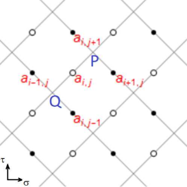
Figure 1: The string worldsheet (parametrized by $\tau$ and $\sigma$). Kink worldlines form a lattice and they collide in vertices ($P$, $Q$). The field $a_{ij}$ lives on the edges (black or white dots depending on edge orientation).

2.1 The discrete equation of motion

The motion of the string can be equivalently described using segmented strings [32, 33]. The classical theory is integrable which allows for the exact discretization of the equations. Solutions of the discrete equations correspond to string embeddings which consist of AdS₂ patches glued along null rays: the worldlines of kinks. Kink worldlines form a quad lattice on the worldsheet, see FIG. 1. Each diamond in the figure is a patch of AdS₂ with a constant normal vector which is defined as

$$N_{a}(z^{-},z^{+})\propto\epsilon_{abcd}Y^{b}\partial_{-}Y^{c}\partial_{+}Y^{d}\in{\mathbb{{R}}}^{2,2}\qquad\vec{N}^{2}=1$$

Indices are lowered and raised by $\eta=\textrm{diag}(-1,-1,+1,+1)$. The normal vector satisfies the same equation of motion as $\vec{Y}$ in (3), but with a plus sign [32, 33, 37, 35].

A discrete evolution equation for the normal vectors (or, equivalently, the kink collision points) has been found [32, 33] and can be used to build segmented string solutions. In [37] I showed that segmented strings in AdS₃ move according to the discrete equation of motion

$$\hskip-4.26773pt{1\over a_{ij}-a_{i,j+1}}+{1\over a_{ij}-a_{i,j-1}}={1\over a_{ij}-a_{i+1,j}}+{1\over a_{ij}-a_{i-1,j}}.$$ (4)

Here $i$ and $j$ are integer indices labeling lattice points on the string worldsheet. As illustrated in FIG. 1, kink worldlines pass through each of the lattice points (black and white dots). Kinks move with the speed of light both in target space and on the worldsheet. The dots are colored alternatingly, depending on which way the kink moves.

In FIG. 1, the variable $a_{ij}$ is expressed using the components of the difference vector $V\equiv P-Q\in{\mathbb{{R}}}^{2,2}$. If we define the $\mathfrak{a}:{\mathbb{{R}}}^{2,2}\to{\mathbb{{R}}}$ function as

$$\mathfrak{a}(\vec{X})\equiv{X_{-1}+X_{2}\over X_{0}+X_{1}}$$ (5)

then we simply have

$$a_{ij}=\mathfrak{a}(\vec{V})$$ (6)

and similarly the other $a$ variables are computed from their respective difference vectors. We will see shortly that they correspond to (advanced or retarded) boundary times.

Note that the equation of motion (4) is invariant under Möbius transformations,

$$a\to{c_{1}+c_{2}a\over c_{3}+c_{4}a}$$

which is due to the left $SL(2)$ factor in the AdS₃ isometry group $SO(2,2)=SL(2)\times SL(2)$. The $a$ field does not completely specify the string embedding: the right $SL(2)$ group only acts on the “right-handed” variables, which will be denoted by a tilde:

$$\tilde{a}_{ij}=\mathfrak{\tilde{a}}(\vec{V})\equiv{V_{-1}+V_{2}\over-V_{0}+V_{1}}\,.$$

The $\tilde{a}$ field satisfies the same equation as $a$ in (4).

What is the meaning of the $a$ field? The kink difference vectors (i.e. $V$ above) are null, therefore they correspond to points where the rays hit the boundary of AdS₃. In terms of the boundary Poincaré coordinates $t$ and $x$, the difference vector can be expressed as

$$\vec{V}\propto\left(\begin{array}[]{c}{-1+t^{2}-x^{2}}\\ 2t\\ 2x\\ {1+t^{2}-x^{2}}\end{array}\right).$$

from which we get

$$a = x^{-}$$

$$\tilde{a} = -x^{+}$$

where $x^{\pm}\equiv t\pm x$. If we now consider an embedding of AdS${}_{2}\subset$ AdS₃ with $x=0$ on the Poincaré patch, we see that the $a$ field tells us the retarded and advanced times at which kink null rays hit the boundary.

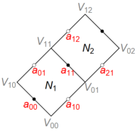
Figure 2: Two adjacent patches on the worldsheet.

3 Celestial fields

In this section we derive partial differential equations by taking an appropriate continuum limit of the discrete equation of motion (4).

3.1 Continuum limit

In general there are different ways to take a continuum limit of discrete equations. In the following we investigate the case where the $a$ variables over black dots and white dots (see FIG. 1) converge to two distinct fields. We will denote them by $b(z^{-},z^{+})$ and $w(z^{-},z^{+})$ and call them black and white celestial fields, respectively.

Let us consider two adjacent patches as in FIG. 2 and set

$$a_{11} = b(z^{-},z^{+})$$

$$a_{00} = b(z^{-},z^{+}-2\epsilon)$$

$$a_{10} = w(z^{-}-\epsilon,z^{+}-\epsilon)$$

$$a_{12} = w(z^{-}+\epsilon,z^{+}+\epsilon)$$

$$a_{01} = w(z^{-}+\epsilon,z^{+}-\epsilon)$$

$$a_{21} = w(z^{-}-\epsilon,z^{+}+\epsilon)$$ (7)

By taking the $\epsilon\to 0$ small lattice spacing limit, the discrete equation (4) becomes

$$\partial_{-}\partial_{+}w={2\partial_{-}w\,\partial_{+}w\over w-b}$$ (8)

and similarly for the black field

$$\partial_{-}\partial_{+}b={2\partial_{-}b\,\partial_{+}b\over b-w}.$$ (9)

In the continuum limit, the two fields can be computed via

$$b=\mathfrak{a}(\partial_{-}\vec{Y})\qquad\textrm{and}\qquad w=\mathfrak{a}(\partial_{+}\vec{Y})$$

where $\vec{Y}$ is the embedding function from (2). Note that the black and white fields transform as scalars under worldsheet conformal transformations.

3.2 Area densities $e^{\alpha}$ and $e^{\beta}$

Let us define the worldsheet area density $e^{\alpha}$ and the dual area density $e^{\beta}$ as follows:

$$\alpha(z^{-},z^{+})=\log\partial_{-}\vec{Y}\cdot\partial_{+}\vec{Y}$$

$$\beta(z^{-},z^{+})=\log\partial_{-}\vec{N}\cdot\partial_{+}\vec{N}$$

We can determine the area of an elementary patch of a segmented string [37]. For instance, the area of patch #1 in FIG. 1 is given by

$$A=\log\left({(a_{00}-a_{10})(a_{01}-a_{11})\over(a_{00}-a_{01})(a_{10}-a_{11})}\right)^{2}=e^{\alpha}(2\epsilon)^{2}$$

If we set the $a$ variables according to (7), then in the $\epsilon\to 0$ limit we get

$$e^{\alpha}=2{\partial_{+}b\,\partial_{-}w\over(b-w)^{2}}\qquad e^{\beta}=2{\partial_{-}b\,\partial_{+}w\over(b-w)^{2}}.$$ (10)

$\alpha$ is an important field, since as we will see it satisfies the generalized sinh-Gordon equation, and its exponential is the Nambu-Goto Lagrangian. Note that $e^{\alpha}$ is always non-negative whereas $e^{\beta}$ can be negative in certain regions on the worldsheet.

3.3 Target space vs. dual space

Let us consider two adjacent AdS₂ patches as in FIG. 2. If the normal vector $\vec{N}_{1}$ and the $a$ variables are known, then the vertices can be computed as follows. Let us define the antisymmetric matrix

$$M^{\mu\nu}_{(a,b)}={1\over a-b}\left(\begin{array}[]{cccc}0&-1-ab&1-ab&a+b\\ 1+ab&0&-a-b&1-ab\\ ab-1&a+b&0&-1-ab\\ -a-b&ab-1&1+ab&0\\ \end{array}\right)$$

where $a$ and $b$ are two parameters. Note that

$$M^{\mu\nu}_{(a,b)}=-M^{\mu\nu}_{(b,a)}\qquad\textrm{and}\qquad{M^{\mu}}_{\nu}{M^{\nu}}_{\kappa}=\delta^{\mu}_{\kappa}$$ (11)

where indices are raised by $\eta=\textrm{diag}(-1,-1,+1,+1)$.

Then the vertices are given by

$$(V_{00})^{\mu} = M^{\mu\nu}_{(a_{00},a_{10})}(N_{1})_{\nu}$$

$$(V_{01})^{\mu} = M^{\mu\nu}_{(a_{11},a_{10})}(N_{1})_{\nu}$$ (12)

and similarly for the other vertices: the two parameters of the $M$ matrix are the $a$ values sitting on the black and white dots near the vertex (see FIG. 1). Since $M^{\mu\nu}M_{\mu\kappa}=-\delta^{\nu}_{\kappa}$ and $N_{1}^{2}=1$, the vertices will be on the AdS hyperboloid, i.e. $V_{00}^{2}=V_{01}^{2}=-1$. Furthermore, since $M$ is antisymmetric, we will also have $V_{00}\cdot N_{1}=V_{01}\cdot N_{1}=0$, which means that they lie on the AdS₂ patch defined by $N_{1}$. Finally, it is easily shown that $\mathfrak{a}(V_{01}-V_{00})=a_{10}$. This means that the expressions for the vertices in (12) are indeed correct.

It can further be shown that

$$(N_{2})^{\mu}=M^{\mu\nu}_{(a_{11},a_{21})}(V_{01})_{\nu}\ .$$

Thus, if the $a$ variables are known, then the $M$ matrix can be used to switch between target space and dual space.

One can define an analogous antisymmetric matrix which does the same “reflection” operation, but this time using the tilde variables:

$$\widetilde{M}^{\mu\nu}_{(\tilde{a},\tilde{b})}={1\over\tilde{a}-\tilde{b}}\left(\begin{array}[]{cccc}0&-1-\tilde{a}\tilde{b}&-1+\tilde{a}\tilde{b}&-\tilde{a}-\tilde{b}\\ 1+\tilde{a}\tilde{b}&0&-\tilde{a}-\tilde{b}&1-\tilde{a}\tilde{b}\\ 1-\tilde{a}\tilde{b}&\tilde{a}+\tilde{b}&0&1+\tilde{a}\tilde{b}\\ \tilde{a}+\tilde{b}&\tilde{a}\tilde{b}-1&-1-\tilde{a}\tilde{b}&0\\ \end{array}\right).$$

Then we have

$$(V_{00})^{\mu}=\widetilde{M}^{\mu\nu}_{(\tilde{a}_{00},\tilde{a}_{10})}(N_{1})_{\nu}\ .$$ (13)

In the continuum limit, the $a$ variables converge to the $b$ and $w$ fields. Hence,

$$Y^{\mu}(z^{-},z^{+})=M^{\mu\nu}_{(b,w)}N_{\nu}(z^{-},z^{+})\ ,$$

$$N^{\mu}(z^{-},z^{+})=M^{\mu\nu}_{(b,w)}Y_{\nu}(z^{-},z^{+})\ .$$

3.4 The auxiliary $u$ and $v$ fields

Let us define the following quantities

$$u\equiv\partial_{-}N\cdot\partial_{-}Y=-N\cdot\partial_{-}\partial_{-}Y=-Y\cdot\partial_{-}\partial_{-}N$$

$$v\equiv-\partial_{+}N\cdot\partial_{+}Y=N\cdot\partial_{+}\partial_{+}Y=Y\cdot\partial_{+}\partial_{+}N$$

We need to find a properly discretized versions of these equations. If we set the $a_{ij}$ variables as in (7), and take

$$v\approx-(N_{2}-N_{1})\cdot(V_{01}-V_{00}){1\over(2\epsilon)^{2}}$$

then in the $\epsilon\to 0$ limit we get

$$v(z^{+})=2{\partial_{+}b\,\partial_{+}w\over(b-w)^{2}}$$

A similar calculation gives

$$u(z^{-})=2{\partial_{-}b\,\partial_{-}w\over(b-w)^{2}}\qquad$$

It is known that $\partial_{+}u=\partial_{-}v=0$. In fact, these two equations are equivalent to (8) and (9).

3.5 The generalized sinh-Gordon equation

By plugging in the expressions for $\alpha$, $u$, and $v$, it is easy to see that $\alpha$ satisfies the generalized sinh-Gordon equation

$$\partial_{-}\partial_{+}\alpha+e^{\alpha}-uve^{-\alpha}=0$$ (14)

This equation was first derived in [15] (see also [16]). Using

$$e^{\alpha+\beta}=uv$$

the sinh-Gordon equation can be re-written as

$$\partial_{-}\partial_{+}\alpha+e^{\alpha}-e^{\beta}=0$$

The dual field $\beta$ satisfies the same equation with $\alpha$ and $\beta$ exchanged:

$$\partial_{-}\partial_{+}\beta+e^{\beta}-e^{\alpha}=0$$

In a worldsheet region where $uv>0$ one can perform a conformal transformation and (locally) set $u(z^{-})=v(z^{+})=1$. We will call these balanced coordinates on the worldsheet. In these coordinates we have $\alpha=-\beta$. Note that these coordinates typically do not cover the entire worldsheet since $uv$ can change sign.

Finally, note that $\alpha$ can be expressed from $b$ and $u$ or $w$ and $v$:

$$e^{\alpha}={u}{\partial_{+}b\over\partial_{-}b}={v}{\partial_{-}w\over\partial_{+}w}$$ (15)

These formulas simplify even further in balanced coordinates when $u=v=1$.

3.6 Constraints

The discussion has so far focused on the continuum limit of the $a_{ij}$ field while neglecting the $\tilde{a}_{ij}$ variables and the corresponding $\tilde{b}$ and $\tilde{w}$ fields.

The $a$ and $\tilde{a}$ fields are not independent which can be seen as follows. Let us consider a single AdS₂ patch (see patch #1 in FIG 2). The patch is bounded by four kink worldlines. These are null vectors in ${\mathbb{{R}}}^{2,2}$ which can be constructed from the $a$ and $\tilde{a}$ variables. For instance,

$$\vec{p}^{(1)} \equiv \left(-1-a_{00}\tilde{a}_{00},\,a_{00}-\tilde{a}_{00},\,-a_{00}-\tilde{a}_{00},\,1-a_{00}\tilde{a}_{00}\right)\ \propto\ \vec{V}_{10}-\vec{V}_{00}$$

$$\vec{p}^{(2)} \equiv \left(-1-a_{10}\tilde{a}_{10},\,a_{10}-\tilde{a}_{10},\,-a_{10}-\tilde{a}_{10},\,1-a_{10}\tilde{a}_{10}\right)\ \propto\ \vec{V}_{01}-\vec{V}_{00}$$

$$\vec{p}^{(3)} \equiv \left(-1-a_{11}\tilde{a}_{11},\,a_{11}-\tilde{a}_{11},\,-a_{11}-\tilde{a}_{11},\,1-a_{11}\tilde{a}_{11}\right)\ \propto\ \vec{V}_{11}-\vec{V}_{01}$$

$$\vec{p}^{(4)} \equiv \left(-1-a_{01}\tilde{a}_{01},\,a_{01}-\tilde{a}_{01},\,-a_{01}-\tilde{a}_{01},\,1-a_{01}\tilde{a}_{01}\right)\ \propto\ \vec{V}_{11}-\vec{V}_{10}$$ (16)

It is easy to check that e.g. $\mathfrak{a}(\vec{p}^{(1)})=a_{00}$ and $\mathfrak{\tilde{a}}(\vec{p}^{(1)})=\tilde{a}_{00}$ and similarly for the other vectors. Since the sum of the four difference vectors (with appropriate signs) trivially vanishes, the determinant of the $4\times 4$ matrix constructed from the $p^{(i)}$ as row vectors must also vanish

$$\det\left(\begin{array}[]{cccc}p^{(1)}_{-1}&p^{(1)}_{0}&p^{(1)}_{1}&p^{(1)}_{2}\\ p^{(2)}_{-1}&p^{(2)}_{0}&p^{(2)}_{1}&p^{(2)}_{2}\\ p^{(3)}_{-1}&p^{(3)}_{0}&p^{(3)}_{1}&p^{(3)}_{2}\\ p^{(4)}_{-1}&p^{(4)}_{0}&p^{(4)}_{1}&p^{(4)}_{2}\end{array}\right)=0$$ (17)

This is one scalar constraint equation for the eight $a$ and $\tilde{a}$ variables around a patch. The remaining seven degrees of freedom completely specify the patch. This can be seen as follows. Let us fix the values of the $a$ and $\tilde{a}$ variables and keep $N_{1}$ arbitrary for the moment. Then four vertices $V_{00}$, $V_{10}$, $V_{01}$, and $V_{11}$ can be determined from (12) and four other vertices $\tilde{V}_{00}$, $\tilde{V}_{10}$, $\tilde{V}_{01}$, and $\tilde{V}_{11}$ using the analogous equation (13). Now if we set $V_{00}=\tilde{V}_{00}$ and $V_{10}=\tilde{V}_{10}$, then these equations completely determine the components of $N_{1}$. We get

$$\hskip-8.5359pt\vec{N}_{1}={\tiny{1\over\mathcal{C}}\left(\begin{array}[]{c}-a_{01}\tilde{a}_{10}(a_{00}(\tilde{a}_{01}-\tilde{a}_{00})+a_{10}\tilde{a}_{00}+1)+a_{10}(-\tilde{a}_{00}(a_{00}\tilde{a}_{01}+1)+a_{00}\tilde{a}_{01}\tilde{a}_{10}+\tilde{a}_{01})+a_{00}(\tilde{a}_{10}-\tilde{a}_{01})+a_{01}\tilde{a}_{00}(a_{10}\tilde{a}_{01}+1)\\ a_{00}(a_{01}(\tilde{a}_{01}-\tilde{a}_{00})+a_{10}\tilde{a}_{00}-a_{10}\tilde{a}_{10}-\tilde{a}_{00}\tilde{a}_{01}+\tilde{a}_{00}\tilde{a}_{10})+a_{01}(-a_{10}\tilde{a}_{01}+a_{10}\tilde{a}_{10}+\tilde{a}_{00}\tilde{a}_{01}-\tilde{a}_{01}\tilde{a}_{10})+a_{10}\tilde{a}_{10}(\tilde{a}_{01}-\tilde{a}_{00})\\ a_{00}(a_{01}(\tilde{a}_{00}-\tilde{a}_{01})-\tilde{a}_{00}(a_{10}+\tilde{a}_{01})+\tilde{a}_{10}(a_{10}+\tilde{a}_{00}))+a_{01}\tilde{a}_{01}(a_{10}+\tilde{a}_{00})-a_{01}\tilde{a}_{10}(a_{10}+\tilde{a}_{01})+a_{10}\tilde{a}_{10}(\tilde{a}_{01}-\tilde{a}_{00})\\ a_{01}(\tilde{a}_{00}(a_{00}\tilde{a}_{10}+a_{10}\tilde{a}_{01}-a_{10}\tilde{a}_{10}-1)-a_{00}\tilde{a}_{01}\tilde{a}_{10}+\tilde{a}_{10})+a_{10}(-a_{00}\tilde{a}_{00}\tilde{a}_{01}+a_{00}\tilde{a}_{01}\tilde{a}_{10}+\tilde{a}_{00}-\tilde{a}_{01})+a_{00}(\tilde{a}_{01}-\tilde{a}_{10})\end{array}\right)}$$ (18)

where the normalization factor is

$$\mathcal{C}^{2}\equiv 4(a_{01}-a_{00})(a_{00}-a_{10})(a_{01}-a_{10})(\tilde{a}_{00}-\tilde{a}_{01})(\tilde{a}_{00}-\tilde{a}_{10})(\tilde{a}_{01}-\tilde{a}_{10}).$$

Finally, for the other two vertices we get $V_{01}=\tilde{V}_{01}$ and $V_{11}=\tilde{V}_{11}$ if and only if the determinant (17) vanishes.

There is an analogous dual constraint for the difference vectors computed from four adjacent normal vectors. It is easy to see that in the continuum limit (17) and the dual constraint are tantamount to

$$\alpha={\tilde{\alpha}}\qquad\textrm{and}\qquad\beta={\tilde{\beta}}$$

where the $\tilde{\alpha}$ and $\tilde{\beta}$ are computed from the $\tilde{b}$ and $\tilde{w}$ fields:

$$e^{\tilde{\alpha}}=2{\partial_{+}\tilde{b}\,\partial_{-}\tilde{w}\over(\tilde{b}-\tilde{w})^{2}}\qquad e^{\tilde{\beta}}=2{\partial_{-}\tilde{b}\,\partial_{+}\tilde{w}\over(\tilde{b}-\tilde{w})^{2}}$$

Although it is not a separate constraint, one can derive an equation for $\tilde{u}$ and $\tilde{v}$ as well. The string equation of motion (3) says that $\vec{Y}\propto\partial_{-}\partial_{+}Y$. The normal vector satisfies an analogous equation of motion (with a plus sign). Thus we have

$$0=\vec{Y}\cdot\vec{N}\propto(\partial_{-}\partial_{+}Y)\cdot(\partial_{-}\partial_{+}N)$$ (19)

In order to express the right-hand side, similarly to (16), let us now take the following ansätze

$$\partial_{+}\vec{Y}=\lambda(z^{-},z^{+})\left(\begin{array}[]{c}-1-w\tilde{w}\\ w-\tilde{w}\\ -w-\tilde{w}\\ 1-w\tilde{w}\end{array}\right),\qquad\partial_{-}\vec{N}=\kappa(z^{-},z^{+})\left(\begin{array}[]{c}-1-w\tilde{w}\\ w-\tilde{w}\\ -w-\tilde{w}\\ 1-w\tilde{w}\end{array}\right)$$ (20)

with arbitrary proportionality factors $\lambda(z^{-},z^{+})$ and $\kappa(z^{-},z^{+})$. If we plug these expressions into (19), we get

$$2\lambda\kappa(\partial_{-}w\,\partial_{+}\tilde{w}+\partial_{+}w\,\partial_{-}\tilde{w})=0.$$

An analogous equation containing $b$ and $\tilde{b}$ can be derived if we start instead with a similar ansatz for $\partial_{-}\vec{Y}$ and $\partial_{+}\vec{N}$. Combining these equations with (15) we get the constraints

$$\tilde{u}=-u\qquad\tilde{v}=-v.$$

In addition to the above constraints, the area density must also be non-negative. This is ensured if the black and white fields satisfy

$$\partial_{+}b\,\partial_{-}w\geq 0.$$ (21)

3.7 String embedding

Given a solution of the sinh-Gordon equation, the string embedding can be computed by solving an auxiliary Dirac equation where $\alpha$ appears as a potential. If the $b$, $\tilde{b}$, $w$, $\tilde{w}$ fields are known, there is a simpler direct way to compute the embedding.

Similarly to (16), we can take the following ansatz for $\partial_{+}\vec{Y}$:

$$\partial_{+}\vec{Y}=\lambda(z^{-},z^{+})\left(\begin{array}[]{c}-1-w\tilde{w}\\ w-\tilde{w}\\ -w-\tilde{w}\\ 1-w\tilde{w}\end{array}\right).$$ (22)

The proportionality factor $\lambda(z^{-},z^{+})$ can be determined as follows. From the string equation of motion (3) we have

$$\vec{Y}=e^{-\alpha}\partial_{-}\partial_{+}\vec{Y}$$

and $\alpha$ can be expressed using $b$ and $w$ as in (10). If we plug in the $z$-derivative of (22), we can compute the norm of the position vector. We get

$$\vec{Y}^{2}=4e^{-2\alpha}\lambda^{2}\partial_{-}w\,\partial_{-}\tilde{w}$$

Note that terms containing partial derivatives of $\lambda$ have dropped out. Since the string must lie on the AdS₃ hyperboloid, we have $\vec{Y}^{2}=-1$, which determines $\lambda$ and therefore also the string embedding. However, the resulting expression is complicated and contains second derivatives of $b$ and $w$. A simpler formula can be obtained by taking the continuum limit of (18) and then converting it into a target space vector via (12). We get

$$\vec{Y}=\pm{1\over\mathcal{D}}\left(\begin{array}[]{c}(\tilde{w}-\tilde{b})(1+b\tilde{w})\partial_{-}w+(w-b)(1+\tilde{b}w)\partial_{-}\tilde{w}\\ (b-\tilde{w})(\tilde{b}-\tilde{w})\partial_{-}w+(b-w)(w-\tilde{b})\partial_{-}\tilde{w}\\ (\tilde{w}-\tilde{b})(b+\tilde{w})\partial_{-}w+(w-b)(\tilde{b}+w)\partial_{-}\tilde{w}\\ (\tilde{b}-\tilde{w})(1-b\tilde{w})\partial_{-}w+(b-w)(1-\tilde{b}w)\partial_{-}\tilde{w}\end{array}\right)$$

where the normalization factor is defined by

$$\mathcal{D}^{2}\equiv{-4(b-w)^{2}(\tilde{b}-\tilde{w})^{2}\partial_{-}w\,\partial_{-}\tilde{w}}.$$

3.8 The action

The Nambu-Goto action (after setting the prefactor to one)

$$S=\int\sqrt{-g}\,dz^{-}dz^{+}=\int e^{\alpha}dz^{-}dz^{+}$$

If we now plug in the expression (10) for $e^{\alpha}$, then we obtain the following action

$$S=2\int{\partial_{+}b\,\partial_{-}w\over(b-w)^{2}}dz^{-}dz^{+}$$

The Euler-Lagrange equations for $b$ and $w$ give the equations of motion (8) and (9). Note that only those solutions are allowed that satisfy (21).

The same equations of motion are obtained from the “dual” action

$$S^{\prime}=\int e^{\beta}dz^{-}dz^{+}=2\int{\partial_{+}w\,\partial_{-}b\over(b-w)^{2}}dz^{-}dz^{+}\,.$$

$S^{\prime}$ also appears in expressions for the regularized area of the worldsheet which equals the expectation value of the dual Wilson loop at strong coupling (see e.g. Appendix B of [44]).

3.9 Various limits

3.9.1 Flat space limit

In the flat space limit, the string worldsheet is mapped into an infinitesimal volume of AdS₃. Thus, the area density $e^{\alpha}$ vanishes and the generalized sinh-Gordon equation (14) degenerates into the Liouville equation

$$\partial_{-}\partial_{+}\alpha-uve^{-\alpha}=0$$

This equation can be explicitly solved in terms of two functions $f(z^{-})$ and $g(z^{+})$

$$e^{\alpha}={uv\over 2}{(f-g)^{2}\over f^{\prime}g^{\prime}}$$ (23)

This solution can be obtained using the black and white fields if we consider the limit

$$b(z^{-},z^{+})=b_{0}(z^{-})+\epsilon b_{1}(z^{-},z^{+})+\mathcal{O}(\epsilon^{2})\qquad w(z^{-},z^{+})=w_{0}(z^{+})+\epsilon w_{1}(z^{-},z^{+})+\mathcal{O}(\epsilon^{2})$$

as $\epsilon\to 0$. Here $b_{0}$ and $w_{0}$ are arbitrary functions, whereas $b_{1}$ and $w_{1}$ are determined from the equations of motion. Then, $\alpha$ can be determined from (10)

$$e^{\alpha}=uve^{-\beta}={uv\over 2}{(b_{0}-w_{0})^{2}\over b_{0}^{\prime}w_{0}^{\prime}}+\mathcal{O}(\epsilon^{2})$$

Comparing this with (23) gives $f=b_{0}$ and $g=w_{0}$.

3.9.2 AdS₂ limit

In the flat space limit one had $X(z^{-},z^{+})\approx X_{0}$ for a fixed $X_{0}\in{\mathbb{{R}}}^{2,2}$ vector in target space. One can consider a similar limit in the dual space of normal vectors, i.e. $N(z^{-},z^{+})\approx N_{0}$. In this case, the black and white fields become

$$b(z^{-},z^{+})\approx b_{0}(z^{+})\qquad\textrm{ and}\qquad w(z^{-},z^{+})\approx w_{0}(z^{-})$$

Note that the dependence of $b$ and $w$ on the worldsheet coordinates is swapped compared to the flat space limit.

3.9.3 Non-linear waves moving in one direction

One can consider non-linear waves moving in one direction on the string in AdS₃. In [45] Mikhailov gave an explicit expression for such solutions in terms of the position function of the string endpoint on the boundary. On the Poincaré patch the solution is

$$t(\tau,y) = \tau+{y\over\sqrt{1-x_{0}^{\prime}(\tau)^{2}}}$$

$$x(\tau,y) = x_{0}(\tau)+{yx_{0}^{\prime}(\tau)\over\sqrt{1-x_{0}^{\prime}(\tau)^{2}}}$$

$$y(\tau,y) = y$$ (24)

where $x_{0}(\tau)$ specifies the endpoint of the string in terms of the retarded time $\tau$. The induced metric is locally AdS₂ everywhere. The corresponding black and white fields can be computed with the result

$$b=b(z^{-},z^{+})\qquad w=w_{0}(z^{-})$$

We see that only $w$ has a special form. These solutions describe right-moving waves. For left-moving waves one has

$$b=b_{0}(z^{+})\qquad w=w(z^{-},z^{+})$$

Finally, one can consider a “dual” non-linear wave limit in which

$$b=b(z^{-},z^{+})\qquad w=w_{0}(z^{+})$$

and $b=b_{0}(z^{-})$, $w=w(z^{-},z^{+})$ for its left-moving counterpart.

4 Examples

The generalized sinh-Gordon equation in balanced coordinates gives the ordinary sinh-Gordon equation. This equation has singular soliton and antisoliton solutions, e.g.

$${\alpha}_{s,\bar{s}}=\pm\log\tanh^{2}{z^{-}-z^{+}\over\sqrt{2}}$$ (25)

There are explicit formulas for solutions containing solitons. The corresponding string embeddings have also been calculated, see [21, 25, 26, 28]. The string has a cusp whenever the $e^{\alpha}$ area density vanishes. This happens precisely at the location of a soliton.

In this section, we compute the black and white fields for a few examples.

4.1 Rotating string

The embedding is given by [20, 25]

$$\vec{Y}(\tau,\sigma)=\left(\begin{array}[]{c}\cosh\sigma\sin\tau\\ -\cosh\sigma\cos\tau\\ \sinh\sigma\cos\tau\\ \sinh\sigma\sin\tau\end{array}\right).$$

From this, we compute

$$b(z^{-},z^{+})=e^{z^{-}-z^{+}}\qquad w(z^{-},z^{+})=-e^{z^{-}-z^{+}}$$

$$\tilde{b}(z^{-},z^{+})={2\over 1-\tan{z^{-}+z^{+}\over 2}}-1\qquad\tilde{w}(z^{-},z^{+})=1-{2\over 1+\tan{z^{-}+z^{+}\over 2}}$$

and the auxiliary fields:

$$e^{\alpha}=e^{\tilde{\alpha}}=e^{\beta}=e^{\tilde{\beta}}=-u=\tilde{u}=-v=\tilde{v}={\frac{1}{2}}.$$

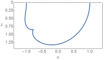
Figure 3: An example solution: a time-slice of the one-cusp solution on the Poincaré patch. The endpoints and the cusp move with the speed of light on the boundary and in the bulk, respectively.

4.2 String with one cusp

The embedding is given by [25]

$$\vec{Y}(\tau,\sigma)={1\over 2\sqrt{2}\cosh\sigma}\left(\begin{array}[]{c}2\tau\cos\tau-(2+\cosh 2\sigma)\sin\tau\\ 2\tau\sin\tau-(2+\cosh 2\sigma)\cos\tau\\ -2\tau\cos\tau+\sin\tau\cosh 2\sigma\\ -2\tau\sin\tau-\cos\tau\cosh 2\sigma\end{array}\right).$$

The black and white fields are

$$b(z^{-},z^{+})={1+z^{-}+z^{+}-\sinh(z^{-}-z^{+})\over 1-z^{-}-z^{+}+\sinh(z^{-}-z^{+})}\qquad w(z^{-},z^{+})={1+z^{-}+z^{+}+\sinh(z^{-}-z^{+})\over 1-z^{-}-z^{+}-\sinh(z^{-}-z^{+})}$$

$$\tilde{b}(z^{-},z^{+})={e^{z^{-}}+e^{z^{+}}\tan{z^{-}+z^{+}\over 2}\over e^{z^{+}}-e^{z^{-}}\tan{z^{-}+z^{+}\over 2}}\qquad\tilde{w}(z^{-},z^{+})={e^{z^{+}}+e^{z^{-}}\tan{z^{-}+z^{+}\over 2}\over e^{z^{-}}-e^{z^{+}}\tan{z^{-}+z^{+}\over 2}}$$

We further have

$$-u=\tilde{u}=-v=\tilde{v}={\frac{1}{2}},$$

and

$$e^{\alpha}=e^{\tilde{\alpha}}={1\over 4e^{\beta}}={1\over 4e^{\tilde{\beta}}}={\frac{1}{2}}\tanh^{2}{z^{-}-z^{+}\over 2}$$

which, in balanced coordinates, is nothing but the soliton solution (25).

4.3 String with two cusps

The embedding with two cusps is given via the following two complex functions [25]

$$Y_{-1}+iY_{0}=e^{-i\tau}{v\cosh T\cosh\sigma+\cosh X\cosh\sigma-\gamma^{-1}\sinh X\sinh\sigma+i\gamma^{-1}\sinh T\cosh\sigma\over\cosh T+v\cosh X}$$

$$Y_{1}+iY_{2}=e^{-i\tau}{v\cosh T\sinh\sigma+\cosh X\sinh\sigma-\gamma^{-1}\sinh X\cosh\sigma+i\gamma^{-1}\sinh T\sinh\sigma\over\cosh T+v\cosh X}$$

where $\gamma^{-1}=\sqrt{1-v^{2}}$ is the Lorentz factor, $T=2v\gamma\tau$, and $X=2\gamma\sigma$. Finally $v$ is the asymptotic speed of the two cusps on the worldsheet in the center-of-mass frame.

For the black and white fields we get

$$b(z^{-},z^{+})={\gamma^{-1}\sinh{z^{-}-z^{+}\over 2}\cosh\gamma(z^{-}-z^{+})-\cosh{z^{-}-z^{+}\over 2}\left[\sinh\gamma(z^{-}-z^{+})+\sinh v\gamma(z^{-}+z^{+})\right]\over\gamma^{-1}\cosh{z^{-}-z^{+}\over 2}\cosh\gamma(z^{-}-z^{+})-\sinh{z^{-}-z^{+}\over 2}\left[\sinh\gamma(z^{-}-z^{+})+\sinh v\gamma(z^{-}+z^{+})\right]}$$

$$w(z^{-},z^{+})={\gamma^{-1}\cosh{z^{-}-z^{+}\over 2}\cosh\gamma(z^{-}-z^{+})-\sinh{z^{-}-z^{+}\over 2}\left[\sinh\gamma(z^{-}-z^{+})-\sinh v\gamma(z^{-}+z^{+})\right]\over\gamma^{-1}\sinh{z^{-}-z^{+}\over 2}\cosh\gamma(z^{-}-z^{+})-\cosh{z^{-}-z^{+}\over 2}\left[\sinh\gamma(z^{-}-z^{+})-\sinh v\gamma(z^{-}+z^{+})\right]}$$

The expressions for $\tilde{b}$ and $\tilde{w}$ are too large to be presented here. A calculation yields

$$e^{\alpha}={1\over 4e^{\beta}}={\frac{1}{2}}\left(1-{2\over 1+v{\cosh\gamma(z^{-}-z^{+})\over\cosh v\gamma(z^{-}+z^{+})}}\right)^{2}$$

and

$$u=v=-{\frac{1}{2}}.$$

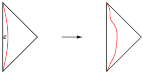
Figure 4: Explicitly broken conformal symmetry: AdS₂ is cut off a distance $\epsilon$ away from the boundary (red line). Under a conformal transformation this UV boundary moves around and therefore the value of the action changes.

5 The Schwarzian action

The Sachdev-Ye-Kitaev model [46, 47], the 2d gravity model of Jackiw and Teitelboim [48, 49] and certain other gravity models [50] can be described at low energies in terms of a degree of freedom which is a function of one variable and describes reparametrizations of (imaginary) time. The aim of this section is to derive this effective action for a string worldsheet which is an AdS₂ slice of the AdS₃ target space.

Let us therefore consider a string with a constant normal vector. The induced metric on the worldsheet is AdS₂. Small perturbations around the static embedding behave like a matter field with conformal dimension $\Delta=1$. “Conformal symmetry” on the boundary is the reparametrization symmetry

$$b\to f(b)\qquad\textrm{and}\qquad w\to f(w)$$ (26)

This symmetry is spontaneously broken down to $SL(2)$, i.e. simultaneous Möbius transformations

$$b\to{c_{1}+c_{2}b\over c_{3}+c_{4}b}\qquad\textrm{and}\qquad w\to{c_{1}+c_{2}w\over c_{3}+c_{4}w}$$

which still preserve the form of the equations of motion (8) and (9). There is an analogous symmetry breaking associated to the right-handed fields $\tilde{b}$ and $\tilde{w}$.

One can introduce an explicit conformal symmetry breaking by cutting out a piece of AdS₂ in the UV region as in FIG. 4. Under a conformal transformation (26) this boundary changes and thus the value of the action also changes. Let us use worldsheet coordinates such that $b=z^{+}$ and $w=z^{-}$. Then the change in the action can be computed using (10),

$$\Delta S=\int dz^{-}dz^{+}\left(e^{\alpha[f(b),f(w)]}-e^{\alpha[b,w]}\right)=2\int dz^{-}dz^{+}\left[{f^{\prime}(z^{-})f^{\prime}(z^{+})\over(f(z^{-})-f(z^{+}))^{2}}-{1\over(z^{-}-z^{+})^{2}}\right]$$

In FIG. 4, the original AdS₂ boundary is the vertical black line. On the boundary, retarded and advanced times are equal, i.e. $b=w$. In our gauge this is at $z^{-}=z^{+}$. Let us now introduce the UV cutoff (red line in the figure) at

$$z^{-}=z^{-}_{\epsilon}\equiv z^{+}+\epsilon\varphi(z^{+})$$

Here we have included a varying coupling $\varphi(z^{+})$. After performing the $z^{-}$ integral between $-\infty$ and the UV cutoff $z_{\epsilon}^{-}$, we get

$$\Delta S=2\int dz^{+}\left[{f^{\prime}(z^{+})\over f(z^{+})-f(z_{\epsilon}^{-})}-{1\over z^{+}-z_{\epsilon}^{-}}\right]$$

For small $\epsilon$, the integrand can be Taylor expanded. Assuming $f^{\prime}(+\infty)=f^{\prime}(-\infty)$ we get

$$\Delta S\approx{2\epsilon\over 3}\int dz^{+}\,\varphi(z^{+})\left[{f^{\prime\prime\prime}(z^{+})\over f^{\prime}(z^{+})}-{3\over 2}{f^{\prime\prime}(z^{+})^{2}\over f^{\prime}(z^{+})^{2}}\right]$$

This is the Schwarzian action [47, 52, 53, 51, 54]. Related expressions for the renormalized string area in the Euclidean case were obtained in [44] (see also [55, 56, 57, 58]). In the Lorentzian case the above Schwarzian action for the string was computed in [59].

5.1 An exact Schwarzian on the worldsheet

The Euler-Lagrange equations for the Schwarzian action produce a fourth order differential equation. Note that if $w$ is expressed using (9) as

$$w=b-{2\partial_{-}b\,\partial_{+}b\over\partial_{-}\partial_{+}b}$$

then (8) will give a fourth order equation for $b$.

Let us compute the change in the action if $w$ is kept on-shell and $b$ is transformed $b\to f(b)$. We obtain

$$\Delta S=\int dz^{-}dz^{+}\left(e^{\alpha[f(b)]}-e^{\alpha[b]}\right)={\frac{1}{2}}\int dz^{-}dz^{+}\left[{f^{\prime\prime\prime}(b)\over f^{\prime}(b)}-{3\over 2}{f^{\prime\prime}(b)^{2}\over f^{\prime}(b)^{2}}\right]\partial_{-}b\,\partial_{+}b$$

It is interesting to see the appearance of the Schwarzian again. In this case it is integrated over the two-dimensional worldsheet. Note, however, that this expression for the action is exact and it does not require the embedding to be special (e.g. close to an AdS₂ slice).

6 Discussion

In this paper we have considered a Nambu-Goto string in AdS₃ spacetime. We have mainly used the embedding into ambient space: $Y(z^{-},z^{+})\in$ AdS₃ $\subset{\mathbb{{R}}}^{2,2}$ (here $z^{\pm}$ are null coordinates on the Lorentzian worldsheet). By taking a continuum limit of the discrete equation of motion of segmented strings, we have obtained differential equations for a smooth string in terms of two fields

$$b(z^{-},z^{+})\equiv\mathfrak{a}(\partial_{-}Y)\qquad w(z^{-},z^{+})\equiv\mathfrak{a}(\partial_{+}Y)$$

where $\mathfrak{a}(X)={X_{-1}+X_{2}\over X_{0}+X_{1}}$. Our main results are the following equations of motion

$$\partial_{-}\partial_{+}w=2{\partial_{-}w\,\partial_{+}w\over w-b},\qquad\partial_{-}\partial_{+}b=2{\partial_{-}b\,\partial_{+}b\over b-w}.$$

We define the following auxiliary fields: the area density $e^{\alpha}$, the area density in the space of normal vectors $e^{\beta}$, and the $u$ and $v$ fields. They are given by

$$e^{\alpha(z^{-},z^{+})}=2{\partial_{+}b\,\partial_{-}w\over(b-w)^{2}},\qquad e^{\beta(z^{-},z^{+})}=2{\partial_{-}b\,\partial_{+}w\over(b-w)^{2}},$$

$$u(z^{-})=2{\partial_{-}b\,\partial_{-}w\over(b-w)^{2}},\qquad v(z^{+})=2{\partial_{+}b\,\partial_{+}w\over(b-w)^{2}}.$$

Using the equations of motion it is easy to see that the auxiliary fields satisfy the generalized sinh-Gordon equations [15]

$$\partial_{-}\partial_{+}\alpha+e^{\alpha}-uve^{-\alpha}=0,$$

$$\partial_{-}\partial_{+}\beta+e^{\beta}-uve^{-\beta}=0.$$

There are analogous equations for the right-handed fields that we denote with a tilde. Instead of $\mathfrak{a}$, these are defined using $\mathfrak{\tilde{a}}(X)={X_{-1}+X_{2}\over-X_{0}+X_{1}}$. The right-handed fields are not independent, because the constraints

$$\alpha={\tilde{\alpha}},\qquad\beta={\tilde{\beta}},\qquad u=-\tilde{u},\qquad v=-\tilde{v}$$

must be satisfied by the $b$, $w$, $\tilde{b}$, $\tilde{w}$ fields. In particular, $\alpha={\tilde{\alpha}}$ means that the right-handed variables must give the same induced metric on the worldsheet as the left-handed ones.

A potential application of the celestial variables developed in [37, 38] and in the current paper is an alternative calculation of the spectral curve. Preliminary results show that in certain cases it is possible to write down explicit expressions for the quasimomenta without the use of transcendental functions [61].

The theory on the string worldsheet shares many features with theories of quantum gravity [14]. The $b$ and $w$ fields are in a certain sense holographic: they describe the string embedding using coordinates at null infinity. One might hope that the string worldsheet has a holographic description and that the celestial fields play a role in this.

In the flat space (or the dual near-AdS₂) limit the generalized sinh-Gordon equation degenerates and becomes the Liouville equation. This can be solved explicitly in terms of two arbitrary function (see section 3.9.1). As one can see from the expression for $e^{\alpha}$ in (10), the celestial fields provide a generalization of the Liouville solution which is applicable to the sinh-Gordon equation. Although the description contains two fields, there is only one physical degree of freedom: the transverse position of the string in the AdS₃ target space.

The string embedding can be computed from a sinh-Gordon solution if one solves an associated Dirac scattering problem, see e.g. [62]. In the Appendix we discuss how the black and white celestial fields can be expressed as ratios of the spinor components of the solution.

In this paper we have used Poincaré coordinates. In global AdS coordinates the form of the equation change. This can be seen by replacing $b\to\tan b$ and $w\to\tan w$. The new celestial fields now correspond to retarded and advanced boundary times in global AdS coordinates at which null rays emanating from the string reach the boundary. Due to the nature of the immersion of AdS₃ into ${\mathbb{{R}}}^{2,2}$ in (1) the time coordinates are periodic, therefore $b$ and $w$ are coordinates on a torus. By plugging in the tangent functions into (8) and (9) it is easy to see that they satisfy the equations

$$\partial_{-}\partial_{+}w=2{\partial_{-}w\,\partial_{+}w\over\tan(w-b)},\qquad\partial_{-}\partial_{+}b=2{\partial_{-}b\,\partial_{+}b\over\tan(b-w)}.$$

Similar equations are also expected to be valid when the target space is de Sitter spacetime [15, 35]. The string worldsheet can also be coupled to a background two-form whose field strength is the volume form of AdS₃ (i.e. the coupling does not destroy any of the continuous symmetries of the system [36]). Independently of the value of the coupling, the discrete equation of motion in (4) remains the same [38] and thus the $b$ and $w$ fields will satisfy the same equations of motion. Finally, a higher-dimensional generalization may be possible since the spinor-helicity formalism has been extended to higher dimensions (see e.g [63]). In AdS₃ left- and right-handed celestial fields ($b,w$ and $\tilde{b},\tilde{w}$, respectively) decouple. Thus one can concentrate on either pair without having to deal with constraints between them. In general dimensions one does not expect such a decoupling. This makes AdS₃ special.

Acknowledgments

I thank Martin Kruczenski, Douglas Stanford, and the referee for valuable comments on the manuscript. The author is supported by the STFC Ernest Rutherford grant ST/P004334/1.

Appendix

The string embedding can be computed from a sinh-Gordon solution if one solves an associated scattering problem of a spinor field. In this Appendix we will discuss how the black and white celestial fields can be expressed as ratios of the spinor components of the solution. The $SL(2)$ Lax matrices are [62]

$$B^{-}_{L}=\begin{pmatrix}{1\over 4}\partial_{-}\alpha&{1\over\sqrt{2}}{e^{{\alpha\over 2}}}\cr{u\over\sqrt{2}}{e^{-{\alpha\over 2}}}&-{1\over 4}\partial_{-}\alpha\end{pmatrix} B^{+}_{L}=\begin{pmatrix}-{1\over 4}\partial_{+}\alpha&-{v\over\sqrt{2}}{e^{-{\alpha\over 2}}}\cr-{1\over\sqrt{2}}e^{{\alpha\over 2}}&{1\over 4}\partial_{+}\alpha\end{pmatrix}$$

$$B^{-}_{R}=\begin{pmatrix}-{1\over 4}\partial_{-}\alpha&{-{u\over\sqrt{2}}e^{-{\alpha\over 2}}}\cr{1\over\sqrt{2}}{e^{{\alpha\over 2}}}&{1\over 4}\partial_{-}\alpha\end{pmatrix} B^{+}_{R}=\begin{pmatrix}{1\over 4}\partial_{+}\alpha&-{1\over\sqrt{2}}{e^{{\alpha\over 2}}}\cr{v\over\sqrt{2}}{e^{-{\alpha\over 2}}}&-{1\over 4}\partial_{+}\alpha\end{pmatrix}\,.$$

The flatness conditions

$$\partial_{-}B^{+}_{L}-\partial_{+}B^{-}_{L}+[B^{-}_{L},B^{+}_{L}] = 0\,,$$

$$\partial_{-}B^{+}_{R}-\partial_{+}B^{-}_{R}+[B^{-}_{R},B^{+}_{R}] = 0$$

are equivalent to the sinh-Gordon equation. Let us now consider the left and right linear systems

$$\partial_{-}\psi^{L}_{\alpha}+(B^{-}_{L})_{\alpha}^{~{}\beta}\psi^{L}_{\beta}=0\,, \partial_{+}\psi^{L}_{\alpha}+(B^{+}_{L})_{\alpha}^{~{}\beta}\psi^{L}_{\beta}=0\,,$$

$$\partial_{-}\psi^{R}_{\dot{\alpha}}+(B^{-}_{R})_{\dot{\alpha}}^{~{}\dot{\beta}}\psi^{R}_{\dot{\beta}}=0\,, \partial_{+}\psi^{R}_{\dot{\alpha}}+(B^{+}_{R})_{\dot{\alpha}}^{~{}\dot{\beta}}\psi^{R}_{\dot{\beta}}=0\,.\quad$$ (27)

where $\psi^{L}_{\alpha}$ and $\psi^{R}_{\dot{\alpha}}$ are two-component spinors ($\alpha,\dot{\alpha}\in\{0,1\}$). Each of these systems have two linearly independent solutions, denoted by $\psi^{L}_{\alpha a}$ and $\psi^{R}_{\dot{\alpha}\dot{a}}$ (here $a,\dot{a}\in\{0,1\}$ label the independent solutions). We will normalize them so that

$$\epsilon^{\beta\alpha}\psi^{L}_{\alpha a}\psi^{L}_{\beta b}=\epsilon_{ab},~{}~{}~{}~{}~{}\epsilon^{\dot{\beta}\dot{\alpha}}\psi^{R}_{\dot{\alpha}\dot{a}}\psi^{R}_{\dot{\beta}\dot{b}}=\epsilon_{\dot{a}\dot{b}}$$ (28)

where $\epsilon$ is the $2\times 2$ Levi-Civita tensor. Using the spinor solutions, one can compute the matrix [62]

$$W={\frac{1}{2}}\begin{pmatrix}Y+N&{e^{-{\alpha\over 2}}\partial_{+}Y}\cr{e^{-{\alpha\over 2}}}\partial_{-}Y&Y-N\end{pmatrix}\,,$$

where $Y(z^{-},z^{+})$ is the embedding function, $N(z^{-},z^{+})$ is the normal vector function. Let $\alpha,\dot{\alpha}$ denote the indices of the $2\times 2$ matrix, and use the equivalence of $SO(2,2)$ and $SL(2)\times SL(2)$ to decompose spacetime indices into spinor indices $a,\dot{a}$. The result is a quantity with four spinor indices $W=W_{\alpha\dot{\alpha},a\dot{a}}$. The trace computes the string embedding which is given by

$$Y_{a\dot{a}}\equiv\begin{pmatrix}Y_{-1}+Y_{2}&Y_{1}-Y_{0}\cr Y_{1}+Y_{0}&Y_{-1}-Y_{2}\end{pmatrix}_{a,\dot{a}}=\psi^{L}_{\alpha,a}M_{1}^{\alpha\dot{\beta}}\psi^{R}_{\dot{\beta},\dot{a}}$$ (29)

where $M_{1}=\textrm{diag}(1,1)$. Similarly, one can compute $e^{-{\alpha\over 2}}\partial_{\pm}Y$ by replacing $M_{1}$ with another matrix. By taking ratios one can obtain the $b$ and $w$ fields,

$$b(z^{-},z^{+})={(\partial_{-}Y)_{-1}+(\partial_{-}Y)_{2}\over(\partial_{-}Y)_{1}+(\partial_{-}Y)_{0}}={\psi^{L}_{10}\psi^{R}_{\dot{0}\dot{0}}\over\psi^{L}_{11}\psi^{R}_{\dot{0}\dot{0}}}={\psi^{L}_{10}\over\psi^{L}_{11}}\,.$$

Similarly, we have

$$w(z^{-},z^{+})={(\partial_{+}Y)_{-1}+(\partial_{+}Y)_{2}\over(\partial_{+}Y)_{0}+(\partial_{+}Y)_{1}}={\psi^{L}_{00}\over\psi^{L}_{01}}\,.$$

Note that the right spinors have dropped out from the final expressions.

One can also compute the ‘right-handed’ celestial fields

$$\tilde{b}(z^{-},z^{+})={(\partial_{-}Y)_{-1}+(\partial_{-}Y)_{2}\over(\partial_{-}Y)_{1}-(\partial_{-}Y)_{0}}={\psi^{L}_{10}\psi^{R}_{\dot{0}\dot{0}}\over\psi^{L}_{10}\psi^{R}_{\dot{0}\dot{1}}}={\psi^{R}_{\dot{0}\dot{0}}\over\psi^{R}_{\dot{0}\dot{1}}}\,,$$

and

$$\tilde{w}(z^{-},z^{+})={(\partial_{+}Y)_{-1}+(\partial_{+}Y)_{2}\over(\partial_{+}Y)_{1}-(\partial_{+}Y)_{0}}={\psi^{R}_{\dot{1}\dot{0}}\over\psi^{R}_{\dot{1}\dot{1}}}\,.$$

These formulas relate the celestial fields to the solutions of the linear problem.

References

• [1] T. Ishii and K. Murata, Turbulent strings in AdS/CFT, JHEP 06 (2015) 086 [1504.02190].
• [2] D. Vegh, Pair-production of cusps on a string in AdS3, 1802.04306.
• [3] J. M. Maldacena, The large N limit of superconformal field theories and supergravity, Adv. Theor. Math. Phys. 2 (1998) 231–252.
• [4] S. S. Gubser, I. R. Klebanov and A. M. Polyakov, Gauge theory correlators from non-critical string theory, Phys. Lett. B428 (1998) 105–114 [hep-th/9802109].
• [5] E. Witten, Anti-de Sitter space and holography, Adv. Theor. Math. Phys. 2 (1998) 253–291.
• [6] C. P. Herzog, A. Karch, P. Kovtun, C. Kozcaz and L. G. Yaffe, Energy loss of a heavy quark moving through N=4 supersymmetric Yang-Mills plasma, JHEP 07 (2006) 013 [hep-th/0605158].
• [7] H. Liu, K. Rajagopal and U. A. Wiedemann, Calculating the jet quenching parameter from AdS/CFT, Phys. Rev. Lett. 97 (2006) 182301 [hep-ph/0605178].
• [8] S. S. Gubser, Drag force in AdS/CFT, Phys. Rev. D74 (2006) 126005 [hep-th/0605182].
• [9] J. Maldacena, S. H. Shenker and D. Stanford, A bound on chaos, JHEP 08 (2016) 106 [1503.01409].
• [10] S. H. Shenker and D. Stanford, Black holes and the butterfly effect, JHEP 03 (2014) 067 [1306.0622].
• [11] S. H. Shenker and D. Stanford, Multiple Shocks, JHEP 12 (2014) 046 [1312.3296].
• [12] K. Murata, Fast scrambling in holographic Einstein-Podolsky-Rosen pair, JHEP 11 (2017) 049 [1708.09493].
• [13] J. de Boer, E. Llabres, J. F. Pedraza and D. Vegh, Chaotic strings in AdS/CFT, Phys. Rev. Lett. 120 (2018), no. 20 201604 [1709.01052].
• [14] S. Dubovsky, R. Flauger and V. Gorbenko, Solving the Simplest Theory of Quantum Gravity, JHEP 09 (2012) 133 [1205.6805].
• [15] K. Pohlmeyer, Integrable Hamiltonian Systems and Interactions Through Quadratic Constraints, Commun. Math. Phys. 46 (1976) 207–221.
• [16] H. J. De Vega and N. G. Sanchez, Exact integrability of strings in D-Dimensional De Sitter space-time, Phys. Rev. D47 (1993) 3394–3405.
• [17] I. Bena, J. Polchinski and R. Roiban, Hidden symmetries of the AdS(5) x S**5 superstring, Phys. Rev. D69 (2004) 046002 [hep-th/0305116].
• [18] N. Beisert et. al., Review of AdS/CFT Integrability: An Overview, Lett. Math. Phys. 99 (2012) 3–32 [1012.3982].
• [19] A. A. Tseytlin, Review of AdS/CFT Integrability, Chapter II.1: Classical AdS5xS5 string solutions, Lett. Math. Phys. 99 (2012) 103–125 [1012.3986].
• [20] S. S. Gubser, I. R. Klebanov and A. M. Polyakov, A Semiclassical limit of the gauge / string correspondence, Nucl. Phys. B636 (2002) 99–114 [hep-th/0204051].
• [21] M. Kruczenski, Spiky strings and single trace operators in gauge theories, JHEP 08 (2005) 014 [hep-th/0410226].
• [22] C. Kalousios, M. Spradlin and A. Volovich, Dressing the giant magnon II, JHEP 03 (2007) 020 [hep-th/0611033].
• [23] L. F. Alday and J. M. Maldacena, Gluon scattering amplitudes at strong coupling, JHEP 06 (2007) 064 [0705.0303].
• [24] M. Grigoriev and A. A. Tseytlin, Pohlmeyer reduction of AdS(5) x S**5 superstring sigma model, Nucl. Phys. B800 (2008) 450–501 [0711.0155].
• [25] A. Jevicki, K. Jin, C. Kalousios and A. Volovich, Generating AdS String Solutions, JHEP 0803 (2008) 032 [0712.1193].
• [26] A. Jevicki and K. Jin, Solitons and AdS String Solutions, Int. J. Mod. Phys. A23 (2008) 2289–2298 [0804.0412].
• [27] N. Dorey and M. Losi, Spiky Strings and Spin Chains, 0812.1704.
• [28] A. Jevicki and K. Jin, Moduli Dynamics of AdS(3) Strings, JHEP 06 (2009) 064 [0903.3389].
• [29] N. Dorey and M. Losi, Giant Holes, J. Phys. A43 (2010) 285402 [1001.4750].
• [30] N. Dorey and M. Losi, Spiky Strings and Giant Holes, JHEP 12 (2010) 014 [1008.5096].
• [31] A. Irrgang and M. Kruczenski, Rotating Wilson loops and open strings in AdS3, J.Phys. A46 (2013) 075401 [1210.2298].
• [32] D. Vegh, The broken string in anti-de Sitter space, JHEP 02 (2018) 045 [1508.06637].
• [33] N. Callebaut, S. S. Gubser, A. Samberg and C. Toldo, Segmented strings in AdS3, JHEP 11 (2015) 110 [1508.07311].
• [34] D. Vegh, Colliding waves on a string in AdS3, 1509.05033.
• [35] S. S. Gubser, Evolution of segmented strings, Phys. Rev. D94 (2016), no. 10 106007 [1601.08209].
• [36] S. S. Gubser, S. Parikh and P. Witaszczyk, Segmented strings and the McMillan map, JHEP 07 (2016) 122 [1602.00679].
• [37] D. Vegh, Segmented strings from a different angle, 1601.07571.
• [38] D. Vegh, Segmented strings coupled to a B-field, JHEP 04 (2018) 088 [1603.04504].
• [39] X. Artru, Classical String Phenomenology. 1. How Strings Work, Phys. Rept. 97 (1983) 147.
• [40] B. Andersson, G. Gustafson, G. Ingelman and T. Sjostrand, Parton Fragmentation and String Dynamics, Phys. Rept. 97 (1983) 31–145.
• [41] Y. B. Suris, The Problem of Integrable Discretization: Hamiltonian Approach. Birkhäuser Verlag, Basel, 2003.
• [42] S. Pasterski, S.-H. Shao and A. Strominger, Flat Space Amplitudes and Conformal Symmetry of the Celestial Sphere, Phys. Rev. D 96 (2017), no. 6 065026 [1701.00049].
• [43] A. Atanasov, A. Ball, W. Melton, A.-M. Raclariu and A. Strominger, $(2,2)$ Scattering and the Celestial Torus, 2101.09591.
• [44] M. Kruczenski, Wilson loops and minimal area surfaces in hyperbolic space, JHEP 11 (2014) 065 [1406.4945].
• [45] A. Mikhailov, Nonlinear waves in AdS / CFT correspondence, hep-th/0305196.
• [46] S. Sachdev and J. Ye, Gapless spin-fluid ground state in a random quantum heisenberg magnet, Phys. Rev. Lett. 70 (May, 1993) 3339–3342.
• [47] A. Kitaev, A Simple Model of Quantum Holography, Talks at KITP, April 7, 2015 and May 27, 2015, http://online.kitp.ucsb.edu/online/entangled15/kitaev , .
• [48] R. Jackiw, Lower dimensional gravity, Nuclear Physics B 252 (1985) 343 – 356.
• [49] C. Teitelboim, Gravitation and hamiltonian structure in two spacetime dimensions, Physics Letters B 126 (1983), no. 1 41 – 45.
• [50] A. Almheiri and J. Polchinski, Models of AdS2 backreaction and holography, JHEP 11 (2015) 014 [1402.6334].
• [51] J. Maldacena, D. Stanford and Z. Yang, Conformal symmetry and its breaking in two dimensional Nearly Anti-de-Sitter space, PTEP 2016 (2016), no. 12 12C104 [1606.01857].
• [52] J. Maldacena and D. Stanford, Remarks on the Sachdev-Ye-Kitaev model, Phys. Rev. D94 (2016), no. 10 106002 [1604.07818].
• [53] K. Jensen, Chaos in AdS2 Holography, Phys. Rev. Lett. 117 (2016), no. 11 111601 [1605.06098].
• [54] J. Engelsoy, T. G. Mertens and H. Verlinde, An investigation of AdS2 backreaction and holography, JHEP 07 (2016) 139 [1606.03438].
• [55] A. Irrgang and M. Kruczenski, Euclidean Wilson loops and minimal area surfaces in lorentzian AdS3, JHEP 12 (2015) 083 [1507.02787].
• [56] A. Dekel, Wilson Loops and Minimal Surfaces Beyond the Wavy Approximation, JHEP 03 (2015) 085 [1501.04202].
• [57] C. Huang, Y. He and M. Kruczenski, Minimal area surfaces dual to Wilson loops and the Mathieu equation, JHEP 08 (2016) 088 [1604.00078].
• [58] Y. He, C. Huang and M. Kruczenski, Minimal area surfaces in AdS(n+1) and Wilson loops, JHEP 02 (2018) 027 [1712.06269].
• [59] A. Banerjee, A. Kundu and R. R. Poojary, Strings, Branes, Schwarzian Action and Maximal Chaos, 1809.02090.
• [60] B. R. Greene, A. D. Shapere, C. Vafa and S.-T. Yau, Stringy cosmic strings and noncompact Calabi-Yau manifolds, Nucl. Phys. B337 (1990) 1.
• [61] D. Vegh, “Work in progress.”
• [62] L. F. Alday and J. Maldacena, Null polygonal Wilson loops and minimal surfaces in Anti-de-Sitter space, JHEP 0911 (2009) 082 [0904.0663].
• [63] C. Cheung and D. O’Connell, Amplitudes and Spinor-Helicity in Six Dimensions, JHEP 07 (2009) 075 [0902.0981].