Reducing Service Deployment Cost
Through VNF Sharing

Abstract

Thanks to its computational and forwarding capabilities, the mobile network infrastructure can support several third-party (“vertical”) services, each composed of a graph of virtual (network) functions (VNFs). Importantly, one or more VNFs are often common to multiple services, thus the services deployment cost could be reduced by letting the services share the same VNF instance instead of devoting a separate instance to each service. By doing that, however, it is critical that the target KPI (key performance indicators) of all services are met. To this end, we study the VNF sharing problem and make decisions on (i) when sharing VNFs among multiple services is possible, (ii) how to adapt the virtual machines running the shared VNFs to the combined load of the assigned services, and (iii) how to prioritize the services traffic within shared VNFs. All decisions aim to minimize the cost for the mobile operator, subject to requirements on end-to-end service performance, e.g., total delay. Notably, we show that the aforementioned priorities should be managed dynamically and vary across VNFs. We then propose the FlexShare algorithm to provide near-optimal VNF-sharing and priority assignment decisions in polynomial time. We prove that FlexShare is within a constant factor from the optimum and, using real-world VNF graphs, we show that it consistently outperforms baseline solutions.

I Introduction

Emerging mobile networks do not only forward data, but they can also process the data: based on the software-defined networking (SDN) and the network function virtualization (NFV) paradigms, they run virtual (network) functions (VNFs) and perform network-related (e.g., firewalls) or service-specific (e.g., video transcoding) tasks. Such processing at the edge of the network infrastructure allows for lower latency, higher efficiency, and lower costs compared to current cloud-based architecture. These new capabilities of network systems bring forth a new relationship between mobile network operators (MNOs) and third-party companies (“verticals”) providing the services. On the one hand, verticals make business agreements with MNOs, specifying (i) the service they wish to run, defined by a VNF graph, i.e., the set of VNFs composing the service, properly connected to each other; (ii) the end-to-end target key performance indicators (KPIs), e.g., throughput, delay, or reliability for each service. On the other hand, MNOs seek to maintain the target KPIs of the deployed services while minimizing their deployment cost. Inefficiently-used infrastructure can indeed result into significant costs for the MNO, thus jeopardizing its revenue: as an example, [1] reports that idle servers consume 60% of their peak power.

To efficiently support multiple services, the network slicing paradigm for backhaul infrastructure has been introduced [2]. Under this paradigm, the mobile operator’s backhaul infrastructure, e.g., routers and servers, supports services from different verticals, while guaranteeing isolation and honoring the target KPIs of each service. Network slicing also supports composed services (i.e., services whose VNF graphs include sub-graphs, each corresponding to a child service [3]), thus enabling the corresponding slices to include common sub-slices [4, 5]. A typical example of a child service is the cellular Evolved Packet Core (EPC) [3], which is a common component of the mobile services required by the verticals.

Upon creating a slice, MNOs must (i) assign it the necessary resources (e.g., virtual machines and virtual links connecting them), and (ii) decide which VNFs to run at each host. The latter problem, known as the VNF placement problem, is often formulated as a cost minimization problem subject to the target KPIs. Importantly, significant cost savings can be achieved by sharing individual VNFs or sub-slices among services, whenever possible. The vast majority of VNF placement studies [6, 7, 8, 9] consider scenarios where all placement decisions are made by a centralized entity, often the NFV Orchestrator (NFVO) in the ETSI Management and Orchestration (MANO) framework[10, 5]. Also, such an entity is in the position to make fine-grained decisions on the usage of individual hosts and links.

However, such a scenario is not typical of real-world implementations. Indeed, ETSI [11, Sec. 8.3.6] specifies four granularity levels for placement decisions:

• individual host;

• zone (i.e., a set of hosts with certain common features);

• zone group;

• point-of-presence (PoP), e.g., a datacenter.

Real-world mobile networks implementations, including [12, 13, 14], assume that the NFVO, or similar entities, make PoP-level decisions. Placement and sharing decisions within individual PoPs, instead, can be made by other entities under different names and with slight variations between IETF [5, Sec. 3], the NGMN alliance [15, Sec. 8.9], and 5G-PPP [4, Sec. 2.2.2]. Without loss of generality, in this work we focus on the last architecture which includes a Software-Defined Mobile Network Coordinator (SDM-X) illustrated in Fig. 1. The SDM-X operates at a lower level of abstraction than the NFVO and makes intra-PoP VNF placement and sharing decisions. Specifically, for each newly-requested service, the SDM-X has to make decisions on:

• whether any of the VNFs requested by the new service shall be provided through existing instances thereof;

• if so, how to assign the priorities to the traffic flows of the different services using the same VNF instance;

• if not, which virtual machine (VM) to instantiate as a new VNF instance;

• how to adjust (e.g., scale up/down) the computational capability of VMs within the PoP.

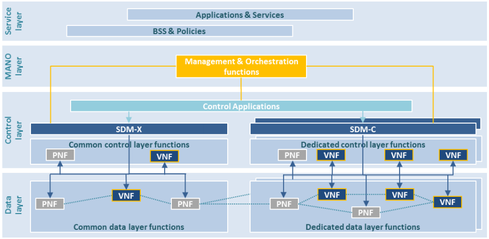
Figure 1: Architectural view of 5G networks according to 5G-PPP. Source: [3].

We remark that our work focuses on this VNF sharing problem, which is different from the one studied in traditional VNF placement studies. Fig. 2 presents a simple instance of the VNF sharing problem: the vertical has requested a new service $s_{2}$, and the SDM-X decides at which VM to run each VNF of $s_{2}$ (this decision is trivial for $v_{4}$, as there is no existing instance of it), and how to prioritize the different services sharing the same VNF.

Contributions. We make the following main contributions to the VNF-sharing problem:

• We observe that allowing flexible priorities for each VNF and service allows the MNO to meet the KPI targets at a lower cost;

• We present a system model that captures all the relevant aspects of the VNF-sharing problem and the entities it involves, including the capacity-scaling and priority-setting decisions it requires;

• leveraging convex optimization, we devise an efficient integrated solution methodology called FlexShare, which is able to make swift, high-quality decisions concerning VM usage, priority assignment, and capability scaling;

• we discuss how FlexShare can handle VNF instantiation and de-instantiation operations;

• we formally analyze the computational complexity of FlexShare and its competitive ratio relatively to the optimum;

• we study FlexShare’s performance using real-world VNF graphs.

In the rest of the paper, we begin by motivating the need for flexible priorities across VNFs (Sec. II). Then Sec. III introduces our system model and problem formulation, while Sec. IV describes the FlexShare solution strategy. Sec. V analyzes FlexShare’s performance with respect to the optimal solution. Our reference scenarios and numerical results are discussed in Sec. VI. Finally, we review related work in Sec. VII, and conclude the paper in Sec. VIII.

II The role of priorities

Before addressing the problem of whether it is convenient to share a VNF among multiple services or not, let us highlight the role of priorities while sharing a VNF instance. Three main approaches can be adopted for VNF sharing:

• per-service priority, associated with each service and constant across different VNFs;

• per-VNF priority, associated with each service and VNF, thus, given a service, it may vary across different VNFs;

• per-flow priority, associated with individual traffic flows (e.g., REST queries) belonging to a service, it may vary across the different VNFs on a per-flow basis.

In Example 1, we focus on the first two steps of the above flexibility ladder, and show how flexible priority assignment can increase the efficiency of handling service flows.

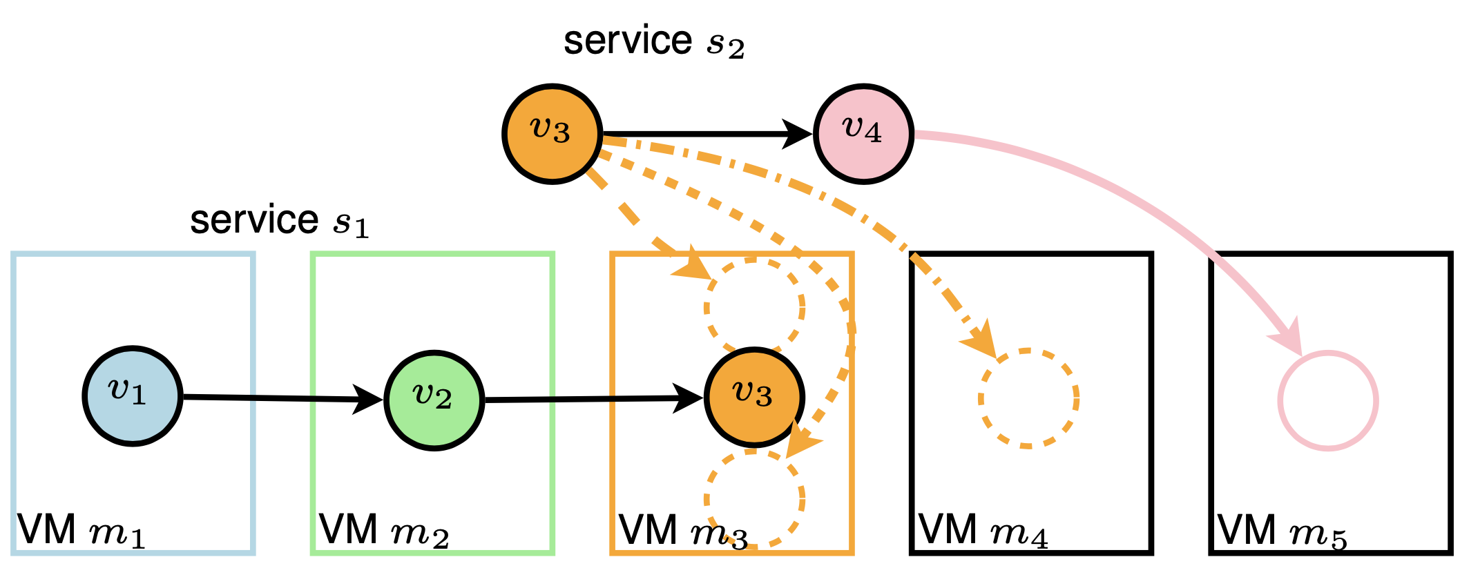
Figure 2: Example of the VNF-sharing problem. A PoP is serving service $s_{1}$, with VNFs $v_{1}$–$v_{3}$ deployed at VMs $m_{1}$–$m_{3}$. It is then requested to deploy $s_{2}$, using VNFs $v_{3}$ and $v_{4}$. No isolation is requested, so services can share VNFs if convenient. For $v_{4}$, the only option is devoting an unused VM to it, $m_{5}$ in the example (pink line). For $v_{3}$, instead, there are three options: re-using the instance of $v_{3}$ at $m_{3}$, giving $s_{2}$ a lower priority than $s_{1}$ (dashed line); doing the same but giving $s_{2}$ a higher priority (dotted line); devoting $m_{4}$ – currently unused – to $v_{3}$ (dash-dotted line), thus having two VMs running $v_{3}$.

 

Example 1 (The importance of flexible priorities).

Consider the two services, $s_{1}$ and $s_{2}$, depicted in Fig. 3, requested by a vertical specialized in video surveillance systems. Recall that services are described as VNF graphs; specifically, $s_{2}$ includes two VNFs executing transcoding and motion detection, respectively, while $s_{1}$ is composed of $s_{2}$ and a VNF performing face recognition. Each VNF should run in its own VM, and assume network transfer times between VMs are negligible. Adopting a well-established and convenient approach [7, 8], let us model VNFs as M/M/1 traffic queues processing traffic flows, and the services as queuing chains, with arrival rates $\lambda_{1}=$2\text{\,}\mathrm{f}\mathrm{l}\mathrm{o}\mathrm{w}\mathrm{s}\mathrm{/}\mathrm{m}\mathrm{s}$$, and $\lambda_{2}=$1\text{\,}\mathrm{f}\mathrm{l}\mathrm{o}\mathrm{w}\mathrm{s}\mathrm{/}\mathrm{m}\mathrm{s}$$ respectively. Also, consider service delay as the main performance metric and let the target average delay be $D^{\max}_{1}=D^{\max}_{2}=$1.1\text{\,}\mathrm{ms}$$ for both services. Then assume that when given the allocated computation resources, the service rate of the transcoding and motion detection is $\mu_{\text{tc}}=\mu_{\text{md}}=\mu=$5\text{\,}\mathrm{f}\mathrm{l}\mathrm{o}\mathrm{w}\mathrm{s}\mathrm{/}\mathrm{m}\mathrm{s}$$, while that of face recognition is $\mu_{\text{fr}}=$9.15\text{\,}\mathrm{f}\mathrm{l}\mathrm{o}\mathrm{w}\mathrm{s}\mathrm{/}\mathrm{m}\mathrm{s}$$.

To meet the delay targets, $s_{2}$ flows must traverse the transcoding and motion detection with a combined sojourn time of $1.1\text{\,}\mathrm{ms}$, while $s_{1}$ flows must do the same in at most $0.96\text{\,}\mathrm{ms}$ (i.e., the target average delay $D^{\max}_{1}$ minus the sojourn time at the face recognition VNF of $\frac{1}{\mu_{\text{fr}}-\lambda_{1}}=$0.14\text{\,}\mathrm{ms}$$). We now show that there is no way of setting per-service priorities that allow this.

Case 1: Higher priority to $s_{1}$. This choice would make intuitive sense since $s_{1}$ flows have to go through more processing stages than $s_{2}$ flows, within the same deadline. In this case, $s_{1}$ flows incur a sojourn time of $\frac{1}{\mu-\lambda_{1}}=\frac{1}{5-2}=$0.33\text{\,}\mathrm{ms}$$ for each of the common VNFs, resulting in a total delay $D_{1}=$0.8\text{\,}\mathrm{ms}$$, well within the target. However, the sojourn time of $s_{2}$ flows at each of the shared VNFs becomes [16, Sec. 3.2]: $\frac{1/\mu}{\left(1-\frac{\lambda_{1}}{\mu}\right)\left(1-\frac{\lambda_{1}+\lambda_{2}}{\mu}\right)}=\frac{1/5}{\left(1-\frac{2}{5}\right)\left(1-\frac{1+2}{5}\right)}\approx$0.83\text{\,}\mathrm{ms}$$, which results in a total delay of $D_{2}\approx$1.66\text{\,}\mathrm{ms}$>D^{\max}_{2}$.

Case 2: Higher priority to $s_{2}$. It is easy to verify that giving higher priority to $s_{2}$ implies that $s_{1}$ misses its target delay.

Case 3: Equal priority. Giving the same priority to both services results in a sojourn time of $\frac{1}{\mu-\lambda_{1}-\lambda_{2}}=\frac{1}{5-1-2}=$0.5\text{\,}\mathrm{ms}$$ for each of the common VNFs, and in a total delay of $D_{2}=$1\text{\,}\mathrm{ms}$<D^{\max}_{2}$ and $D_{1}=$1\text{\,}\mathrm{ms}$+$0.14\text{\,}\mathrm{ms}$>D^{\max}_{1}$.

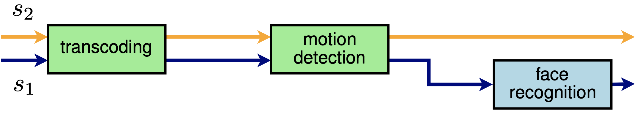
Figure 3: Example 1: two video surveillance services, $s_{1}$ and $s_{2}$, with $s_{2}$ including performing transcoding and motion detection VNFs, and $s_{1}$ composed of $s_{2}$ and an additional face recognition stage.

Flexible priorities. Assume that $s_{1}$ and $s_{2}$ have priority in the transcoding and in the motion detection VNF, respectively. Then, $D_{1}\mathord{=}\frac{1}{\mu-\lambda_{1}}\mathord{+}\frac{1/\mu}{\left(1\mathord{-}\frac{\lambda_{2}}{\mu}\right)\left(1\mathord{-}\frac{\lambda_{1}\mathord{+}\lambda_{2}}{\mu}\right)}\mathord{+}0.14\mathord{=}$ $0.33\mathord{+}0.625\mathord{+}0.14\mathord{=}$1.095\text{\,}\mathrm{ms}$<D^{\max}_{1}$, and $D_{2}\mathord{=}$ $\frac{1/\mu}{\left(1\mathord{-}\frac{\lambda_{1}}{\mu}\right)\left(1\mathord{-}\frac{\lambda_{1}\mathord{+}\lambda_{2}}{\mu}\right)}\mathord{+}\frac{1}{\mu\mathord{-}\lambda_{2}}$ $\mathord{=}0.83\mathord{+}0.25=$1.08\text{\,}\mathrm{ms}$<D^{\max}_{2}$.

  In conclusion, the above example shows that relying on merely per-service priorities may result in violation of KPI requirements. In contrast, assigning different per-VNF priorities allows the MNO to meet the vertical’s requirements while increasing efficiency in resource usage, hence lowering the costs. We later show that per-flow priorities result in even better efficiency.

III System model and problem formulation

The architecture we consider reflects real-world deployments of MEC-based networks, as described in the ETSI specifications [17]. Possible deployments differ in aspects like the location of the EPC, but all include multiple edge sites, i.e., PoPs hosting the MEC servers and some (as in Fig. 4(top)), or all (as in Fig. 4(bottom)), of the EPC network functions.

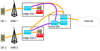
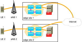
Figure 4: Two of the possible architectures for MEC-based networks discussed in [17]: distributed EPC (top) and local breakout (bottom). Orange and purple lines correspond to data and control traffic, respectively.

As mentioned, the network and computing resources available in the MEC in Fig. 4 have to be properly orchestrated and managed. In particular, referring to the 5G architecture in [4], the SDM-X has to use the VMs under its control to provide the newly-requested services with the required KPIs and at the minimum cost. It should thus make decisions on (i) whetherexisting VNF instances should to be shared; (ii) if so, how to assign the priorities to different services sharing the same VNF instance; and last (iii) scalingthe computational capabilities of the VMs if needed and possible.

We choose to focus on single PoP decisions and account for the system overheads, which, in general, are given by network delays and processing times. However, a study of the ongoing work in the datacenter networking community (see, e.g., [18]) suggests that switching is highly optimized, hence network delays are often minimal. Also, network topologies tend to be highly regular, hence delays are similar across any pair of VMs. Therefore, it is fair to neglect the network delays within a single PoP, and consider the processing times only.

Below, we describe the model and the entities that are involved in the VNF-sharing problem (Sec. III-A), followed by defining the problem objective and constraints (Sec. III-B).

III-A System model

The system model includes VMs $m\in\mathcal{M}$, and VNFs $v\in\mathcal{V}$ . Each VM runs (at most) one VNF, modeled as an M/M/1 queue with FIFO queuing and preemption, as widely assumed in recent works [7, 8, 19]. Also, let $C(m)$ be the maximum computation capability to which VM $m$ can be scaled up. We underline that, although in this work we focus on computational capability, we could adjust our model to focus on memory and storage as well. We refer to a VM as active if it hosts a VNF, and we express through binary variables $y(v,m)$ whether VM $m$ runs VNF $v$.

VNFs vary in computational requirements, which are modeled through parameter $l(v)$, expressing how many units of computational capability are needed to process one flow for VNF $v$ per time unit. For example, a VNF with requirement $l(v)=1$ running on a VM $m$ with capability $\mu(m)=1$ takes $l(v)/\mu(m)=1$ time unit to process a flow. Using the same VM for a VNF with requirement $l(v)=2$ yields a processing time of $l(v)/\mu(m)=2$ time units per flow. Note that $l(v)$ values do not depend on the actual service using VNF $v$, but on $v$ only.

Services $s\in\mathcal{S}$ include one or more VNFs, and flows belonging to service $s$ arrive at VNF $v$ with a rate $\lambda(s,v)$; VNFs that are not used by a certain service have $\lambda$-values equal to $0$. Through the $\lambda(s,v)$ parameters, we can account for arbitrarily complex service (VNF) graphs where the number of flows can change between VNFs, and some flows may visit the same VNF more than once. For sake of simplicity, in this paper we focus on the maximum average delay $D^{\max}(s)$ of service $s$ as the target KPI.

Each VM uses a quantity $\mu(m)\leq C(m)$ of computational capability that can be dynamically adjusted. Given $\mu(m)$, VNF $v$ deployed at VM $m$ processes flows at rate $\frac{\mu(m)}{l(v)}$. Finally, binary variables $x(s,v,m)$ express whether service $s$ uses the instance of VNF $v$ at VM $m$; this allows us to model the assignment of distinct services requiring the same VNF to different VMs that run the VNF. For clarity, we summarize the above parameters and variables in Tab. I.

TABLE I: Notation ($\dagger$ denotes variables of the modified problem described in Sec. IV-B)

Symbol	Type	Meaning
$\mathcal{M}=\{m\}$	Set	Set of VMs
$\mathcal{V}=\{v\}$	Set	Set of VNFs
$\mathcal{S}=\{s\}$	Set	Set of services
$C(m)$	Parameter	Maximum capability to which VM $m$ can be scaled up
$l(v)$	Parameter	Computational capability needed to process one flow unit for VNF $v$
$\lambda(s,v)$	Parameter	Arrival rate of flows of service $s$ for VNF $v$
$D^{\max}(s)$	Parameter	Target delay for service $s$
$\kappa_{f}(m)$	Parameter	Fixed cost incurred when activating VM $m$
$\kappa_{p}(m)$	Parameter	Proportional cost incurred when using one unit of computational capability for VM $m$
$p(s,v)$	Parameter	Per-VNF priority of service $s$ at VNF $v$
$\mu(m)$	Decision variable	Computational capability to use for VM $m$
$y(v,m)$	Decision variable	Whether VM $m$ runs VNF $v$
$x(s,v,m)$	Decision variable	Whether flows of service $s$ use the instance of VNF $v$ running at VM $m$
$\tilde{\Lambda}(s,v)$	Decision variable.†	Arrival rate of flows for VNF $v$ on the same VM as the one servicing $s$, that are given priority over flows of service $s$
$S(s,v)$	Auxiliary decision variable	Sojourn time of flows of service $s$ for VNF $v$
$\Lambda(s,v)$	Auxiliary decision variable	Arrival rate of flows for VNF $v$ on the same VM as the one servicing $s$, that are given priority over flows of service $s$
$\pi(s,v)$	Random variable	Describes the priority assigned to flows of service $s$ upon entering VNF $v$

III-B Problem formulation

We now discuss the objective of the VNF-sharing problem and the constraints we need to satisfy.

Objective. The high-level goal of the MNO is to minimize its incurred cost, which consists of two components: a fixed cost, $\kappa_{f}(m)$, paid if VM $m$ is activated, and a proportional cost, $\kappa_{p}(m)$, paid for each unit of computational capability used therein. The objective is then given by:

$$\min_{y,\mu}\sum_{m\in\mathcal{M}}\left(\kappa_{f}(m)\sum_{v\in\mathcal{V}}y(v,m)+\kappa_{p}(m)\mu(m)\right).$$ (1)

VM capability and VNF instances. We must account for the maximum value $C(m)$ to which the capability $\mu(m)$ of each VM $m$ can be scaled up:

$$\mu(m)\leq C(m)\quad\forall m\in\mathcal{M}.$$ (2)

Also, at most one VNF can run in any single VM:

$$\sum_{v\in\mathcal{V}}y(v,m)\leq 1,\quad\forall m\in\mathcal{M},$$ (3)

and only active VMs can be used for handling flows, i.e.,

$$y(v,m)\geq x(s,v,m),\quad\forall s\in\mathcal{S},v\in\mathcal{V},m\in\mathcal{M}.$$ (4)

Service times. Each service $s$ has a maximum average service time $D^{\max}(s)$ that must be maintained. Since we assume that processing time is the dominant component of service time, this is equivalent to imposing:

$$\sum_{v\in\mathcal{V}}S(s,v)\leq D^{\max}(s),\quad\forall s\in\mathcal{S},$$ (5)

where $S(s,v)$ is the sojourn time (i.e., the time spent waiting or being served) experienced by flows of service $s$ for VNF $v$. By convention, we set $S(s,v)=0$ if service $s$ does not require VNF $v$.

As detailed below, sojourn times, in turn, depend on:

• the computational capability $l(v)$ required for handling any flow for a VNF;

• the traffic flow arrival rate at the VNFs $\lambda(s,v)$;

• the priority of the traffic flows at the traversed VNFs (to be detailed in the sequel);

• the computational capability $\mu(m)$ assigned to the VM hosting the VNF instance processing the flow.

Using [16, Sec. 3.2] and [20], we can generalize the expression used in Example 1 and write the sojourn time of flows of service $s$ for VNF $v$ as:

$$S(s,v){=}\frac{l(v)}{\mu(\bar{m})}\frac{1}{1-l(v)\frac{\Lambda(s,v)}{\mu(\bar{m})}}\frac{1}{1-l(v)\frac{\Lambda(s,v)+\lambda(s,v)}{\mu(\bar{m})}},$$ (6)

where $\bar{m}$ is the VM hosting the instance of VNF $v$ used by service $s$, i.e., where $x(s,v,\bar{m})=1$.

In (6), $\Lambda(s,v)$ represents the arrival rate of flows (of any service) for the instance of VNF $v$ hosted on $\bar{m}$, that are given a priority higher than a generic flow of service $s$ for VNF $v$. Let $\pi(s,v)$ be the random variable describing the priority assigned to flows of service $s$ at VNF $v$, then:

$$\Lambda(s,v)=\sum_{t\in\mathcal{S}}\mathds{P}\left(\pi(t,v)>\pi(s,v)\right)\lambda(t,v).$$ (7)

The intuitive meaning of (7) is that $\Lambda(s,v)$ grows as it becomes more likely that flows of other services $t\neq s$ are given higher priority over flows of service $s$.

The expression of $\Lambda(s,v)$ depends on the type of the $\pi(s,v)$ variables. In App. A, we show how $\Lambda(s,v)$ values can be computed for the two priority assignments discussed in Sec. II, i.e., per-VNF priorities and uniform, per-flow priorities.

Problem complexity. In the general case, the expression of $\Lambda(s,v)$ is not guaranteed to be linear, convex, or even continuous. It follows that no hypothesis can be made about the complexity of the problem of setting the priorities so as to optimize (1): solving such a problem may require to search over all possible distributions of $\pi(s,v)$, which would be prohibitively complex even in small-scale scenarios.

Indeed, it is possible to reduce any instance of the bin-packing problem, which is NP-hard, to a simplified instance of our problem where (i) there is only one type of VNF, (ii) all services have the same target KPIs, and (iii) $\kappa_{p}=0$ for all VMs. Specifically:

• VMs correspond to bins;

• the capability of VMs correspond to the size of the capacity of the bin they are associated with;

• services correspond to items;

• traffic flow arrival rates $\lambda(s,v)$ correspond to the size of items.

Non-negligible network delays. As mentioned earlier, network delay within individual PoPs are very small compared to processing times, hence, our model neglects them. However, it is worth stressing that our model can be extended to account for arbitrary-delay scenarios, by introducing the following new parameters:

• for each pair $(m_{1},m_{2})$ of VMs in $\mathcal{M}$, a network delay $d(m_{1},m_{2})$;

• for each pair $(v_{1},v_{2})$ of VNFs in $\mathcal{V}$, a parameter $\rho(v_{1},v_{2})\in[0,1]$ expressing the fraction of traffic that visits $v_{2}$ immediately after visiting $v_{1}$.

Given the above parameters, the total network delay is:

$$\sum_{m_{1},m_{2}\in\mathcal{M}}\sum_{v_{1},v_{2}\in\mathcal{V}}d(m_{1},m_{2})y(v_{1},m_{1})y(v_{2},m_{2})\rho(v_{1},v_{2}).$$ (8)

Eq. (8) can be read as follows: a network delay $d(m_{1},m_{2})$ is incurred when (i) a VNF $v_{1}$ is deployed at $m_{1}$, and (ii) the subsequent VNF $v_{2}$ is deployed at $m_{2}$. The quantity in (8) should then be added to the first member of the delay constraint (5), thereby ensuring that the combination of processing and network delays is below the delay target $D^{\max}$.

IV The FlexShare solution strategy

In light of the problem complexity, we propose a fast, yet highly effective solution strategy named FlexShare, which runs iteratively and consists of four main steps as outlined in Fig. 5. The algorithm considers services one by one, adjusting its solution for every new service being deployed. The first step, detailed in Sec. IV-A, consists of building a bipartite graph including the VNFs of the new service that are to be deployed, and the VMs that are active or can be activated. The edges of the graph express the possibility of using a VM to provide a VNF, either by sharing an existing instance of the VNF or by deploying a new one. Edges are labeled with the cost associated with each decision, i.e., the $\kappa_{p}$ and/or $\kappa_{f}$ terms contributing to the objective (1). In step 2, also described in Sec. IV-A, we use the Hungarian algorithm [21] on the generated bipartite graph to get the optimal minimum-cost assignment of VNFs to VMs, i.e., the $x$- and $y$-variables.

Given these decisions, step 3 aims at assigning the priorities and finding the amount of computational capability to use in every VM. To this end, a simpler (namely, convex) variant of the problem defined in Sec. III-B is formulated and solved, as detailed in Sec. IV-B.

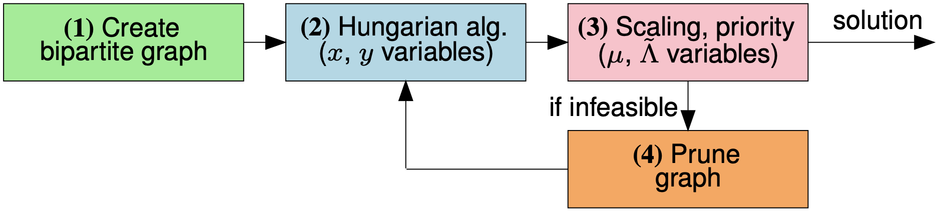
Figure 5: The FlexShare strategy. Step 1 builds a bipartite graph showing which VMs could run each VNF. Step 2 runs the Hungarian algorithm on such a graph to obtain the optimal values for the $x$- and $y$-variables. Step 3 solves a convex variant of the original problem in Sec. III-B. If feasible, its variables ($\mu$, $\tilde{\Lambda}$) are used to determine the scaling and the priorities; otherwise, the bipartite graph is pruned (step 4) and the procedure restarts from step 2.

If step 3 results in an infeasible problem, we prune the bipartite graph (step 4). The underlying intuition is that a cause for infeasibility is overly aggressive sharing of existing VNF instances. Therefore, as detailed in Sec. IV-C, we prune from the bipartite graph edges that result in an overload of VMs. After pruning, the algorithm starts a new iteration with step 2. Moving from one iteration to the next means reducing the likelihood that VNF instances are shared between services, and thus increasing the cost incurred by the MNO, due to the $\kappa_{f}$ fixed cost terms. The procedure stops as soon as it finds a feasible solution. Without loss of generality, we present FlexShare in the case where there are sufficient resources, i.e., enough VMs, to deploy all the requested services.

IV-A Steps 1–2: Bipartite graph and Hungarian algorithm

The bipartite graph. The bipartite graph represents (i) the possible VNF assignment decisions, i.e., which VNFs can be provided at which VMs and which VNFs can be shared among services, and (ii) the associated cost incurred by the MNO.

More formally, the bipartite graph is created according to the following rules:

1. a vertex is created for each VNF and for each VM;

2. an edge is drawn from every VNF to every unused VM;

3. an edge is drawn from every VNF to every VM currently running the same VNF, provided that the maximum computational capability of the VM is sufficient to guarantee stability.

Denote by $\bar{s}$ the service now being deployed. For every VNF $v$ required by $\bar{s}$, and every VM $m$ either running $v$ or not yet activated, $m$ can satisfy the request of $\bar{s}$ for $v$ while ensuring stability if

$$l(v)\sum_{s\in\mathcal{S}}\left[\left(x(s,v,m)+\mathds{1}_{s=\bar{s}}\right)\lambda(s,v)\right]<C(m),$$ (9)

i.e., if the total load on VM $m$ is no larger than its maximum capability $C(m)$.

Note that (9) does not imply that $\bar{s}$, or any other existing services, can be served in time, i.e., while satisfying their delay constraints; indeed, this depends on the priority and computational capability assignment decisions, and cannot be checked at the graph generation time. The purpose of step 1 is to generate a graph accounting for all possible assignment options, that may potentially result in a feasible solution. Fig. 6 provides an example of a bipartite graph, representing the options available in the scenario depicted in Fig. 2: VNF $v_{3}$ can be provided at VMs $m_{3}$ (which already runs $v_{3}$), or at $m_{4}$ or $m_{5}$ (which are both currently yet inactive); VNF $v_{4}$ can only be run on either $m_{4}$ or $m_{5}$.

The cost of each edge connecting VM $m$ with VNF $v$ is given by the following expression:

$$\left(1-\sum_{v}y(v,m)\right)\kappa_{f}(m)+\kappa_{p}(m)\left(l(v)\lambda(\bar{s},v)+\epsilon\right).$$ (10)

In (10), the first term is the fixed cost associated with activating VM $m$, which is incurred only if $m$ is not already active (the summation can be at most $1$, as per (3)). The second term is the proportional cost associated with the additional computation capability needed at VM $m$ to guarantee stability, with $\epsilon$ being a positive, arbitrarily small value.

Figure 6: The bipartite graph generated when trying to deploy service $s_{2}$, as shown in Fig. 2. Graph vertices correspond to VNFs in $s_{2}$ (left) and VMs (right); edges represent the possible assignment decisions. Edges connecting currently-unused VMs, i.e., $v_{4}$ and $v_{5}$, are thicker because they are associated with a higher cost (due to the $\kappa_{f}$ component).

Hungarian algorithm and assignment decisions. The Hungarian algorithm [21] is a combinatorial optimization algorithm with polynomial (cubic) time complexity in the number of edges in the graph. When applied to the bipartite graph we generate, it selects a subset of edges such that (i) each VNF is connected to exactly one VM, and (ii) the total cost of the selected edges is minimized.

Selected edges map to assignment decisions. Specifically, for each selected edge connecting VNF $v$ and VM $m$, we set $y(v,m)\leftarrow 1$ and $x(\bar{s},v,m)\leftarrow 1$, i.e., we activate $m$ (if not already active) deploying therein an instance of $v$, and use it to serve service $\bar{s}$. The obtained values for the $x$ and $y$-variables are used in step 3 to decide priorities and computational capability assignment, as set out next.

IV-B Step 3: Priority and scaling decisions

The purpose of step 3 of the FlexShare procedure is to decide the priorities to assign to each VNF and service, as well as any needed scaling of VM computation capability. Since the complexity of the problem stated in Sec. III-B depends on the presence of the $\pi(s,v)$ variables, we proceed as follows:

1. we formulate a simplified problem, which contains no random variables and is guaranteed to be convex;

2. we use the variables of the simplified problem to set the $\mu(m)$ variables of the original problem, as well as the parameters of the distribution of the $\pi(s,v)$ variables.

Convex formulation. To avoid dealing with probability distributions, we replace the $\Lambda(s,v)$ auxiliary variables of the original problem with independent variables $\tilde{\Lambda}(s,v)$, thus dispensing with (7). Given $x$ and $y$, the decision variables of the modified problem are $\tilde{\Lambda}(s,v)$ and $\mu(m)$, while the objective is still given by (1). Having $\tilde{\Lambda}(s,v)$ as a variable means deciding (intuitively) how many higher-priority traffic flows each incoming flow will find. Such values are later mapped to the parameters of the distributions of $\pi(s,v)$.

If we solve the modified problem with no further changes, the optimal solution would always yield $\tilde{\Lambda}(s,v)=0,\forall s,v$, i.e., no flow ever encounters higher-priority ones, which is clearly not realistic. To avoid that, we mandate that the average behavior, i.e., the average number of higher-priority flows met, is the same as in the original problem:

$$\sum_{s\in\mathcal{S}}\tilde{\Lambda}(s,v)=\frac{|\mathcal{S}|}{2}\sum_{s\in\mathcal{S}}\lambda(s,v),\quad\forall v\in\mathcal{V}.$$ (11)

The intuition behind (11) is that each $\Lambda(s,v)$-value (in the original problem) is the sum of several $\lambda$-values, i.e., the services arrival rates. The $\lambda$-value associated with the highest-priority service will contribute to $|\mathcal{S}|-1$ $\Lambda(s,v)$-values, the one associated with the second-highest-priority service will contribute to $|\mathcal{S}|-2$ $\Lambda(s,v)$-values, and so on. On average, each $\lambda$-value contributes to $\frac{|\mathcal{S}|}{2}$ $\Lambda(s,v)$-values. Finally, recall that $\lambda(s,v)=0$ if service $s$ does not use VNF $v$.

It can be proved that the modified problem is convex:

Property 1.

The problem of minimizing (1) subject to constraints (2)–(5) and (11), is convex.

Proof:

For the problem to be convex, the objective and all constraints must be so. Our expressions are linear, and thus convex. However, (5) contains $S(s,v)$-terms, which have to be proven to be convex. We do so by computing the second derivative of the expression $S(s,v)$ in the $\mu(m)$ and $\Lambda(s,v)$ variables. It is easy to verify that, since the quantities $\tilde{\Lambda}(s,v)$, $\mu(m)$, $\lambda(s,v)$ and $l(v)$ are all positive and the system is stable (i.e., $l(v)\Lambda(s,v)<\mu(m)$ and $l(v)(\Lambda(s,v)+\lambda(s,v))<\mu(m)$), both derivatives are positive, which proves the thesis. ∎

Note that the above property implies that the modified problem is solvable in polynomial time (in the problem size, which depends on the number of VNFs, VMs, and already-deployed services) through off-the-self, commercial solvers.

Setting the variables of the original problem. After solving the convex problem described above, we can use the optimal solution thereof to make scaling decisions, i.e., to set the $\mu(m)$ variables in the original problem, as well as the priorities, i.e., the parameters of the distribution of $\pi(s,v)$. For $\mu(m)$, we can simply use the corresponding variables in the simplified problem, which have the same meaning and are subject to the same constraints.

As far as priorities are concerned, the procedure to follow depends on the priority assignment adopted in the system at hand, hence, on the type of the variables $\pi(s,v)$. With reference to the per-VNF and per-flow priority assignments used in Sec. II and to the computations performed in Appendix A, the following holds:

• when per-VNF priorities are used, we set the $p(s,v)$ values in Appendix A in such a way that services associated with a higher $\Lambda(s,v)$ have lower priority, e.g., by imposing that $p(s,v)\leftarrow-\tilde{\Lambda}(s,v)$;

• when per-flow priorities are supported, then we can solve a system of linear equations where the $\tilde{\Lambda}(s,v)$ from the solution of the simplified problem are known terms, the $r(s,v)$ quantities are the unknowns, and equations have the form of (22) and (23) in Appendix A.

Regardless the way priorities are assigned, it is important to stress that our approach has general validity and can be combined with any type of priority distribution.

IV-C Step 4: graph pruning

If the problem we solve in step 3 (priority and scaling decisions) is infeasible, a possible cause lies in the decisions made in step 2, i.e., the $x$ and $y$ variables. Thus, we restart from step 2 considering a different bipartite graph, more likely to result in a feasible problem.

To this end, we consider the irreducible infeasible set [22] (IIS) of the problem instance solved in step 3, i.e., the set of constraints therein that, if removed, would yield a feasible problem. Given the IIS, we proceed as follows:

1. we identify constraints in the IIS of type (2), thus, a set of VMs that would need more capability;

2. among such VMs, we select those that are used by the newly-deployed service $\bar{s}$;

3. among them, we identify the one that is the closest to instability, i.e., the VM $m^{\star}$ minimizing the quantity $C(m)-\sum_{s\in\mathcal{S}}x(s,v^{\star},m)l(v^{\star})\lambda(s,v^{\star})$, where $v^{\star}$ is the VNF deployed at $m$;

4. we prune from the bipartite graph the edge $(v^{\star}$,$m^{\star})$.

The intuitive reason for this procedure is that a cause for delay constraints violations is that the newly-deployed service $\bar{s}$ is causing one of the VMs it uses to operate too close to instability, and thus with high delays. By removing the corresponding edge from the bipartite graph, we ensure that VM $m^{\star}$ is not used by service $\bar{s}$.

Note that we are guaranteed that the IIS contains at least one constraint of type (2) thanks to the following result:

Theorem 1.

Every infeasible instance of the modified problem presented in Sec. IV-B includes at least one constraint of type (2) in its IIS.

Proof:

The constraints of the modified problem are of type (2)–(5) and (11). Proving that there is a constraint of type (2) in the IIS is equivalent to proving that we can solve a violation of the other types of constraint by violating one or more constraints of type (2). Indeed, if a max-delay constraint of type (5) is violated, we can make the capacity of the VNF used by that service arbitrarily high; so doing, we can solve the violation of (5) at the cost of violating (2). Similarly, solving a violation of (11) requires increasing the $\tilde{\Lambda}$-values, which in turn increases the sojourn times and results in a violation of (5)-type constraints, thus reducing to the previous case. ∎

FlexShare then restarts with step 2, where the Hungarian algorithm takes as an input the pruned bipartite graph.

It is worth stressing that the choice of the edge to prune from the bipartite graph only depends upon the quantity $C(m)-\sum_{s\in\mathcal{S}}x(s,v^{\star},m)l(v^{\star})\lambda(s,v^{\star})$, as specified in item 3 above. Therefore, such a decision is independent on the order in which VNFs appear in the VNF graph of the service at hand.

IV-D Computational complexity

The FlexShare strategy has polynomial worst-case computational complexity. Specifically:

• step 1 involves a simple check over at most $|\mathcal{V}||\mathcal{M}|$ VNF/VM pairs;

• step 2, the Hungarian algorithm, has cubic complexity in the number of nodes in the graph [21];

• step 3 requires solving a convex problem, as proven in Property 1, and the resulting complexity is also cubic;

• step 4 iterates over at most $|\mathcal{M}|$ constraints of type (2), and thus it has linear complexity;

• the whole procedure is repeated for (at most) as many times as there are edges in the original bipartite graph.

IV-E Managing service de-instantiations

So far we have described how FlexShare deals with requests to instantiate new services. In real-world scenarios, services have a finite lifetime, hence, they will have to be de-instantiated as such a lifetime expires. This can lead to suboptimal situations, such as the one in Example 2.

 

Example 2 (The effect of de-instantiating services).

Consider three services $s_{1},\dots,s_{3}$, all including VNF $v_{1}$ and all having $\lambda(s,v_{1})=1$. Also assume that $l(v_{1})=1$ and that, in order to meet their deadlines, all services need that the service time at $v_{1}$ be lower than $S^{\max}(s,v_{1})=$1\text{\,}\mathrm{ms}$$. Finally, assume that there are two available VMs, $m_{1},m_{2}$, both having maximum capability $C(m)=5$.

Upon receiving the request for $s_{1}$, FlexShare will create an instance of $v_{1}$ in VM $m_{1}$, resulting in a service time of $S(s_{1},v_{1})=$0.25\text{\,}\mathrm{ms}$$. The same VNF instance can be used for $s_{2}$, which would get – assuming, without loss of generality, that it is assigned a lower priority – a service time of $S(s_{2},v_{1})=$0.42\text{\,}\mathrm{ms}$$. As for $s_{3}$, re-using the instance of $v_{1}$ at $m_{1}$ would result in a service time $S(s_{3},v_{1})=$1.04\text{\,}\mathrm{ms}$$, exceeding the target delay; therefore, a new instance of $v_{1}$ is created at $m_{2}$.

After its lifetime expires, service $s_{2}$ is de-instantiated, and we are left with two VMs, $m_{1}$ and $m_{2}$, both running instances of $v_{1}$. This is a suboptimal situation, since $s_{3}$ could now use the instance of $v_{1}$ at $m_{1}$, without the need to keep $m_{2}$ active.

  Situations like the one in Example 2 can happen whenever services have limited lifetimes, and cannot be avoided a priori. However, they can be effectively managed a posteriori. Specifically, we can periodically check whether there are two VMs, $m_{1},m_{2}$, and a VNF $v$ such that (i) both VMs run instances of $v$, and (ii) there exists a priority and capability assignment within $m_{1}$ such that all the services currently using the $v$ instance in $m_{2}$ can use the instance in $m_{1}$ instead, while experiencing the same service times. It is easy to see that such a check can be performed by solving a reduced version of the problem presented in Sec. IV-B, i.e., in polynomial time. If the check indicates that services ought to be moved, then FlexShare indeed moves all services currently using $m_{2}$ (i.e., $x(s,v,m_{2})=1$) to $m_{1}$ (i.e., $x(s,v,m_{1})\leftarrow 1$) and deactivates $m_{2}$ (i.e., $y(m_{2},v)\leftarrow 0$). In such a case we say that the VNF instance deployed in $m_{1}$ and that deployed in $m_{2}$ were merged into $m_{1}$. We recurrently execute this procedure as long as it reduces the overall cost, in particular, prior to processing any new service deployment request.

V Competitive analysis

In this section, we analyze FlexShare’s performance in terms of the number of activated VMs, using a simplified scenario where (i) all VMs have the same maximum capacity $C$, and (ii) it is always cheaper to increase the computation capability of an existing VM than to activate a new one, i.e., $\kappa_{f}>C\kappa_{p}$.

As FlexShare receives a sequence of service deployment requests, each requiring multiple VNFs, we analyze the competitive ratio of the algorithm at an arbitrary point within this sequence, once FlexShare has successfully processed the VNFs of all previous service requests. The following lemma shows that no two instances of the same VNF, foreseen within a FlexShare solution, could be merged in a single VM.

Lemma 1.

Consider the deployment of the services determined through FlexShare upon receiving a new service to deploy. Let $m_{1}$ and $m_{2}$ be two VMs running VNF $v$ and servings sets of services $B_{1}$ and $B_{2}$, respectively. Then any other deployment that is identical to the one produced by FlexShare, except for the fact that $B_{1}\cup B_{2}$ are both served by the same VM, is infeasible.

Proof:

We recall that sub-optimalities due to the finite services lifetime are removed in FlexShare through the procedure described in Sec. IV-E, which is run prior to every new request of service deployment. Since $\kappa_{f}>C\kappa_{p}$, if the procedure in Sec. IV-E ends up de-activating any VMs, then it necessarily reduces the cost. This implies that no two sets of service traffic flows, each set running on a different VM, can be moved and run on a single VM, since otherwise FlexShare would have performed the merge. ∎

We now focus on the feasible deployments produced by FlexShare. These necessarily meet the target delay of all services, i.e., for any service $s$, the sojourn time associated with each VNF $v$ composing the service, is such that:

$$S(s,v)=\eta(s,v)D^{\max}(s)\quad\mbox{\em s.t.}\quad\sum_{v}\eta(s,v)=1\,.$$ (12)

Note that in the above expression equality holds since, otherwise, the service deployment cost could be further reduced.

Given any delay value $d$ and VNF $v\in\mathcal{V}$, we define the load gap implied by $d$ as $\theta_{v}(d)=\sqrt{\frac{C_{v}}{d}}$, where $C_{v}=\frac{C}{l(v)}$. The following lemma shows a sufficient (but not necessary) condition for a VM to provide a delay of at most $d$ for all services sharing a VNF $v$ running on the VM.

Lemma 2 ($\theta_{v}$-load gap).

Let $v$ be a VNF that runs on VM $m$, and let $L(m,v)$ denote the load on $m$. If the normalized computation capability ($\mu(m,v)=\mu(m)/l(v)$) satisfies $L(m,v)+\theta_{v}(d)\leq\mu(m,v)\leq C_{v}$, then the sojourn time associated with any VNF $v$ composing $s$ and running on $m$, is at most $d$.

Proof:

By simple algebraic manipulation of (6), we obtain

$$\begin{array}[]{rcl}S(s,v)&=&\frac{l(v)}{\mu(m)}\frac{1}{1-l(v)\frac{\Lambda(s,v)}{\mu(m)}}\frac{1}{1-l(v)\frac{\Lambda(s,v)+\lambda(s,v)}{\mu(m)}}\\ &=&\frac{1}{\mu(m,v)}\frac{1}{1-\frac{\Lambda(s,v)}{\mu(m,v)}}\frac{1}{1-\frac{\Lambda(s,v)+\lambda(s,v)}{\mu(m,v)}}\\ &=&\mu(m,v)\frac{1}{\left(\mu(m,v)-\Lambda(s,v)\right)}\frac{1}{\left(\mu(m,v)-\Lambda(s,v)-\lambda(s,v)\right)}.\end{array}$$ (13)

By definition of $L(m,v)$ and assumption on $\mu(m,v)$,

$$\mu(m,v)-\Lambda(s,v) \geq \mu(m,v)-\Lambda(s,v)-\lambda(s,v)$$ (14)

$$\geq \mu(m,v)-L(m,v)$$ (15)

$$\geq \theta_{v}(d),$$ (16)

and also $\mu(m,v)\leq C_{v}$.

Using 14) into the equivalent of (6) shown above, we obtain that the sojourn time of flows of service $s$ for VNF $v$ running on $m$ is at most

$$\mu(m,v)\frac{1}{\left[\mu(m,v)-\Lambda(m,v)\right]^{2}}\leq C_{v}\frac{1}{\theta_{v}(d)^{2}}=d,$$ (17)

as required. ∎

For each VNF $v$, let $d_{v}=\min_{s}S(s,v)$, and let $\theta_{v}=\theta_{v}(d_{v})$. Intuitively, $d_{v}$ is the smallest sojourn time at VNF $v$ for any of the services using $v$, and $\theta_{v}$ is the load gap implied by $d_{v}$. Our competitive ratio analysis consists in showing a bound to the average load on each VM activated by FlexShare (Lemma 3). To this end, we define $N_{v}$ (resp. $N^{\star}_{v})$ to be the number of VMs running $v$ based on the decisions made by FlexShare (resp. the optimal decisions). Also, let $L_{v}$ (resp. $L^{\star}_{v}$) denote the average load in the solution produced by FlexShare (resp. the optimal solution).

Lemma 3.

If FlexShare uses more than one VM for running VNF $v$, then the average load $L_{v}$ over the VMs running VNF $v$ in FlexShare is at least $\frac{C_{v}-\theta_{v}}{2}$.

Proof:

Consider the case where FlexShare uses more than one VM for running VNF $v$. Assume by contradiction that the average load $L_{v}$ is strictly less than $\frac{C_{v}-\theta_{v}}{2}$. Consider the two least-loaded VMs in the solution produced by FlexShare. By assumption, one of them must have a load strictly less than $\frac{C_{v}-\theta_{v}}{2}$. If the sum of loads on these two VMs is less than $C_{v}-\theta_{v}$, then the services running on these two machines could have been rearranged to run on a single machine while meeting the delay constraints of all services (by the definition of $\theta_{v}$ and Lemma 2). This would however contradict Lemma 1, thereby proving the claim. ∎

Lemma 3 shows a lower bound to the load of activated VMs in FlexShare. Theorem 2 leverages this lower bound, and derives an upper bound on the competitive ratio of FlexShare in terms of the number of activated VMs. Since, in the simplified scenario we consider for our analysis, capacities and costs are the same for all VMs and $\kappa_{f}>C\kappa_{p}$, minimizing the number of active VMs also minimizes the cost function (1). There is no guarantee that this is the case in general scenarios; however, the pricing structure [23] and energy consumption [24] of real-world virtualized computing facilities do suggest that fixed cost indeed represents the main contribution to the total cost.

Theorem 2.

The competitive ratio of FlexShare in terms of the number of VMs activated for running VNF $v$ is $2+\frac{2\theta_{v}}{C_{v}-\theta_{v}}$.

Proof:

Lemma 3 shows that $N_{v}\frac{C_{v}-\theta_{v}}{2}\leq N_{v}L_{v}$ whenever at least two VMs are activated by FlexShare.

The optimal algorithm must serve the same load as FlexShare, hence: $N_{v}L_{v}=N^{\star}_{v}L^{\star}_{v}$. Furthermore, since the load of a VM cannot exceed its maximum capability, then $N^{\star}_{v}L^{\star}_{v}\leq N^{\star}_{v}C_{v}$. Combining all inequalities, we have:

$$N_{v} \leq\frac{2}{C_{v}-\theta_{v}}N^{\star}_{v}L^{\star}_{v}$$ (18)

$$\leq\frac{2C_{v}}{C_{v}-\theta_{v}}N^{\star}_{v}=\frac{2(C_{v}+\theta_{v}-\theta_{v})}{C_{v}-\theta_{v}}N^{\star}_{v}$$ (19)

$$=\left(2+\frac{2\theta_{v}}{C_{v}-\theta_{v}}\right)N^{\star}_{v}\,.$$ (20)

From (20), we obtain FlexShare’s competitive ratio in terms of VMs activated for running VNF $v$, i.e., $\frac{N_{v}}{N_{v}^{\star}}\leq 2+\frac{2\theta_{v}}{C_{v}-\theta_{v}}$. ∎

It is interesting to observe that the ratio guaranteed by Theorem 2 tends to the constant value $2$ as the maximum capability of VMs $C$ grows – a trend that is already in place, and is likely to continue as network equipment increases in computational capability.

VI Numerical results

In this section, we describe the reference scenarios and benchmark solutions we consider (Sec. VI-A), followed by our numerical results obtained under the synthetic and realistic scenarios (Sec. VI-B and Sec. VI-C, respectively), and by a discussion of the running times (Sec. VI-D).

VI-A Reference scenarios and benchmarks

TABLE II: Services in the synthetic scenario

Service	Arrival rate [flows/ms]	Max. delay [ms]
$s_{1}$	2	10
$s_{2}$	1.5	7.5
$s_{3}$	1	5

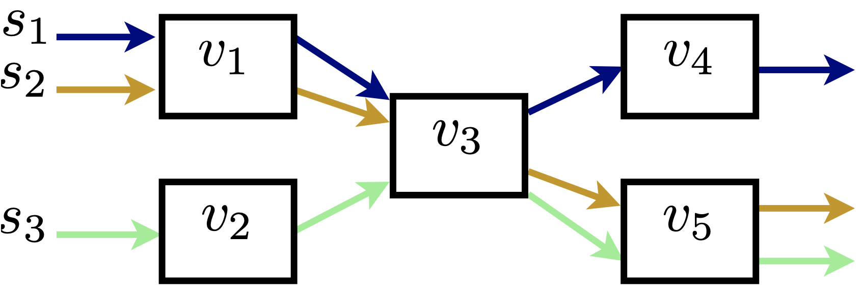
Figure 7: VNF graphs in the synthetic scenario.

Figure 8: VNF graph of the ICA service, as described in [25].

In this section, we present the two reference scenarios we consider for our performance evaluation, as well as the benchmark strategies we compare against. Without loss of generality, we consider that each service is requested exactly once, i.e., there is one service request per service.

Synthetic scenario. The synthetic scenario we use for performance evaluation includes three services $s_{1},\dots,s_{3}$, sharing five VNFs $v_{1},\dots,v_{5}$ as depicted in Fig. 7. All VNFs have coefficient $l(v)=1$, while the arrival rate and maximum delay associated with each service are summarized in Tab. II. The scenario includes $\mathcal{M}=10$ VMs whose fixed and proportional costs are $\kappa_{f}=8$ and $\kappa_{p}=0.5$ units, respectively, and whose capability is randomly distributed between 5 and 10 units.

Such a scenario is small enough to allow a comparison against optimal priority assignments found by brute-force; at the same time, it contains many interesting features, including different combinations of services sharing different VNFs and different cost/capability trade-offs.

TABLE III: Realistic scenario: traffic flow arrival rate and computational load associated with every VNF

VNF	Rate $\lambda(s,v)$	Requirement $l(v)$
Intersection Collision Avoidance (ICA)
eNB	117.69	$10^{-4}$
EPC PGW	117.69	$10^{-4}$
EPC SGW	117.69	$10^{-4}$
EPC HSS	11.77	$10^{-4}$
EPC MME	11.77	$10^{-3}$
Car information management (CIM)	117.69	$10^{-3}$
Collision detector	117.69	$10^{-3}$
Car manufacturer database	117.69	$10^{-4}$
Alarm generator	11.77	$10^{-4}$
See through (CT)
eNB	179.82	$10^{-4}$
EPC PGW	179.82	$10^{-4}$
EPC SGW	179.82	$10^{-4}$
EPC HSS	17.98	$10^{-4}$
EPC MME	17.98	$10^{-3}$
Car information management (CIM)	179.82	$10^{-3}$
CT server	179.82	5 $10^{-3}$
CT database	17.98	$10^{-4}$
Sensing (IoT)
eNB	50	$10^{-4}$
EPC PGW	50	$10^{-4}$
EPC SGW	50	$10^{-4}$
EPC HSS	5	$10^{-4}$
EPC MME	5	$10^{-3}$
IoT authentication	20	$10^{-4}$
IoT application server	20	$10^{-3}$
Smart factory (SF)
eNB	50	$10^{-4}$
EPC PGW	50	$10^{-4}$
EPC SGW	50	$10^{-4}$
EPC HSS	5	$10^{-4}$
EPC MME	5	$10^{-3}$
Robotics control	50	$10^{-3}$
Video feed from robots	5	$10^{-4}$
Entertainment (EN)
eNB	179.82	$10^{-4}$
EPC PGW	179.82	$10^{-4}$
EPC SGW	179.82	$10^{-4}$
EPC HSS	17.98	$10^{-4}$
EPC MME	17.98	$10^{-3}$
Video origin server	17.9	$10^{-3}$
Video CDN	179.82	$10^{-4}$

Realistic scenario. We consider five services, connected to the smart-city and smart-factory domains:

• Intersection Collision Avoidance (ICA): vehicles periodically broadcast a message (e.g., CAM) including their position, speed, and acceleration; a collision detector checks if any pair of them are on a collision course and, if so, it issues an alert;

• Vehicular see-through (CT): cars display on their on-board screen the video captured by the preceding vehicle, e.g., a large truck obstructing the view;

• Urban sensing, based on the Internet-of-Things (IoT);

• Smart robots: a set of robots working in a factory are controlled in real-time through the 5G network;

• Entertainment: users consume streaming contents, provided with the assistance of a content delivery network (CDN) server.

Tab. III, based on [26, 27, 28], reports the VNFs used by each service and the associated arrival rates. All services share the EPC child service, which is itself composed of five VNFs. Furthermore, the car information management (CIM) database can be shared between the ICA and the CT services. It is worth stressing that, as exemplified in Fig. 8 describing the ICA service, the VNF graphs in the realistic scenarios are not simple chains but rather generic graphs.

We leverage the mobility trace [29], combining the real-world topology of Luxembourg City with highly realistic mobility patterns. We focus on an intersection in the downtown area, and assume that all services are deployed at an edge site located at the intersection itself. Specifically,

• all vehicles within $50\text{\,}\mathrm{m}$ from the intersection are users of the ICA service, and send a packet (i.e., a CAM message) every $0.1\text{\,}\mathrm{s}$;

• all vehicles within $100\text{\,}\mathrm{m}$ from the intersection are users of the CT service, and send a packet (i.e., refresh their video) every $200\text{\,}\mathrm{ms}$, i.e., the see through video has $5\text{\,}\mathrm{f}\mathrm{p}\mathrm{s}$;

• those same vehicles use the entertainment video service, each consuming a $25\text{\,}\mathrm{f}\mathrm{p}\mathrm{s}$-video;

• a total of 200 sensors are deployed in the area, each generating, according to the traffic model described in the 3GPP standard [30], one packet every $100\text{\,}\mathrm{ms}$;

• the smart factory contains a total of 50 robots, each requiring real-time control, and 10% of which provides a video feed.

To tackle the most challenging scenario, we consider peak-time conditions, obtaining the request rates summarized in Tab. III, which also reports the load $l(v)$ associated with each VNF. As discussed in Sec. III, the $\lambda(s,v)$ values also incorporate the fact that not all flows visit all VNFs of a service, e.g., all ICA flows visit the local ICA server but only one in ten visits the remote one.

Finally, we assume that the PoP contains 10 VMs, each of which can be scaled up to at most $C(m)=$1000\text{\,}\mathrm{u}\mathrm{n}\mathrm{i}\mathrm{t}\mathrm{s}$$, and each associated with fixed and proportional costs of $\kappa_{f}=$1000\text{\,}\mathrm{u}\mathrm{n}\mathrm{i}\mathrm{t}\mathrm{s}$$ and $\kappa_{p}=$1\text{\,}\mathrm{u}\mathrm{n}\mathrm{i}\mathrm{t}$$, respectively.

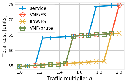
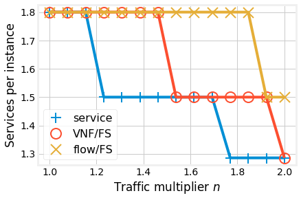
Figure 9: Synthetic scenario: total cost (left); average number of services sharing a VNF instance (center); used and maximum VM capability (right). Per-VNF and per-flow priorities are assigned via FlexShare; per-service priorities are assigned by giving higher priorities to lower-delay services.

Benchmark strategies. We study the performance of the following strategies, in increasing order of flexibility:

• service-level priorities (indicated as “service” in plots): priorities are assigned on a per-service basis, with lowest-delay services having the highest priority;

• VNF-level priorities with FlexShare (“VNF/FS”): priorities are assigned on a per-VNF basis , and FlexShare is used to determine the VNF-level priorities $p(s,v)$ (see Appendix A and Sec. IV-B);

• VNF-level priorities with brute-force (“VNF/brute”): priorities are assigned on a per-VNF basis, and all possible combinations of priorities are tested;

• flow-level priorities (“req./FS”): priorities are assigned on a per-flow level, and FlexShare is used to determine them.

Both FlexShare and the benchmark strategies are implemented in Python, and all tests are run on a Xeon E5-2640 server with 16 GByte of RAM.

VI-B Results: synthetic scenario

We start by considering the synthetic scenario and, in order to study different traffic conditions, multiply the arrival rates by a factor of $n$, ranging between 1 and 2.

Fig. 9(left) focuses on the main metric we consider, namely, the total cost incurred by the MNO. We can observe that, as one might expect, higher traffic translates into higher cost. More importantly, more flexibility in priority assignment results in substantial cost savings. As for per-VNF priorities, they exhibit an intermediate behavior between per-service and per-flow ones, with virtually no difference between the case where FlexShare is used to determine the priorities (“VNF/FS”) and that where all possible options are tried out in a brute-force fashion (“VNF/brute”). This highlights the effectiveness of the FlexShare strategy, which can make optimal decisions in almost all cases with low complexity.

Fig. 9(center) shows the average number of services sharing a VNF instance. It is clear that a higher flexibility in priority assignment results in more sharing, hence fewer VNF instances deployed. As $n$ increases, the number of services per instance decreases: scaling up (i.e., increasing the capability of VMs) is insufficient, and scaling out (i.e., increasing the number of VNF instances) becomes necessary.

This is confirmed by Fig. 9(right), depicting the total used VM capability (i.e., $\sum_{m\in\mathcal{M}}\mu(m)$) as well as the sum of the maximum values to which the capability of active VMs can be scaled up (i.e., $\sum_{m\in\mathcal{M}}C(m)y(m)$), denoted by solid and dotted lines, respectively. Both quantities grow with $n$ and decrease as flexibility becomes higher. This makes intuitive sense for the maximum capability: Fig. 9(left) shows that combining FlexShare with higher-flexibility strategies results in fewer VNF instances, hence fewer active VMs. Importantly, used capability values, i.e., $\mu(m)$, also decrease with flexibility. Indeed, higher flexibility makes it easier to match the computational capability obtained by each service within each VNF, with its needs.

Figure 10: Synthetic scenario, $n=1.8$: VNF capability compared to its maximum (i.e., maximum capability of the hosting VM) and minimum (i.e., required for stability) values. Per-VNF and per-flow priorities are assigned via FlexShare; per-service priorities are assigned by giving higher priorities to lower-delay services.

Fig. 10, obtained for $n=1.8$, provides further insights of this phenomenon. For each VNF instance deployed by each strategy, the dotted line represents the minimum capability needed by that instance to meet target delays, the dashed one corresponds to the maximum capability $C(m)$ that the VM can be scaled up to, and the solid line depicts the assigned capability $\mu(m)$. We can observe that higher-flexibility strategies correspond to assigning capability values closer to the corresponding minimum, hence, less wasted capability and lower costs. Also, note how different strategies result in different numbers of created VNF instances, from 5 with flow-level priorities (the minimum possible value, as there are five VNFs) to 7 with service-level priorities. In the latter case, two instances are created for each of $v_{3}$ and $v_{5}$, which is not unexpected as those VNFs are shared by multiple services and hence serve higher traffic (see Fig. 7).

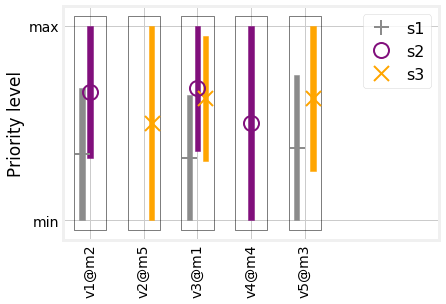
Figure 11: Synthetic scenario, $n=1.8$: priorities assigned to each service with per-service (left), per-VNF (center), and per-flow priorities (right). Per-VNF and per-flow priorities are assigned via FlexShare; per-service priorities are assigned by giving higher priorities to lower-delay services.

Fig. 11 provides a qualitative view of how priorities are assigned to different services across different VNF instances. When priorities are assigned on a per-service basis (Fig. 11(left)), services with lower target delay invariably have higher priority. If priorities are assigned on a per-VNF basis, as in Fig. 11(center), the priorities of different services can change across VNF instances, e.g., $s_{2}$ has priority over $s_{1}$ in the $v_{1}$ instance deployed at VM $m_{2}$, but the opposite happens in the $v_{3}$ instance deployed at VM $m_{1}$. Fig. 11(right) shows that if per-flow priorities are possible, services can be combined in any way at each VNF instance.

VI-C Results: realistic scenario

Figure 12: Realistic scenario: total cost (left); average number of services sharing a VNF instance (center); used and maximum VM capability (right). Per-VNF and per-flow priorities are assigned via FlexShare; per-service priorities are assigned by giving higher priorities to lower-delay services.

We now move to the realistic scenario, again multiplying the arrival rates reported in Tab. III by a factor of $n$, varying between 1 and 2. Recall that, owing to the larger scenario size, no comparison with the brute-force strategy is possible.

Fig. 12(left) shows how the total cost yielded by the different strategies has the same behavior as in the synthetic scenario (Fig. 9(left)): the higher the flexibility, the lower the cost. Furthermore, for very high values of $n$, all strategies yield the same cost; in those cases, few or no VNF instances can be shared, regardless of how priorities are assigned.

Fig. 12(center) shows that VNF instances are shared among services; by comparing it to Fig. 9(center) we can observe how the behavior of per-VNF priorities tends to be closer to per-flow priorities than to per-service ones. This suggests that, even in large and/or complex scenarios, per-VNF priorities can be a good compromise between performance and implementation complexity.

Fig. 12(right) shows a much larger difference between used and maximum capabilities compared to Fig. 9(right). This is due to the fact that, as can be seen from Tab. III, there are fewer VNFs that are common among different services, and thus fewer opportunities for sharing.

VI-D Running time

The results presented in Sec. VI-B and Sec. VI-C prove that FlexShare is effective, i.e., it is able to make high-quality (indeed, often optimal) decisions. Although its worst-case computational complexity has been proven to be polynomial in Sec. IV-D, it is natural to wonder how long FlexShare takes to make its decisions, in the two scenarios we investigate.

The results are summarized in Tab. IV: in our implementation, FlexShare never takes more than few minutes to make a decision. It is important to stress that, although such running times are already adequate for many real-world scenarios, they can be significantly reduced. Indeed, our Python implementation of FlexShare leverages the optimization routines included in the scipy library, which are themselves based on decade-old FORTRAN libraries: they are adequate for prototyping and testing, but hardly a match for commercial solvers like CPLEX and Gurobi. Furthermore, as one may expect, the realistic scenario is associated with longer solution times; intuitively, this is connected with the higher number of alternatives to explore therein.

TABLE IV: Running time (in minutes) of our FlexShare implementation, in the synthetic and realistic scenarios

Traffic multiplier	Synthetic scenario	Realistic scenario
1	4	6
1.2	5	7
1.4	6	6
1.6	5	10
1.8	7	9
2	7	12

Finally, it is interesting to note that, although the running time tends to increase with the traffic, such an increase is not monotonic. This is because the running time depends on how many times the cycle represented in Fig. 5 is executed, i.e., how many times a potentially viable deployment is found to be infeasible. This, in turn, is connected to how close to their maximum capacity VMs are, rather than to how many of them are needed.

VII Related work

5G networks based on network slicing have attracted substantial attention, with several works focusing on 5G architecture [31, 3], associated decision-making issues [32, 33], and security [34, 35].

As one of the most important decisions to make in 5G environments, VNF placement has been the focus of several studies. One popular approach is optimizing a network-centric metric, e.g., load balancing [36] or network utilization [37]. Other papers use cost functions, e.g., [38, 39], possibly including energy-efficiency considerations [40, 41]. Recent works, e.g., [42] identify energy consumption as one of the main source of operational costs (OPEX) for the MNO, and tackle it by reducing the number of idle (i.e., unused) servers.

The aforementioned works typically result in mixed-integer linear programming (MILP) models. Others cast VNF placement into a generalized assignment [43], a resource-constrained shortest path problem [44], or a set cover problem [45].

Finally, a preliminary version of this work has been published in [46]. Additions with respect to that version include a formal characterization of FlexShare’s competitive ratio, new results obtained through real-world VNF graphs, and a more detailed description of the system model.

Novelty. A first novel aspect of our work is the problem we consider, i.e., VNF-sharing within one PoP as opposed to traditional VNF placement. From the modeling viewpoint, we depart from existing works in three main ways: (i) priorities are used as a decision variable rather than as an input; (ii) different priority-assignment schemes with different flexibility are accounted for and compared; (iii) the relationship between the amount of computational resources assigned to VNFs and their performance is modeled and studied; (iv) VM capacity scaling is properly accounted for as a necessary, complementary aspect of VNF sharing.

VIII Conclusion

We have studied the VNF sharing problem where decision-making entities managing a single PoP have the option of sharing VNFs among several services requiring these VNFs. We have identified priority management as one of the key aspects of the problem, and found that higher flexibility in setting priorities translates into lower costs. In view of the above, we propose FlexShare, an efficient solution strategy able to make near-optimal decisions.

We have studied the computational complexity and competitive ratio of FlexShare, finding the former to be polynomial and the latter to be asymptotically constant as the capacity of VMs increases. Our performance evaluation, carried out with reference to real-world VNF graphs, has highlighted how FlexShare consistently outperforms state-of-the-art alternatives, and that higher flexibility in setting priority always yields lower costs.

Appendix A Computing $\Lambda(s,v)$ for relevant priority assignments

The quantity $\Lambda(s,v)$, defined in Sec. III-B, represents the arrival rate of traffic flows (of any service) arriving at VNF $v$, whose priority is higher than a generic flow of service $s$ arriving at the same VNF $v$. In the following, we show how such quantities can be computed under the two priority assignments discussed in Example 1, i.e., per-VNF priorities and uniformly-distributed, per-flow priorities.

A-A Per-VNF priorities

We recall that, if per-VNF priorities are supported as in Sec. II, then all flows of each service $s$ for VNF $v$ are given the same deterministic priority, which we denote by $p(s,v)$. Thus, in the per-VNF case, $\pi(s,v)$ is always distributed according to a Dirac delta function centered in $p(s,v)$, i.e., $\delta\left(\pi(s,v)-p(s,v)\right)$. Hence, $\Lambda(s,v)$ is discontinuous and given by:

$$\Lambda(s,v)=\sum_{t\in\mathcal{S}}H\left(p(t,v)-p(s,v)\right)\lambda(t,v),$$ (21)

where $H(\cdot)$ is the Heaviside step function. Indeed, intuitively a flow of service $s$ will be queued after all flows of services $t$ with higher priority than $s$ (since $H(p(t,v)-p(s,v))=1$ if $p(t,v)>p(s,v)$), after half of the flows of services with the same priority as $s$ (since $H(p(t,v)-p(s,v))=0.5$ if $p(t,v)=p(s,v)$), and before all other flows (since $H(p(t,v)-p(s,v))=0$ if $p(t,v)<p(s,v)$).

A-B Per-flow priorities

This case corresponds to higher flexibility and implies that priorities could follow any distribution. Below, we focus on the simple, yet relevant, case where priorities are distributed uniformly between $r(s,v)-j$ and $r(s,v)+j$. In this case, let us define the quantity $q(s,t,v)=\mathds{P}(\pi(t,v)>\pi(s,v))$, whose value can be computed through the convolution of the pdfs of $\pi(s,v)$ and $\pi(t,v)$. Through algebraic manipulations [diffvar] we get:

$$\begin{aligned} q(s,t,v)&=\mathds{P}(\pi(t,v)>\pi(s,v))\\ &=\mathds{P}\left(\pi(t,v)-\pi(s,v)>0\right)\\ \end{aligned}\\ =\begin{cases}1&\text{if }r(t,v){-}r(s,v)>2j\\ \frac{1}{2}{+}\frac{r(t,v)-r(s,v)}{4j}&\text{if }-2j{\leq}r(t,v){-}r(s,v){\leq}2j\\ 0&\text{if }r(t,v){-}r(s,v)<-2j\,.\end{cases}$$ (22)

Once the $q(s,t,v)$ are known, the $\Lambda(s,v)$ values can be computed by replacing (22) in (7), obtaining:

$$\Lambda(s,v)=\sum_{t\in\mathcal{S}}q(s,t,v)\lambda(t,v).$$ (23)

We can further prove that, in this case, the choice of the variation $j$ to use in defining the variable $\pi(s,v)$ has no influence on the possible decisions.

Property 2.

If per-flow, uniformly-distributed priorities are used, then the choice of the variation $j$ has no impact over the solution space.

Proof:

The variation $j$ only appears in the $q(s,t,v)$ quantity used in (22); thus, proving the property is equivalent to showing that, if it is possible to obtain a certain value of $q(s,t,v)$ with a certain variation $j_{1}$, then it is possible to obtain the same value with any other variation $j_{2}\neq j_{1}$.

We provide a constructive proof of this, showing that scaling all per-VNF priorities $p(s,v)$ by $\frac{j_{2}}{j_{1}}$ yields the same values of $q(s,t,v)$, hence the same decisions. Focusing on the second case of (22), and re-writing $j_{2}$ as $\frac{j_{2}}{j_{1}}j_{1}$, we have:

$$\frac{\frac{2\frac{j_{2}+j_{2}}{j_{1}}r(t,v)-\frac{j_{2}}{j_{1}}r(s,v)}{j_{1}}j_{1}}{4\frac{j_{2}}{j_{1}}j_{1}}=\frac{2j_{1}+r(t,v)-r(s,v)}{4j_{1}}.$$

∎

References

- [1] D. Meisner, B. T. Gold, and T. F. Wenisch, “PowerNap: eliminating server idle power,” in ACM sigplan notices, 2009.
- [2] NGMN Alliance, “Description of network slicing concept,” 2016.
- [3] P. Rost, C. Mannweiler, D. S. Michalopoulos, C. Sartori, V. Sciancalepore, N. Sastry, O. Holland, S. Tayade, B. Han, D. Bega et al., “Network slicing to enable scalability and flexibility in 5G mobile networks,” IEEE Comm. Mag., 2017.
- [4] 5G PPP Architecture Working Group, “View on 5G Architecture,” 2017.
- [5] IETF, “Network Slicing Management and Orchestration,” 2017.
- [6] J. Cao, Y. Zhang, W. An, X. Chen, Y. Han, and J. Sun, “VNF Placement in Hybrid NFV Environment: Modeling and Genetic Algorithms,” in IEEE ICPADS, 2016.
- [7] R. Cohen, L. Lewin-Eytan, J. S. Naor, and D. Raz, “Near optimal placement of virtual network functions,” in IEEE INFOCOM, 2015.
- [8] S. Agarwal, F. Malandrino, C.-F. Chiasserini, and S. De, “Joint VNF Placement and CPU Allocation in 5G,” in IEEE INFOCOM, 2018.
- [9] G. Einziger, M. Goldstein, and Y. Sa’ar, “Faster placement of virtual machines through adaptive caching,” in IEEE INFOCOM, 2019.
- [10] ETSI, “Network Functions Virtualisation (NFV); Management and Orchestration,” 2014.
- [11] ——, “Network Functions Virtualisation (NFV); Management and Orchestration; Or-Vnfm reference point – Interface and Information Model Specification,” 2016.
- [12] K. Antevski, J. Martín-Pérez, N. Molner, C. F. Chiasserini, F. Malandrino, P. A. Frangoudis, A. Ksentini, X. Li, J. X. Salvat, R. Martinez, I. Pascual, J. Mangues-Bafalluy, J. Baranda, B. Martini, and M. Gharbaoui, “Resource orchestration of 5G transport networks for vertical industries,” in IEEE PIMRC, 2018.
- [13] B. Sayadi, M. Gramaglia, V. Friderikos, D. von Hugo, P. Arnold, M.-L. Alberi-Morel, M. A. Puente, V. Sciancalepore, I. Digon, and M. R. Crippa, “SDN for 5G Mobile Networks: NORMA perspective,” in Springer CROWNCOM, 2016.
- [14] A. De la Oliva, X. Li, X. Costa-Perez, C. J. Bernardos, P. Bertin, P. Iovanna, T. Deiss, J. Mangues, A. Mourad, C. Casetti et al., “5g-transformer: Slicing and orchestrating transport networks for industry verticals,” IEEE Communications Magazine, 2018.
- [15] NGMN Alliance, “5G Network and Service Management including Orchestration,” 2017.
- [16] L. Kleinrock, Queueing systems: Computer applications. John Wiley & Sons, 1976.
- [17] ETSI, “MEC Deployments in 4G and Evolution Towards 5G,” 2018.
- [18] W. Xia, P. Zhao, Y. Wen, and H. Xie, “A survey on data center networking (DCN): Infrastructure and operations,” IEEE Comm. surveys & tutorials, 2017.
- [19] D. Bhamare, M. Samaka, A. Erbad, R. Jain, L. Gupta, and H. A. Chan, “Optimal virtual network function placement in multi-cloud service function chaining architecture,” Computer Communications, 2017.
- [20] Malathi Veeraraghavan. (2014) Priority queueing. http://www.ece.virginia.edu/mv/edu/715/lectures/PQ.pdf.
- [21] H. W. Kuhn, “The hungarian method for the assignment problem,” Wiley Naval Research Logistics, 1955.
- [22] J. W. Chinneck, Feasibility and Infeasibility in Optimization:: Algorithms and Computational Methods. Springer, 2007.
- [23] Amazon. AWS Greengrass. https://aws.amazon.com/greengrass/.
- [24] Intel. Power Management States: P-States, C-States, and Package C-States. https://software.intel.com/en-us/articles/power-management-states-p-states-c-states-and-package-c-states.
- [25] Q.-H. Nguyen, M. Morold, K. David, and F. Dressler, “Adaptive Safety Context Information for Vulnerable Road Users with MEC Support,” in IEEE/IFIP WONS, 2019.
- [26] C. Casetti, C. F. Chiasserini, N. Molner, J. Martin-Perez, T. Deiss, C.-T. Phan, F. Messaoudi, G. Landi, and J. B. Baranzano, “Arbitration among vertical services,” in IEEE PIMRC, 2018.
- [27] T. Taleb, A. Ksentini, and A. Kobbane, “Lightweight mobile core networks for machine type communications,” IEEE Access, 2014.
- [28] T. Taleb, I. Afolabi, and M. Bagaa, “Orchestrating 5g network slices to support industrial internet and to shape next-generation smart factories,” IEEE Network, 2019.
- [29] L. Codeca, R. Frank, and T. Engel, “Luxembourg SUMO Traffic (LuST) Scenario: 24 hours of mobility for vehicular networking research,” in IEEE VNC, 2015.
- [30] 3GPP, “3GPP specification: 37.868; RAN improvements for machine-type communications,” Tech. Rep., 2014.
- [31] H. Zhang, N. Liu, X. Chu, K. Long, A.-H. Aghvami, and V. C. Leung, “Network slicing based 5G and future mobile networks: mobility, resource management, and challenges,” IEEE Comm. Mag., 2017.
- [32] K. Samdanis, S. Wright, A. Banchs, A. Capone, M. Ulema, and K. Obana, “5G Network Slicing – Part 2: Algorithms and practice,” IEEE Comm. Mag., 2017.
- [33] S. Vassilaras, L. Gkatzikis, N. Liakopoulos, I. N. Stiakogiannakis, M. Qi, L. Shi, L. Liu, M. Debbah, and G. S. Paschos, “The algorithmic aspects of network slicing,” IEEE Comm. Mag., 2017.
- [34] M. A. S. Santos, A. Ranjbar, G. Biczók, B. Martini, and F. Paolucci, “Security requirements for multi-operator virtualized network and service orchestration for 5g,” in Guide to Security in SDN and NFV. Springer, 2017.
- [35] X. Li, J. Mangues-Bafalluy, I. Pascual, G. Landi, F. Moscatelli, K. Antevski, C. J. Bernardos, L. Valcarenghi, B. Martini, C. F. Chiasserini et al., “Service orchestration and federation for verticals,” in IEEE WCNC Workshops, 2018.
- [36] A. Hirwe and K. Kataoka, “LightChain: A lightweight optimization of VNF placement for service chaining in NFV,” in IEEE NetSoft, 2016.
- [37] T. W. Kuo, B. H. Liou, K. C. J. Lin, and M. J. Tsai, “Deploying chains of virtual network functions: On the relation between link and server usage,” in IEEE INFOCOM, 2016.
- [38] M. Mechtri, C. Ghribi, and D. Zeghlache, “A scalable algorithm for the placement of service function chains,” IEEE Trans. on Network and Service Management, 2016.
- [39] L. Gu, S. Tao, D. Zeng, and H. Jin, “Communication cost efficient virtualized network function placement for big data processing,” in IEEE INFOCOM Workshops, 2016.
- [40] A. Marotta and A. Kassler, “A power efficient and robust virtual network functions placement problem,” in IEEE ITC, 2016.
- [41] N. E. Khoury, S. Ayoubi, and C. Assi, “Energy-Aware Placement and Scheduling of Network Traffic Flows with Deadlines on Virtual Network Functions,” in IEEE CloudNet, 2016.
- [42] C. Pham, N. H. Tran, S. Ren, W. Saad, and C. S. Hong, “Traffic-aware and energy-efficient vnf placement for service chaining: Joint sampling and matching approach,” IEEE Transactions on Services Computing, 2017.
- [43] R. Cohen, L. Lewin-Eytan, J. S. Naor, and D. Raz, “Near optimal placement of virtual network functions,” in IEEE INFOCOM, 2015.
- [44] B. Martini, F. Paganelli, P. Cappanera, S. Turchi, and P. Castoldi, “Latency-aware composition of virtual functions in 5G,” in IEEE NetSoft, 2015.
- [45] A. Tomassilli, F. Giroire, N. Huin, and S. Pérennes, “Provably efficient algorithms for placement of service function chains with ordering constraints,” in IEEE INFOCOM, 2018.
- [46] F. Malandrino and C. F. Chiasserini, “Getting the most out of your VNFs: flexible assignment of service priorities in 5G,” in IEEE WoWMoM, 2019.