Investigating the multiwavelength behaviour of the flat spectrum radio quasar CTA 102 during 2013–2017

Abstract

We present a multiwavelength study of the flat-spectrum radio quasar CTA 102 during 2013–2017. We use radio-to-optical data obtained by the Whole Earth Blazar Telescope, 15 GHz data from the Owens Valley Radio Observatory, 91 and 103 GHz data from the Atacama Large Millimeter Array, near-infrared data from the Rapid Eye Monitor telescope, as well as data from the Swift (optical-UV and X-rays) and Fermi ($\gamma$ rays) satellites to study flux and spectral variability and the correlation between flux changes at different wavelengths. Unprecedented $\gamma$-ray flaring activity was observed during 2016 November–2017 February, with four major outbursts. A peak flux of (2158 $\pm$ 63)$\times$10^-8 ph cm^-2 s^-1, corresponding to a luminosity of (2.2 $\pm$ 0.1)$\times$10⁵⁰ erg s^-1, was reached on 2016 December 28. These four $\gamma$-ray outbursts have corresponding events in the near-infrared, optical, and UV bands, with the peaks observed at the same time. A general agreement between X-ray and $\gamma$-ray activity is found. The $\gamma$-ray flux variations show a general, strong correlation with the optical ones with no time lag between the two bands and a comparable variability amplitude. This $\gamma$-ray/optical relationship is in agreement with the geometrical model that has successfully explained the low-energy flux and spectral behaviour, suggesting that the long-term flux variations are mainly due to changes in the Doppler factor produced by variations of the viewing angle of the emitting regions. The difference in behaviour between radio and higher energy emission would be ascribed to different viewing angles of the jet regions producing their emission.

1 Introduction

Blazars are an extreme class of active galactic nuclei (AGN) whose bright and violently variable non-thermal radiation across the entire electromagnetic spectrum is ascribed to the presence of a collimated relativistic jet closely aligned to our line of sight (e.g., Blandford $\&$ Rees, 1978). This peculiar setting implies a strong amplification of the rest-frame radiation because of Doppler boosting, together with a contraction of the variability time-scales, and a blueshift of the frequencies.

The relativistic jets of blazars are able to transport a huge amount of power away from the central engine in the form of radiation, kinetic energy, and magnetic fields. When this power is dissipated, the particles emit the observed radiation, showing the typical double-hump spectral energy distribution (SED) of blazars. The first peak of the SED, usually observed between radio and X-rays, is due to the synchrotron radiation from relativistic electrons, while the second peak, usually observed from X-ray up to TeV energies, is commonly interpreted as inverse Compton (IC) scattering of seed photons, either internal or external to the jet, by highly relativistic electrons. However, the nature of this second hump is a controversial issue and other models involving hadronic and lepto-hadronic processes have been proposed (e.g., Böttcher et al., 2013).

Blazars are traditionally divided into flat-spectrum radio quasars (FSRQ) and BL Lac objects (BL Lacs), based on the presence or not, respectively, of broad emission lines (i.e., equivalent width $>$ 5 Å) in their optical and UV spectrum (e.g., Stickel et al., 1991). Recently, a new classification was proposed based on the luminosity of the broad-line region (BLR) in Eddington luminosity (Ghisellini et al., 2011): sources with $L_{BLR}$/$L_{Edd}$ higher or lower than 5$\times$10^-4 being classified as FSRQ or BL Lacs, respectively, in agreement with a transition of the accretion regime from efficient to inefficient between the two classes.

Blazar emission shows strong and unpredictable variability over all the electromagnetic spectrum, from the radio band to $\gamma$ rays, with time-scales ranging from minutes to years. Long-term observations of blazars during different activity states provide an ideal laboratory for investigating the emission mechanisms at work in this class of sources. In this paper we present multifrequency observations of the blazar CTA 102 during 2013–2017. CTA 102 (also known as 4C $+$11.69) is an FSRQ at redshift $z=1.037$ (Schmidt, 1965). Flaring activity in the optical band has been observed from this source in 1978 (Pica et al., 1988), 1996 (Katajainen et al., 2000), and 2004 (Osterman Meyer, 2009). However, simultaneous $\gamma$-ray observations were not available for those events. The source was detected for the first time in $\gamma$ rays by the Compton Gamma Ray Observatory in 1992 with both the EGRET (Hartman et al., 1999) and COMPTEL (Blom et al., 1995) instruments. Unfortunately, no optical observations were available during the $\gamma$-ray detection (Villata et al., 1997). On the other hand, during the Fermi era a remarkable outburst was simultaneously observed in 2012 September–October in near-infrared (near-IR) and optical bands by the Whole Earth Blazar Telescope (WEBT) and $\gamma$ rays by the Large Area Telescope (LAT) on board Fermi Gamma-ray Space Telescope. Correlated variability in the two energy bands suggested a co-spatial origin of the optical and $\gamma$-ray emitting regions during the flaring activity (Larionov et al., 2016).

In 2016 November, CTA 102 entered a new very-high-activity state in $\gamma$ rays, as observed by Fermi-LAT, reaching a daily flux higher than 1$\times$10^-5 ph cm^-2 s^-1 on 2016 December 16 (Ciprini et al., 2016). This flaring activity continued for a few weeks in $\gamma$ rays (e.g., Bulgarelli et al., 2016; Xu et al., 2016). A significant increase of activity was observed over the entire electromagnetic spectrum (e.g., Calcidese et al., 2016; Ojha et al., 2016; Righini et al., 2016). In particular, an extreme optical and near-IR outburst occurred in 2016 December, with a brightness increase up to six magnitudes with respect to the faint state of the source (Raiteri et al., 2017). In Raiteri et al. (2017) we explained the flux and spectral variations in optical, near-IR, and radio bands by means of an inhomogeneous curved jet with different jet regions changing their orientation, and hence their Doppler factors, in time. Alternative theoretical scenarios have been proposed to explain the 2016–2017 flaring behaviour of CTA 102. According to Casadio et al. (2019) the outburst was produced by a superluminal component crossing a recollimation shock, while for Zacharias et al. (2017, 2019) it was due to ablation of a gas cloud penetrating the relativistic jet in a leptonic or hadronic scenario.

The radio-to-optical and $\gamma$-ray emission are produced by two different mechanisms (i.e. synchrotron and IC emission in leptonic models), although related to the same relativistic electron population. Therefore, the $\gamma$-ray variability can be used as a further test to verify the geometrical model that we proposed to explain the low-energy flux variability in CTA 102 during 2013–2017. In the geometrical scenario, the $\gamma$-ray and optical radiation are produced in the same jet region, therefore the $\gamma$-ray and optical fluxes undergo the same Doppler beaming and should be linearly correlated.

In this paper we present a multiwavelength analysis of the CTA 102 emission from radio to $\gamma$ rays between 2013 January 1 and 2017 February 9, in particular during the bright flaring activity occurred during 2016 November–2017 February. The radio-to-optical observations performed in the framework of a campaign led by the WEBT, already presented in Raiteri et al. (2017), are complemented by the Atacama Large millimeter/Submillimeter Array (ALMA) at 91 and 103 GHz, the Owens Valley Radio Observatory (OVRO) data at 15 GHz, the Rapid Eye Mount (REM) near-IR data, and a detailed analysis of data collected by the Neil Gehrels Swift Observatory (optical–UV and X rays) and Fermi ($\gamma$ rays) satellites. The data set used in this paper is the richest in terms of number of data points and broad-band coverage presented in literature for the period considered here.

Sun constraints prevented us to have observations from optical and near-infrared WEBT observatories and Swift satellite after 2017 February 9, not allowing us to investigate the connection between the $\gamma$-ray flaring activity observed in 2017 March–April (see e.g., Shukla et al., 2018) and the emission from near-IR to X-rays. After that period the infrared-to-X-ray coverage is insufficient to adequately test the geometrical model and to investigate the connection between low-energy and $\gamma$-ray emission.

The paper is organized as follows. In Section 2 and 3 we present Fermi-LAT and Swift data analysis and results, respectively, whereas in Section 4 we report on the radio-to-optical observations. Multifrequency flux and spectral variability are discussed in Sections 5 and 6, respectively. The application of the geometrical model by Raiteri et al. (2017) to the $\gamma$-ray, optical, and radio variability is discussed in Section 7. We discuss the previous results and draw our conclusions in Section 8. Throughout this paper, we assume the following cosmology: $H_{0}=71\;{\rm km\;s^{-1}\;Mpc^{-1}}$, $\Omega_{\rm M}=0.27$, and $\Omega_{\rm\Lambda}=0.73$ in a flat Universe (Ade et al., 2016).

2 Fermi-LAT Data: analysis and results

Figure 1: Integrated flux light curve of CTA 102 (upper panel), spectral slope (middle panel), curvature parameter (bottom panel) obtained in the 0.1–300 GeV energy range during 2013 January 1–2017 February 9 (MJD 56293–57793) with 30-d time bins. The open symbols refer to results obtained with $\beta$ fixed to 0.07 (see the text for details).

The Fermi-LAT is a pair-conversion telescope operating from 20 MeV to $>$ 300 GeV. Further details about the Fermi-LAT are given in Atwood et al. (2009).

The LAT data used in this paper were collected from 2013 January 1 (MJD 56293) to 2017 February 9 (MJD 57793). During this time, the LAT instrument operated almost entirely in survey mode. The Pass 8 data (Atwood et al., 2013), based on a complete and improved revision of the entire LAT event-level analysis, were used. The analysis was performed with the ScienceTools software package version v11r5p3. Only events belonging to the ‘Source’ class (evclass=128, evtype=3) were used. We selected only events within a maximum zenith angle of 90 deg to reduce contamination from the Earth limb $\gamma$ rays, which are produced by cosmic rays interacting with the upper atmosphere. The spectral analysis was performed with the instrument response functions P8R2_SOURCE_V6 using a binned maximum-likelihood method implemented in the Science tool gtlike. Isotropic (‘iso_source_v06.txt’) and Galactic diffuse emission (‘gll_iem_v06.fit’) components were used to model the background (Acero et al., 2016). The normalization of both components was allowed to vary freely during the spectral fitting.

We analysed a region of interest of $20^{\circ}$ radius centred at the location of CTA 102. We evaluated the significance of the $\gamma$-ray signal from the source by means of a maximum-likelihood test statistic (TS) defined as TS = 2$\times$(log$L_{1}$ - log$L_{0}$), where $L$ is the likelihood of the data given the model with ($L_{1}$) or without ($L_{0}$) a point source at the position of CTA 102 (e.g., Mattox et al., 1996). The source model used in gtlike includes all the point sources from the 3FGL catalogue that fall within $30^{\circ}$ of CTA 102. We also included new candidates within $10^{\circ}$ of CTA 102 from a preliminary eight-year point source list (FL8Y). The spectra of these sources were parametrized by a power law (PL), a log-parabola (LP), or a super exponential cut-off, as in the catalogues.

A first maximum-likelihood analysis was performed over the whole period to remove from the model the sources having TS $<25$. A second maximum-likelihood analysis was performed on the updated source model. In the fitting procedure, the normalization factors and the spectral parameters of the sources lying within 10^∘ of CTA 102 were left as free parameters. For the sources located between 10^∘ and 30^∘ from our target, we kept the normalization and the spectral shape parameters fixed to the values from the 3FGL catalogue.

Integrating over 2013 January 1–2017 February 9 the fit with an LP model, $dN/dE\propto$ $E/E_{0}^{-\alpha-\beta\,\log(E/E_{0})}$, as in the 3FGL and FL8Y catalogues, results in TS = 125005 in the 0.1–300 GeV energy range, with an integrated average flux of (93.8 $\pm$ 0.6)$\times$10^-8 ph cm^-2 s^-1, a spectral slope $\alpha$ = 2.16 $\pm$ 0.01 at the reference energy $E_{0}$ = 308 MeV, and a curvature parameter around the peak $\beta$ = 0.07 $\pm$ 0.01. The corresponding apparent isotropic $\gamma$-ray luminosity is (5.1 $\pm$ 0.1) $\times$10⁴⁸ erg s^-1. As a comparison in the 3FGL catalogue, covering the period 2008 August 4–2012 July 31, the integrated average flux is (16.1 $\pm$ 0.5)$\times$10^-8 ph cm^-2 s^-1, and the spectrum is described by an LP with a spectral slope $\alpha$ = 2.34 $\pm$ 0.03 at the reference energy $E_{0}$ = 308 MeV, and a curvature parameter around the peak $\beta$ = 0.13 $\pm$ 0.02. This indicates a moderate change of the average $\gamma$-ray spectrum during the period studied here, in which the flux is a factor of approximately six higher than the first four years of LAT operation.

Fig. 1 shows the $\gamma$-ray flux (top panel) and spectral parameters (middle panel: spectral slope; bottom panel: curvature parameter) evolution of CTA 102 for the period 2013 January 1–2017 February 9 using an LP model and 30-d time bins. For each time bin, the spectral parameters of both CTA 102 and all sources within 10^∘ from it were left free to vary. For the time bins in which the fit results in a TS $<$ 300 for CTA 102, the statistics is not enough for obtaining a detailed characterization of the spectrum with complex spectral models, therefore we run again the likelihood analysis using an LP model with the curvature parameter fixed to the value obtained integrating over the entire period (i.e $\beta$ = 0.07). The $\gamma$-ray spectrum of CTA 102 shows a remarkable variability on monthly time-scale, with a spectral slope between 1.88 and 2.97 (the average spectral slope is $\langle\alpha\rangle$ = 2.30 $\pm$ 0.09), and a curvature parameter between 0.04 and 0.26 (the average curvature parameter is $\langle\beta\rangle$ = 0.13 $\pm$ 0.04), although for the latter the uncertainties are relatively large.

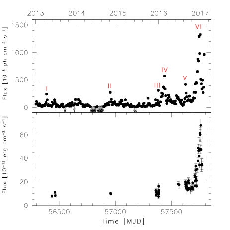
Figure 2: Upper panel: Integrated flux light curve of CTA 102 obtained in the 0.1–300 GeV energy range during 2013 January 1–2017 February 9 with five-day time bins. The arrow refers to 2$\sigma$ upper limit on the source flux. Upper limits are computed when TS $<$ 10. Different outbursts are labelled with an identification number in the plot. Bottom panel: X-ray light curve in the 0.3–10 keV energy range obtained by Swift-XRT (see Section  3 for details).

Figure 3: Integrated flux light curve of CTA 102 obtained by Fermi-LAT in the 0.1–300 GeV energy range during 2016 November 11–2017 February 9, with one-day time bins (top panel), and 12-h time bins (bottom panel).

For investigating the $\gamma$-ray variability on different time-scales, we have produced a $\gamma$-ray light curve for the entire period with five-day time bins (Fig. 2). For each time bin, the spectral parameters of CTA 102 and all sources within 10^∘ of it were frozen to the values resulting from the likelihood analysis over the respective monthly time bin. When TS $<$ 10, 2$\sigma$ upper limits were calculated. Six peaks corresponding to periods with fluxes higher than 2$\times$10^-6 ph cm² s^-1 were observed in 2013 April 4–8 (MJD 56386–56390; I), 2014 October 21–25 (MJD 56951–56955; II), 2015 December 26–30 (MJD 57382–57386; III), 2016 February 19–23 (MJD 57437–57441; IV), 2016 August 22–26 (MJD 57622–57626; V), and 2016 December 30–2017 January 3 (MJD 57752–57756; VI), with an increase of the flux of a factor between 2.5 and 14 with respect to the average flux estimated during 2013–2017.

Finally, we have produced a $\gamma$-ray light curve with one-day and 12-h time bins for the period of high activity, i.e. 2016 November 11–2017 February 9 (MJD 57703–57793), as shown in Fig. 3. In the analysis of the sub-daily light curves, we fixed the flux of the diffuse emission components at the value obtained by fitting the data over the entire period analysed in this paper. For each time bin, the spectral parameters of both CTA 102 and all sources within 10^∘ of it were frozen to the values resulting from the likelihood analysis in the monthly time bins. The peak flux of the daily light curve dates 2016 December 28 (MJD 57750), with a flux of (2158 $\pm$ 63)$\times$10^-8 ph cm^-2 s^-1, corresponding to a $\gamma$-ray luminosity (2.2 $\pm$ 0.1) $\times$10⁵⁰ erg s^-1. A similar peak flux was observed on 12-h time-scales, (2200 $\pm$ 111)$\times$10^-8 ph cm^-2 s^-1 in the second bin of 2016 December 28, corresponding to a $\gamma$-ray luminosity (2.2 $\pm$ 0.1) $\times$10⁵⁰ erg s^-1. These values are among the highest $\gamma$-ray luminosities ever measured for blazars, comparable to what was observed for 3C 454.3 (Abdo et al., 2011) and S5 0836$+$710 (Orienti et al., 2019). As a comparison, in 2012 the $\gamma$-ray flux of CTA 102 reached a peak flux of $\sim$9 $\times$10^-6 ph cm^-2 s^-1 (Larionov et al., 2016).

The search for variability on very short time-scale in $\gamma$ rays is beyond the scope of this paper. Rapid variability on time-scale of minutes was observed in 2016 December, with a peak flux of $\sim$3.5 $\times$10^-5 ph cm^-2 s^-1 (Gasparyan et al., 2018; Shukla et al., 2018; Meyer et al., 2019).

3 Neil Gehrels Swift Observatory data: analysis and results

The Neil Gehrels Swift Observatory satellite (Gehrels et al., 2004) carried out 73 observations of CTA 102 between 2013 March 24 (MJD 56436) and 2017 January 18 (MJD 57771). The observations were performed with all three instruments on board: the X-ray Telescope (XRT; Burrows et al., 2005, 0.2–10.0 keV), the Ultraviolet/Optical Telescope (UVOT; Roming et al., 2005, 170–600 nm), and the Burst Alert Telescope (BAT; Barthelmy et al., 2005, 15–150 keV).

The hard X-ray flux of this source turned out to be below the sensitivity of the BAT instrument for such short exposures and therefore the data from this instrument will not be used. Moreover, the source is not present in the Swift BAT 105-month hard X-ray catalogue (Oh et al., 2018).

The XRT data were processed with standard procedures (xrtpipeline v0.13.3), filtering, and screening criteria by using the HEAsoft package (v6.22). The data were collected in photon counting mode in all the observations. The source position in detector coordinates was optimized for each observation by means of XIMAGE. The source extraction region is centred on these coordinates. The source count rate in some observations is higher than 0.5 count s^-1: these observations were checked for pile-up and a correction was applied following standard procedures (e.g., Moretti et al., 2005). To correct for pile-up we excluded from the source extraction region the inner circle of three-pixel radius by considering an annular region with outer radius of 30 pixels (1 pixel $\sim$ 2.36 arcsec). For the other observations source events were extracted from a circular region with a radius of 20 pixels. Background events were extracted from a circular region with radius of 50 pixels far away from bright sources. Ancillary response files were generated with xrtmkarf, and account for different extraction regions, vignetting and point spread function corrections. We used the spectral redistribution matrices v014 in the calibration data base maintained by HEASARC. We fitted the spectrum with an absorbed PL using the photoelectric absorption model tbabs (Wilms et al., 2000), with a neutral hydrogen column density fixed to its Galactic value in the source direction ($N_{\rm H}$ = 2.83$\times$10²⁰ cm^-2; Kalberla et al., 2005). The results of the fit are reported in Table 1 and the 0.3–10 keV fluxes are shown in Fig. 2 in comparison to the $\gamma$-ray light curve obtained by Fermi-LAT.

The X-ray flux (0.3–10 keV) varied between 7.6$\times$10^-13 and 68.1$\times$10^-13 erg cm^-2 s^-1 and the photon index between 1.14 and 1.85, with an average value of $\langle\Gamma_{\rm\,X}\rangle$ = 1.40 $\pm$ 0.15. In Fig. 4 we plotted the XRT photon index as a function of flux in the 0.3–10 keV energy range. A harder-when-brighter spectral trend has been observed in X-rays in several blazars (e.g., Krawczynski et al., 2004; D’Ammando et al., 2011; Raiteri et al., 2012; Hayashida et al., 2015; Aleksic et al., 2015), although not always present also in the same source (e.g. Hayashida et al., 2012; Aleksic et al., 2017; Carnerero et al., 2017). This behaviour is usually related to the competition between acceleration and cooling processes acting on relativistic electrons. No spectral hardening with increasing flux is observed either in the entire period or in the high-activity period alone for CTA 102. This suggests that a change in the electron energy distribution is not the main driver of the long-term variability in this energy band. However, at the peak of the X-ray activity the photon index is harder than the average value observed over 2013–2017.

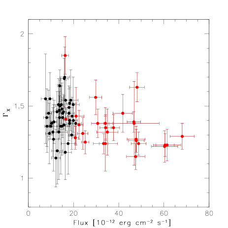
Figure 4: Swift/XRT photon index as a function of the 0.3–10 keV unabsorbed flux. The red points highlight the high-activity period.

During the Swift pointings, the UVOT instrument observed CTA 102 in all its optical ($v$, $b$, and $u$) and UV ($w1$, $m2$, and $w2$) photometric bands (Poole et al., 2008; Breeveld et al., 2010). We analysed the data using the uvotsource task included in the HEAsoft package (v6.22). Source counts were extracted from a circular region of five-arcsec radius centred on the source, while background counts were derived from a circular region of 20 arcsec radius in a nearby source-free region. Observed magnitudes are reported in Table 2. An increase of 4.5–5.5 mag with respect to the faint state of the source was observed in the UVOT bands, with a range of values: $v=11.44$–16.86, $b=12.56$–17.24, $u=11.78$–16.27, $w1=11.33$–16.18, $m2=11.36$–16.17, $w2=11.52$–16.46.

Following Raiteri et al. (2010, 2011), to obtain de-absorbed flux densities we used the count rate to flux density conversion factors $\rm CF$ and amount of Galactic extinction $A_{\Lambda}$ for each UVOT band that have been obtained by folding the quantities of interest with the source spectrum and effective areas of UVOT filters and are reported in Larionov et al. (2016).

Besides correcting flux densities for Galactic extinction, we also subtracted the thermal emission contribution due to the accretion disc and BLR according to the model by Raiteri et al. (2014).

4 Optical-to-radio observations

CTA 102 has been monitored by the GLAST-AGILE Support Program (GASP) of the WEBT in the optical, near-infrared and radio bands since 2008. Optical-to-radio GASP-WEBT data collected in 2013–2017 have been presented in Raiteri et al. (2017). That data set is here complemented with data at 15 GHz by the OVRO telescope, at 91 and 103 GHz by ALMA, in the near-IR by the REM telescope, in the optical by the Swift satellite. The optical photometric observations used in this paper were acquired at the following observatories: Abastumani (Georgia), AstroCamp (Spain), Belogradchik (Bulgaria), Calar Alto (Spain), Campo Imperatore (Italy), Crimean (Russia), Kitt Peak (USA), Lowell (USA; 70 cm, DCT and Perkins telescopes), Lulin (Taiwan), Michael Adrian (Germany), Mt. Maidanak (Uzbekistan), New Mexico Skies (USA), Osaka Kyoiku (Japan), Polakis (USA), Roque de los Muchachos (Spain; Liverpool, NOT and TNG telescopes), ROVOR (USA), Rozhen (Bulgaria; 200 and 50/70 cm telescopes), San Pedro Martir (Mexico), Sirio (Italy), Skinakas (Greece), Steward (USA; Kuiper, Bok, and Super-LOTIS), St. Petersburg (Russia), Teide (Spain), Tien Shan (Kazakhstan), Tijarafe (Spain), Tucson (USA), Valle d’Aosta (Italy), and Vidojevica (Serbia).

Near-IR data were collected within the WEBT project in the $J$, $H$, and $K$ bands at the Campo Imperatore, Lowell (Perkins) and Teide observatories. These data are here complemented with observations performed by REM (Zerbi et al., 2001; Covino et al., 2004), a robotic telescope located at the ESO Cerro La Silla observatory (Chile), in the period 2016 November 15–December 11. All raw near-IR frames obtained with the REM telescope were reduced following standard procedures. Instrumental magnitudes were obtained via aperture photometry and absolute calibration has been performed by means of secondary standard stars in the field reported by 2MASS. The data presented here were obtained as Target of Opportunity observations triggered by the $\gamma$-ray flaring activity of the source (PI: F. D’Ammando). Observed magnitudes are reported in in Table 3.

Optical and near-IR flux densities were dereddened following the prescriptions of the NASA/IPAC Extragalactic Database (NED) and corrected for the thermal emission contribution according to the model of Raiteri et al. (2017).

Radio and mm observations were done at the Metsähovi Radio Observatory (Finland) at 37 GHz, and at the 30-m IRAM telescope (Spain) and the Sub-millimeter Array (Hawaii, USA) at 230 GHz. We also added the ALMA data collected at 91 and 103 GHz (Band 3) during 2013–2017 and included in the ALMA calibrator source catalogue.

As part of an ongoing blazar monitoring program, the OVRO 40-Meter Telescope has observed CTA 102 at 15 GHz regularly since the beginning of 2009. The OVRO 40-Meter Telescope uses off-axis dual-beam optics and a cryogenic receiver with 2 GHz equivalent noise bandwidth centred at 15 GHz. Atmospheric and ground contributions as well as gain fluctuations are removed with the double switching technique (Readhead et al., 1989) where the observations are conducted in an ON–ON fashion so that one of the beams is always pointed on the source. Until 2014 May the two beams were rapidly alternated using a Dicke switch. Since 2014 May, when a new pseudo-correlation receiver replaced the old receiver, a 180 deg phase switch is used. Relative calibration is obtained with a temperature-stable noise diode to compensate for gain drifts. The primary flux density calibrator is 3C 286, with an assumed value of 3.44 Jy (Baars et al., 1977); DR21 is used as secondary calibrator source. Details of the observation and data reduction schemes are given in Richards et al. (2011). Observations acquired at 15 GHz by OVRO were used in this paper together with those obtained within the WEBT project. The radio flux at 15 GHz varied between 2.85 and 3.88 Jy during 2013–2017.

Radio-to-optical light curves collected by WEBT, REM, ALMA, and OVRO will be compared to the $\gamma$-ray light curve obtained by Fermi-LAT in the Section 5.

5 Multifrequency flux variability

Table 1: Variability amplitude estimated over the period 2013 January 1–2017 February 9 in the different energy bands. Values are corrected for Galactic extinction and the thermal emission contribution. For the minimum and maximum flux density the MJD at which the value is collected is reported in parenthesis.

Band	Minimum Flux density	Maximum Flux density	Variability amplitude
	(erg cm-2 s-1)	(erg cm-2 s-1)
$\gamma$ rays	5.91$\times$10-13 (MJD 57177–57181)	3.02$\times$10-9 (MJD 57752–57756)	5110
X-ray	7.60$\times$10-12 (MJD 57386)	6.81$\times$10-11 (MJD 57759)	9
W2	1.95$\times$10-12 (MJD 56958)	4.92$\times$10-10 (MJD 57751)	253
M2	3.41$\times$10-12 (MJD 56958)	6.90$\times$10-10 (MJD 57752)	202
W1	2.55$\times$10-12 (MJD 56958)	5.95$\times$10-10 (MJD 57751)	233
U	2.50$\times$10-12 (MJD 56958)	3.37$\times$10-10 (MJD 57752)	135
B	2.98$\times$10-13 (MJD 56893)	7.20$\times$10-10 (MJD 57750)	2416
V	1.97$\times$10-13 (MJD 56874)	7.71$\times$10-10 (MJD 57750)	3920
R	2.20$\times$10-13 (MJD 56785)	7.76$\times$10-10 (MJD 57750)	3523
I	3.62$\times$10-13 (MJD 56785)	8.01$\times$10-10 (MJD 57750)	2210
J	6.18$\times$10-13 (MJD 56879)	6.96$\times$10-10 (MJD 57752)	1126
H	8.59$\times$10-13 (MJD 56879)	7.10$\times$10-10 (MJD 57752)	827
K	1.09$\times$10-12 (MJD 56879)	5.73$\times$10-10 (MJD 57751)	526
230 GHz	2.25$\times$10-12 (MJD 56832)	1.62$\times$10-11 (MJD 57754)	7
103 GHz	1.63$\times$10-12 (MJD 56837)	6.93$\times$10-12 (MJD 57649)	4.3
91 GHz	1.51$\times$10-12 (MJD 56837)	5.84$\times$10-12 (MJD 57649)	3.9
37 GHz	7.92$\times$10-13 (MJD 56839)	1.89$\times$10-12 (MJD 57671)	2
15 GHz	4.28$\times$10-13 (MJD 56651)	5.99$\times$10-13 (MJD 57708)	1.5

Variability studies of radio-to-$\gamma$-ray emission from blazars can provide important insights into the physics of the jet and the mechanisms at work in these sources. Flares can be explained e.g. by a shock propagating downstream the jet and/or by variations of the Doppler factor, which depends on the bulk Lorentz factor of the relativistic plasma in the jet and on the viewing angle. During flares, blazars usually show greater variability amplitudes in the high-energy part of the spectrum than in the low-energy one (e.g., Wehrle et al., 1998; Raiteri et al., 2012). However, some sources increased their brightness by hundreds of times also in infrared and optical bands. In this context, the 2016–2017 outburst of CTA 102 presented here is one of the best cases to study.

We quantify the observed variability of the CTA 102 jet emission in the different energy bands through the variability amplitude, calculated as the ratio of maximum to minimum flux. Values in the $\gamma$-ray band are based on the light curve with five-day time bins. Near-infrared-to-UV fluxes are corrected for Galactic extinction. Moreover, the contribution of the thermal emission from the disc, BLR, and torus is removed to properly consider only the jet contribution to the flux. In Table 1 and Fig. 5, we report the variability amplitude estimated over the period 2013 January 1–2017 February 9 in the different bands. The variability amplitude may depend on the sampling of the light curves at the different frequencies. In the case of CTA 102, observations were available in all energy bands at the peak of the flare, making the values obtained representative of the increase of activity of the source. The variability amplitude shows a rising trend with increasing frequency in the radio-to-optical range and it declines in the UV. The X-ray band has a small variability amplitude, in particular if compared to the $\gamma$-ray one. This can be related to the lower energies of the electrons producing X-rays with respect to those producing $\gamma$ rays. The similar variability amplitude at 230 GHz and in the X rays may be a hint that they are produced by the same electron population in the same jet region through the synchrotron and IC emission mechanism, respectively, as found e.g. for BL Lacertae (Raiteri et al., 2013).

Figure 5: Variability amplitude vs frequency in the different energy bands estimated over the period 2013 January 1–-2017 February 9. Values are corrected for Galactic extinction and the thermal emission contribution.

Figure 6: Multifrequency light curve normalized to the maximum value observed for the period 2016 November 11–2017 February 8 (MJD 57003–57792) in the following energy bands (from top to bottom): $\gamma$ rays (100 MeV–300 GeV), X-rays (0.3–10 keV), $B$, $V$, $R$, $I$, $J$, $H$, and $K$. Filled triangles: WEBT data; open triangles: UVOT data; open squares: REM data. Main $\gamma$-ray outbursts are labelled as F1, F2, F3, and F4 in the top panel.

Simultaneous flux variations at low and high energies indicate that their emission comes from the same region of the jet and that the same electrons produce both the synchrotron and IC fluxes (e.g., Fossati et al., 2008). However, flaring events in the optical band with no counterpart at high energies were observed in some blazars (e.g., Chatterjee et al., 2013; D’Ammando et al., 2013). Strong variability characterizes the emission over the entire electromagnetic spectrum of CTA 102 in 2016–2017, in particular during the period 2016 November 11–2017 February 8 (MJD 57003–57792), making this an ideal target to investigate the connection of the flux behaviour observed in $\gamma$ rays with the flux behaviour at lower energies.

In Fig. 6, we compare the $\gamma$-ray light curve obtained by Fermi-LAT with 12-h time bins during the highest activity period, 2016 November 11–2017 February 8 (MJD 57003–57792, corresponding to the outburst VI in Fig. 2), to the infrared-to-X-ray light curves. All fluxes are normalized to the maximum value observed in the considered period in order to compare when and how much the flux increased in the different energy bands. In the $\gamma$-ray light curve we can see four major outbursts peaked on 2016 December 15 (MJD 57737; F1), 2016 December 22 (MJD 57744; F2), 2016 December 27 (MJD 57749; F3), and 2017 January 4 (MJD 57757; F4). The third outburst appears more prominent and shows a larger increase with respect to the others. These four outbursts have corresponding events in optical, with the peaks observed at the same time. In $J$, $H$, and $K$ bands the sampling is sparse and only two of the four peaks are observed. A high X-ray flux has been observed in the period that covers the $\gamma$-ray flares F1 and F2, and two X-ray peaks are evident at the time of the $\gamma$-ray flares F3 and F4.

If we compare the $\gamma$-ray and optical ($R$ band, the best sampled band) fluxes normalized to the respective lowest values observed during 2016 November 11–2017 February 9 (Fig. 7), it is evident that the four main flares occurred at the same time. A similar amplitude has been observed in the two bands, except for the first flare. In particular, the same variability amplitude has been observed during the main peak. On the other hand, not all the events observed in the optical band have a counterpart in $\gamma$ rays and vice versa. In addition to the “sterile” optical flare occurred around 2016 December 1 (MJD 57723), no significant optical activity corresponds to the increase of $\gamma$-ray activity peaked on 2017 January 24 (MJD 57777) and 2017 February 6 (MJD 57790) (“orphan” flares). This indicates that the interpretation of the source variability must be more complicated than the fair overall optical-$\gamma$ correlation would suggest.

Cross-correlation analysis between flux variations in different bands can allow us to determine whether the emissions come from the same region of the jet or not. We used the discrete correlation function (DCF; Edelson & Krolik, 1988; Hufnagel & Bregman, 1992) to analyze cross-correlations. Correlation produces positive peaks in the DCF and is strong if the peak value approaches or even exceeds one. The DCF between the $\gamma$-ray and the optical ($R$-band) light curves over the whole 2013–2017 period is displayed in Fig. 8, showing a main peak compatible with no time lag. When comparing the $\gamma$-ray light curve with 12-h time bin with the optical light curve with one-hour binning in the high-activity period of Fig. 7, the DCF shows again a main peak compatible with no time lag, with DCF_p = 0.94 (Fig. 9). This indicates strong correlation between $\gamma$-ray and optical emission, with no evidence of delay between the flux variations in the two bands, in agreement with the results presented in Larionov et al. (2017). We determine the uncertainty in this result by performing 1000 Monte Carlo simulations according to the “flux redistribution/random subset selection” technique (Peterson et al., 1998; Raiteri et al., 2003), which tests the importance of sampling and data errors. Among the 1000 simulations, we obtain that 78.3 per cent of simulations ($>1$ $\sigma$) give a time lag between 0 and 0.6 d, as shown in the inset of Fig. 9. This is compatible with no delay between optical and $\gamma$-ray emission. The secondary DCF peaks in Fig. 9 are due to the multi-peaked structure of the outburst.

Figure 7: Comparison of the Fermi-LAT $\gamma$-ray light curve with 12-h time bins (top panel) and $R$-band light curve (bottom panel) normalized to the lowest value observed in the period 2016 November 11–2017 February 8. Main $\gamma$-ray outbursts and “orphan” flares are labelled as F1, F2, F3, F4, and orphan in the top panel. The “sterile” flare is labelled as sterile in the bottom panel.

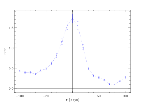
Figure 8: DCF between the $\gamma$-ray fluxes obtained with five-day time bins and the $R$-band flux densities with 1 day binning over the whole 2013–2017 period.

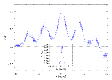
Figure 9: DCF between the $\gamma$-ray fluxes obtained with 12-h time bins and the $R$-band flux densities with one-hour binning during the 2016–2017 flaring period. The inset shows the result of cross-correlating 1000 Monte Carlo realizations of the two data sets according to the “flux redistribution/random subset selection” technique.

Although the UV data collected by Swift-UVOT are sparser than the optical ones, we can recognize a similar behaviour in the $\gamma$-ray and UV light curves with similar increase of flux during the flaring period when normalized to the maximum value (Fig. 10), even though the variability amplitude is smaller in UV with respect to the $\gamma$-ray band.

The sparse X-ray data in 2013–2015 indicate a low flux, in keeping with the relatively low activity observed also in $\gamma$ rays (see Fig. 2). The comparison between the $\gamma$-ray and the X-ray light curves during the high-activity period shows a general agreement, with the $\gamma$-ray peaks corresponding to high X-ray fluxes (Fig. 11). Cross-correlation of the $\gamma$-ray (12-h time bins) and X-ray light curves in the high-activity period shows a good correlation with a time lag compatible to zero within the DCF bin size of six days (Fig. 12). The different sampling of the light curves does not allow a more detailed comparison. However, the X-ray variability amplitude appears much smaller than at $\gamma$ rays.

Figure 10: Multifrequency light curve normalized to the maximum value observed for the period 2016 November 11–2017 February 8 (MJD 57003–57792) in the following energy bands (from top to bottom): $\gamma$ rays (100 MeV–300 GeV), $w2$, $m2$, and $w1$ bands.

Figure 11: Fermi-LAT $\gamma$-ray light curve with 12-h time bins in the 0.1–300 GeV energy range (top panel) and X-ray light curve in the 0.3–10 keV energy range (bottom panel) in the period 2016 November 11–2017 February 9.

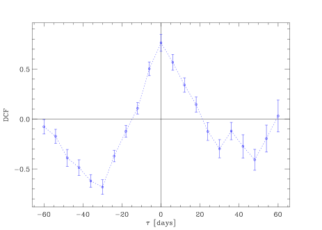
Figure 12: DCF between the $\gamma$-ray fluxes obtained with 12-h time bins and the X-ray flux.

The correlation between the radio-mm fluxes on one side and the optical and $\gamma$-ray fluxes on the other side is rather puzzling. In general, they present a different behavior, but sometimes they share common features. As one can see in Fig. 13, the mm data at 230 GHz show a steady flux increase starting from the end of 2015 and culminating with a prominent outburst peaking on 2017 January 1 (MJD 57754). A comparison with the $\gamma$-ray light curve reveals that the end of 2015 also marks the beginning of the activity in this band, with the major peak observed at the same time of the 230 GHz one.

A steady flux increase starting from the end of 2015 is observed also at 91–103 GHz, is marginally detectable at 37 GHz, and vanishes at 15 GHz. Enhanced activity is present at the beginning of 2014 at 230, 91–103, and 37 GHz, when the light curves at both lower and higher frequencies appear rather flat.

The light curves at 91–103, 37, and 15 GHz present peaks in 2016 October–November. The increase of delay of the radio peaks going to lower frequencies is in agreement with synchrotron self-absorption opacity effects. The decrease of the flux variation amplitudes towards lower frequencies is expected, if the radio emission at lower frequencies comes from more external and extended regions of the jet, in average less aligned to our line of sight. In and around the same period, the sampling at 230 GHz is poor. The closest events at $\gamma$-ray and optical frequencies date 2016 August (flare V in Fig. 2), and, before, there is a stronger $\gamma$-ray flare in 2016 March (flare IV) during a seasonal gap in the optical light curve.

The DCF between the $\gamma$-ray and 15 GHz fluxes (see Fig. 14) shows a small peak at a negative time lag of about two months, indicating radio variations preceding the $\gamma$-ray ones. This signal comes from the cross-match of the 15 GHz flare peaking at the beginning of 2016 November with the $\gamma$-ray acme two months later. A stronger DCF maximum occurs at time lag of about 250 d, indicating radio variations following the $\gamma$-ray ones by about eight to nine months. This suggests that linking the 2016 October–November radio flare observed from 103 to 15 GHz with the 2016 March $\gamma$-ray flare is more likely. Therefore, a delayed radio outburst at 15 GHz can be expected also some months after the 2017 January main flare observed in the $\gamma$-ray, optical, and 230 GHz band.

However, extending the OVRO light curve at 15 GHz up to 2018 July (see Fig. 18), a radio outburst is visible only in 2018 February, more than one year after the 2017 $\gamma$-ray, optical and mm peaks. Its peak flux is only a few percent greater than the maximum flux reached in 2016 October–November. On the basis of the delay between $\gamma$-ray emission and radio emission at 15 GHz found here and usually observed in blazar objects (e.g., Pushkarev et al., 2010; Fuhrmann et al., 2014), it is unlikely that the 2018 radio outburst at 15 GHz is related to the main flaring activity observed at the beginning of 2017 in $\gamma$-ray, optical, and at 230 GHz. Therefore, we conclude that the $\gamma$-ray flaring activity in 2017 has no (delayed) counterpart in the 15 GHz light curve.

Figure 13: Multifrequency light curve for the period 2013 January 1–2017 February 9 in the following energy bands (from top to bottom): $\gamma$ rays (100 MeV–300 GeV; 5-d time bins, in units of 10^-8 ph cm^-2 s^-1; Fermi-LAT data), 230 GHz (in units of Jy; triangles: SMA data, squares: IRAM data), 91 and 103 GHz (in units of Jy; ALMA data), 37 GHz (in units of Jy; Metsähovi data), 15 GHz (in units of Jy; OVRO data).

In the framework of the geometrical model, the difference in behaviour between radio and higher energy emission would be ascribed to different viewing angle (with consequent different Doppler boosting of the emission) of the jet regions producing their emission. The extent of misalignment between the emitting jet regions can be inferred from the corresponding light curves, as will be shown in Sect. 7.

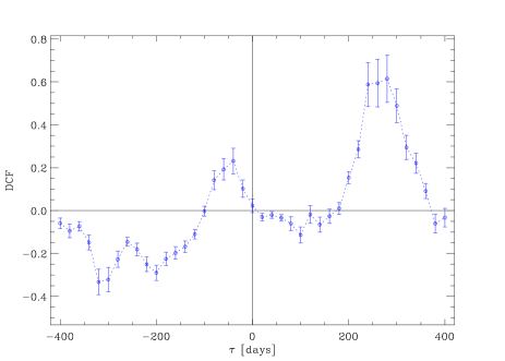
Figure 14: DCF between the $\gamma$-ray fluxes obtained with five-day time bins and the 15 GHz flux densities.

6 Multifrequency spectral variability

Figure 15 shows the broad-band SED of CTA 102 in three brightness states with near-contemporaneous data in the optical, UV, X-ray, and $\gamma$-ray bands. The optical-to-radio data set presented in Raiteri et al. (2017) has been complemented with data at 15 GHz by the OVRO telescope, at 91 and 103 GHz by ALMA, and in the near-IR by the REM telescope, in the optical-to-X-rays by the Swift satellite, and at $\gamma$ rays by the Fermi satellite. In addition to SMA, Metsähovi, ALMA, and OVRO data, radio observations collected by RATAN-600 radio telescope (Mingaliev et al., 2001) from 1.0 to 21.7 GHz have been considered. Because of the longer variability time-scales of the radio light curves, radio data are included also if taken within a few days from the reference epoch.

The highest state corresponds to $\rm MJD=57761$ (2017 January 8). Optical data were acquired at the Tijarafe Observatory and fairly overlap with the UVOT data. The intermediate state dates $\rm MJD=57635$ (2016 September 4), and comes from the declining phase of the small flare preceding the big outburst (flare V in Fig. 2). The optical data are from the Mt.  Maidanak Observatory and are in satisfactorily agreement with the UVOT data. For the low state, we chose $\rm MJD=57364$ (2015 December 8), about one year before the culmination of the big outburst. Optical data are from the St. Petersburg Observatory; the $B$-band point appears a bit fainter than the corresponding UVOT value, but they agree within errors. For the LAT data the spectra are extracted on 5-day time-scale as done in Fig. 2, except for the high state in which the daily LAT spectrum is included.

The intermediate- and the low-state SED become very close in the UV, where the emission contribution of the big blue bump peaks in coincidence of the Ly$\alpha\lambda$1216 broad emission lines. The X-ray spectral shape in the intermediate state is softer than expected, but it is affected by large errors. Finally, the peak of the IC component shifts at a much higher energy in the high state, confirming the result found for the synchrotron component by Raiteri et al. (2017).

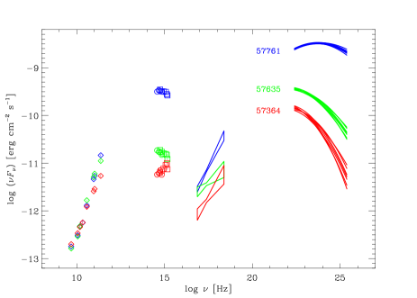
Figure 15: Broad-band SED of CTA 102 in three different brightness states labelled with their MJD. In the optical-UV bands, ground-based data are shown as open circles, while UVOT data are displayed with squares. The X-ray spectra are represented by PL fits, while the Fermi-LAT spectra are plotted according to LP models; in both cases we took the uncertainties on the parameters into account.

7 Geometrical model applied to $\gamma$-ray, optical, and radio data

In Raiteri et al. (2017) we interpreted the long-term variability of the CTA 102 synchrotron flux in terms of variation of the Doppler factor because of changes of the viewing angle of the jet-emitting regions. The intrinsic flux is assumed to be constant on time-scales of months or longer in the rest frame, while flast flares can be due to intrinsic, energetic processes. From the observed multiwavelength light curves we derived how the jet moves, i.e. how the regions emitting at different frequencies align with respect to the line of sight. Support to this twisting jet scenario comes from both observations and theory. Examples of helical jet structures and wobbling motion have been observed with high angular resolution images in the radio band in both extragalactic and Galactic sources (see e.g., Agudo et al., 2007, 2012; Perucho et al., 2012; Fromm et al., 2013; Britzen et al., 2017, 2018; Miller-Jones et al., 2019).

In numerical magnetohydrodynamics (MHD) simulations of relativistic jets in 3D, instabilities can develop which distort the jet itself and produce wiggled structures (Nakamura et al., 2001; Mignone et al., 2010). Moreover, orbital motion in a binary black hole system or a warped accretion disc can lead to jet precession, which modifies the jet orientation with respect to the line of sight (Liska et al., 2018).

Raiteri et al. (2017) performed their analysis on radio–optical data, concentrating on the light curves at 37 and 230 GHz, and in the $R$ band. In the following we investigate the outcome of the proposed geometrical model when applied to both higher and lower frequencies. We examine the $\gamma$-ray and 15 GHz flux variability; the X-ray data are too sparse for a meaningful analysis. We consider the $\gamma$-ray light curve from 2013 January 1 (MJD 56293), with a time bin of five days before 2016 November 11 (MJD 57703) and 12 h after. The $\gamma$-ray light curve is compared to the optical ($R$ band) and radio (15 GHz) light curves in Fig. 16.

As in Raiteri et al. (2017), we modelled the optical long-term trend with a cubic spline interpolation through the data binned with a variable time interval, which shortens as the flux rises: $\Delta t=\Delta t_{0}/n$ when $F>F_{\rm min}n^{2+\alpha}$, where the exponent 2 applies to a continuous jet and $\alpha=1.7$ is the spectral index in the $R$ band. We used the same binning to obtain the spline in the $\gamma$-ray band, while for 15 GHz case we adopted a 30-d bin because of the smoother behaviour, as done by Raiteri et al. (2017) for the 37 and 230 GHz light curves.

From the splines we derived the Doppler factors $\delta(t)$ displayed in Fig. 16 as

$$\delta(t)=\delta_{\rm min}\,(F_{\rm spline}/F_{\rm min})^{1/(2+\alpha)}$$

where $F_{\rm spline}$ are the flux densities defined by the spline interpolations, $F_{\rm min}$ are their minimum values, and $\delta_{\rm min}=3.7$ is obtained by assuming a bulk Lorentz factor $\Gamma=20$ and a maximum jet viewing angle $\theta_{\rm max}=9$ deg (Raiteri et al., 2017). We adopted a spectral index equal to the optical one for the $\gamma$-ray band and equal to zero for the 15 GHz case.

The behaviour of $\delta(t)$ in the optical and $\gamma$-ray bands are in fair general agreement, as expected if the optical and $\gamma$-ray photons are produced in the same jet region. Small differences between the Doppler factor estimated in the optical and $\gamma$-ray bands are justified by the fact that we derived the Doppler factors by interpolating through data affected by errors and collected in bands with different samplings. There is some discordance only in the last part of the considered period, where some $\gamma$-ray activity has no optical counterpart (see discussion in the next section).

In contrast with the optical and $\gamma$-ray cases, the Doppler factor resulting from the 15 GHz long-term trend is only marginally variable. Actually, in general the Doppler factor and its variability decrease from 230 to 15 GHz, in agreement with the decrease of their flux variability amplitude.

We interpret the time variability of the Doppler factor as due to changes in the jet viewing angle, which implies a twisting jet. The trend of the viewing angle is derived from the definition of the Doppler factor and is shown in Fig. 16. The flux maxima correspond to maxima in the Doppler factor and minima in the viewing angle. The plots of $\theta(t)$ suggest that the part of the jet producing the optical and $\gamma$-ray radiation is characterized by intense wiggling, the viewing angle ranging from about nine to two degrees. In contrast, the viewing angle remains more stable as we proceed towards longer wavelengths, i.e. towards outer and larger jet regions. At 15 GHz $\theta(t)$ varies between 8.4 and 9 degrees. Indeed, the viewing angle of the radio-emitting regions can be seen as an average over extended zones of the curved jet. This would also be the reason why the rise of the 230 GHz flux towards the 2016–2017 peak starts much earlier than in the optical and $\gamma$-ray bands. Indeed, while the optical and $\gamma$-ray fluxes reach the minimum viewing angle abruptly, the larger and curved jet section emitting the millimetre flux starts to align with the line of sight even before the optical and $\gamma$-ray-emitting zone. The maximum “misalignment” between the $\gamma$-optical and 15 GHz emitting regions is reached during the culmination of the 2016–2017 outburst and is about seven degrees.

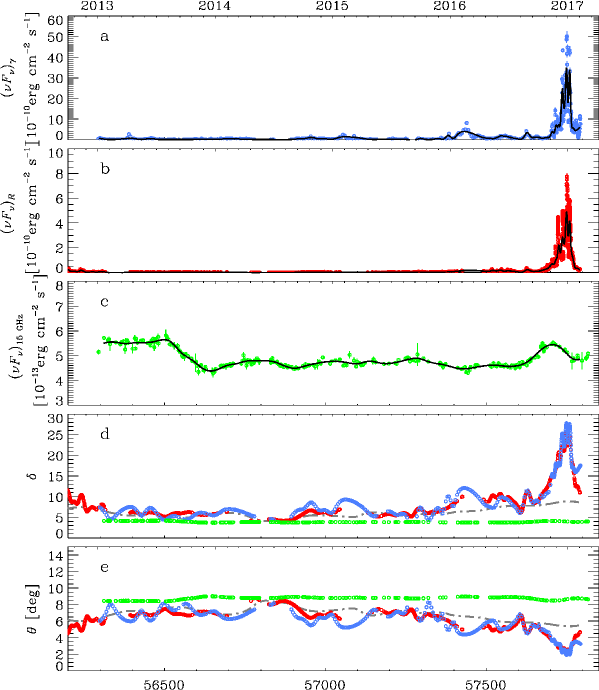
Figure 16: Light curves of CTA 102 in the $\gamma$-ray (a), optical (b), and 15 GHz radio (c) bands. The black curves indicate splines interpolations with variable time bin in the optical and $\gamma$-ray bands, and 30-d bins at 15 GHz; they represent the long-term trends. The Doppler factor $\delta$ for the $\gamma$-ray (blue), the optical (red), and the radio (green) bands are plotted in panel (d), while (e) shows the corresponding viewing angles. In panel (d) and (e) the grey dot–dashed curve shows the trend obtained for the 230 GHz data according to Raiteri et al. (2017).

In Fig. 17 we show the relationship between $\gamma$-ray and optical fluxes starting from 2013 January 1 (MJD 56293). Each $\gamma$-ray flux is associated with the average of the optical fluxes acquired within 2.5 d from the time of the $\gamma$ data point when the $\gamma$-ray bin is five days, within six hours when the bin is 12 h. The slope of the linear fit is 0.82 and the linear Pearson correlation coefficient is 0.95.

The geometrical effect is expected to be more evident during the outburst, when we also have better sampling. If we restrict the linear fit to the outburst data in the time interval 2016 November 23–2017 January 22 (MJD 57715–57775), we obtain a linear fit with slope equal to 1.00 and linear Pearson correlation coefficient equal to 0.90. A unity slope is what one expects if both the $\gamma$-ray and optical long-term trends are due to Doppler factor variations (Larionov et al., 2016), so this result supports the idea that the variability during the outburst is mainly caused by changes in $\delta$, as predicted by the geometrical model.

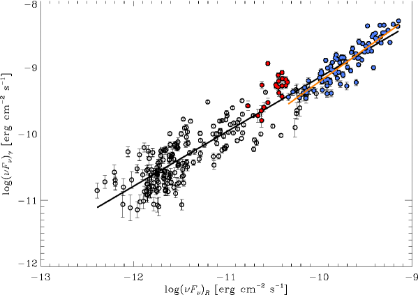
Figure 17: The relationship between $\gamma$-ray and optical fluxes. The $\gamma$-ray fluxes have been associated with the average optical fluxes obtained by considering optical data close in time to the $\gamma$-ray optical points. The blue dots refer to the outburst period, the red dots to the period of the $\gamma$-ray “orphan” flare ($\rm MJD>57775$). The black and orange solid lines represent linear fits to all the data and to the data in the outbust period, respectively.

8 Discussion and conclusions

In Raiteri et al. (2017) the results of radio-to-optical monitoring of the FSRQ CTA 102 in 2013–2017 were presented and a geometrical model was applied to those data. In this paper, that data set has been complemented with data at 15 GHz by the OVRO telescope, at 91 and 103 GHz by ALMA, in the near-IR by the REM telescope, in the optical-to-X-rays by the Swift satellite, and at $\gamma$ rays by the Fermi satellite. These new data have been analysed in view of the above geometrical interpretation.

Since 2013 April, the source showed significant flux and spectral variability in $\gamma$ rays on a monthly time-scale, with several periods of high activity. A general correlation is found between the optical, infrared, and $\gamma$-ray flux variations, which are consistent with being simultaneous, suggesting that the observed emission is produced in the same region of the jet.

The source showed strong activity in the period mid 2016–February 2017 at all frequencies. In particular, an unprecedented $\gamma$-ray flaring activity was observed, reaching a peak flux of (2158 $\pm$ 63) $\times$10^-8 ph cm^-2 s^-1 in the 0.1–300 GeV energy range on 2016 December 28, corresponding to an apparent isotropic luminosity of (2.2 $\pm$ 0.1)$\times$10⁵⁰ erg s^-1. Comparable values are obtained on 12-h time bin in the same day. The peak luminosity observed for CTA 102 is comparable to the highest values observed in blazars so far. Four main outbursts are observed in $\gamma$ rays between 2016 November 11 and 2017 February 9, and corresponding events are observed in near-IR, optical, and UV with the peaks at the same time. A common trend was observed also between the X-ray and $\gamma$-ray emission in the high activity state. No significant harder-when-brighter behaviour was observed in X-rays, indicating that a change in the electron energy distribution is not the main driver of the variability in this band.

The same variability amplitude was observed in the optical ($R$ band) and $\gamma$ ray bands during the high-activity period. DCF analysis suggests a strong correlation between the flux variations in optical and $\gamma$ rays, with no detectable lag between the emission in the two bands. However, not all the events observed in the optical band have a counterpart in $\gamma$ rays and vice versa. The interpretation of these “orphan flares” is a challenge for all theoretical models aiming to explain blazar variability. They are likely produced in a different emitting region or by a different emission process (e.g., magnetic reconnection; Petropoulou et al., 2016) with respect to the emitting region and mechanism responsible for the long-term behaviour.

On the other hand, the “sterile” optical flare observed around 2016 December 1 (MJD 57723) can be due to the fact that the optical emitting region presents substructures (e.g., Narayan & Piran, 2012), and not all of them produce significant $\gamma$-ray emission. Alternatively, magnitude and direction of a turbulent magnetic field should affect mostly the synchrotron emission, producing an increase of flux in optical not observed in $\gamma$ rays (e.g., Marscher et al., 2014). These “sterile” and “orphan” flares are superposed to the long-term variability well explained by the geometrical model adopted here.

We have investigated the source behaviour at higher ($\gamma$-ray) and lower (15 GHz) frequencies than those analysed in Raiteri et al. (2017) by means of their geometrical interpretation of the source variability. This model implies that different emitting regions can change their alignment with respect to the line of sight, leading to a different Doppler boosting and thus enhancement of the observed flux from one region with respect to that from another region. We have derived the trends in time of the Doppler factor and of the viewing angle for the jet regions responsible for the $\gamma$-ray and 15 GHz emission. The trends inferred from the $\gamma$-ray data are in fair agreement with the optical ones and the relationship between the $\gamma$-ray and optical fluxes is linear, as predicted by the model, confirming it. We note that a $\gamma$-ray/optical linear correlation during the outburst may be obtained also with a change of the electron density within a leptonic, one-zone model, where the $\gamma$ rays are produced by an external Compton mechanism. However, the geometrical model also accounts for the continuous time evolution of the multiwavelength flux and not only for single snap-shots of the source behaviour.

A change in the direction of the jet, which became oriented more closely to our line of sight ($\theta$ $\sim$ 1.2 deg), has been observed with Very Long Baseline Array images at 43 GHz during the $\gamma$-ray flaring activity of CTA 102 in 2012 September–October (Casadio et al., 2015). These orientation changes can be due to MHD instabilities developing in the jet, precession, or orbital motions in a binary system of supermassive black holes.

Alternative theoretical scenarios have been proposed to explain the flaring activity observed during 2016–2017 in CTA 102. In particular, the multiwavelength flares from 2016 December to 2017 January are explained by Casadio et al. (2019) as the interaction between a new jet component and a possible recollimation shock at $\sim$0.1 mas. The variability Doppler factor associated with such interaction (i.e. $\delta_{\rm\,var}$ = 34 $\pm$ 4) is compatible with the values obtained applying our geometrical model (see Fig. 16). However, Casadio et al. (2019) did not try to reproduce the evolution in time of the flaring activity or the long-term behaviour of the multi-wavelength light curves with their model.

The long-term trend in optical, X-ray, and $\gamma$-ray band has been discussed in a scenario in which the increase of activity is due to the ablation of a gas cloud by the relativistic jet within a hadronic emission model in Zacharias et al. (2019). However, the proposed hadronic model results in super-Eddington jet powers at all times. This is a common problem in the application of hadronic models to the SED modelling of blazars (e.g., Böttcher et al., 2013). These extreme jet powers obtained in hadronic models are in conflict with the estimates of the jet power based on radio lobes and X-ray cavities (e.g., Merloni et al., 2007; Godfrey & Shabala, 2013), and the corresponding accretion rates should imply a very short accretion mode and/or a very small duty cycle in the SMBH evolution compared to estimated lifetimes of active phases of AGN (e.g., Zdziarski & Boettcher, 2015). Moreover, the optical and X-ray coverage, both in the flaring and long-term periods, at which the theoretical model proposed in Zacharias et al. (2019) has been applied appears not adequate to obtain robust results due to long gaps of data and relatively small number of data. The details of the model should be tested with more complete data set like that presented in this paper.

We conclude that the observed long-term flux and spectral variability of CTA 102 at both low and high energies can well be explained by an inhomogeneous curved jet where the observed emission at different frequencies is modulated by changes in the orientation of the corresponding emitting regions with respect to our line of sight.

The main strength of this geometrical model is that it can explain the long-term flux and spectral evolution of CTA 102 in a simple way, with very few assumptions. Its main justification is its ability to explain the contraction of the variability time-scales and the increase of variability amplitude during outburst found by Raiteri et al. (2017). That is the signature of Doppler factor variations which cannot be justified by other models. The analysis performed in this paper, on a wider data set extending to high energies, confirms the model, showing in particular that the relationship between the $\gamma$-ray and optical fluxes is linear, as predicted by the model.

¹INAF - Istituto di Radioastronomia, Via Gobetti 101, I-40129 Bologna, Italy
²INAF - Osservatorio Astrofisico di Torino, Via P. Torinese, I- Torino, Italy
³Instituto de Astrofisica de Canarias (IAC), La Laguna, E-38200 Tenerife, Spain
⁴Departamento de Astrofisica, Universidad de La Laguna, La Laguna, E-38205 Tenerife, Spain
⁵Instituto de Astrofísica de Andalucía (CSIC), E-18080 Granada, Spain
⁶Pulkovo Observatory, 196140 St. Petersburg, Russia
⁷Institute of Astronomy and NAO, Bulgarian Academy of Sciences, 1784 Sofia, Bulgaria
⁸Crimean Astrophysical Observatory RAS, P/O Nauchny, 298409, Russia
⁹Instituto de Astronomía, Universidad Nacional Autónoma de México, 04510 Ciudad de México, México
¹⁰INAF, TNG Fundación Galileo Galilei, E-38712 La Palma, Spain
¹¹Department of Astronomy, Faculty of Physics, University of Sofia, BG-1164 Sofia, Bulgaria
¹²Osservatorio Astronomico della Regione Autonoma Valle d’Aosta, I-11020, Nus, Italy
¹³EPT Observatories, Tijarafe, E-38780 La Palma, Spain
¹⁴Max-Planck-Institut für Radioastronomie, D–53121, Bonn, Germany
¹⁵School of Physics & Astronomy, University of Southampton, Southampton, SO17 1BJ, UK
¹⁶Graduate Institute of Astronomy, National Central University, Jhongli City, Taoyuan County 32001, Taiwan
¹⁷Astronomical Observatory, 11060 Belgrade, Serbia
¹⁸INAF, Osservatorio Astronomico di Roma, I-00040 Monte Porzio Catone, Italy
¹⁹Ulugh Beg Astronomical Institute, Maidanak Observatory, Tashkent, 100052, Uzbekistan
²⁰Astronomical Institute, St. Petersburg State University, 198504 St. Petersburg, Russia
²¹Center for Astrophysics |  Harvard & Smithsonian, 60 Garden Street, Cambridge, MA 02138 USA
²²Astrophysics Research Institute, Liverpool John Moores University, Liverpool L3 5RF, UK
²³School of Cosmic Physics, Dublin Institute For Advanced Studies, Ireland
²⁴Institute for Astrophysical Research, Boston University, Boston, MA 02215, USA
²⁵NNLOT, Al-Farabi Kazakh National University, 050040 Almaty, Kazakhstan
²⁶Fesenkov Astrophysical Institute, Almaty, Kazakhstan
²⁷Abastumani Observatory, Mt. Kanobili, 0301 Abastumani, Georgia
²⁸Engelhardt Astronomical Observatory, Kazan Federal University, 422526 Tatarstan, Russia
²⁹Landessternwarte, Zentrum für Astronomie der Universität Heidelberg, 69117 Heidelberg, Germany
³⁰Center for Astrophysics, Guangzhou University, Guangzhou, 510006, China
³¹Aalto University Metsähovi Radio Observatory, FI-02540 Kylmälä, Finland
³²Aalto University Dept of Electronics and Nanoengineering, FI-00076 Aalto, Finland
³³Astronomical Institute, Osaka Kyoiku University, Osaka, 582-8582, Japan
³⁴UCD School of Physics, University College Dublin, Dublin 4, Ireland
³⁵Department of Physics and Astronomy, Brigham Young University, Provo, UT 84602, USA
³⁶Michael Adrian Observatorium, Astronomie Stiftung Trebur, 65468 Trebur, Germany
³⁷University of Applied Sciences, Technische Hochschule Mittelhessen, 61169 Friedberg, Germany
³⁸Command Module Observatory, 121 W. Alameda Dr., Tempe, AZ 85282, USA
³⁹Nordic Optical Telescope, E-38700 Santa Cruz de La Palma, Santa Cruz de Tenerife, Spain
⁴⁰Osservatorio Astronomico Sirio, I-70013 Castellana Grotte, Italy
⁴¹LESIA, Observatoire de Paris, Université PSL, CNRS, Sorbonne Université, Univ. Paris Diderot, Sorbonne Paris Cité, 5 place Jules Janssen, 92195 Meudon, France
⁴²Department of Physics, University of Colorado Denver, CO, 80217-3364 USA
⁴³Lowell Observatory, Flagstaff, AZ 85751, USA
⁴⁴Steward Observatory, University of Arizona, Tucson, AZ 85721, USA
⁴⁵Instituto de Radio Astronomía Milimétrica, E-18012 Granada, Spain
⁴⁶Finnish Center for Astronomy with ESO (FINCA), University of Turku, FI-20014, Turku, Finland
⁴⁷Aalto University Metsähovi Radio Observatory, Metsähovintie 114, 02540 Kylmälä, Finland
⁴⁸Owens Valley Radio Observatory, California Institute of Technology, Pasadena, CA 91125, USA
⁴⁹Departamento de Astronomía, Universidad de Chile, Camino El Observatorio 1515, Las Condes, Santiago, Chile
⁵⁰Departamento de Astronomia, Universidad de Concepcion, Concepcion, Chile
⁵¹Shanghai Astronomical Observatory, Chinese Academy of Sciences, Shanghai 200030, China
⁵²Kazan Federal University, 18 Kremlyovskaya St., Kazan 420044, Russia
⁵³Special Astrophysical Observatory of RAS, Nizhnij Arkhyz 369167, Russia

Appendix A Online Tables and Figures

Table 1: Log and fitting results of Swift-XRT observations of CTA 102 using a PL model with $N_{\rm H}$ fixed to Galactic absorption. Fluxes are corrected for the Galactic absorption.

Date (UT)	MJD	Net exposure time	Flux 0.3–10 keV	Photon index
		(s)	($\times$10-13 erg cm-2 s-1)	($\Gamma_{\rm\,X}$)
2013-May-24	56436	1041	$8.2\pm 1.4$	$1.42\pm 0.20$
2013-Jun-20	56463	3019	$11.2\pm 1.2$	$1.39\pm 0.12$
2013-Jun-23	56466	2974	$8.3\pm 1.1$	$1.36\pm 0.18$
2014-Oct-28	56958	4942	$10.3\pm 0.7$	$1.38\pm 0.08$
2014-Oct-30	56960	4942	$9.9\pm 0.7$	$1.36\pm 0.09$
2015-Dec-06	57362	1940	$12.7\pm 1.4$	$1.46\pm 0.14$
2015-Dec-08	57364	1793	$9.0\pm 1.2$	$1.45\pm 0.16$
2015-Dec-09	57365	1970	$11.4\pm 1.3$	$1.39\pm 0.15$
2015-Dec-12	57368	1616	$12.2\pm 2.0$	$1.14\pm 0.20$
2015-Dec-14	57370	1603	$9.3\pm 1.6$	$1.31\pm 0.21$
2015-Dec-18	57374	1766	$10.9\pm 1.5$	$1.32\pm 0.17$
2015-Dec-30	57386	762	$7.6\pm 1.9$	$1.55\pm 0.31$
2015-Dec-31	57387	979	$16.4\pm 2.7$	$1.18\pm 0.19$
2016-Jan-01	57388	1986	$9.6\pm 1.4$	$1.55\pm 0.18$
2016-Jan-02	57389	817	$11.2\pm 2.2$	$1.27\pm 0.22$
2016-Jan-03	57390	111	$12.8\pm 2.5$	$1.19\pm 0.23$
2016-Jun-21	57560	976	$18.0\pm 2.4$	$1.45\pm 0.19$
2016-Jun-30	57569	844	$17.6\pm 3.0$	$1.24\pm 0.21$
2016-Aug-24	57624	1621	$20.0\pm 1.8$	$1.40\pm 0.11$
2016-Aug-25	57625	1668	$18.0\pm 2.0$	$1.49\pm 0.13$
2016-Aug-26	57626	1860	$18.3\pm 1.7$	$1.40\pm 0.11$
2016-Aug-27	57627	1446	$19.4\pm 2.0$	$1.43\pm 0.13$
2016-Aug-28	57628	2128	$16.5\pm 1.8$	$1.54\pm 0.14$
2016-Aug-29	57629	2797	$18.3\pm 1.3$	$1.38\pm 0.08$
2016-Aug-30	57630	1558	$14.6\pm 1.5$	$1.51\pm 0.13$
2016-Aug-31	57631	2133	$15.2\pm 1.6$	$1.42\pm 0.14$
2016-Sep-02	57633	1963	$15.6\pm 1.4$	$1.46\pm 0.12$
2016-Sep-02	57633	1963	$18.3\pm 1.5$	$1.52\pm 0.11$
2016-Sep-03	57634	959	$16.1\pm 2.2$	$1.70\pm 0.21$
2016-Sep-04	57635	854	$15.9\pm 1.8$	$1.69\pm 0.14$
2016-Sep-08	57639	971	$14.9\pm 2.3$	$1.48\pm 0.18$
2016-Sep-12	57643	892	$13.4\pm 2.0$	$1.51\pm 0.18$
2016-Sep-14	57645	1076	$14.9\pm 2.3$	$1.36\pm 0.20$
2016-Sep-17	57648	874	$19.9\pm 2.7$	$1.51\pm 0.19$
2016-Sep-20	57651	991	$21.0\pm 2.5$	$1.38\pm 0.14$
2016-Sep-26	57657	772	$18.8\pm 3.2$	$1.54\pm 0.21$
2016-Oct-02	57663	332	$14.4\pm 3.9$	$1.36\pm 0.33$
2016-Oct-08	57669	587	$13.5\pm 3.8$	$1.32\pm 0.33$
2016-Oct-14	57675	946	$14.0\pm 2.1$	$1.50\pm 0.18$
2016-Oct-20	57681	969	$15.8\pm 2.4$	$1.37\pm 0.20$
2016-Oct-27	57688	1953	$19.2\pm 1.6$	$1.30\pm 0.10$
2016-Oct-28	57689	1698	$15.2\pm 1.5$	$1.45\pm 0.11$
2016-Oct-29	57690	1723	$13.7\pm 1.4$	$1.47\pm 0.13$
2016-Oct-30	57691	1651	$13.8\pm 1.6$	$1.42\pm 0.15$
2016-Oct-31	57692	2100	$13.9\pm 1.0$	$1.64\pm 0.11$
2016-Nov-14	57706	2974	$25.2\pm 1.7$	$1.25\pm 0.08$
2016-Nov-16	57708	2742	$20.8\pm 1.5$	$1.28\pm 0.08$
2016-Nov-18	57710	3119	$16.6\pm 1.1$	$1.41\pm 0.08$
2016-Nov-20	57712	2420	$24.1\pm 2.3$	$1.31\pm 0.11$
2016-Nov-22	57714	1683	$29.8\pm 2.7$	$1.56\pm 0.12$
2016-Nov-23	57715	2919	$33.3\pm 2.0$	$1.24\pm 0.07$
2016-Nov-27	57719	1933	$22.4\pm 1.8$	$1.37\pm 0.10$
2016-Nov-30	57722	380	$21.1\pm 3.6$	$1.43\pm 0.20$
2016-Dec-01	57723	1325	$16.3\pm 1.5$	$1.85\pm 0.13$
2016-Dec-06	57728	1938	$30.7\pm 2.7$	$1.38\pm 0.10$
2016-Dec-13	57735	2647	$37.7\pm 2.7$	$1.35\pm 0.09$
2016-Dec-16	57738	2432	$48.8\pm 3.3$	$1.24\pm 0.08$
2016-Dec-18	57740	2398	$46.7\pm 3.0$	$1.39\pm 0.07$
2016-Dec-20	57742	804	$46.8\pm 11.1$	$1.38\pm 0.29$
2016-Dec-23	57745	1978	$41.8\pm 4.3$	$1.45\pm 0.13$
2016-Dec-26	57748	1667	$34.2\pm 2.5$	$1.35\pm 0.09$
2016-Dec-29	57751	1808	$48.1\pm 3.3$	$1.63\pm 0.10$

Date (UT)	MJD	Net exposure time	Flux 0.3–10 keV	Photon index
		(s)	($\times$10-13 erg cm-2 s-1)	($\Gamma_{\rm\,X}$)
2016-Dec-30	57752	1474	$61.4\pm 6.1$	$1.23\pm 0.11$
2016-Dec-31	57753	2040	$60.5\pm 4.1$	$1.23\pm 0.08$
2017-Jan-01	57754	1484	$60.3\pm 5.8$	$1.22\pm 0.11$
2017-Jan-02	57755	1552	$47.7\pm 4.0$	$1.27\pm 0.09$
2017-Jan-06	57759	2452	$68.1\pm 5.4$	$1.29\pm 0.09$
2017-Jan-08	57761	2480	$47.8\pm 3.5$	$1.26\pm 0.08$
2017-Jan-10	57763	2480	$47.5\pm 4.1$	$1.15\pm 0.09$
2017-Jan-12	57765	517	$34.1\pm 5.4$	$1.24\pm 0.19$
2017-Jan-15	57768	991	$35.0\pm 4.7$	$1.32\pm 0.16$
2017-Jan-18	57771	1746	$34.1\pm 3.3$	$1.38\pm 0.11$

Table 2: Observed magnitude of CTA 102 obtained by Swift-UVOT.

Date (UT)	MJD	$v$	$b$	$u$	$w1$	$m2$	$w2$
2013-May-24	56436	$16.86\pm 0.12$	$17.18\pm 0.09$	$16.17\pm 0.07$	$16.04\pm 0.08$	$16.09\pm 0.06$	$16.28\pm 0.07$
2013-Jun-20	56463	–	–	–	$16.03\pm 0.06$	–	$16.06\pm 0.06$
2013-Jun-23	56466	–	–	–	–	$16.06\pm 0.06$	–
2014-Oct-28	56958	$16.77\pm 0.11$	$17.11\pm 0.09$	$16.27\pm 0.08$	$16.18\pm 0.09$	$16.17\pm 0.06$	$16.46\pm 0.08$
2014-Oct-30	56960	$16.55\pm 0.08$	$17.01\pm 0.07$	$16.03\pm 0.06$	$16.02\pm 0.07$	$15.99\pm 0.08$	$16.29\pm 0.07$
2015-Dec-06	57362	$15.82\pm 0.08$	$16.46\pm 0.08$	$15.49\pm 0.07$	$15.45\pm 0.08$	$15.61\pm 0.09$	$15.81\pm 0.09$
2015-Dec-08	57364	$16.49\pm 0.11$	$16.83\pm 0.09$	$15.90\pm 0.08$	$15.73\pm 0.09$	$15.71\pm 0.09$	$16.07\pm 0.08$
2015-Dec-09	57365	$16.61\pm 0.14$	$16.99\pm 0.11$	$15.94\pm 0.09$	$15.80\pm 0.10$	$15.98\pm 0.11$	$16.13\pm 0.09$
2015-Dec-12	57368	$16.78\pm 0.13$	$17.04\pm 0.10$	$15.95\pm 0.08$	$15.93\pm 0.09$	$15.91\pm 0.10$	$16.11\pm 0.08$
2015-Dec-14	57370	$16.57\pm 0.09$	$17.24\pm 0.08$	$16.17\pm 0.07$	$15.89\pm 0.07$	$16.05\pm 0.09$	$16.15\pm 0.07$
2015-Dec-18	57374	$16.60\pm 0.15$	$16.93\pm 0.11$	$16.04\pm 0.10$	$15.84\pm 0.10$	$15.85\pm 0.11$	$16.18\pm 0.09$
2015-Dec-30	57386	$16.28\pm 0.10$	$16.67\pm 0.08$	$15.78\pm 0.07$	$15.65\pm 0.08$	$15.76\pm 0.08$	$15.98\pm 0.07$
2015-Dec-31	57387	$16.26\pm 0.10$	$16.76\pm 0.09$	$15.88\pm 0.08$	$15.62\pm 0.08$	$15.84\pm 0.08$	$15.98\pm 0.07$
2016-Jan-01	57388	$16.30\pm 0.09$	$16.66\pm 0.07$	$15.73\pm 0.07$	$15.70\pm 0.08$	$15.71\pm 0.08$	$15.97\pm 0.07$
2016-Jan-02	57389	$16.25\pm 0.09$	$16.63\pm 0.07$	$15.77\pm 0.07$	$15.65\pm 0.08$	$15.70\pm 0.14$	$15.88\pm 0.07$
2016-Jan-03	57390	$16.11\pm 0.08$	$16.63\pm 0.08$	$15.64\pm 0.06$	$15.58\pm 0.07$	$15.65\pm 0.08$	$15.85\pm 0.07$
2016-Jun-21	57560	–	–	$15.47\pm 0.05$	–	–	–
2016-Jun-30	57569	–	–	–	–	$15.34\pm 0.08$	$15.89\pm 0.07$
2016-Aug-24	57624	$14.60\pm 0.04$	$15.18\pm 0.05$	$14.48\pm 0.05$	$14.59\pm 0.06$	$14.78\pm 0.06$	$14.99\pm 0.06$
2016-Aug-25	57625	$14.65\pm 0.05$	$15.25\pm 0.05$	$14.47\pm 0.05$	$14.69\pm 0.07$	$14.86\pm 0.07$	$15.11\pm 0.06$
2016-Aug-26	57626	$14.87\pm 0.05$	$15.37\pm 0.05$	$14.58\pm 0.05$	$14.70\pm 0.05$	$14.91\pm 0.07$	$15.15\pm 0.06$
2016-Aug-27	57627	$14.98\pm 0.05$	$15.52\pm 0.03$	$14.75\pm 0.05$	$14.87\pm 0.06$	$15.10\pm 0.07$	$15.34\pm 0.06$
2016-Aug-28	57628	$14.82\pm 0.06$	$15.46\pm 0.06$	$14.67\pm 0.06$	$14.67\pm 0.08$	$15.03\pm 0.09$	$15.19\pm 0.07$
2016-Aug-29	57629	$14.61\pm 0.05$	$15.19\pm 0.05$	$14.40\pm 0.05$	$14.57\pm 0.06$	$14.75\pm 0.07$	$14.92\pm 0.06$
2016-Aug-30	57630	$15.52\pm 0.06$	$15.96\pm 0.05$	$15.23\pm 0.06$	$15.22\pm 0.07$	$15.43\pm 0.07$	$15.63\pm 0.06$
2016-Aug-31	57631	$15.46\pm 0.05$	$15.92\pm 0.05$	$15.10\pm 0.05$	$15.17\pm 0.06$	$15.35\pm 0.07$	$15.54\pm 0.06$
2016-Sep-02	57633	$15.55\pm 0.07$	$16.07\pm 0.06$	$15.29\pm 0.06$	$15.36\pm 0.07$	$15.59\pm 0.07$	$15.77\pm 0.07$
2016-Sep-02	57633	$15.31\pm 0.06$	$15.87\pm 0.06$	$15.09\pm 0.06$	$15.07\pm 0.07$	$15.22\pm 0.21$	$15.44\pm 0.07$
2016-Sep-03	57634	$15.29\pm 0.06$	$15.83\pm 0.06$	$15.07\pm 0.06$	$15.12\pm 0.07$	$15.24\pm 0.08$	$15.42\pm 0.06$
2016-Sep-04	57635	$15.32\pm 0.06$	$15.85\pm 0.06$	$15.11\pm 0.06$	$15.15\pm 0.07$	$15.27\pm 0.08$	$15.54\pm 0.07$
2016-Sep-08	57639	–	–	–	$15.38\pm 0.06$	–	–
2016-Sep-12	57643	–	–	–	$15.52\pm 0.06$	–	–
2016-Sep-14	57645	–	–	–	–	–	$16.06\pm 0.06$
2016-Sep-17	57648	–	–	–	–	–	$15.79\pm 0.05$
2016-Sep-20	57651	–	–	–	$15.49\pm 0.05$	–	–
2016-Sep-26	57657	–	–	–	–	–	$15.77\pm 0.06$
2016-Oct-02	57663	–	–	–	$15.45\pm 0.06$	–	–
2016-Oct-08	57669	–	–	–	–	–	$15.63\pm 0.06$
2016-Oct-14	57675	–	–	–	$14.92\pm 0.06$	–	–
2016-Oct-20	57681	–	–	–	–	–	$15.03\pm 0.06$
2016-Oct-27	57688	$14.46\pm 0.05$	$15.00\pm 0.05$	$14.26\pm 0.05$	$14.33\pm 0.06$	$14.53\pm 0.06$	$14.65\pm 0.06$
2016-Oct-28	57689	$14.37\pm 0.05$	$14.92\pm 0.06$	$14.09\pm 0.05$	$14.21\pm 0.06$	$14.38\pm 0.07$	$14.54\pm 0.06$
2016-Oct-29	57690	$14.38\pm 0.05$	$14.90\pm 0.05$	$14.13\pm 0.05$	$14.22\pm 0.06$	$14.37\pm 0.07$	$14.56\pm 0.06$
2016-Oct-30	57691	$14.76\pm 0.05$	$15.28\pm 0.05$	$14.53\pm 0.05$	$14.58\pm 0.06$	$14.79\pm 0.06$	$14.93\pm 0.06$
2016-Oct-31	57692	$14.86\pm 0.05$	$15.30\pm 0.05$	$14.54\pm 0.05$	$14.58\pm 0.06$	$14.65\pm 0.03$	$14.83\pm 0.06$
2016-Nov-14	57706	$13.98\pm 0.04$	$14.56\pm 0.05$	$13.82\pm 0.05$	$13.94\pm 0.06$	$14.15\pm 0.06$	$14.28\pm 0.06$
2016-Nov-16	57708	$14.07\pm 0.05$	$14.59\pm 0.05$	$13.93\pm 0.05$	$13.99\pm 0.06$	$14.17\pm 0.07$	$14.34\pm 0.06$
2016-Nov-18	57710	$14.37\pm 0.05$	$14.95\pm 0.06$	$14.15\pm 0.06$	$14.17\pm 0.07$	$14.45\pm 0.08$	$14.55\pm 0.03$
2016-Nov-20	57712	$13.81\pm 0.05$	$14.35\pm 0.05$	$13.60\pm 0.06$	$13.63\pm 0.06$	$13.85\pm 0.07$	$13.99\pm 0.06$
2016-Nov-22	57714	$13.49\pm 0.04$	$13.97\pm 0.05$	$13.13\pm 0.05$	$13.23\pm 0.06$	$13.34\pm 0.04$	$13.51\pm 0.06$
2016-Nov-23	57715	$13.32\pm 0.04$	$13.82\pm 0.05$	$13.00\pm 0.05$	$13.07\pm 0.06$	$13.21\pm 0.03$	$13.39\pm 0.06$
2016-Nov-27	57719	$13.95\pm 0.05$	$14.45\pm 0.05$	$13.70\pm 0.05$	$13.76\pm 0.06$	$13.97\pm 0.07$	$14.15\pm 0.06$
2016-Nov-30	57722	$12.87\pm 0.05$	$13.41\pm 0.05$	$12.57\pm 0.05$	$12.62\pm 0.06$	$12.77\pm 0.07$	$12.92\pm 0.06$
2016-Dec-01	57723	$12.68\pm 0.04$	$13.19\pm 0.04$	$12.40\pm 0.05$	$12.40\pm 0.05$	$12.54\pm 0.05$	$12.66\pm 0.05$
2016-Dec-06	57728	$12.89\pm 0.04$	$13.42\pm 0.04$	$12.64\pm 0.05$	$12.68\pm 0.05$	$12.80\pm 0.06$	$12.91\pm 0.05$
2016-Dec-13	57735	–	–	–	$13.28\pm 0.06$	–	–
2016-Dec-16	57738	$11.74\pm 0.04$	$12.57\pm 0.03$	$11.79\pm 0.03$	$11.61\pm 0.04$	$11.82\pm 0.06$	$11.97\pm 0.02$
2016-Dec-18	57740	$13.23\pm 0.04$	$13.79\pm 0.04$	$13.07\pm 0.05$	$13.19\pm 0.05$	$13.40\pm 0.06$	$13.52\pm 0.05$
2016-Dec-20	57742	$12.26\pm 0.04$	$12.81\pm 0.05$	$12.01\pm 0.05$	$12.08\pm 0.05$	$12.30\pm 0.06$	$12.45\pm 0.05$
2016-Dec-23	57745	$12.14\pm 0.04$	$12.65\pm 0.06$	$11.83\pm 0.05$	$11.92\pm 0.05$	$12.12\pm 0.05$	$12.24\pm 0.05$
2016-Dec-26	57748	$12.72\pm 0.04$	$13.25\pm 0.04$	$12.50\pm 0.05$	$12.58\pm 0.05$	$12.84\pm 0.06$	$12.97\pm 0.05$
2016-Dec-29	57751	$11.44\pm 0.06$	$12.57\pm 0.05$	$11.80\pm 0.05$	$11.19\pm 0.05$	$11.36\pm 0.05$	$11.52\pm 0.05$

Date (UT)	MJD	$v$	$b$	$u$	$w1$	$m2$	$w2$
2016-Dec-30	57752	$11.53\pm 0.04$	$12.56\pm 0.06$	$11.78\pm 0.06$	$11.33\pm 0.04$	$11.64\pm 0.05$	$11.64\pm 0.05$
2016-Dec-31	57753	$11.78\pm 0.04$	$12.68\pm 0.05$	$11.91\pm 0.05$	$11.55\pm 0.02$	$11.76\pm 0.05$	$11.88\pm 0.02$
2017-Jan-01	57754	$12.17\pm 0.06$	$12.75\pm 0.05$	$11.98\pm 0.05$	$12.06\pm 0.05$	$12.22\pm 0.05$	$12.37\pm 0.05$
2017-Jan-02	57755	$12.92\pm 0.04$	$13.48\pm 0.05$	$12.73\pm 0.05$	$12.86\pm 0.06$	$13.07\pm 0.06$	$13.24\pm 0.05$
2017-Jan-06	57759	$11.81\pm 0.04$	$12.57\pm 0.05$	$11.78\pm 0.05$	$11.54\pm 0.05$	$11.69\pm 0.05$	$11.87\pm 0.05$
2017-Jan-08	57761	$12.16\pm 0.03$	$12.68\pm 0.05$	$11.86\pm 0.05$	$11.89\pm 0.05$	$12.09\pm 0.05$	$12.20\pm 0.05$
2017-Jan-10	57763	$12.57\pm 0.04$	$13.12\pm 0.05$	$12.30\pm 0.05$	$12.41\pm 0.05$	$12.62\pm 0.06$	$12.74\pm 0.05$
2017-Jan-12	57765	–	$13.78\pm 0.05$	$13.01\pm 0.05$	$13.12\pm 0.05$	–	–
2017-Jan-15	57768	$13.33\pm 0.04$	$13.86\pm 0.05$	$13.09\pm 0.05$	$13.17\pm 0.06$	$13.22\pm 0.06$	$13.45\pm 0.05$
2017-Jan-18	57771	$13.57\pm 0.05$	$14.13\pm 0.05$	$13.27\pm 0.05$	$13.36\pm 0.06$	$13.58\pm 0.06$	$13.71\pm 0.06$

Table 3: Log and fitting results of REM observations of CTA 102 in $J$, $H$, and $K$ bands.

Date (UT)	MJD	$J$	$H$	$K$
		(mag)	(mag)	(mag)
2016-11-15	57707	–	$11.062\pm 0.038$	$10.251\pm 0.206$
2016-11-16	57708	$11.889\pm 0.036$	$11.089\pm 0.042$	$10.209\pm 0.071$
2016-11-17	57709	$11.762\pm 0.040$	–	–
2016-11-18	57710	–	$11.181\pm 0.038$	–
2016-11-20	57712	$11.559\pm 0.020$	$10.776\pm 0.032$	$10.017\pm 0.090$
2016-11-21	57713	$11.635\pm 0.018$	$10.791\pm 0.035$	$10.032\pm 0.156$
2016-11-23	57715	$11.167\pm 0.036$	$10.394\pm 0.035$	–
2016-11-25	57717	$11.498\pm 0.037$	$10.671\pm 0.059$	$9.938\pm 0.151$
2016-11-27	57719	$11.672\pm 0.034$	$10.863\pm 0.028$	$10.051\pm 0.119$
2016-11-29	57721	$11.042\pm 0.045$	$10.293\pm 0.072$	–
2016-12-02	57724	$10.510\pm 0.034$	$9.727\pm 0.044$	$8.903\pm 0.265$
2016-12-04	57726	$10.573\pm 0.033$	$9.808\pm 0.054$	–
2016-12-06	57728	$10.811\pm 0.057$	$10.040\pm 0.065$	–
2016-12-11	57733	$11.193\pm 0.056$	$10.345\pm 0.048$	–

Figure 18: OVRO light curve of CTA 102 at 15 GHz between 2013 January 1 (MJD 56293) and 2018 July 21 (MJD 58320).

References

- Abdo et al. (2011) Abdo, A. A., et al. 2011, ApJ, 733, L26
- Acero et al. (2016) Acero, F., et al. 2016, ApJS, 223, 2
- Ade et al. (2016) Ade, P. A. R., et al. 2016, A&A, 594, A13, 63
- Agudo et al. (2007) Agudo, I., et al. 2007, A&A, 476, L17
- Agudo et al. (2012) Agudo, I., et al. 2012, ApJ, 747, 1
- Aleksic et al. (2015) Aleksic, J., et al. 2015, A&A, 578A, 22
- Aleksic et al. (2017) Aleksic, J., et al. 2017, A&A, 603A, 29
- Atwood et al. (2009) Atwood, W. B., et al. 2009, ApJ, 697, 1071
- Atwood et al. (2013) Atwood, W. B., et al. 2013, 2012 Fermi Symposium proceedings - eConf C121028 (arXiv:1303.3514)
- Baars et al. (1977) Baars, J. W. M., Genzel, R., Pauliny-Toth, I. I. K., Witzel, A. 1977 A&A, 61, 99
- Barthelmy et al. (2005) Barthelmy, S. D., et al. 2005, Space Sci. Rev., 120, 143
- Blandford Rees (1978) Blandford, R. D., & Rees, M. J. 1978, in Pittsburgh Conference on BL Lac Objects, ed A. M. Wolfe, University Pittsburgh Press, 328
- Blom et al. (1995) Blom, J. J., et al. 1995, A&A, 295, 330
- Böttcher et al. (2013) Böttcher, M., Reimer, A., Sweeney, K., Prakash, A. 2013, ApJ, 768, 54
- Breeveld et al. (2010) Breeveld, A. A., et al. 2010, MNRAS, 406, 1687
- Britzen et al. (2017) Britzen, S., Fendt, C., Eckart, A., & Karas, V. 2017, A&A, 601, A52
- Britzen et al. (2018) Britzen, S., et al. 2018, MNRAS, 478, 3199
- Bulgarelli et al. (2016) Bulgarelli, A., et al. 2016, The Astronomer’s Telegram, 9911
- Burrows et al. (2005) Burrows, D. N., et al. 2005, Space Sci. Rev., 120, 165
- Casadio et al. (2015) Casadio, C., et al. 2015, ApJ, 813, 1
- Casadio et al. (2019) Casadio, C., et al. 2019, A&A, 622, A158
- Calcidese et al. (2016) Calcidese, P., et al. 2016, The Astronomer’s Telegram, 9868
- Carnerero et al. (2017) Carnerero et al. 2017, MNRAS, 450, 2677
- Chatterjee et al. (2013) Chatterjee, R., et al. 2013, ApJ, 763L, 11
- Ciprini et al. (2016) Ciprini, S. 2016, The Astronomer’s Telegram, 9869
- Covino et al. (2004) Covino, S., Stefanon, M., Sciuto, G., et al. 2004, SPIE, 5492, 1613
- D’Ammando et al. (2011) D’Ammando, F., et al. 2011, A&A, 529A, 145
- D’Ammando et al. (2013) D’Ammando, F., et al. 2013, MNRAS, 431, 2481
- Edelson & Krolik (1988) Edelson, R. A., & Krolik, J. H. 1988, ApJ, 333, 646
- Fossati et al. (2008) Fossati, G., et al. 2008, ApJ, 677, 906
- Fromm et al. (2013) Fromm, C. M., et al. 2013, A&A, 557, A105
- Fuhrmann et al. (2014) Fuhrmann, L., et al. 2014, MNRAS, 441, 1899
- Gasparyan et al. (2018) Gasparyan S., Sahakyan, N., Baghmanyan, V., Zargaryan, D. 2018, ApJ, 863, 114
- Gehrels et al. (2004) Gehrels, N., et al. 2004, ApJ, 611, 1005
- Ghisellini et al. (2011) Ghisellini, G., Tavecchio, F., Foschini, L., Ghirlanda, G. 2011, MNRAS, 414, 2674
- Godfrey & Shabala (2013) Godfrey, L. E. H., Shabala, S. S. 2013, 767, 12, 9
- Hartman et al. (1999) Hartman, R. C., et al. 1999, ApJS, 123, 79
- Hayashida et al. (2012) Hayashida, M., et al. 2012, ApJ, 754, 114
- Hayashida et al. (2015) Hayashida, M., et al. 2015, ApJ, 807, 79
- Hufnagel & Bregman (1992) Hufnagel, B. R., & Bregman, J. N. 1992, ApJ, 386, 473
- Kalberla et al. (2005) Kalberla, P. M. W., et al. 2005, AA, 440, 775
- Katajainen et al. (2000) Katajainen S., et al., 2000, A&AS, 143, 357
- Krawczynski et al. (2004) Krawczynski, H., et al. 2004, ApJ, 601, 151
- Larionov et al. (2016) Larionov, V. M., et al. 2016, MNRAS, 461, 3047
- Larionov et al. (2017) Larionov, V. M., et al. 2017, Galaxies, 5, 91
- Liska et al. (2018) Liska, M., et al. 2018, MNRAS, 474, L81
- Marscher et al. (2014) Marscher A. 2014, ApJ, 780, 87
- Mattox et al. (1996) Mattox, J. R., et al. 1996, ApJ, 461, 396
- Merloni et al. (2007) Merloni A., Heinz, S. 2007, MNRAS, 381, 589
- Meyer et al. (2019) Meyer, M., Scargle, J. D., Blandford, R. D. 2019, ApJ, submitted [arXiv:1902.02291]
- Mignone et al. (2010) Mignone, A., Rossi, P., Bodo, G., Ferrari, A., & Massaglia, S. 2010, MNRAS, 402, 7
- Miller-Jones et al. (2019) Miller-Jones, J. C. A., et al. 2019, Nature, published online on 29 April 2019
- Mingaliev et al. (2001) Mingaliev, M. G., et al. 2001, A&A, 370, 78
- Moretti et al. (2005) Moretti, A., et al., 2005, in Siegmund O. H. W., ed., Proc. SPIE Conf. Ser. Vol. 5898, UV, X-Ray, and Gamma-Ray Space Instrumentation for Astronomy XIV. SPIE, Bellingham, 360
- Nakamura et al. (2001) Nakamura, M., Uchida, Y., & Hirose, S. 2001, New A, 6, 61
- Narayan & Piran (2012) Narayan R., Piran T., MNRAS, 2012, 420, 604
- Oh et al. (2018) Oh, K. et al. 2018, ApJS, 235, 4
- Ojha et al. (2016) Ojha, R., Carpenter, B., D’Ammando, F. 2016, The Astronomer’s Telegram, 9924
- Orienti et al. (2019) Orienti M., D’Ammando F., Giroletti M., Dallacasa D., Giovannini G., Ciprini S., 2019, MNRAS, in press (arXiv:1910.08568)
- Osterman Meyer (2009) Osterman Meyer A., et al. 2009, AJ ,138, 1902
- Perucho et al. (2012) Perucho, M., Martí-Vidal, I., Lobanov, A. P., & Hardee, P. E. 2012, A&A, 545, A65
- Peterson et al. (1998) Peterson B. M., Wanders I., Horne K., Collier S., Alexander T., Kaspi S., Maoz D. 1998, PASP, 110, 660
- Petropoulou et al. (2016) Petropoulou, M., Giannios, D., Sironi, L. 2016, MNRAS, 462, 3
- Pica et al. (1988) Pica, A. J., et al. 1988, AJ, 96, 1
- Pushkarev et al. (2010) Pushkarev A. B., Kovalev Y. Y., Lister M. L., ApJ, 2010, 722 L7
- Poole et al. (2008) Poole, T. S., et al. 2008, MNRAS, 383, 627
- Raiteri et al. (2003) Raiteri, C. M., et al. 2003, A&A, 402, 151
- Raiteri et al. (2010) Raiteri, C. M., et al. 2010, A&A, 524, 43
- Raiteri et al. (2011) Raiteri, C. M., et al. 2011, A&A, 534A, 87
- Raiteri et al. (2012) Raiteri, C. M., et al. 2012, A&A, 545A, 48
- Raiteri et al. (2013) Raiteri, C. M., et al. 2013, MNRAS, 436, 1530
- Raiteri et al. (2014) Raiteri, C. M., et al. 2014, MNRAS, 442, 629
- Raiteri et al. (2017) Raiteri, C. M., et al. 2017, Nature, 552, 374
- Readhead et al. (1989) Readhead, A. C. S., et al. 1989, ApJ, 346, 566
- Richards et al. (2011) Richards, J. L., et al. 2011, ApJS, 194, 29
- Righini et al. (2016) Righini, S., et al. 2016, The Astronomer’s Telegram, 9884
- Roming et al. (2005) Roming, P. W. A., et al. 2005, Space Sci. Rev., 120, 95
- Schmidt (1965) Schmidt, M. 1965, ApJ, 141, 1295
- Shukla et al. (2018) Shukla, A., et al. 2018, ApJ, 854, L26
- Stickel et al. (1991) Stickel M., et al. 1991, ApJ, 374, 431
- Villata et al. (1997) Villata, M., et al. 1997, A&AS, 121, 119
- Wehrle et al. (1998) Wehrle, A. E., et al. 1998, ApJ, 497, 178
- Wilms et al. (2000) Wilms, J., Allen, A., McCray, R. 2000, ApJ, 542, 914
- Xu et al. (2016) Xu, Z.-L., et al. 2016, The Astronomer’s Telegram, 9901
- Zacharias et al. (2017) Zacharias, M., et al. 2017, ApJ, 851, 72
- Zacharias et al. (2019) Zacharias, M., et al. 2019, ApJ, 871, 19
- Zdziarski & Boettcher (2015) Zdziarski, A. A., Boettcher, M. 2015, MNRAS, 450, L21
- Zerbi et al. (2001) Zerbi, R. M., Chincarini, G., Ghisellini, G., et al. 2001, AN, 322, 275